


ABSTRACT
The Atacama Large Millimeter/submillimeter Array is allowing us to study the innermost regions of the circumstellar envelopes of evolved stars with unprecedented precision and sensitivity. Key processes in the ejection of matter and dust from these objects occur in their inner zones. In this work, we present sub-arcsecond interferometric maps of transitions of metal-bearing molecules toward the prototypical C-rich evolved star IRC +10216. While Al-bearing molecules seem to be present as a roughly spherical shell, the molecular emission from the salts NaCl and KCl presents an elongation in the inner regions with a central minimum. In order to accurately analyze the emission from the NaCl rotational lines, we present new calculations of the collisional rates for this molecule based on new spectroscopic constants. The most plausible interpretation for the spatial distribution of the salts is a spiral with a NaCl mass of 0.08  . Alternatively, a torus of gas and dust would result in structures similar to those observed. From the torus scenario we derive a mass of ∼1.1 × 10⁻⁴
 . In both cases, the spiral and the torus, the NaCl structure presents an inner minimum of 27 AU. In the case of the torus, the outer radius is 73 AU. The kinematics of both the spiral and the torus suggests that they are slowly expanding and rotating. Alternative explanations for the presence of the elongation are explored. The presence of these features only in KCl and NaCl might be a result of their comparatively high dipole moment with respect to the Al-bearing species.
Export citation and abstract BibTeX RIS
1. INTRODUCTION
As asymptotic giant branch (AGB) stars undergo evolution they eject large amounts of material into the interstellar medium (ISM), which forms a circumstellar envelope (CSE) around these objects. The kinematics and structure of these ejecta allow us to study the ejection process and to infer the mechanism involved.
The carbon-rich AGB star IRC +10216 is the best studied evolved star (Morris 1975; Glassgold 1996; Mauron & Huggins 1999; Cernicharo et al. 2000, 2015; Millar et al. 2000; Agúndez et al. 2012; Velilla Prieto et al. 2015). The ejecta around this object go from roughly spherical at the large scale, to relatively complex in the innermost regions (e.g., Leão et al. 2006; Menut et al. 2007). The large-scale sphericity was found to be a composite of gas shells irregularly distributed around the central star (Mauron & Huggins 2000). This particular distribution of shells has been suggested to be related to a spiral front originated by the presence of a companion star (Mauron & Huggins 2000; Cernicharo et al. 2015; Decin et al. 2015), but other options could not be discarded, such as the effect of the magnetic fields (Soker 2000). High angular resolution observations of low excitation molecular lines are fundamental to constrain the characteristics of the mass ejection of this object. It has been recently found that these molecular shells are surrounded by a ∼21' neutral hydrogen shell expanding at slightly lower velocities than the molecular gas (Matthews et al. 2015). These lower velocities as well as a density enhancement observed at the edge of this H i shell are explained as the result of the interaction of the ejecta with the ISM.
Located at an estimated distance of 130 pc (Agúndez et al. 2012), IRC +10216 is the high mass-loss AGB star closest to us ( ∼ 2 × 10⁻⁵ M⊙ yr−1, Cernicharo et al. 2015). This proximity has allowed the detection of a large number of molecules in its CSE. These detections have in turn provided a deep and fruitful study of the chemical processes occurring in the ejected material of this star (see, e.g., Agúndez 2009).
Since the first interferometric observation of molecular emission lines toward IRC +10216 (Bieging & Nguyen-Quang-Rieu 1989) the increase in the spatial and spectral resolution has allowed us to understand the molecular distribution and chemical processes occurring in the CSE of this object. For instance, the emission from molecules such as CO, HCN, and SiS has been found to be centrally peaked (Truong-Bach et al. 1991; Bieging & Tafalla 1993; Lucas et al. 1995) while that from radicals such as CN or C3H presents a central hole (Lucas et al. 1995; Guélin et al. 1997) showing that the abundance of these molecules is enhanced relatively far from the star. Furthermore, the displacement of these hollow shells with respect to the central position of the star was suggested to be due to the fact that this is actually a binary system (Guelin et al. 1993). More recently, Patel et al. (2011) performed a line survey covering the range 293.9–354.8 GHz with the SMA interferometer. The beam size for the observations was ∼3''. Most of the lines observed by these authors were poorly resolved except for species like C2H and C4H, which present a ringlike structure.
BIMA observations by Fong et al. (2003) suggested that the presence of multiple molecular shells similar to those observed by Mauron & Huggins (2000) after Gaussian fitting and subtraction of the bulk of the CO emission. More recently, Cernicharo et al. (2015) presented single-dish multibeam CO J = 2–1 observations with a higher dynamic range that confirmed these findings. These latter authors modeled the expected gas distribution from an episodic isotropic mass ejection, combined with the presence of a partner star. They found that the structures observed are compatible with the presence of a partner star with a face-on orbital plane, contrary to the edge-on proposition by Mauron & Huggins (2000) and Decin et al. (2015). The presence of this companion will result in a spiral structure. In fact, Decin et al. (2015) presented Atacama Large Millimeter/submillimeter Array (ALMA) observations in band 9 (∼650 GHz) with position–velocity diagrams compatible with a spiral structure that would arise as a result of the presence of a companion. But it has not been until now that J. Cernicharo et al. (2016, in preparation) have been able to confirm the presence of a spiral structure in the channel maps of the HCN J = 3–2 molecular transition.
Understanding the structure of the CSE around this star is fundamental to understanding the chemical processes therein. In fact, Agúndez et al. (2010) have shown that the structure of the molecular gas might play a fundamental role in the chemical processes present in the CSE of IRC +10216. A clumpy structure may allow the ISM UV radiation to reach the inner regions of the molecular gas and trigger chemical reactions out of the thermal equilibrium expected. This work revealed how important it is to have an accurate estimate of the structure of the ejected material for the circumstellar chemistry.
In this work we aim to focus on the emission from the metal-bearing molecules which are expected to probe the innermost regions of the CSE around IRC +10216. In the following sections we present sub-arcsecond resolution maps of several metal-bearing transitions covering the range 255.3–273.5 GHz (Cernicharo et al. 2013). These maps allow us to understand the properties of the regions located between the photosphere of the star and 60R* (R* = 4 × 1013 cm, Agúndez et al. 2012). The importance of these regions is fundamental since it covers the zone where the dust is formed and accelerated.
2. OBSERVATIONS
The observations of IRC +10216 were performed with ALMA10 between 2012 April 8 and 23 (ALMA Cycle 0, Cernicharo et al. 2013). They consisted of four spectral setups covering the frequency range of 255.3–274.8 GHz (in receiver band 6) with 0.5 MHz in channel spacing. Here we present data of the four spectral setups (which we call setups 3, 4, 5, and 6, and referenced in the ALMA archive as id4, id, id2, and id3 respectively), which cover the following frequency ranges: (setup #6) 255.3 to 260.2 GHz, (setup #5) 260.1 to 265.0 GHz, (setup #4) 265.0 to 269.9 GHz, and (setup #3) 269.9 to 274.8 GHz. Two observing runs were obtained for every spectral setup. The total time obtained for each setup on-source ranged from 32 (for id) to 64 min (for id3); Tsys values also vary from 100 K to 160 K from one observing run to another. Consequently, UV coverages and sensitivities significantly differ between the different spectral setups, and hence also the dynamical range limiting the mapping of weak regions in the channel maps with bright emission. The observations were performed with 16 antennas, providing baselines up to 402 m.
The bright pointlike source 3C279 was observed to calibrate the bandpass, except for the id3 setup for which the observations on the phase calibrator J0854+201 were used. Observations of J0854+201 and J0909+013 were obtained every 10 and 20 minutes, respectively, to calibrate amplitude and phase gains. J0854+201 was also used as an absolute flux reference. Its flux was assumed to linearly decrease from 4.35 Jy at 256 GHz to 4.26 Jy at 274 GHz. The adopted fluxes were compared with the values estimated by the Plateau de Bure and SMA observatories in the same timescale. We estimate an uncertainty for the absolute flux calibration of ∼8%, obtained from the flux uncertainty and resulting differences in source continuum for the different observing runs. The standard phase calibration was subsequently improved by self-calibration on very compact vibrationally excited emission identified in every setup at the continuum position. The calibration was performed with the CASA11 software software package as described in (Cernicharo et al. (2013).
Imaging restoration was made with the GILDAS12 software package. By default, natural weighting was used for all the available channels. We confirmed the validity of the image restoration process by comparing the line intensities from the lines and those from single-dish data for the expected compact emission. We also checked the convergence of the cleaned components, as well as that the morphology of the emission was similar for isotopologues and did not present abrupt changes when comparing adjacent velocity channels.
The continuum emission, which arises from the star, is not spatially resolved. The brightness rms obtained in the continuum map is 1.6 mJy beam−1, with a continuum emission peak at R.A. α = 09h47m57 445 and δ = 13°16'43
 86 (J2000) and total integrated flux of 650 Jy. A continuum map was obtained per observing setup following a thorough work of line removal. Small differences (smaller than 5% in brightness) were obtained between the continuum maps for the different setups.
In this work we have focused on the emission lines from metal-bearing species covered by the cited ALMA setup. These species, their quantum numbers, frequencies, and HPBW of the synthesized beam of the interferometric maps are presented in Table 1. The number of visibilities and their weights for the observations with short and long baselines are summarized in Table 2. The number of visibilities provide an estimate of the quality of the UV coverage while the weights show the average quality of each visibility. The worse data quality and poorer UV coverage of the observations obtained for setups 3, 4, and 5 (with respect to setup 6) result in a more difficult imaging reconstruction for these setups. Hence a careful cleaning was carried out to guarantee a proper convergence of the algorithm for those cases. For example, areas were often defined to constrain the search for clean components, which were deduced from an initial version of the image.
Table 1. Rest Frequencies of the Metal-bearing Transitions Observed with ALMA toward IRC +10216 and the Synthesized Beam
| Molecule | Trans. | Rest. Freq (MHz) | Beam | P.A.(°) | Setup |
|---|---|---|---|---|---|
| NaCl | 20–19 | 260223.113 | 0867 × 0563 |
−228.56 | 5 |
| NaCl | 21–20 | 273202.100 | 0704 × 0516 |
−52.00 | 3 |
| NaCl v = 1 | 20–19 | 258287.756 | 0758 × 0606 |
−59.36 | 6 |
| NaCl v = 1 | 21–20 | 271170.047 | 0711 × 0514 |
−51.41 | 3 |
| Na37Cl | 21–20 | 267365.814 | 0709 × 0551 |
119.10 | 4 |
| KCl | 34–33 | 260916.468 | 0866 × 0561 |
−228.57 | 5 |
| KCl | 35–34 | 268558.984 | 0705 × 0549 |
−240.93 | 4 |
| K37Cl | 35–34 | 260939.948 | 0865 × 0561 |
−228.57 | 5 |
| K37Cl | 36–35 | 268363.909 | 0706 × 0549 |
−240.87 | 4 |
| AlCl | 18–17 | 262219.282 | 0863 × 0559 |
−228.81 | 5 |
| Al37Cl | 18–17 | 256063.773 | 0764 × 0611 |
120.66 | 6 |
| Al37Cl | 19–18 | 270269.445 | 0714 × 0515 |
−231.40 | 3 |
| AlF | 8–7 | 263749.390 | 0858 × 0557 |
−228.63 | 5 |
Note. See the text for details.
Download table as: ASCIITypeset image
Table 2. Number of Visibilities and Their Weights for the Observations Performed With Shorter and Longer Baselines
| Setup | Visibilities | Weight Short | Weight Long |
|---|---|---|---|
| 3 | 46544 | 3.2 10−7 | 4.2 10−7 |
| 4 | 35398 | 6 10−7 | 2.8 10−7 |
| 5 | 41222 | 5 10−7 | 7 10−7 |
| 6 | 67577 | 11 10−7 | 4.5 10−7 |
Download table as: ASCIITypeset image
2.1. Extended Emission
Interferometers are known to filter out the flux that cannot be observed in the shortest baselines, and which correspond to extended emission. Due to this, and considering the shortest baselines we had in these interferometric maps, we estimate that emission extending more than 13''–14'' was filtered out.
To estimate the amount of flux filtered out by the interferometer, we have compared the brightness integrated in the channel maps with the profiles obtained by the single-dish IRAM 30 m telescope. No corrections were made regarding the primary beam of both observatories since in most cases the emission was found to be relatively compact with respect to those and because the comparison was only intended to estimate if a large fraction of the emission was or was not filtered out. In Figure 1, this comparison is presented: single-dish profiles in red and those obtained with the ALMA interferometer in black.
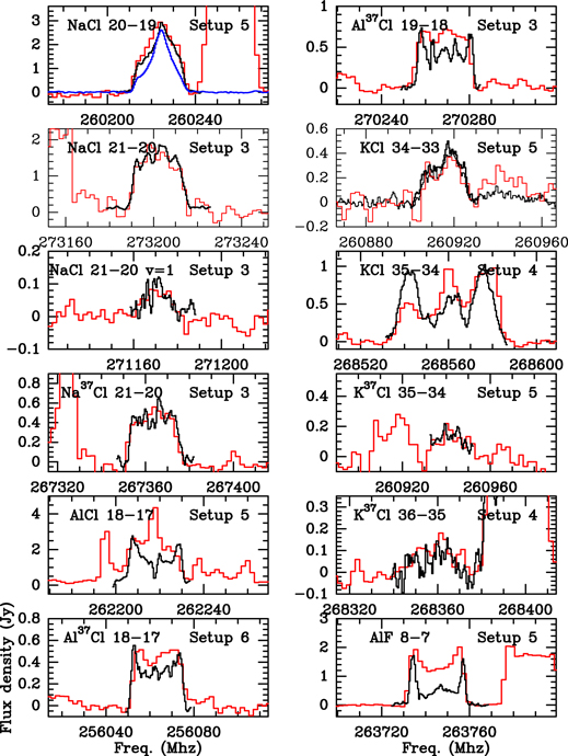
Figure 1. Comparison of the line profile obtained with the ALMA interferometer (black line) with those obtained with the 30 m single-dish radio-telescope (red line). The NaCl v = 1, J = 20–19 has not been observed at the IRAM 30 m telescope. For clarity reasons only the metal-bearing transitions are labeled in the figure. The blue line on the first panel corresponds to H13CN J = 3–2 v = (0, 11e, 0) (258936.050 MHz), shifted toward the rest frequency of H13CN J = 3–2 v = (0, 11f, 0) (260224.813 MHz). The intensity of both H13CN J = 3–2 lines is the same so the line located at 258 GHz allow us to estimate the contamination of the NaCl J = 20–19 line.
Download figure:
Standard image High-resolution imageTo conclude, Figure 1 shows that significant flux losses are only found for the channel maps of Al-bearing molecule emission. In particular, the effect is most noticeable for the most abundant isotopologues of AlF and AlCl.
3. SPATIAL DISTRIBUTION OF THE MOLECULAR EMISSION
Prior to studying the spatial distribution of the different molecules we identified possible line overlaps that could contaminate the emission from the different molecular transitions.
We found that the NaCl J = 20–19 emission line overlaps two H13CN J = 3–2 lines from vibrationally excited states, in particular the v = (0, 2, 0) (260224.828 GHz) and v = (0, 11f, 0) (260224.572 GHz) states which are closer than 2 MHz to the rest frequency of the NaCl line. A direct comparison of the NaCl J = 20–19 line with the H13CN J = 3–2 v = (0, 11e, 0) line at 258,936.05 MHz, the intensity of which is the same as that of H13CN J = 3–2 v = (0, 11f, 0), shows that the emission from the NaCl J = 20–19 transition is severely affected by the overlap (see Figure 1). In addition, NaCl J = 20–19, v = 1 might present some contamination of the H13CN J = 3–2 vibrational lines (0, 22f, 1) and (0, 22e, 1) at frequencies 258,301.911 and 258,312.299 GHz, respectively.
KCl J = 35–34 severely overlaps with intense lines from HCN in vibrationally excited states, J = 3–2 v = (0, 42f, 0) (268,545.812 GHz), and J = 3–2 v = (0, 42e, 0) (268,580.460 GHz).
Also, the AlCl J = 18–17 line overlaps with C2H  (262,208.614 GHz) and
  (262,222.585 GHz) and vibrationally excited lines of HCN, J = 3–2 v = (1, 11e, 1) and v = (1, 0, 1) (262,204.525 GHz and 262,237.296 GHz).
In the case of lines arising from vibrationally excited states, the upper level energies are high and the linewidths are narrow (Cernicharo et al. 2013), which indicates that their emission arises from the warm innermost regions of the CSE where the gas has not yet reached the terminal expansion velocity. Therefore lines from vibrationally excited states are expected to present a compact spatial distribution concentrated around the star. In this sense, in general, any extended emission could be considered to be free from line emission from highly vibrationally excited states (see Velilla Prieto et al. 2015). In the following sections we describe the molecular emission from the different species in detail.
The emission maps of the molecular transitions cited in Table 1 that are free from overlap with other lines are presented in Figures 2–4 (NaCl and isotopologues), Figures 8–10 (KCl and isotopologues), and Figures 12–14 (Al-bearing molecules). In the upper-left corner of each panel is written the vLSR of the channel, which is −26.5 km s−1 the stellar systemic velocity. As quoted above, the extended emission from AlF, AlCl, and their isotopologues is partially filtered out. However, we can still study the emission maps to understand the distribution of these molecular species in the innermost regions of IRC +10216.

Figure 2. Interferometric map of the NaCl J = 21–20 transition. The HPBW of the synthesized beam is 0704 × 0516 with a P.A. of −52 00. In the upper-left corner of each panel is written the vLSR of the channel. The lowest contour corresponds to a value of 3σ and the rest is equally spaced in jumps of 5σ with respect to the first contour. The rms of the map is σ = 3.85 mJy beam−1. The beam size is shown in the last panel. The flux density scale is in Jy beam−1.
Download figure:
Standard image High-resolution image
Figure 3. Interferometric map of the NaCl v = 1, J = 20–19 transition. This line is adjacent to other molecular transitions (Si33C2  at 258,270.23787 MHz and H13CN J = 3–2 vibrational lines (0, 22f, 1) and (0, 22e, 1) at frequencies 258,301.911 and 258,312.299 GHz, respectively. The HPBW of the synthesized beam is 0758 × 0606 with a P.A. of −594. In the upper-left corner of each panel is written the vLSR of the channel. The lowest contour corresponds to a value of 4σ and the rest are equally spaced in jumps of 2σ with respect to the first contour. The rms of the map is σ = 2.5 mJy beam−1. The beam size is shown in the last panel. The flux density scale is in Jy beam−1.
Download figure:
Standard image High-resolution image
Figure 4. Interferometric map of the Na37Cl J = 21–20 transition. The HPBW of the synthesized beam is 0709 × 0551 P.A. of 1191. In the upper-left corner of each panel is written the vLSR of the channel. The lowest contour corresponds to a value of 3σ and the rest are equally spaced in jumps of 3σ with respect to the first contour. The rms of the map is σ = 6.8 mJy beam−1. The beam size is shown in the last panel. Flux density scale is in Jy beam−1.
Download figure:
Standard image High-resolution image3.1. NaCl Emission Maps
The emission maps from the NaCl transitions are presented in Figures 2–4. As mentioned above the emission from the NaCl J = 20–19 is severely contaminated by vibrationally excited H13CN transitions. We expect this vibrationally excited emission to be restricted to the innermost regions of the molecular envelope of IRC +10216 and to be relatively narrow (Cernicharo et al. 2013). Therefore, while the emission from the inner regions might be polluted, the extended emission is most probably only a consequence of the NaCl J = 20–19 brightness distribution. In that sense, we can estimate the extent of the NaCl J = 20–19 emission. The extent of the emission in the central channels ranges between 25 and 34 in diameter, which corresponds to a radius of 2.4 1015 cm (=60 R*) and 3.3 1015 cm (=83 R*), respectively.
The molecular emission map of NaCl J = 21–20 is presented in Figure 2. The extent of NaCl J = 21–20 emission reaches a maximum radius of ∼3'' from the star in a southwest clump. The bulk of the emission is restricted to a radius of 16. A central relative minimum is clearly visible in the central maps of this transition, surrounded by two maxima. The size of this minimum is ∼05, which corresponds to a radius of 4.9 × 1014 cm (=12 R*). It is important to note that this minimum is similar to the size of the HPBW, i.e., it is spatially resolved. In addition, we can exclude this minimum to be result of a self-absorption of the NaCl emission by the cold gas closer to us, as it is visible from positive to negative velocities (vsys = −26.5 km s−1).
A detailed look at the maps reveals that the velocity field of the region where the two maxima and the minimum are located can be associated with a narrow feature in the line profile (see Figure 5). This feature is centered at the vLSR = −26.5 km s−1 and has an FWHM of ∼6 km s−1. This contrasts with the expected expansion velocity of ∼11 km s−1 (Agúndez et al. 2012) for gas lying within this region. At first glance, the structure observed is most likely explained by a torus almost edge-on, with a P.A. of ∼766. However, this P.A. is not compatible with the ∼120° P.A. of the dust lane observed by Tuthill et al. (2000) or Jeffers et al. (2014). We will show below that this disagreement in the P.A. is only apparent. A rotation of the structure responsible for the emission peaks in the central channels around the star, plus an almost face-on angle of this structure reconciles the P.A. angle observed in the ALMA interferometric maps with that observed in IR emission. In Section 3.5 we explore the brightness distributions that could result in the structures observed. Since the interferometric maps observed here observed show not only the structure but also the kinematics, the structures directly in the maps need to be carefully interpreted. In Section 4.1 we present a simple kinematic model of the structures found to be most suitable to reproduce the maps observed in Section 3.5. This allows us to constrain kinematics of the observed structures.
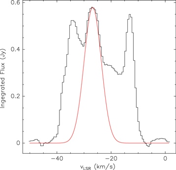
Figure 5. NaCl J = 21–20 line profile of the integrated flux density from the region that contains the two emission peaks and the central minimum (14 × 08, P.A. ∼ 766). The central component is responsible for the presence of the two maxima in the central channels of the NaCl J = 21–20 emission maps.
Download figure:
Standard image High-resolution imageThe position–velocity diagram obtained along the two maxima observed in the NaCl J = 2–1 map (Figure 6) shows that this structure is, as already mentioned, narrow in velocity, which shows that the structure responsible for these two maxima is practically static with respect to the rest of the gas. Also, the P–V diagram shows that while a maximum is slightly shifted toward positive velocities with respect to the systemic velocity, the other is shifted to negative velocities. This fact suggests that the two-peak structure is rotating. In Section 4.1 we present a simple kinematic model that supports this scenario.

Figure 6. Position–velocity diagram of the NaCl J = 21–20 emission along the two local maxima observed at central velocities (P.A. of ∼766). Flux density units are Jy beam-1.
Download figure:
Standard image High-resolution imageThe intensity of the NaCl v = 1 transitions is relatively low. Both transitions have similar intensities (see Figure 1). However, the UV coverage of the J = 20–19, v = 1 transition is much better than for the J = 21–20, v = 1 transition, which results in more reliable maps. The emission maps from the NaCl v = 1 excited state J = 20–19 are presented in Figure 3.
The extent of the NaCl v = 1 J = 20–19 transition might seem relatively large (∼1'') for a v = 1 rotational transition line. However, our observations showed that other vibrationally excited transitions such as, for instance, H13CN (0, 11f, 0) J = 3–2, which has an excitation energy of 1038.7 K, also presents an extent of ∼1''. Therefore, we could expect NaCl v = 1, J = 20–19 with an excitation energy of 649.9 K to be at least as extended as the H13CN v2 = 1 rotational transition lines.
The emission from Na37Cl J = 21–20 is remarkably similar to that of the most abundant isotopologue. The radial extent of the emission for this transition is ∼27. In particular the central relative minimum is also observed in this transition. Since the NaCl J = 21–20 and Na37Cl J = 21–20 transition map have been observed within different setups (setup 3 and setup 4, respectively) we can claim that the structures observed cannot be related to instrumental effects.
Compared with other emission maps, such as H13CN J = 3–2 or 29SiO J = 6–5 (Velilla Prieto et al. 2015; J. Cernicharo et al. 2016, in preparation), the NaCl emission is relatively compact. Despite this, several of the structures observed in Figure 2 are compatible with the spiral structure already reported by Cernicharo et al. (2015). In particular, a detailed comparison of the NaCl J = 21–20 emission with that of the two isotopomers H13CN J = 3–2 and HC15N J = 3–2 presented by J. Cernicharo et al. (2016, in preparation) showed that the spatial distribution of all these emission lines is very similar (see Figure 7). The blob observed in the NaCl J = 21–20 map at Δδ = −2 and Δα = −2 from the star is located at a spiral arm observed in H13CN J = 3–2. Also, it is important to note that the peak emission of H13CN J = 3–2 is located in the central minimum observed in the NaCl J = 21–20 map.
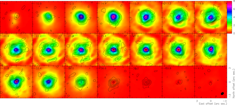
Figure 7. Contour levels of NaCl J = 21–20 from Figure 2 are overplotted to the H13CN J = 3–2 emission map from J. Cernicharo et al. (2016, in preparation). The flux density scale is in Jy beam-1.
Download figure:
Standard image High-resolution image3.2. KCl
We have obtained interferometric maps for the KCl and K37Cl J = 35–34 as well as for KCl J = 34–33 and K37Cl J = 36–35. These maps are presented in Figures 8–10, except for KCl J = 35–34 which presents severe contamination from other lines (see below).
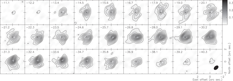
Figure 8. Interferometric map of the KCl J = 34–33 transition. The HPBW of the synthesized beam is 0866 × 0561 with a P.A. of −2286. In the upper-left corner of each panel is written the vLSR of the channel. The lowest contour corresponds to a value of 3σ and the rest are equally spaced in jumps of 2σ with respect to the first contour. The rms of the map is σ = 5.95 mJy beam−1. The beam size is shown in the last panel. The flux density scale is in Jy beam−1.
Download figure:
Standard image High-resolution image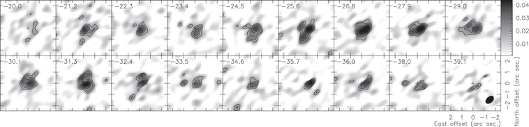
Figure 9. Interferometric map of the K37Cl J = 35–34 transition. The HPBW of the synthesized beam is 0865 × 0561 with a P.A. of −2286. In the upper-left corner of each panel is written the vLSR of the channel. The lowest contour corresponds to a value of 3σ and the rest are equally spaced in jumps of 1σ with respect to the first contour. The rms of the map is σ = 5.8 mJy beam−1. The beam size is shown in the last panel. The flux density scale is in Jy beam−1.
Download figure:
Standard image High-resolution image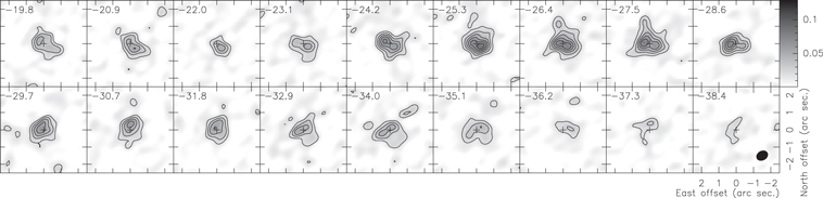
Figure 10. Interferometric map of the K37Cl J = 36–35 transition. The HPBW of the synthesized beam is 0706 × 0549 with a P.A. of −2409. This line is adjacent to the molecular transition of Si33S 15–14 (268,398.10 MHz), whose emission can be seen at the first channels of the figure. In the upper-left corner of each panel is written the vLSR of the channel. The lowest contour corresponds to a value of 3σ and the rest are equally spaced in jumps of 2σ with respect to the first contour. The rms of the map is σ = 5.8 mJy beam−1. The beam size is shown in the last panel. The flux density scale is in Jy beam−1.
Download figure:
Standard image High-resolution imageIn the case of KCl J = 34–33, the minimum in the central region of the central channels is not clearly seen due to the lower intensity of the emission, but the elongation observed seems to correspond to the two maxima observed in the central channel maps of the NaCl J = 21–20 emission. The same features can be observed in the isotopologue K37Cl J = 36–35 and J = 35–34. The extent of the KCl J = 34–33 emission is ∼25.
While KCl J = 34–33 is free from overlap with other lines, KCl J = 35–34 presents an overlap with several lines (see Section 3). However, in contrast to to the case of NaCl J = 21–20, the overlapping lines are not as close to the rest frequency of KCl J = 35–34. Therefore, as shown in Figure 11, some central channels are free of contamination from other lines. In particular, the channels between velocities −23.3 km s−1 and −25.8 km s−1 present only the emission from KCl J = 35–34. These contamination-free channels show also an elongation and a central minimum as that observed in NaCl. The KCl J = 35–34 emission map shows an extent of ∼2''.

Figure 11. KCl J = 35–34 line profile of the central pixel toward IRC +10216. A Gaussian fitting of the four transitions observed reveals that the contamination of the KCl J = 35–34 line is negligible in the range between 268,556.29–268,558.58 GHz.
Download figure:
Standard image High-resolution imageAs for NaCl, the emission from the central elongated region can be directly associated with a narrow feature in the line profile.
3.3. AlCl
As we have mentioned in Section 2.1, the extended emission from the AlCl lines is not fully recovered. In the case of AlCl J = 18–17, since it is severely contaminated by other transition lines, which are expected to come from both the innermost regions (HCN vibrationally excited) and from regions located at 15'' (C2H, see Guélin et al. 1997), we cannot determine if the emission from this AlCl transition itself is filtered out or the structure of this emission in the innermost regions.
On the contrary, the molecular lines J = 18–17 and J = 19–18 of Al37Cl present no overlap with other lines and the effect of the flux filtering is relatively small. The emission from these transitions shows a roughly spherical distribution (Figures 12 and 13).
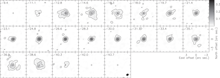
Figure 12. Interferometric map of the Al37Cl J = 18–17 transition. The HPBW of the synthesized beam is 0764 × 0611 with a P.A. of 1207. In the upper-left corner of each panel is written the vLSR of the channel. The lowest contour corresponds to a value of 3σ and the rest are equally spaced in jumps of 7σ with respect to the first contour. The rms of the map is σ = 3.73 mJy beam−1. The beam size is shown in the last panel. The flux density scale is in Jy beam−1.
Download figure:
Standard image High-resolution image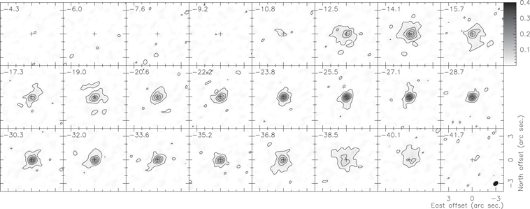
Figure 13. Interferometric map of the Al37Cl J = 19–18 transition. The HPBW of the synthesized beam is 0714 × 0515 with a P.A. of −2314. In the upper-left corner of each panel is written the vLSR of the channel. The lowest contour corresponds to a value of 3σ and the rest are equally spaced in jumps of 5σ with respect to the first contour. The rms of the map is σ = 5.56 mJy beam−1. The beam size is shown in the last panel. The flux density scale is in Jy beam−1.
Download figure:
Standard image High-resolution imageThe inspection of the innermost regions traced by the Al37Cl J = 18–17 and J = 19–18 maps reveals that the emission peaks at the continuum intensity peak. No central minimum is observed in any of the AlCl transitions.
3.4. AlF
The emission of AlF J = 8–7 is presented in Figure 14. As shown in Figure 1, this molecular transition is clearly affected by flux filtering. The central channels of this transition present only the compact emission which has not been filtered. Therefore, we cannot estimate the extent of this emission. Only at extreme velocities is the flux completely recovered. The emission at these extreme velocities is relatively extended compared with that at central velocities. This can be explained as an AlF J = 8–7 brightness distribution that peaks at the star and that is, on the large scale, diffuse and somehow homogeneous. This diffuse emission would be filtered out in the central velocity channels where it is more extended and would only be recovered in at the extreme velocities. The brightness distribution per channel observed in the AlF map is very similar to those observed in Al37Cl maps. Therefore, we might expect a similar molecular distribution for both Al-bearing molecules.

Figure 14. Interferometric map of the AlF J = 8–7 transition. The HPBW of the synthesized beam is 0858 × 0557 with a P.A. of −2286. In the upper-left corner of each panel is written the vLSR of the channel. The lowest contour corresponds to a value of 3σ and the rest of contours until 18σ are equally spaced in jumps of 3σ with respect to the first contour. From 18σ onward the intensity jump in the contours is 10σ. The rms of the map is σ = 6.4 mJy beam−1. The beam size is shown in the last panel. The flux density scale is in Jy beam−1.
Download figure:
Standard image High-resolution image3.5. Summary of the Structures Observed
After a detailed inspection of the brightness distribution of the metal-bearing transitions observed, we can separate the structures observed into two groups: the Al-bearing species shows an emission peak close to the star, while the KCl and NaCl emission maps reveal a central minimum surrounded by two peaks.
This may be interpreted at first glance as a toruslike structure rich in salts (KCl, NaCl) and poor in AlCl and AlF, while the abundance close to the star is by contrast poor in salts and rich in Al-bearing molecules.
A deep analysis of the central relative minimum shows that the two maxima located at both sides of the minimum are directly related to a particularly narrow feature (FWHM ∼ 6 km s−1) centered at the systemic velocity (Figure 5). In Section 4 we present a further analysis of the characteristics for the possible structures responsible for the observed features.
In any case, it is surprising that the toruslike structure is visible only in NaCl and KCl emission lines, while it is not seen in the Al-bearing species. It might be the case that the two maxima correspond to a larger structure, which might be suppressed due to the image deconvolution. Also, as already mentioned, recent studies have suggested the presence of a spiral structure in the ejecta around IRC +10216 (see Cernicharo et al. 2015; Velilla Prieto et al. 2015; J. Cernicharo et al. 2016, in preparation).
To explore the possibility that such a spiral is responsible for the structures observed in the NaCl and KCl maps, we have modeled a brightness distribution that consists of a Fermat spiral distribution, which is parameterized by the equation r2(θ) = a2 θ, convolved with a Gaussian function.
We used the GILDAS ALMA simulator to transform this brightness distribution into visibilities corresponding to the cycle 0 extended configuration and we generated the corresponding dirty and cleaned maps. The image restoration procedure was exactly the same as used for the ALMA on-source data. Also the integration time on-source was the same as in the observation and the UV plane coverage so obtained was similar.
In addition to this simulation, to explore other possible scenarios, we have modeled three other brightness distributions. The first brightness distribution corresponds to a toruslike structure, which for the central velocities, corresponds to two maxima plus a weak Gaussian distribution that corresponds to the rest of the emission observed in the NaCl and KCl emission maps. The brightness peak at the torus is 10 times that of the Gaussian distribution. The second distribution corresponds to a spherical shell with the size of the toruslike structure. This structure might be clumpy and appear in the maps as two maxima, similar to a torus. The third brightness distribution is a spherical shell with the addition of a Gaussian distribution.
It is important to note that the torus structure introduced for the simulations corresponds only to the central velocity channel. In this sense, for an expanding (and/or rotating) torus, the central channel will present exactly the same structure—apart from a relative rotation—except for the case in which the plane of the torus is exactly face-on. In the rest of the cases, the velocity components corresponding to the systemic velocity will appear as two maxima, varying only the P.A. of the imaginary line connecting both density peaks.
The simulations that best resemble the structures observed are those resulting from a spiral and from a Gaussian plus a torus brightness distribution (see Figures 15 and 16).
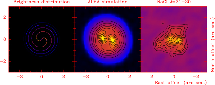
Figure 15. Left: brightness distribution of a face-on Fermat spiral with a = 0.2 at the systemic velocity. Center: result of the ALMA cycle 0 simulation of the brightness distribution for the IRC +10216 decl. For this brightness distribution no flux is filtered out. Note that this brightness distribution is restricted to the central velocity channel, which is that expected to have the largest extension and so the most affected by the flux filtering. Right: NaCl J = 21–20 emission map for the systemic velocity. The contours of the maps correspond to 10%, 20%, 30%, 40%, 50%, 60%, 70%, 80%, and 90% of the peak flux.
Download figure:
Standard image High-resolution image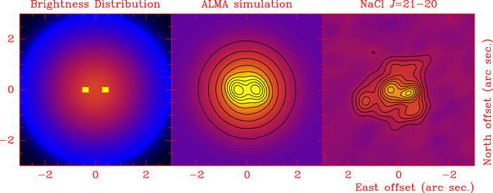
Figure 16. Left: brightness distribution of an edge-on torus plus a Gaussian distribution at the systemic velocity. The brightness peak ratio of the torus with respect to the Gaussian is 10. Center: result of the ALMA cycle 0 simulation of the brightness distribution for the IRC +10216 decl. The amount of flux recovered for the whole structure is 89%, while for the torus itself it is 100%. Note that this brightness distribution is restricted to the central velocity channel, which is that expected to have the largest extension and so the most affected by the flux filtering. Right: NaCl J = 21–20 emission map for the systemic velocity. The contours of the maps correspond to 10%, 20%, 30%, 40%, 50%, 60%, 70%, 80%, and 90% of the peak flux.
Download figure:
Standard image High-resolution imageIt has been shown that if the interferometric clean beam is remarkably elongated, i.e., if the source presents a low elevation with respect to the interferometer, a spherical shell could appear in the restored maps as two emission peaks separated by a central minimum (see HCN J = 1–0 emission map by Quintana-Lacaci et al. 2008).
A spherical shell for the decl. of IRC +10216, which results in a relatively elongated beam, could only resemble a toruslike structure if the signal to noise of the map is remarkably low. The spherical structure is visible from low fluxes to 70% of the emission peak. Therefore, the rms noise of the map should be ∼0.2 times the peak flux of the observation. In our case, this ratio is 0.022, i.e., 10 times lower, therefore any circular structure should be visible. In the case where we add a spherical Gaussian distribution, we have similar problems. While the circular structure might be less evident, we cannot reproduce the elongation observed in the ALMA KCl and NaCl maps.
It is important to understand the reasons that would prevent Al-bearing molecular transitions from presenting the two maxima observed in KCl and NaCl. The dipole moments of NaCl (9.0012 D) and KCl (10.27 D) are significantly higher than those of AlCl (1.00 D) and AlF (1.53 D). Because of this, both Al-bearing species are more easily thermalized than the salts. NaCl and KCl would be mainly thermalized in the densest regions, while AlCl and AlF emission lines would be thermalized both in dense and diffuse regions of the inner regions around IRC +10216. Therefore, we would expect to detect the emission from NaCl and KCl arising from dense regions, while Al-bearing molecules could be detected both in the arms of a spiral and in the inter-arm regions. This could be translated, in the simulations we performed, as the addition of an "inter-arm" brightness distribution in the first case of the spiral structure and in the second case as a lower brightness ratio between the torus and the Gaussian distribution.
In the case of the spiral, we add a Gaussian distribution that fills the inter-arm gaps of the spiral structure, as expected for the Al-bearing transition, with a brightness ratio between the spiral and the Gaussian of 4. The result of the simulation is that the spiral structure would disappear in the resulting map of such a brightness distribution for Al-bearing species (see Figure 17).
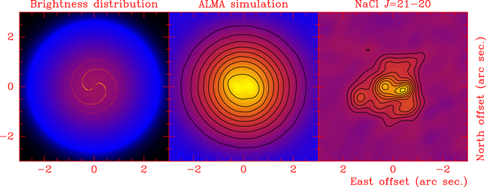
Figure 17. Left: brightness distribution of a spiral plus a Gaussian distribution. The brightness peak ratio of the spiral with respect to the Gaussian is 4. Center: result of the ALMA cycle 0 simulation of the brightness distribution for the IRC +10216 decl. The contours correspond to 10%, 20%, 30%, 40%, 50%, 60%, 70%, 80, and 90% of the peak flux. The percentage of flux recovered for the whole structure is 75%. Note that this brightness distribution is restricted to the central velocity channel, which is that expected to have the largest extent and so be the most affected by flux filtering.
Download figure:
Standard image High-resolution imageIn the case of the torus plus the Gaussian distribution, we created a brightness distribution like that of Figure 16 but with a brightness peak ratio of 2 (Figure 18). The simulation shows that also in this case, the torus would not be visible for Al-bearing species.

Figure 18. Left: brightness distribution of a torus plus a Gaussian distribution. The brightness peak ratio of the torus with respect to the Gaussian is 2. Right: result of the ALMA cycle 0 simulation of the brightness distribution for the IRC +10216 decl. The contours correspond to 10%, 20%, 30%, 40%, 50%, 60%, 70%, 80, and 90% of the peak flux. The percentage of flux recovered for the whole structure is 88%. Note that this brightness distribution is restricted to the central velocity channel, which is that expected to have the largest extent and so be the most affected by flux filtering.
Download figure:
Standard image High-resolution imageThese two simulations show that while in the Al-bearing transition maps we do not see the spiral or the torus structure, we cannot claim that these features are not present.
In summary, these simulations suggest that the most probable scenario is that the structures observed in NaCl and KCl emission maps are resulting from a spiral distribution of the molecular gas, which is in fact compatible with the spiral-like structure already observed in CO (Cernicharo et al. 2015) and recently in other species such as H13CN (J. Cernicharo et al. 2016, in preparation).
Although from NaCl and KCl it could not be possible to discard a torus structure, the lack of similar structures in HCN, SiC2, and other high dipole and abundant molecules favor the spiral structure seen in HCN.
4. NaCl EMISSION MODEL
While a detailed modeling of either a spiral or a torus structure of the circumstellar material around IRC +10216 is beyond the scope of this paper, the validity of the 1D models already available can be tested by comparing the expected results with the interferometric maps obtained, in particular for the NaCl emission.
Agúndez et al. (2012) modeled the emission from the innermost layers for a large number of transitions of several molecules (SiO, NaCl, AlF,...). This modeling relied on previous physical models of IRC +10216 and a chemical model whose initial conditions were adapted to fit the observations. We adopted a slightly modified density profile presented by Cernicharo et al. (2013) and the temperature profile presented by Agúndez et al. (2012). We used the NaCl abundance profile obtained by Agúndez et al. (2012) as starting point. The IRC +10216 model parameters are also taken from Agúndez et al. (2012) and are summarized in Table 3. The density and temperature profiles are presented in Figure 19.

Figure 19. Particle density n, gas kinetic temperature Tk, and expansion velocity vexp as a function of radius in the inner layers of IRC +10216 (Agúndez et al. 2012; Cernicharo et al. 2013).
Download figure:
Standard image High-resolution imageTable 3. IRC +10216's Model Parameters
| Parameter | Value |
|---|---|
| Distance (D) | 130 pc |
| Stellar radius (R*) | 4 × 1013 cm |
| Stellar effective temperature (T*) | 2330 K |
| Stellar luminosity (L*) | 8750 L⊙ |
| Stellar mass (M*) | 0.8 M⊙ |
| End of static atmosphere (R0) | 1.2 R* |
| Dust condensation radius (Rc) | 5 R* |
| End of dust acceleration region (Rw) | 20 R* |
| Gas expansion velocity (vexp)a | 14.5 km s−1 |
| Microturbulence velocity (Δvturb)b | 1 km s−1 |
Mass loss rate ( ) ) |
2 × 10⁻⁵M⊙ yr−1 |
| Gas kinetic temperature (Tk)c | T* × (r/R*)−0.55 |
Gas-to-dust mass ratio ( ) ) |
300 |
| Dust temperature (Td) | 800 K × (r/Rc)−0.375 |
Notes.
avexp = 5 km s−1 for regions inner to Rc, 11 km s−1 for the dust acceleration region between Rc and Rw and 14.5 km s−1 beyond Rw. bΔvturb = 5 km s−1 × (R*/r) for regions inner to Rc and 1 km s−1 in the rest of the envelope. cTk ∝ r−0.55 for regions inner to 75 R*, Tk ∝ r−0.85 between 75 and 200 R* and Tk ∝ r−1.40 beyond 200 R*.Download table as: ASCIITypeset image
Since this model assumes spherical symmetry, to be able to compare the results of the model with the observations, we have obtained the azimuthally averaged emission of the NaCl J = 21–20 and NaCl v = 1, J = 20–19 interferometric maps. In the case of a spiral, this is a reasonable first approximation.
In the case of the torus, since we need to disentangle the emission from the torus itself and from the rest of the envelope, we have obtained azimuthal cuts of the central channel of the NaCl J = 21–20 and v = 1 J = 20–19 maps along the plane of the observed toruslike structure and orthogonal to this plane. In this sense, we simulate the emission of NaCl as a sum of the spherical emission observed leaving aside the torus, plus the emission from the torus itself.
Also, we need to assume a circular beam. The size of this spherical beam is the geometric mean of the main axis of the original elliptical beam, i.e., 060 for the v = 0 J = 21–20 map and 067 for the v = 1 J = 20–19 map.
We used the radiative transfer code MADEX (Cernicharo 2012) to reproduce these two transitions of NaCl. Radiative transfer modeling requires accurate information on the molecular ro-vibrational transitions. We count on new laboratory work (C. Cabezas et al. 2016, in preparation) which has allowed us to include in our radiative transfer code vibrational transitions up to Δv = 8 with new derived dipole moment values for the ro-vibrational transitions up to v = 8. In addition, we present the first estimates of the collisional rates of NaCl with He for v ≤ 8 and Δv ≤ 4 in the
4.0.1. Model Fitting
For our model we considered up to J = 100 and v = 5. We divided the spherical envelope into 100 concentric shells and solved the excitation conditions of NaCl in each shell assuming a large velocity gradient approximation, which assumes that each shell of the envelope is radiatively isolated. Therefore, we can solve the statistical equilibrium equation in each shell.
For both the spiral and the torus scenarios we have only varied the NaCl abundance profile, while we have kept unaltered the H2 density profile presented by Cernicharo et al. (2013).
In the case of the spiral structure, the best fit for the azimuthally averaged emission of NaCl J = 21–20 and v = 1, J = 20–19 maps is presented in Figure 20. The abundance profile obtained is presented in Figure 21. This abundance profile is that presented by Agúndez et al. (2012), multiplied by 1.2, except for two regions, one located between 1015 cm and 2.6 × 1015 cm which has to be multiplied by 1.5 and a region with negligible abundance of NaCl located between 2.5 × 1015 cm and 3.4 × 1015 cm. The intermediate empty region is most probably related to the spiral structure itself and traces the inter-arm region.

Figure 20. Best fit for the azimuthally averaged brightness distribution of NaCl v = 0, J = 21–20 (black line) and of the v = 1, J = 20–19 (red line) for the central velocity channel within the spiral scenario. The model is plotted in solid lines and the observations in dashed lines.
Download figure:
Standard image High-resolution image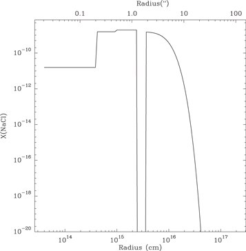
Figure 21. Abundance profile obtained for the spiral scenario.
Download figure:
Standard image High-resolution imageWe estimate the mass of the spiral to be 1.6 × 1032 gr (=0.08  ) and the NaCl mass in the spiral to be 1.0 × 10²² gr (=1.7 × 10⁻⁶MEarth).
In addition, we have used the averaged density to fit the single-dish emission profiles from the NaCl transitions J = 7–6 to J = 27–26 presented by Agúndez et al. (2012; Figure 22). Most of these lines are relatively well fitted, showing that the model obtained from the NaCl J = 21–20 ALMA interferometric maps also is able to reproduce the single-dish NaCl line profiles from low-energy to high-energy transitions. The NaCl J = 20–19 line shows a poor fit, but this is a result of the aforementioned blending of this line with the H13CN J = 3–2 v = (0, 11f, 0) transition.
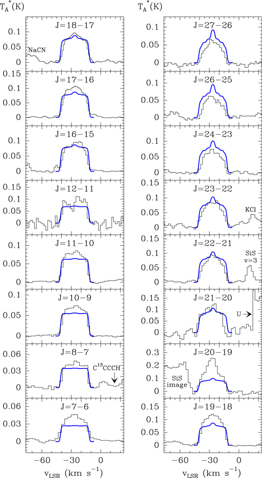
Figure 22. Line fitting result for the NaCl profiles presented by Agúndez et al. (2012) obtained for the spiral model.
Download figure:
Standard image High-resolution imageIn the case of the torus, the fitting of the two cuts is presented in Figure 23. We have found that the torus should have a minimum and maximum radius of 4 × 1014 cm and 1.1 × 1015 cm, respectively, which corresponds to ∼27 AU and ∼73 AU. We found the fractional abundance of NaCl in the torus to follow an r3 law (Figure 24).
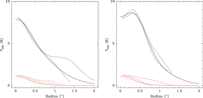
Figure 23. Best fit of the model for the azimuthal cuts along the plane of the torus (right) and orthogonal to it (left) for the central velocity, for the NaCl J = 21–20 (black lines) and NaCl v = 1 J = 20–19 (red lines) transitions. The model is plotted in solid lines and the observations in dashed lines. The two dotted lines for each cut represent the positive and negative offsets with respect to the center of the map.
Download figure:
Standard image High-resolution image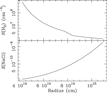
Figure 24. Density profile and NaCl abundance profile obtained to fit the torus emission of the azimuthal cut along its plane.
Download figure:
Standard image High-resolution imageThe azimuthally averaged emission has been fitted using an average of the two density profiles obtained, i.e., that of the torus and of the spherical emission. We have found an appropriate fit for the azimuthally average emission assuming that 65% of the emitting mass comes from the torus-free abundance profile and 35% from the torus NaCl abundance profile. The result of azimuthally averaging a torus would result in a spherical hollow shell. Therefore, as this scenario consists of a spherical shell plus a torus, the azimuth average of these two structures can be regarded as a spherical torus-free shell plus a hollow shell, a result of the torus. In that sense, we can estimate the mass of this simulated spherical shell as:

where  . Therefore, we can estimate the total mass of the torus as:

The mass of the torus obtained is 2.1 × 1029 gr (=1.1 × 10⁻⁴ ), and the total mass of NaCl in the torus is 8.7 × 10¹⁹ gr (=1.5 × 10⁻⁸ MEarth).
In both cases, we found significant departures in the quality of the fits for mass variations larger than 20%.
4.1. Kinematic Model
In order to understand the kinematic characteristics of the structures, the spiral or the torus, observed in the NaCl and KCl emission maps, we have developed a simple model of expanding and rotating spiral and torus structures. The aim of this model is to understand the kinematics and spatial distribution expected for different structures.
We adopted as the P.A. of the spiral and the torus that of the dust lane observed by Jeffers et al. (2014) and Tuthill et al. (2000) (P.A. = 120°). In order to generate a kinematic model that qualitatively reproduces the observations we have to find the value of three parameters: the expansion velocity (vexp), the rotation velocity (vrot), and the inclination with respect to the plane of the sky (i). For a fixed parameter, any of the three aforementioned, the other two are intercorrelated, i.e., for a fixed inclination, only one combination of vrot and vexp fits the observations. The expansion velocity at the regions where we have found the inner radius to lie is relatively well constrained to be between ∼11 km s−1 (Fonfría et al. 2008) and ∼12.5 km s−1 (Decin et al. 2010). The difference in the inclination and the rotation velocity is negligible when assuming the former or the latter expansion velocity.
We do not have any information on the possible tilt of the orbital plane of the spiral or the torus with respect to the plane of the sky. CO maps from Cernicharo et al. (2015) suggest that the inclination of the spiral is close to face-on. In any case, the inclination with respect to the plane of the sky together with the rotation has a direct effect on the P.A. of the structures observed in the maps. In particular, except for the edge-on case, a rotation in the spiral/torus would result in a P.A. rotation of the plane of the spiral/torus in the observed velocity maps.
We simulated the density maps at each velocity for a Fermat spiral or for a torus with a radial density profile and inner and outer radius such as those obtained in the previous section. These density maps were convolved with the beam of the NaCl J = 21–20 line and compared with these emission maps in order to obtain the best possible fit to the observations.
Since we expect our estimate of the expansion velocity of the spiral/torus and the P.A. of the dark lane observed in IR emission is well constrained, we could use our kinematic model to constrain the inclination of the orbital plane with respect to the plane of the sky. We compared the kinematic model with the observations varying the inclination angle between 90° and 0°. We found the best fit for i ∼ 15 ± 10°.
Note that since we present density maps, we do not take into account any excitation effects or possible self-absorptions. The aim of the model is to understand the kinematics of the spiral and of the torus, but not to completely reproduce the observations.
The parameters for which we found the best fit are presented in Table 4. The comparison between the models (contours) and the NaCl J = 21–20 emission map (colors) is presented in Figure 25. The rotation of the spiral/torus is in fact the reason why the NaCl maps present an elongation with a P.A. of ∼766 while the real P.A. of this feature is coincident with the dust lane observed by Tuthill et al. (2000), i.e., ∼120°.

Figure 25. Top: simulation of an expanding and rotating spiral overplotted on the NaCl J = 21–20 emission map. Bottom: simulation of an expanding and rotating torus overplotted on the NaCl J = 21–20 emission map. In both cases the ALMA data were Hanning smoothed to 0.49 MHz, while the effective spectral resolution is 0.98 MHz. We present these channels as this allows seeing the changes in the kinematic model more accurately.
Download figure:
Standard image High-resolution image
Table 4. IRC +10216's Spiral/Torus Kinematic Model Parameters
| Parameter | Value |
|---|---|
| Rin | 02 |
| Routa | 056 |
| i | 15° |
| P.A. | 120° |
| Vexp | 11 km s−1 |
| Vrot | 8 km s−1 |
Note.
aOuter radius for the torus case.Download table as: ASCIITypeset image
As we have mentioned, this model is a just first approximation. In order to accurately derive the properties of the innermost structures observed a 2D radiative transfer code is essential.
5. RESULTS
We have detected the presence of a slowly expanding structure around IRC +10216 in the emission from the NaCl and KCl salts. Our simulations and the presence of a spiral observed in CO and other species (Cernicharo et al. 2015; J. Cernicharo et al. 2016, in preparation, e.g.), suggest that this structure most probably corresponds to a spiral distribution of material around IRC +10216. However, the presence of a circumstellar torus could also reproduce the observed structures. We also found that the gas seems to be rotating around the star. In addition, the model presented in Section 4 revealed that the abundance of NaCl at radii lower than ∼10 R* is significantly low compared with that of outer regions.
The presence of this central minimum observed in NaCl and KCl emission maps could be intrinsic to these salts (chemical origin) or could be related to the spatial distribution of matter at these small scales (physical origin).
The lack of NaCl and KCl in the innermost regions is expected to be related to chemical processes. Agúndez et al. (2012) showed that, in order to fit the observations, LTE calculations in the regions inner to 10 R* require an abundance that is remarkably lower than that needed in the outer regions to fit the interferometric and single-dish data. Therefore, no density hole in the gas ejected is needed to reconcile the minimum observed and the models.
The inner structure detected in NaCl and KCl is very similar to the dust lane observed by Jeffers et al. (2014). In particular, the inner and outer radii are similar to the ring model presented by these authors. However, we find a difference of the P.A. of both elongations. Assuming a rotation of the spiral/torus we found that in order to reconcile both P.A. angles the orbital plane should be tilted by ∼15 ± 10° with respect to the plane of the sky.
As we have seen, the spiral/torus would remain undetectable if the ratio between the brightness distribution of the arm/inter-arm regions in the first case, or the ratio between the spherical shells and the torus in the second scenario is low enough. This might be the case for the Al-bearing molecules since the AlF and AlCl emission would trace both dense and diffuse zones, which correspond to the arm and inter-arm regions, respectively. In contrast, NaCl and KCl emission would arise mostly from dense regions formed by the spiral arms.
The interferometric maps of the Al-bearing transitions suggest that the emission from these molecules is relatively extended (≳25), as seen at the extreme velocities, but also present a significant intensity increase in the innermost regions. Since part of the most extended emission has been filtered out, we cannot determine the real extent of the emission from these molecules.
5.1. Origin of the Observed Circumstellar Structures
As we have shown, the inner structures observed in the NaCl and KCl maps might correspond to the innermost regions of the spiral observed in CO by Cernicharo et al. (2015).
Jeffers et al. (2014) suggested that the origin of the dust lane observed is the interaction with a binary. These authors also suggested that the orbital plane of the binary is nearly edge-on. However, Cernicharo et al. (2015) and J. Cernicharo et al. (2016, in preparation) presented models that showed that the spiral structure observed in CO can only be a consequence of an interaction with a binary with the orbital plane close to face-on and having episodic mass-loss ejections. Our kinematic model also suggests that the orbital plane of the spiral is close to face-on. In particular, the structure observed might just be the inner regions of the spiral structure observed in CO by Cernicharo et al. (2015).
In case the structure responsible for the features observed is a spiral, its origin would be the partner star itself. The NaCl mass derived assuming this scenario is 1.0 × 10²² gr (=1.7 × 10⁻⁶ MEarth), which is ∼0.2 times the mass of NaCl found in the Earth's oceans.
The absence of the features in the Al-bearing interferometric maps might be related to the different dipole moment of the salts and the Al-bearing species observed. This would result in the NaCl and KCl brightness distributions being much more sensitive to density than those of AlCl and AlF. Our simulations have shown that the presence of diffuse emission would prevent the detection of the two maxima from being observed in the Al-bearing molecules.
5.2. Structures around IRC +10216. A Proposed Global Scenario
IRC +10216 has been extensively imaged at different wavelengths and with very different spatial resolutions. All of these observations can be combined to build a complete view of the circumstellar environment of IRC+10216 IRC +10216.
We can divide the structures observed in IRC +10216 mainly into four different groups: the spiral/concentric shells, an outflow, a dark lane and a large-scale bow shock recently observed by Sahai & Chronopoulos (2010) in UV emission. This bow shock was found at 21' and was suggested to be the result of the interaction of the IRC +10216 molecular gas with the ISM. This has been later confirmed by Matthews et al. (2015), who have detected a H i shell coincident with the UV emission observed by Sahai & Chronopoulos (2010). This H i emission presents both a density enhancement at the edge of the H i shell and a slight velocity decrease with respect to the inner molecular gas. These two effects are explained by the interaction of the H i shell with the ISM.
The concentric shells were first observed in dust scattered light (Mauron & Huggins 2000). They found irregularly spaced shells reaching a radius of ∼50''. These shells also have been observed in CO emission extending up to ∼180'' from the star (see, e.g., Fong et al. 2003; Cernicharo et al. 2015). Both Mauron & Huggins (2000) and Cernicharo et al. (2015) argued that the formation of these shells was compatible with a spiral structure which suggested the presence of a binary system. Our analysis of the kinematics of the inner structure suggest that the orbital plane is tilted with respect to the plane of the sky by 15 ± 10°.
In the sub-arcsecond scale, an elongation with a P.A. of ∼20° has been observed at 2 μm (Weigelt et al. 1998) with an extent of ∼300 mas, also in the V-band by Mauron & Huggins (2000), and in molecular emission by, e.g., Fonfría et al. (2014) and Velilla Prieto et al. (2015). This elongation has been suggested to be related to a bipolar outflow (Fonfría et al. 2014; Tuthill et al. 2000).
Also, the 2 μm observations obtained by Weigelt et al. (1998) revealed a dark lane almost orthogonal to the bipolarity observed. This dark lane was also inferred by Tuthill et al. (2000) and later on confirmed by Jeffers et al. (2014), who obtained polarized light images of IRC +10216. In addition, we have found that this dust lane is compatible with the presence of a rotating spiral or torus.
All these observations suggest that IRC +10216 has been ejecting mass episodically, and the resulting ejecta have been clearly influenced by the presence of a partner star orbiting in a plane close to the plane of the sky. In the innermost regions, observations suggest the presence of a NaCl-rich structure, rotating in the same plane as the orbital plane of the binary system. Orthogonal to this plane, there is an outflow observed in molecular emission and visible light. This structure observed in NaCl might be the inner regions of the spiral observed at larger scales, which is visible in NaCl and KCl emission thanks to the high dipole moment compared with AlF and AlCl.
6. CONCLUSIONS
We present high spatial resolution interferometric maps obtained with ALMA for metal-bearing transitions toward IRC +10216. These maps reveal that the emission of these transitions is particularly compact compared with other molecules such as CO, H13CN or SiS.
In these maps, we have identified an elongation in the NaCl and KCl distributions. This elongation has been found to be probably a spiral or a torus orbiting around the star. This structure is not observed in the Al-bearing transitions, probably due to the difference in the dipole moments of these two sets of molecules.
We modeled the data assuming both the most probable spiral case and a scenario where the observed features could arise from the presence of a torus.
For the spiral structure, we find an inner minimum similar to that of the torus scenario, i.e., ∼27 AU in radius. In this case, all NaCl emission is assumed to arise from a single structure. The NaCl mass obtained in this case is 1.0 × 10²² gr.
For the torus scenario, the inner and outer radii of the torus obtained are ∼27 AU and ∼73 AU, respectively. The total mass estimated for the torus is 2.1 × 1029 gr and the NaCl mass derived for the torus is 8.7 × 10¹⁹ gr.
Assuming the expansion velocity to be 11 km s−1 as suggested by previous works, we found that the structure is rotating at ∼8 km s−1 and slightly tilted with respect to the plane of the sky (i ∼ 15 ± 10°).
Future maps with high angular and spectral resolution would allow us to better constrain the characteristics of the structures detected here. In addition, these high angular and spectral resolution maps would allow us to study with high accuracy the velocity field of the innermost regions. Furthermore, a smaller beam would allow us to detect the presence of these inner structures in other metal-bearing and C-rich molecules.
The research leading to these results has received funding from the European Research Council under the European Union's Seventh Framework Programme (FP/2007-2013)/ERC Grant Agreement n. 610256 (NANOCOSMOS). We would also like to thank the Spanish MINECO for funding support from grants CSD2009-00038, AYA2009-07304 and AYA2012-32032. Y.K. acknowledges the use of HPC resources of SKIF-Cyberia (Tomsk State University). We thank Marcelo Castellanos for useful discussions.
APPENDIX: NaCl RATE COEFFICIENTS
In this Appendix, we briefly describe the computation of inelastic rate coefficients for the ro-vibrational excitation of NaCl by He that were used to model NaCl emission. Within the Born–Oppenheimer approximation, the study of inelastic collisions requires two steps: (i) the calculation of an ab initio potential energy surface (PES) between the particles in collision and (ii) the study of the dynamics of nuclei on this surface.
A.1. NaCl PES
In the present work, the Jacobi coordinate system was used. The center of the coordinates is placed in the NaCl center of mass (c.m.), and the vector R connects the NaCl c.m. with the He atom. The rotation of the NaCl molecule is defined by the θ angle. The calculations were performed for eight NaCl bond lengths r = [4.0, 4.2, 4.35, 4.46125, 4.65, 4.85, 5.0, 5.1] a0, where a0 is the Bohr radius, which allows us to take into account vibrational motion of NaCl molecule up to v = 4.
The intermolecular coordinates θ and R were varied from 0° to 180° by step of 10° and from 2.75 to 40 a0 accordingly. In order to better represent the repulsive part of the PES, we have interpolated the ab initio calculations on a fine grid of θ angles for each r distance in order to use more angles in the fitting procedure.
All electronic-structure calculations were performed using the MOLPRO program (Werner et al. 2010). The ab initio calculations were carried out using the coupled cluster approach with perturbative treatment of triple excitations (CCSD(T)) (Hampel et al. 1992) with a correlation-consistent weighted core-valence quadruple zeta (aug-cc-pwCVQZ) basis set (Prascher et al. 2011) which accounts for the core–core and core–electron correlation effects. Bond functions were placed midway between the He atom and the NaCl c.m. to permit a better description of correlation effects. In the calculations of the interaction energies, the basis set superposition error was corrected using the counterpoise scheme (Boys & Bernardi 1970).
The PES V(R, θ, r) was fitted to the analytical form:
where re was taken to be 4.46125 a0. Bl,n(R) are the expansion coefficients and their radial dependence is represented as cubic splines. The basis functions Pl0(cos(θ)) are the Legendre polynomials. In our fit, N = 8 and M = 20.
A.2. Scattering Calculations
A.2.1. Rotational Excitation of NaCl by He
The three-dimensional (3D) PES was then used for quantum scattering calculations. In the calculations, we neglect the hyperfine splitting of the NaCl rotational levels (j) due to Na and Cl non zero nuclear spins. Hyperfine resolved rate coefficients can be obtained from the present data using recouping techniques as described in Faure & Lique (2012).
First, we performed pure rotational excitation calculations using the 3D PES with the NaCl bond length fixed at ground state vibrationally averaged value (r0 = 4.4696 a0, Caris et al. 2002). Because the exact close-coupling (CC) approach of Arthurs & Dalgarno (1960) is very computationally intensive for molecules with small rotational constants, we used the coupled-states approximation (CS) (McGuire & Kouri 1974) for the determination of cross sections between rotational levels ![$[\sigma (j\to {j}^{\prime })].$](https://content.cld.iop.org/journals/0004-637X/818/2/192/revision1/apj522531ieqn12.gif)
The validity of the CS approach compared to a full CC approach has been tested for selected energies. It is found that the CS approach can lead to inaccuracies of 20–30% for low-energy cross sections (<50 cm−1), but agreement improves between CC and CS cross sections when the energy is greater than 50 cm−1, and we expect that the CS rate coefficients will be accurate as soon as we considered temperatures above 20–30 K.
The standard time-independent coupled scattering equations were solved using the MOLSCAT code (Hutson & Green 1994). The calculations were carried out using the propagator of Manolopoulos (1986) with integration range from 2.75 to 40 a0. The reduced mass of the complex was set to μ = 3.764 a.m.u. In order to converge the inelastic cross sections between the first 81 rotational levels of NaCl, the rotational basis set was extended, at high collisional energy, up to j = 100. The rotational spectroscopic constants were taken from Caris et al. (2002).
Using the above methodology, we obtained the energy variation of the excitation cross sections between the first 81 rotational states of NaCl. Rotationally resolved coefficients were obtained by averaging the appropriate cross sections over a Boltzmann distribution of velocities at a given kinetic temperature T:

where  and kB is the Boltzmann constant. The total energy E is related to the kinetic energy according to
  where
where  j is the energy of the initial rotational level. The calculations were carried out up to total energy (E) of 10000 cm−1 which allowed us to get, after averaging, the rate coefficients for temperatures ranging from 5 to 1500 K.
A.2.2. Ro-vibrational Excitation of NaCl by He
Then, we have performed ro-vibrational excitation calculations using the 3D PES. The Vibrational Close-Coupling rotational Infinite Order Sudden (VCC-IOS) method (Parker & Pack 1978) was employed to obtain the inelastic cross sections for the ro-vibrational excitation of NaCl by He.
In the VCC-IOS approximation the matrix elements of the potential between vibrational states of the NaCl molecule are required for each R and θ are expressed as:

The NaCl vibrational wave functions  were obtained by the DVR method of Colbert & Miller (1992) from a NaCl potential calculated at the same level of accuracy as the NaCl–He PES (without the inclusion of midbond functions). The vibrational wave functions were taken with j = 0.
Within the VCC-IOS approach, the rotational levels are treated as being degenerate. Hence, the problem reduces to the computation of vibrationally (in)elastic S-matrix elements calculated with a close-coupling approach at fixed values of the θ Jacobi angles for a given L-value (L is a relative angular momentum quantum number). This fixed-angle S-matrix elements must then be multiplied by the appropriate spherical harmonics and integrated over θ to give the fundamental IOS cross sections  (E) out of the v, j = 0 level.
The de-excitation ro-vibrational cross sections are expressed in a reduced form in terms of the  cross sections of Parker & Pack (1978):
where the large parentheses denote the "3-j" symbols; v, j and v', j' are, respectively, the initial and final vibrational and rotational states.
The time-independent scattering equations were solved using the MOLSCAT code of Hutson & Green (1994) in order to obtain the fundamental  cross sections. Similar parameters to those used in the calculations for the pure rotational excitation were used. In order to converge the cross sections for v = 0–3, the v = 4 vibrational level was also included. The summation in Equation (6) was performed for L from 0–201. The vibrational spectroscopic constants were taken from Brumer & Karplus (1973).
Using the above methodology, we obtained the energy variation of the (de-)excitation cross sections ( ) between the ro-vibrational states of NaCl with v ≤ 3 and j ≤ 80. Corresponding rate coefficients were obtained by averaging the appropriate cross sections over a Boltzmann distribution as for the pure rotational excitation. Cross section calculations up to a total energy (E) of 10,000 cm−1 allowed us to get after averaging the rate coefficients for temperatures ranging from 100 to 1500 K.
As NaCl is a heavy molecule with a small rotational constant, the IOS approach, although it neglects the energy structure of the rotational levels and is expected to be poor at low energies, seems to be appropriate for the temperature range considered in this work. The fact that the CS and the VCC-IOS rate coefficients agree well for the v = 0 state confirms the hypothesis.
Footnotes
- 10
This paper makes use of the following ALMA data: ADS/JAO.ALMA#2011.0.00229.S. ALMA is a partnership of ESO (representing its member states), NSF (USA), and NINS (Japan), together with NRC (Canada) and NSC and ASIAA (Taiwan), in cooperation with the Republic of Chile. The Joint ALMA Observatory is operated by ESO, AUI/NRAO, and NAOJ.
- 11
- 12
- 13
A specific Fortran code to calculate the collisional rates for a selected ro-vibrational transition and a certain gas temperature is included in this paper. It can also be downloaded at https://zenodo.org/record/42262 (Quintana-Lacaci et al. 2015).