


ABSTRACT
Coronal rain composed of cool plasma condensations falling from coronal heights along magnetic field lines is a phenomenon occurring mainly in active region coronal loops. Recent high-resolution observations have shown that coronal rain is much more common than previously thought, suggesting its important role in the chromosphere-corona mass cycle. We present the analysis of MHD oscillations and kinematics of the coronal rain observed in chromospheric and transition region lines by the Interface Region Imaging Spectrograph (IRIS), the Hinode Solar Optical Telescope (SOT), and the Solar Dynamics Observatory (SDO) Atmospheric Imaging Assembly (AIA). Two different regimes of transverse oscillations traced by the rain are detected: small-scale persistent oscillations driven by a continuously operating process and localized large-scale oscillations excited by a transient mechanism. The plasma condensations are found to move with speeds ranging from few km s−1 up to 180 km s−1 and with accelerations largely below the free-fall rate, likely explained by pressure effects and the ponderomotive force resulting from the loop oscillations. The observed evolution of the emission in individual SDO/AIA bandpasses is found to exhibit clear signatures of a gradual cooling of the plasma at the loop top. We determine the temperature evolution of the coronal loop plasma using regularized inversion to recover the differential emission measure (DEM) and by forward modeling the emission intensities in the SDO/AIA bandpasses using a two-component synthetic DEM model. The inferred evolution of the temperature and density of the plasma near the apex is consistent with the limit cycle model and suggests the loop is going through a sequence of periodically repeating heating-condensation cycles.
Export citation and abstract BibTeX RIS
1. INTRODUCTION
High-resolution observations from recent solar missions have unveiled a dynamic nature of the solar corona and enabled us to study the coronal activity in unprecedented detail (Scullion et al. 2014). The basic structure of the corona is formed by coronal loops, magnetic flux tubes confining the coronal plasma threading through the solar surface. They are highly dynamic and are subject to a range of matter and energy transport processes. One of such processes is coronal rain, consisting of cool plasma condensations falling from coronal heights to the solar surface guided by magnetic field lines (Schrijver 2001; De Groof et al. 2004).
Although first observed more than 40 years ago (Kawaguchi 1970; Leroy 1972), coronal rain has not received much attention until recent years. This was partially due to the lack of instruments with resolution sufficient for detailed observations. Coronal rain was also believed to be a relatively rare phenomenon occurring only sporadically in active regions on the timescales of days (Schrijver 2001). Recent work has, however, shown that the coronal rain is, in fact, much more common than previously thought, typically occurring on timescales of hours (Antolin et al. 2010; Antolin & Rouppe van der Voort 2012). This short period of a typical heating-condensation cycle, together with the fact that a significant fraction of coronal loops are out of hydrostatic equilibrium constantly undergoing heating and cooling phases (Aschwanden et al. 2001), making it likely that condensation will occur, suggest that coronal rain may have an important role in the chromosphere-corona mass cycle (Marsch et al. 2008; Berger et al. 2011; McIntosh et al. 2012).
The formation of coronal rain is believed to be linked to rapid cooling of thermally unstable coronal loops (Müller et al. 2003, 2004, 2005). Concentrated footpoint heating leads to an uneven temperature profile along the loop length. Chromospheric evaporation and direct injection of plasma into the corona result in high densities near the top of the loop. In the case of insufficient thermal conduction, the radiation losses near the loop top overcome the heating input, resulting in the onset of a thermally unstable regime. A perturbation to the loop such as a shock wave can then trigger catastrophic cooling, leading to the formation of condensations which subsequently fall down toward the solar surface along the magnetic field lines within the coronal loop. This process continues until the heating and cooling regain equilibrium and pressure balance is restored.
The cooling sequence of the loops predicted by the instability model has been investigated by a number of multi-channel observations. The EUV intensity variations of the active region loops has been analyzed using TRACE observations with loop tops brightening first in 195 Å and then in 171 Å channel (Schrijver 2001), and by combining observations from the Solar and Heliospheric Observatory (SOHO) Extreme Ultraviolet Imaging Telescope (EIT) and the Big Bear Solar Observatory with coronal rain plasma first showing in 304 Å channel followed by Hα (De Groof et al. 2005). Sequential brightening and subsequent fading of multiple loop structures has also been observed in soft X-ray and EUV channels using TRACE and Soft X-Ray Telescope (SXT; Ugarte-Urra et al. 2006) and Hinode EUV Imaging Spectrometer (EIS; Ugarte-Urra et al. 2009), both pointing toward continuous heating and cooling scenarios. The cooling sequence has also been observed in loops exhibiting coronal rain (Antolin et al. 2015b). Such peak intensity variations with time and wavelength are therefore likely to be a signature of the thermal instability in the loops. On larger scales, the occurrence interval of the thermal instability onset leading to the formation of the coronal rain in a loop with footpoint-concentrated heating is estimated to be on a timescale of several hours (Antolin & Rouppe van der Voort 2012). Similar long-term periodic EUV pulsations with periods of several hours were observed in warm active region coronal loops (Auchère et al. 2014; Froment et al. 2015), as well as in prominences (Foullon et al. 2004, 2009).
Coronal rain is usually observed in emission in cool chromospheric lines of both neutral (Hα, Lyα) and ionized atoms (Ca ii, He ii), or in absorption in EUV (Schrijver 2001). The temperatures of the rain plasma range from the transition region ( K) to chromospheric (
 K). Coronal rain has been detected in the 304 Å channel of the Solar Dynamics Observatory (SDO) Atmospheric Imaging Assembly (AIA; Kamio et al. 2011) and SOHO/EIT (De Groof et al. 2004, 2005), in the 1600 Å channel of TRACE (Schrijver 2001), in Ca ii H line using Hinode Solar Optical Telescope (SOT; Antolin et al. 2010; Antolin & Verwichte 2011), in the Hα by the Swedish Solar Telescope (SST)/CRISP (Antolin & Rouppe van der Voort 2012), and in IRIS FUV and NUV channels (Kleint et al. 2014). Material resembling coronal rain has recently been observed in photospheric wavelengths by SDO Helioseismic and Magnetic Imager (HMI; Martínez Oliveros et al. 2014). Although the best resolved coronal rain is usually observed off-limb, some on-disk coronal rain events have also been observed (e.g., Antolin et al. 2012; Antolin & Rouppe van der Voort 2012).
The thermal instability onset and the process of the formation and evolution of coronal rain have been subject to a number of numerical studies. Such studies were initially restricted to simplified one-dimensional (1D) cases. One of the first attempts to model the formation of the condensation region and its subsequent evolution was done by Müller et al. (2003, 2004, 2005), indicating that a loop with exponential heating function localized at the footpoints develops a thermal instability followed by catastrophic cooling. This basic model was further expanded by Antolin et al. (2010) by accounting for variable loop cross-sections, the impulsive nature of heating, and Alfvén wave dissipation near footpoints. More recently, the formation process of coronal rain condensations and their evolution was studied by 2.5D MHD simulations (Fang et al. 2013, 2015). The evolution of condensations for the case of fully ionized plasma was further analyzed by Oliver et al. (2014), emphasizing the role of the pressure effects on the coronal rain dynamics.
The small size of coronal rain blobs makes them suitable for tracing the strength and structure of the coronal magnetic field (Antolin & Rouppe van der Voort 2012). The degree to which the rain follows the direction of the magnetic field, however, depends on the strength of the coupling between recombined atoms created during the condensation phase and the local ion population. In the case of the strong coupling, any disturbance of the magnetic field in the loop will be reflected in the motion of the rain blobs. A number of observations have shown the presence of transverse MHD waves in the coronal loops (Aschwanden et al. 1999; Nakariakov et al. 1999). These are commonly interpreted as a fast kink MHD mode (Edwin & Roberts 1983; Nakariakov & Verwichte 2005; Van Doorsselaere et al. 2008; Goossens et al. 2009). Multiple regimes of such oscillations have been detected, ranging from periods on the order of seconds (e.g., Williams et al. 2001) to hours (e.g., Hershaw et al. 2011). Both standing (Nakariakov et al. 1999; White & Verwichte 2012) and traveling regimes (Williams et al. 2001; Tomczyk et al. 2007; McIntosh et al. 2011) of the kink oscillations are observed. They can be excited by a flare or another energetic event and subject to rapid attenuation (White et al. 2012; White & Verwichte 2012; Nisticò et al. 2013), possibly caused by resonant absorption (Hollweg & Yang 1988; Goossens et al. 2002, 2010; Ruderman & Roberts 2002; Antolin et al. 2015a; Okamoto et al. 2015), or persistent and decayless, driven by a continuous process (Wang et al. 2012; Anfinogentov et al. 2013; Nisticò et al. 2013). Coronal rain occurring in a loop oscillating transversely will also be subject to transverse oscillatory motion. Such MHD oscillations in coronal rain were first detected by Antolin & Verwichte (2011). In the case of a non-negligible inertia of the coronal rain blobs, the rain itself can have an effect on the loop oscillations.
MHD oscillations in coronal rain can therefore (1) affect dynamics of the coronal rain through a ponderomotive force (PMF) exerted on the falling blobs, (2) help to quantify the effect of the plasma condensations on the coronal loop and (3) have coronal seismological potential and be a source of information about coronal loop properties and the magnetic field structure in the loop. This highlights the importance of addressing the interplay between the coronal rain and MHD waves in order to better understand the coronal loop structure, evolution and energy transport mechanisms.
The paper is organized as follows: Section 2 covers the details of IRIS, Hinode/SOT, and SDO/AIA observations used for analysis and the methods used for data processing. Section 3 focuses on analysis of MHD oscillations detected in the coronal rain. In Section 4 we investigate the kinematics of individual coronal rain blobs and present statistics of blob velocities and accelerations. In Section 5 we analyze the evidence for the thermal evolution of the loop plasma and the heating-condensation cycle of the coronal loop responsible for the coronal rain formation. Section 6 contains detailed discussion of the analysis outcomes and their implications. The work is summarized in Section 7.
2. OBSERVATION AND DATA PROCESSING
We focus on observations taken by IRIS (De Pontieu et al. 2014), AIA on board SDO (Lemen et al. 2012), and SOT on board Hinode (Tsuneta et al. 2008). The data set analyzed below was taken as a part of Hinode–IRIS–SST coordination (HOP 262) during a 2014 August observing campaign. An event from 2014 August 25 near NOAA AR 12151 is analyzed using coordinated IRIS–Hinode observations and complemented by full-disk SDO/AIA data. We used IRIS level 2 SJI data taken between 7:46 and 10:30 UT retrieved from mission web page (http://iris.lmsal.com/search) in the NUV (Mg ii k) and FUV (Si iv) filters with an exposure time of 8 s, 19 s cadence, and the field of view centered at ![$[-984^{\prime\prime} ,-196^{\prime\prime} ]$](https://content.cld.iop.org/journals/0004-637X/827/1/39/revision1/apjaa2c22ieqn3.gif) in solar heliocentric coordinates. We further used Hinode level 0 Ca ii H data centered at
in solar heliocentric coordinates. We further used Hinode level 0 Ca ii H data centered at ![$[-993^{\prime\prime} ,-205^{\prime\prime} ]$](https://content.cld.iop.org/journals/0004-637X/827/1/39/revision1/apjaa2c22ieqn4.gif) in solar heliocentric coordinates, with the exposure time of 1.229 s and 12 s cadence taken between 8:20 and 9:37 UT. Using the AIA Cutout Service (http://www.lmsal.com/get_aia_data/), we retrieved the required subframes of level 1.5 SDO/AIA data with 12 s cadence that were normalized by the exposure time.
in solar heliocentric coordinates, with the exposure time of 1.229 s and 12 s cadence taken between 8:20 and 9:37 UT. Using the AIA Cutout Service (http://www.lmsal.com/get_aia_data/), we retrieved the required subframes of level 1.5 SDO/AIA data with 12 s cadence that were normalized by the exposure time.
IRIS level 2 and SDO/AIA level 1.5 data used in this work already include geometric correction, dark correction, and flat-fielding. The dark current correction and the flat-fielding of the Hinode level 0 data was carried out using the fg_prep Solarsoft routine. The data further required additional pre-processing in order to be suitable for the coronal rain analysis, in particular noise reduction, edge enhancement, and removal of trends in brightness variation across the data cube. Two-dimensional (2D) Mexican hat wavelet transform filtering was used to achieve this by enhancing the features in the image with sizes close to the characteristic scale of the wavelet (Witkin 1983; White & Verwichte 2012).
We focus on a coronal loop outlined in Figure 1 showing IRIS Si iv SJI data. The loop is visible during the whole observing sequence; the coronal rain occurring in the loop can be observed for about an hour. The studied loop does not cross the spectrograph slit, and therefore no spectral information is available and the analysis is restricted to the imaging data. The coronal rain is visible in IRIS FUV and NUV, Hinode Ca ii H, and SDO/AIA 304 Å bandpasses, suggesting a multithermal nature of the phenomenon. The individual plasma condensations are best discernible in the Si iv line (1400 Å), which was therefore chosen for analysis.
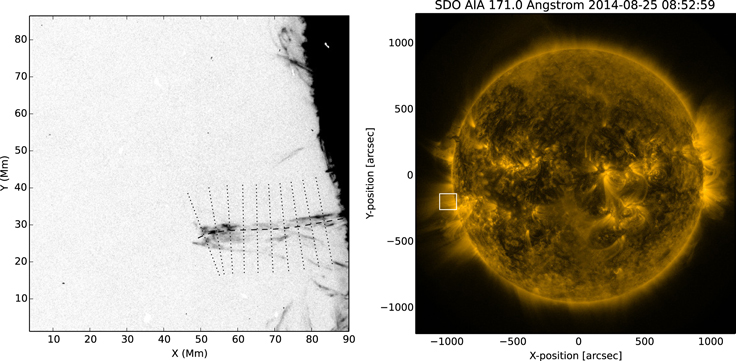
Figure 1. Left: complete field of view of the IRIS Si iv observation used for analysis with the axis of the studied loop outlined. The cuts for the time–distance plots were taken along 10 slits perpendicular to the loop axis. Right: position of IRIS field of view in the full-disk image as seen by SDO/AIA.
Download figure:
Standard image High-resolution imageThe studied loop exhibits a significant amount of coronal rain downflows as well as upflowing material. Most of the upward flow of the plasma occurs in the remote leg while the condensations are falling down preferentially along the loop leg closer to the observer. This asymmetry is likely caused by a background siphon flow due to a pressure difference between the footpoints. Such background flow can move the region where the thermal instability and subsequent condensation occurs to the side away from the apex resulting in coronal rain falling along one leg only.
The view of the observed event is limited to a single vantage point, and we can therefore only make approximate estimates about the loop geometry. The loop plane appears approximately perpendicular to the solar surface. The positions of the axis of the loop, loop apex, and footpoints were determined from a series of multiple SJI time frames superimposed on each other to highlight the flows of the material in the loop. Multiple strands of plasma tracing the loop's magnetic field lines are observed, and the loop therefore appears to have considerable thickness. The radius of the loop was estimated to be 40.9 Mm using the distance from the apex to the loop baseline connecting the two footpoints. Assuming the loop has a semitoroidal shape, the estimate of the loop radius and the observed projected distance between the footpoints of 12.8 Mm was used to estimate the angle between the loop plane and the line of sight to be 9◦.
The plasma condensations falling along the coronal loop are found to have considerable thickness of about 0.5 Mm, often grouping into strands. The individual strands clearly exhibit transverse oscillations which are best visible near the loop apex. The strands were observed to separate and merge again multiple times, thus complicating the tracking of the individual plasma blobs. The most pronounced elongation of the plasma blobs into strands occurs in the lower half of the loop. Individual strands were observed to converge as approaching the loop footpoints.
The longer duration AIA 304 Å data set covering two 12 hr windows before and after the coronal rain event observed by IRIS and Hinode shows that it is a part of a sequence of successive coronal rain events occurring in the same coronal loop. A total of four events were detected on the day of observation. Other events were, however, much less clear due to multiple short-lived rainy loops appearing in the foreground; thus, a detailed analysis of the full 24 hr AIA data set has therefore not been carried out.
3. OSCILLATIONS
In order to detect any transverse oscillations of the structure, we set up 10 slits perpendicular to the loop axis (Figure 1). A cut through data was then taken along each slit and the data was superimposed over 30 pixels in the longitudinal direction to detect oscillations of small blobs as well as of longer strands. The longitudinal superposition length was chosen as being long enough to detect short-strand oscillations and short enough to capture any behavior dependent on the longitudinal distance. The cuts at each time step were then stacked to create time−distance plots, each corresponding to different position along the loop. The time−distance plots created using aligned IRIS Si iv, Mg ii k, and Hinode Ca ii H data show a large degree of similarity with the majority of strand-like structures identifiable in all three wavelengths (Figure 2). This co-spatial emission suggests a multithermal nature of the coronal rain plasma. Time−distance plots created using IRIS Si iv observations corresponding to two slits, one at the loop apex and another 22 Mm above the footpoint are shown in Figure 3. Multiple transverse oscillations are visible along the entire loop length. The contamination lasting from 75 to 85 minutes in the IRIS observational sequence is caused by a surge of particles due to the spacecraft passing through the South Atlantic Anomaly.

Figure 2. Time–distance plots corresponding to slit near the apex in IRIS Si iv (top), Mg ii k (center), and Hinode Ca ii H line (bottom). Hinode data were interpolated to match IRIS time resolution and time range. Co-spatiality of the plasma emission suggest a multithermal nature of the coronal rain. Note the somewhat different features at t = 40–50 minutes captured by Hinode only.
Download figure:
Standard image High-resolution image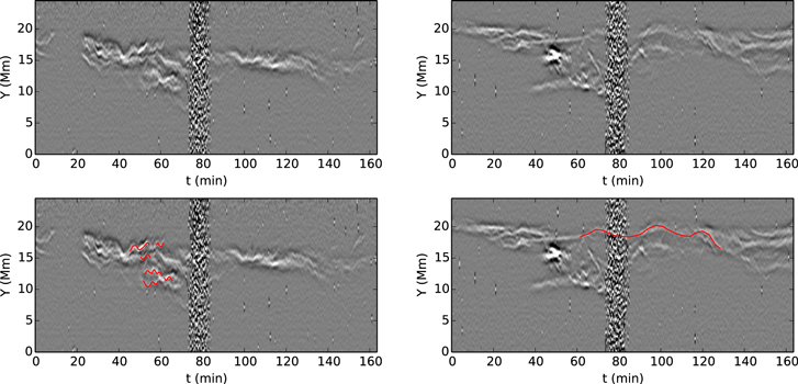
Figure 3. Time–distance plots corresponding to slits near the apex (left) and 22 Mm above the footpoint (right). We repeat both plots with the oscillation patterns highlighted (bottom). Small-scale oscillations are present in both plots. A prominent large-scale oscillating structure is visible only in the lower part of the loop. The particle contamination occurring during 75–85 minutes is due to the spacecraft passing through the South Atlantic Anomaly.
Download figure:
Standard image High-resolution imageDue to the large number of strands present at the same longitudinal distance, traditionally used automated strand detection methods based on fitting a Gaussian to the image intensity profile at each time step (Verwichte et al. 2009, 2010) proved unsuitable. The strand center coordinates were therefore extracted manually from the time–distance plot for each slit to avoid errors that an automated procedure might introduce due to the nature of the intensity profiles. The strand center displacement time series for each oscillation was then extracted and fitted with function  using the Levenberg–Marquardt algorithm in order to determine oscillation parameters. In total, 150 oscillations were observed. The standard deviations on the best-fit parameters for the individual oscillations were found to be 7%, 3%, and 40% for the amplitude, period, and phase, respectively.
The time−distance plots created using IRIS FUV data shown in Figure 3 suggest the presence of two oscillation regimes: short-period oscillations present along the entire loop length but most prominent in the upper part of the loop, and long-period oscillations visible only in the lower half of the loop. We repeat the above analysis using SDO/AIA observations in 171 Å. Due to the 1 5 resolution of SDO/AIA, only the long-period oscillation regime can be observed. Figure 4 shows the variation of the oscillation amplitude with the longitudinal distance of the corresponding slit from the loop apex corrected for the projection effects. There is no clear trend in the amplitude variation; however, the plot shows the distribution of the two populations of oscillations.
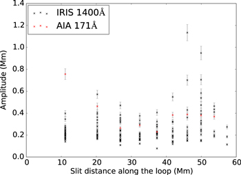
Figure 4. Variation of oscillation amplitude with the longitudinal distance of each slit from the loop apex corrected for projection effects.
Download figure:
Standard image High-resolution imageThe amplitudes of the short-period oscillations were found to mostly lie within a range 0.2–0.4 Mm. No prominent damping of the individual oscillations was observed, although one should note that since only few periods of the individual oscillating strands can be observed, any gradual damping is likely to remain undetected. The mean period of the short-period oscillations was found to be 3.4 minutes. The scatter of the periods of the individual oscillations around the mean value is likely to be a result of the uncertainty on the period measurements. If, despite the measurement errors, this scatter was real, varying periods of the oscillations detected in different positions within the loop would suggest large variations in the properties of the coronal loop plasma. However, due to the fact that a certain level of a collective behavior of individual strands has been observed, we consider this scenario unlikely. A change of the mean oscillation period with time would in turn imply the presence of a non-linear driving process.
Multiple groups of nearby strands were observed to oscillate in phase. Synchronous oscillations were observed to be most prominent in the upper half of the loop. This is likely connected to the fact that only a small number of oscillations was observed near the loop footpoints rather than being a significant evidence of a loss of collective behavior in this part of the loop. There was no significant phase shift detected by comparing different heights, suggesting that the short-period oscillation patterns are a manifestation of a global standing wave. However, the best-fit phase estimates are limited by large uncertainties due to the thickness of the individual strands.
The presence of synchronous oscillations of nearby strands together with the standing wave assumption points toward a number of possible scenarios for the nature of the wave in the coronal loop responsible for the observed oscillation patterns; one such possibility is a global kink mode affecting the coronal loop as a whole. Alternatively, multiple kink modes present in the loop affecting each strand separately could cause in phase transverse oscillating behavior if triggered by a common source. Short-period oscillations traced by the coronal rain with similar characteristics as described above were reported previously (Antolin & Verwichte 2011).
Amplitudes of the long-period oscillations observed in IRIS 1400 Å passband are of the order of 1 Mm. When observing the cool coronal rain plasma emitting at the chromospheric wavelengths, they appear to be most pronounced in the lower part of the loop and fade higher up. At a distance of 37 Mm from the apex, they cannot be observed at all. This is due to the cool plasma being more sparse in the upper part of the loop during the latter half of the observational sequence, which complicates the tracking of long-period oscillatory patterns. In the hot coronal wavelengths, the long-period oscillations are observable along the entire loop length, having similar periods as in IRIS observations but lower amplitudes (Figure 4). This amplitude discrepancy can be attributed to limited resolution of SDO/AIA, with typical peak-to-peak amplitudes of 3 pixels in this oscillation regime. At such short scales, the standard deviation of best-fit oscillation parameters estimated from a sample oscillation pattern might be an underestimate of the true uncertainty. The mean period of this oscillation regime is 17.4 minutes, i.e., much longer than the typical period of the fundamental standing mode of the kink oscillation expected for a loop with comparable length. This suggests that the oscillatory pattern is a manifestation of a propagating rather than standing wave. In the propagating wave scenario, the expected phase shift for such long-period oscillations would be too small to be observed in the data set with this duration.
4. KINEMATICS
The kinematics of the plasma condensations were analyzed by tracking the individual blobs along their paths over the period during which they could be observed in the given bandpass. The individual plasma blobs were best discernible in the data taken in the IRIS Si iv filter, which was therefore chosen for kinematics analysis. Not all plasma blobs were observable during their entire motion from the loop apex all the way to the footpoints; this is likely due to a change in emission in the Si iv line following a temperature change.
By superimposing multiple time frames on each other, we were able to track 18 paths along which the condensations were moving. For each such path, a time–distance plot was extracted. Three such time–distance plots are shown in Figure 5. The bright traces correspond to the trajectories of the individual condensations. A total of 115 plasma blobs were tracked, 18 of which were part of the upflowing material and the remaining 97 blobs were falling condensations. In the subsequent analysis, we focused on the coronal rain blobs. We extracted their trajectories and corrected them for projection effects by calculating the real distance traveled along the loop corresponding to the observed distance of the blob from the apex (assuming 9◦ loop plane angle and semicircular loop axis). For each blob, an initial and final velocity was determined, enabling us to deduce mean acceleration of each blob.
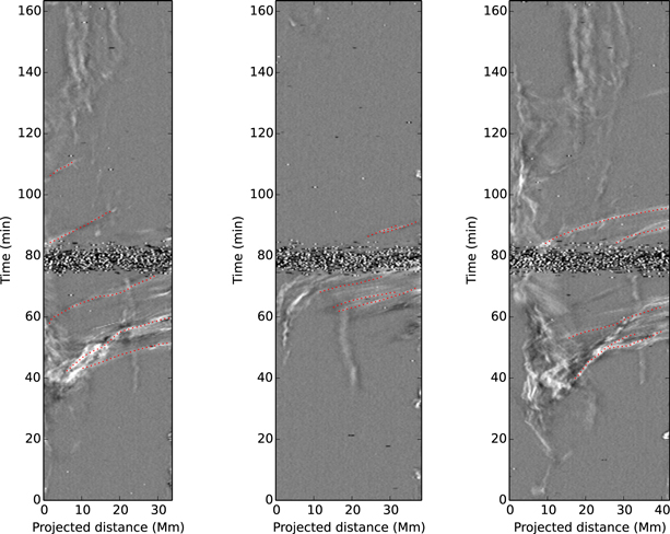
Figure 5. Time–distance plots extracted along three different paths followed by condensations. The horizontal axis corresponds to the projected distance along the path. The bright traces correspond to trajectories of individual blobs. In the rightmost plot, a number of blobs can be observed to oscillate around the loop top before falling down to the solar surface. The faint features stationary in the longitudinal direction are caused by background loops intersecting the axis of the studied coronal loop.
Download figure:
Standard image High-resolution imageThe initial and final velocities and mean accelerations of the coronal rain blobs are shown in Figure 6. The distribution of velocities is broad ranging from small velocities of only few km s−1 to large velocities over 150 km s−1, with the mean velocity being 45 km s−1. The variation of the observed velocity with height is shown in Figure 7. The observed velocities of the individual blobs are largely below free-fall values, shown by the solid line. The distribution of blob accelerations is, on the other hand, much narrower and is clustered around the mean acceleration of 95 m s−2. The average effective gravity along an ellipse is given by  , where s is the coordinate along the ellipse and θ is the angle between the tangent to the path and the vertical. If assuming a semicircular loop axis, the average effective gravity along the loop is 174 m s−2. The measured average acceleration is therefore significantly lower than what would be expected for a free-fall motion. Such sub-ballistic fall rates of coronal rain condensations were reported previously (Schrijver 2001; De Groof et al. 2004; Antolin et al. 2010; Antolin & Verwichte 2011; Antolin & Rouppe van der Voort 2012). Complete velocity and acceleration profiles of individual blobs also show multiple acceleration and deceleration phases as opposed to purely accelerated motion expected if the blobs would be moving solely under the influence of gravity.
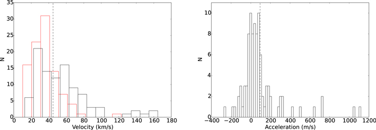
Figure 6. Left: the distribution of blob initial (red) and final velocities (black). Right: the distribution of mean blob accelerations. The dashed lines correspond to the average values of 45 km s−1 and 95 m s−2 for velocities and accelerations, respectively.
Download figure:
Standard image High-resolution image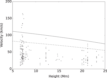
Figure 7. Dependence of blob velocity on the height above the solar surface. The velocity dependence expected for a free-fall motion is shown by the solid line and the velocity dependence expected for a motion with the mean observed acceleration of 95 m s−2 is shown by the dashed line.
Download figure:
Standard image High-resolution image5. HEATING-CONDENSATION CYCLE
In order to determine the temperature evolution of the plasma in the studied coronal loop during the period of observation, we analyze the temporal change in emission in selected SDO/AIA filters. Here we use level 1.5 SDO/AIA data with 12 s cadence normalized by the exposure time, which we aligned with previously analyzed IRIS and Hinode data sets. We select a region of the size 5 × 5 pixels at the loop top, as shown in Figure 8. The normalized emission intensity in each filter is determined by averaging the DN counts over the region of interest and normalizing by the total mean DN counts in each filter. Figure 9 shows the evolution of the total and normalized emission in 94, 131, 171, 193, 211, 304, and 335 Å. The emission first peaks in 94 Å, followed by peaks in 335, 171, 131, and 304 Å, i.e., in progressively cooler bandpasses. It should, however, be noted that low intensities measured in 94 and 335 Å suggest that uncertainties in these light curves are large, thus reducing their reliability. In addition, the lack of a single well defined peak in the instrumental response functions of the 94 and 335 Å channels (Boerner et al. 2011) makes it non-trivial to infer a cooling sequence from the light curves in these two channels. The emission in 193 and 211 Å is, on the other hand, observed to be steadily increasing, with a number of secondary peaks. The sequence of prominent peaks in 171, 131, and 304 Å channels therefore clearly suggests a gradual cooling of the plasma at the loop top, while the emission in the 94, 335, 193, and 211 Å channels does not provide additional evidence of cooling.
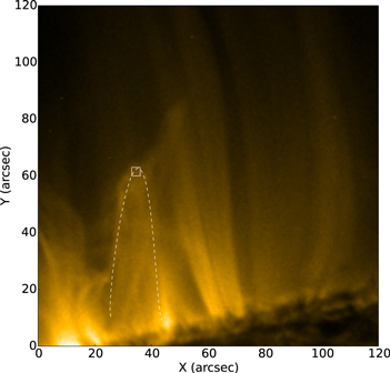
Figure 8. SDO/AIA 171 Å view of the studied coronal loop. The marked region at the loop top used to obtain the evolution of the intensity of the emission.
Download figure:
Standard image High-resolution image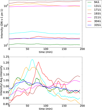
Figure 9. Top: evolution of the observed emission intensities in seven SDO/AIA filters corresponding to the region at the loop top. Bottom: emission intensities normalized by the average number of counts.
Download figure:
Standard image High-resolution imageWe further estimate the temperature distribution of the emission of the loop plasma integrated along the line of sight as a function of time. This can be quantified by the differential emission measure (DEM)  defined as

where ne is the electron density, z is the distance along the line of sight, and T is the temperature. The observed intensities are a result of a convolution of the DEM with the instrumental response functions:

where Fi is the intensity measured in the ith bandpass and Ri is the instrumental response function of the ith filter dependent on the temperature. This can be projected into finite-dimensional space as:

Determining the DEM from the above linear equation, however, poses two main challenges. First, due to the limited number of the instrument bandpasses, the number of the temperature bins of the observed intensities is typically smaller than the number of the temperature bins for which the DEM is evaluated, thus leading to the DEM inversion being an underconstrained problem. Second, the large differences between the magnitudes of the individual components of the response matrix R result in large noise amplification by the inverse mapping. These can be overcome by adding additional constraints to the problem. To do this, we use the zero-order Tikhonov regularization based on selecting the solution with the smallest norm (Tikhonov 1963). This is equivalent to using Lagrange multipliers to solve the least square problem subject to constraints imposed by adding the regularization term:

with Φ to be minimized, λ being the regularization parameter, L being the constraint matrix (proportional to the identity matrix in the case of zero-order regularization), and  being the expected (or guess) solution. This is then solved by diagonalizing the matrices R and L using generalized singular value decomposition, with the
  term in the resulting expression effectively smoothing the solution by filtering out small singular components. To implement the steps above, we use the DEM regularization method by Hannah & Kontar (2012), which we adapted to Python programming language. We run the DEM regularization using the SDO/AIA data in the same bandpasses as above averaged over the region of interest shown in Figure 8. We further averaged the data over 20 time frames to increase signal-to-noise ratio. We reconstruct the DEM for a temperature range between
  and
and  and further apply additional constraint on DEM by requiring it to be positive. Time evolution of the resulting DEM is shown in Figure 10.

Figure 10. Evolution of the regularized DEM plotted every 100 time steps including (left) and (right) excluding the 304 Å channel.
Download figure:
Standard image High-resolution imageThe prominent DEM peak is centered around  . We are most concerned with the DEM evolution below
  , especially with the secondary peak that develops around
  . The amount of plasma in the transition region temperature increases during the first 50 minutes of the observation coinciding with the time interval of the coronal rain occurrence in the upper part of the loop. It should, however, be noted that the validity of the DEM inversion is based on the implicit assumption of the optically thin emission, the resulting DEM evolution in the lower end of the analyzed temperature range should therefore be treated with caution.
Given that the 304 Å channel is most likely to be sensitive to optically thick emission, we repeated the DEM inversion without using the 304 Å channel (Figure 10). This mostly affects the evolution of the low-temperature region, with the early time peak shifted to  . Aside from that the overall shape remains similar. Figure 11 shows the evolution of the DEM integrated along the whole temperature range (representing the evolution of the total amount of plasma at the loop top) and the intensity in the IRIS Si iv time–distance plot corresponding to the slit at the apex (as shown in Figure 3) averaged in transverse direction. The linear correlation coefficients between the Si iv emission intensity and EM recovered with and without using the 304 channel are 0.41 and −0.10, respectively. When including the 304 channel, the overall amount of plasma correlates well with the evolution of the emission in Si iv line, with matching timescales on which the quasi-periodic large-scale variations occur. In the second case, no clear correlation is present. We therefore conclude that due to its broad temperature response, the 304 channel can help to better constrain the DEM in the lower temperature range.

Figure 11. Evolution of the emission measure integrated along the entire temperature range (red) and of the Si iv emission intensity in the time–distance plot corresponding to the slit at the loop apex (blue). The solid and dashed lines show the emission measure recovered with and without using 304 Å channel, respectively. All time series have been smoothed for clarity. The data gap in Si iv emission time series corresponds to the SAA-contaminated data.
Download figure:
Standard image High-resolution imageThe DEM reconstruction and the evolution of the individual light curves together with the occurrence of successive coronal rain events in the same loop suggest that the observed sequence is a part of a continuously repeating heating-condensation cycle, consisting of a heating phase, followed by radiative cooling of the loop top leading to the thermally unstable regime and subsequent condensation of the plasma, which is then followed by another heating phase.
We further verify the above scenario by forward modeling the expected emission intensities in the individual SDO/AIA bandpasses corresponding to a simple heating-cooling process. We created a synthetic time-dependent model of the DEM consisting of two components. The constant background component corresponds to the background emission of the coronal plasma and was modeled using the CHIANTI active region model (Dere & Mason 1993). The low-temperature part (below  ) was removed and the remaining DEM scaled down by an arbitrary factor of 20 to account for the fact that we are modeling an off-limb region. The emission therefore does not contain the low-corona, transition region, and chromospheric elements present in on-disk observation. The foreground component corresponds to the emission of the plasma at the loop top and is time-dependent. We model the foreground DEM as a Gaussian of the form:

where  is the peak emission measure dependent on the electron density and the line of sight integration depth, which we estimate to be of the order of 1 Mm,
  , and
, and  is the mean temperature of the loop plasma. log T0 evolves according to a process consisting of a heating stage characteristic by a linear increase in temperature up to maximum value of
  , catastrophic cooling stage associated with the coronal rain formation where the temperature decreases exponentially and a final gradual cooling stage down to
  (Figure 12). The evolution of the plasma density is modeled in a similar manner to vary linearly between
  and
and  but with the peak slightly delayed, as shown in Figure 12. The initial and peak values were chosen based on typical values expected in active region coronal loops. No direct correlation between the plasma temperature and density is explicitly assumed due to hydrostatic non-equilibrium being the fundamental characteristic of the footpoint-heated loops likely to undergo catastrophic cooling. This evolution effectively marks three distinct phases in the cycle: (1) heating with chromospheric evaporation associated with increasing T and ne; (2) radiative cooling followed by thermal instability and plasma condensation associated with decreasing T and increasing ne; and (3) further cooling accompanied by evacuation of the plasma at the loop top associated with decreasing T and ne.
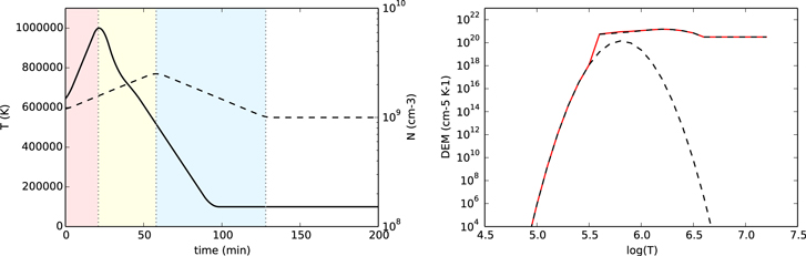
Figure 12. Left: evolution of the mean temperature T0 (solid line) and density (dashed line) of the plasma at the loop top used to generate the DEM model. The colored sections mark the individual phases of the loop thermal cycle: Heating (red), condensation (yellow), and evacuation (blue). Right: the DEM model at t = 0 used to calculate simulated intensities is shown in red. The individual components (constant CHIANTI active region DEM and Gaussian DEM corresponding to the loop plasma) are shown by the dashed line.
Download figure:
Standard image High-resolution imageThe synthetic light curves for each SDO/AIA bandpass are calculated by convolving the composite DEM with the SDO/AIA instrumental response functions (Boerner et al. 2011) using Equation (2). Figure 13 shows the absolute modeled emission intensities and the intensities normalized by the average value in each bandpass for the sake of easy comparison with the observed values. Large-scale characteristics, average values, and amplitude of variations in the observed emission intensities are generally in good agreement with those predicted for the heating-cooling cycle with the given temperature and density evolution. The average observed emission intensities in the 193 and 211 Å bandpasses are, however, higher than predicted; this is likely is caused by the fact that the background model used here underestimates the emission in hot coronal wavelengths for the observed region. As with the observed intensities, a clear signature of gradual cooling of the plasma in modeled evolution of the emission is present, consisting of the emission peaking in subsequently cooler bandpasses. As mentioned above, the emission in 193 and 211 Å is observed to gradually increase, with a number of smaller secondary peaks present, which is in disagreement with the single peak in each bandpass predicted by the model. This can be attributed to the temperature of the background coronal plasma steadily increasing. Such evolution could be expected, e.g., for a bundle of thermally unstable loops in the background that are also going through the heating phase of the heating-condensation cycle but with the instability timescale being longer (e.g., due to longer loop length). This is further supported by the fact that the multiple prominent peaks in the 193 and 211 Å are each accompanied by secondary peaks in other bandpasses, which are not exactly co-temporal due to the expected temperature change. The observed evolution is therefore likely a result of superposition of multiple cooling/heating sequences in the foreground/background. The simulated emission peaks in 171, 131, and 94 Å are narrower than observed and the decay of all light curves is more rapid than observed. Here it should be noted that the DEM model used is valid for a monolithic loop. The multithermal structure of the coronal loop would result in emission peaks of greater width, in line with the observations. Considering above limitations of the background model and the fact that at lower temperatures the plasma is likely entering the optically thick regime, the forward modeling approach should be viewed as a demonstration of the feasibility of the limit cycle model given the observed light curve evolution rather than as a direct reproduction of the observations.

Figure 13. Comparison of the observed (left) and simulated emission intensities based on a two-component DEM model corresponding to a simple heating-cooling process (right). The linear trend from the observed emission in the 193 and 211 Å channels has been removed. Bottom panels show the emission intensities normalized by the average number of counts. The colored sections mark the individual phases of the loop thermal cycle: Heating (red), condensation (yellow), and evacuation (blue).
Download figure:
Standard image High-resolution image6. DISCUSSION
There are a number of possible sources that could potentially be responsible for the two distinct oscillation regimes with different periods. The 3.4 minute average period characteristic for the small-scale oscillation regime is consistent with the period of the fundamental standing mode  ∼3 minutes if using typical estimate for the Alfvén speed (∼1000 km s−1) and loop length determined previously (129 Mm). The absence of observable damping in the small-scale case suggests the presence of a continuously operating non-resonant driver. The mean period of the large-scale oscillation regime is much longer than one expected for the fundamental harmonic and therefore cannot be associated with the standing mode scenario, suggesting the agent instead being a propagating wave. Here the intermittent nature of the oscillations implies localized, transient driving mechanism operating near the footpoints of the coronal loop.
Most prominent sources of the MHD waves in the corona are solar flares and other energetic events, which can be observed in a number of passbands (radio, UV, X-ray) as well as in the particle flux measurements. Such events were found to excite transverse oscillations in the coronal loops with the periods on the order of minutes (Aschwanden et al. 2002; Nakariakov et al. 2009), matching the timescale of the small-scale oscillation regime observed and discussed in this work. However, event-triggered loop oscillations usually exhibit strong damping and were found to typically decay within few oscillation periods (Nakariakov et al. 1999; White & Verwichte 2012), unlike the oscillations described here. There were no detected flares or other energetic events occurring on the date of the observation near AR 12151. An M class flare occurred in this active region during the previous day and a series of C class flares was observed in AR 12149 and AR 12150 on the day of observation; however, these were perceived as being too distant to have a significant effect on the studied coronal loop. The limited STEREO-A data set available for the day of observation was also checked to exclude the possibility of a nearby flare occurring behind the limb.
The persistent nature of the small-scale oscillations and their lack of observable decay instead suggests that there is a possible link with the decayless transverse oscillations of coronal loops in non-flaring active regions having similar characteristics which were observed at EUV wavelengths (e.g., Nisticò et al. 2013). If the small-scale oscillation regime is indeed a manifestation of the same process as these decayless loop oscillations, the common occurrence of this phenomenon implies a global nature of the driving mechanism, possibly a stochastic driver (e.g., small-scale reconnection events or stochastic motions in the chromospheric network resulting from granular flows). Another possibility is a global helioseismic p-mode coupling to the loop footpoints. Because of the large number of other loops in the vicinity of the studied coronal loop, the possibility of an interaction with neighboring loops has to be taken into account. Assuming that their proximity is not just a projection effect, interaction with the neighboring loops could perturb the conditions in the studied loop and trigger both condensation region formation and transverse loop oscillations. It has also been suggested that if the inertia of the coronal rain blobs is not negligible, the condensations themselves could excite the oscillations in the loop. A detailed analysis of this scenario will be addressed in the future work.
The reasons behind sub-ballistic fall rates of the coronal rain blobs are less clear and are subject to ongoing discussion. Gas pressure gradients in the loop are thought to have strong effect on the dynamics of plasma condensations. As the condensation falls down along the magnetic field line, it compresses the plasma below. The resulting strong pressure could slow down the blob significantly. Numerical simulations show that these pressure effects can be strong enough to account for some of the observed deceleration (Müller et al. 2005; Fang et al. 2013; Oliver et al. 2014). The motion of the blobs would also appear sub-ballistic if the blobs would be moving along paths resulting from helical structure of magnetic field lines. Such helical configuration of the magnetic field would, however, need to be stable for extended periods of time, which we consider unlikely. Another factor that needs to be considered is the PMF exerted by the transverse oscillations in the loop. The PMF can be directed either along or against the direction of the motion of the condensations depending on their position along the loop and on the harmonic of the transverse standing wave in the loop. This would provide an explanation of the multiple acceleration and deceleration phases in the blob motion. The scenario that the coronal rain evolution is at least partially affected by the PMF is further supported by the fact that a number of coronal rain blobs were observed to oscillate around the loop top, as shown in Figure 5. A model of the effect of the PMF on the kinematics of the coronal rain has already been proposed (E. Verwichte et al. 2016, in preparation). The influence of the PMF on the coronal rain kinematics will be addressed in detail in the future work.
Our observations of the thermal evolution of the plasma in the studied coronal loop are consistent with the limit cycle model, where steadily heated loops are expected to undergo periodically repeating cycles consisting of heating and condensation phases with periods on timescales of hours, typically dependent on the loop length and the shape of the heating function. A possibility of cyclic evolution of coronal loops was first addressed by Kuin & Martens (1982), who obtained an oscillatory solution if the strength of the coupling between the coronal loop and the chromosphere was lower than a critical value, using a relatively simple semi-analytical model based on modeling the loop as a zero-dimensional system. Their model was further generalized by Gomez et al. (1990) by fully accounting for the hydrodynamic considerations whose solution has the form of subcritical Hopf bifurcation. These models are, of course, highly simplified and use average values of the temperature and density along the loop, and hence do not account for a variation in the spatial distribution of the heating function, which we now know is an important factor that determines the thermal instability onset. They can, however, still be used for the prediction of the general behavior of the system since they account for key ingredients of the heating-condensation cycle: chromospheric evaporation, catastrophic cooling, and subsequent evacuation of the loop. The limit cycle behavior has been also predicted by a number of numerical studies (e.g., Karpen et al. 2001; Müller et al. 2003; Fang et al. 2015).
Considering an idealized temperature-density limit cycle similar to the oscillatory solution of Kuin & Martens (1982), we expect presence of four different stages of the loop evolution in one cycle period (Figure 14): a heating phase associated with increasing temperature and density due to the chromospheric evaporation of the plasma into the loop; a radiative cooling phase associated with the rapid cooling and subsequent condensation of the plasma at the loop top, resulting in decreasing temperature and increasing density; a gradual cooling phase accompanied by the evacuation of the loop top as the coronal rain plasma falls toward the solar surface, thus decreasing in the plasma density; and the final reheating phase where the density continues to decrease and the heating starts again. It can be immediately seen that the first three stages of the expected limit cycle behavior are in agreement with the evolution of the plasma density and temperature deduced by the forward modeling of the observed emission intensities carried out in this study. It should be noted that when looking at the evolution of the observed emission intensities alone, only the cooling part of the heating-condensation cycle has clear observational evidence (i.e., sequential peaks in progressively cooler bandpasses), given the lack of a simple observational signature of the presence of a heating phase immediately preceding the cooling of the loop plasma. The deduced effect of adding the heating phase on the onset of cooling progression when forward modeling the emission intensities seems to be in line with the observations. This, together with the repeated coronal rain occurrences in the same coronal loop, supports the complete heating-condensation cycle scenario.

Figure 14. Phase diagram of the loop evolution deduced from forward modeling the SDO/AIA emission intensities. The dashed line shows extrapolated evolution prior to the start of the observational sequence.
Download figure:
Standard image High-resolution image
Whereas the resulting DEM evolution calculated using the regularization method is in agreement with the results deduced using the forward modeling approach, care must be taken with the interpretation of the thermal evolution of the plasma in the lower end of the analyzed temperature range, where it is likely entering the optically thick regime. In addition, contamination of the emission from the studied region by the emission of the hot coronal background seems to be an ongoing problem. In order to evaluate the degree to which the DEM determined in this work is affected by the coronal background, it should be pointed out that due to the greater column depth, the contamination by the background emission is likely to be more severe near the solar limb than near the center of the solar disk, where the DEM is usually much more accurate (e.g., Warren et al. 2010; Hannah & Kontar 2012). Since the coronal rain is best observed off-limb, this poses a challenge for the extraction of the relevant information about temperature evolution of the studied coronal loop. The background subtraction was not carried out in this work, as it proved impossible to select a reference area where the average intensity in the most noisy channels (94 and 335 Å) would be less than the average value in the analyzed region in all time frames. An alternative approach would be to simply exclude these two channels from the analysis. However, this was viewed as undesirable due to the fact that it would lead to the DEM being even more underconstrained. Including the effect of the hot coronal background and tackling the problem using the forward modeling therefore seems to be the most viable approach for the off-limb regions. However, as shown by this work, the steady background model has its limitations, since a change in the background temperature during the period of the observation (e.g., due to a bundle of loops undergoing similar heating-cooling cycles, but with longer cycle periods) is entirely possible.
The change of plasma density near the loop top resulting from the chromospheric evaporation and subsequent condensation is expected to have an effect on the Alfvén speed in this part of the loop. For the change in density by a factor of 2.5 as estimated in the previous section, the Alfvén speed  is expected to change by a factor of 1.6. With
  and
and  , this decrease in density will result in a decrease in the oscillation period by a factor of 1.6 and vice versa. The observed scatter in the period of the oscillations traced by the coronal rain blobs could therefore be partially caused by the density change due to evacuation of the loop top.
7. CONCLUSIONS
We analyzed transverse oscillations and kinematics of coronal rain observed by IRIS, Hinode/SOT, and SDO/AIA. Two different regimes of transverse oscillations traced by the rain in the studied coronal loop were observed: small-scale oscillations with a mean period of 3.4 minutes and amplitudes between 0.2 and 0.4 Mm that can be observed along the entire loop length, and large-scale oscillations with a mean period of 17.4 minutes and amplitudes around 1 Mm, observable only in the lower part of the loop. The small-scale oscillations are visible during most of the duration of the data set without any observable damping, and they are therefore likely driven by a continuously operating process. The collective behavior of the individual oscillating strands and lack of phase shift suggests they correspond to a standing wave excited along the whole loop. The 3.4 minute period of this oscillation regime is consistent with the period expected for a fundamental harmonic of the loop with similar length. The large-scale oscillations are only visible in the latter half of the observational sequence. The unusually long period suggests a propagating wave scenario, where the wave is excited by a transient mechanism localized near the loop footpoints.
Plasma condensations were found to move with speeds ranging from few km s−1 up to 180 km s−1 and with accelerations that were largely below the free-fall rate. The broad velocity distribution, sub-ballistic motion, and complex velocity profiles of individual blobs showing multiple acceleration and deceleration phases suggest that forces other than gravity have a significant effect on the evolution of the coronal rain, the likely candidates being pressure effects and the PMF caused by the transverse loop oscillations.
The observed evolution of the emission in individual SDO/AIA bandpasses was found to exhibit clear signatures of a gradual cooling linked to the formation of plasma condensations. The temperature evolution of the plasma was examined in more detail using DEM regularization technique and by forward modeling the emission intensities in the SDO/AIA bandpasses using a two-component DEM model dependent on the evolution of the temperature and density of the plasma near the apex of the coronal loop. The inferred evolution is consistent with the limit cycle model of the coronal loop and suggests the loop is going through a sequence of periodically repeating heating-condensation cycles.
P.K. acknowledges the support of the UK STFC PhD studentship. E.V. acknowledges financial support from the UK STFC on the Warwick STFC Consolidated Grant ST/L000733/I. We would like to thank P. Antolin, G. Vissers, and D. Yuan, the co-observers during the 2014 August observing campaign at SST. This research has made use of SunPy, an open-source and free community-developed solar data analysis package written in Python (http://sunpy.org). IRIS is a NASA small explorer mission developed and operated by LMSAL with mission operations executed at the NASA Ames Research Center and major contributions to downlink communications funded by the Norwegian Space Center (NSC, Norway) through an ESA PRODEX contract. Hinode is a Japanese mission developed and launched by ISAS/JAXA, with NAOJ as a domestic partner and NASA and STFC (UK) as international partners. It is operated by these agencies in cooperation with ESA and NSC (Norway). The SDO/AIA data are available by courtesy of NASA/SDO and the AIA, EVE, and HMI science teams. The work was also supported by the international programme "Implications for coronal heating and magnetic fields from coronal rain observations and modeling" of the International Space Science Institute (ISSI), Bern.