


ABSTRACT
A recent study discussed the steady-state model for solar wind electrons during quiet time conditions. The electrons emanating from the Sun are treated in a composite three-population model—the low-energy Maxwellian core with an energy range of tens of eV, the intermediate ∼102–103 eV energy-range ("halo") electrons, and the high ∼103–105 eV energy-range ("super-halo") electrons. In the model, the intermediate energy halo electrons are assumed to be in resonance with transverse EM fluctuations in the whistler frequency range (∼102 Hz), while the high-energy super-halo electrons are presumed to be in steady-state wave–particle resonance with higher-frequency electrostatic fluctuations in the Langmuir frequency range (∼105 Hz). A comparison with STEREO and WIND spacecraft data was also made. However, ignoring the influence of Langmuir fluctuations on the halo population turns out to be an unjustifiable assumption. The present paper rectifies the previous approach by including both Langmuir and whistler fluctuations in the construction of the steady-state velocity distribution function for the halo population, and demonstrates that the role of whistler-range fluctuation is minimal unless the fluctuation intensity is arbitrarily raised. This implies that the Langmuir-range fluctuations, known as the quasi thermal noise, are important for both halo and super-halo electron velocity distribution.
Export citation and abstract BibTeX RIS
1. INTRODUCTION
The charged particles have been detected by artificial satellites since the beginning of the age of in situ space exploration. The discovery that their velocity distribution functions (VDFs) deviate substantially from the thermal equilibrium form was unexpected, whose origin is, to this day, not completely understood. As far as the electrons measured near 1 au are concerned, it is customary to phenomenologically treat these charged particles as three or four distinct components. The dominant components are the quasi-isotropic core electrons that make up to 95 ∼ 96% in terms of the total number density. The core electrons are characterized by tens of eV thermal energy (or ∼103 km s−1 thermal speed). The next prominent component is the intermediate energy electron population, which make up to roughly 4%–5% in number density. These electrons have thermal energy in the range of ∼102 to 103 eV, or equivalently, ∼4 × 10³–104 km s−1 thermal speed. These are known as the halo component. Typically, the halo component is modeled by a non-thermal distribution featuring an energetic tail, i.e., the kappa distribution (Vasyliunas 1968), whereas the core electrons are adequately modeled by the Maxwellian model. The halo electrons can possess a net drift with respect to the core electrons such that these electrons can be the source of a substantial heat flux. In general, electrons are important in the dynamics of the solar wind, not only for maintaining the charge neutrality and large-scale electrostatic (ES) field generation, but also for contributing to the overall heat flux.
The third electron component is a highly field-aligned "strahl" that is observed to be streaming away from the Sun. The strahl is more prominent in the fast solar wind, and their energy range overlaps with that of the halo. Observation shows that a potential inter-relationship between the strahl and the halo electrons may exist. On the basis of a statistical analysis of Helios, Cluster II, and Ulysses spacecraft data, Maksimovic et al. (2005) and Štverák et al. (2009) demonstrated that the relative number of the strahl electrons decreases with the radial distance from the Sun, whereas that of the halo electrons increases, thus indicating the possibility of the strahl electrons pitch-angle scattering into the halo. In a recent letter, however, Seough et al. (2015) propose that the strahl may not even be a separate population, but rather it may simply give the appearance of being a field-aligned beam as a result of a complicated wave–particle interaction between the halo and core with a net relative drift and temperature anisotropy. The localized distortion of the velocity space distribution function (VDF) for the halo electrons leads to the semblance of a field-aligned beam. It is more customary, however, to model the strahl and halo as separate components. We are not concerned with the strahl component in the present paper, however.
The fourth component is the highly energetic "super-halo" component, with thermal energy in the range of ∼103–105 eV, or equivalently, ∼104–105 km s−1 thermal speed. The number density of the super-halo is extremely low, typically 10−9–10−6 of the total density, but their presence is easily recognizable in VDF. For general overviews of observations and discussions of various aspects referenced above see the following articles: Montgomery et al. (1968), Vasyliunas (1968), Lin (1973, 1998), Feldman et al. (1975), Rosenbauer et al. (1977), Pilipp et al. (1987a, 1987b), McComas et al. (1992), Lin et al. (1995), Hammond et al. (1996), Fitzenreiter et al. (1998), Maksimovic et al. (2000, 2005), Salem et al. (2003a, 2003b), Štverák et al. (2009), and Wang et al. (2015).
A recent series of papers put forth a steady-state model of the solar wind electrons during quiet time solar wind conditions (Kim et al. 2015; Yoon et al. 2015). According to this model the Maxwellian core electrons do not resonate with any plasma waves, thus remaining in the essential Maxwellian state, but the model envisions the intermediate energy halo electrons constantly exchanging momentum and energy with the whistler frequency range transverse fluctuations, while maintaining a dynamical steady state. The source of the whistler fluctuation is assumed to be the spontaneous thermal emission and re-absorption by the halo electrons. The reason for considering the whistler fluctuation was motivated in part by previous theoretical works that emphasized the role of whistler turbulence in the halo and strahl electron dynamics (Vocks et al. 2005; Gary & Saito 2007; Saito & Gary 2007a, 2007b; Pierrard et al. 2011), and also by the recent observation of whistler fluctuations in the solar wind (Lacombe et al. 2014). The solar wind is characterized by permanent low-frequency turbulence, whose high-frequency part of the spectrum in the spacecraft frame is often interpreted as the whistler frequency range. However, as noted by Lacombe et al. (2014), such a feature may be a consequence of a Doppler frequency upshift, and the actual frequencies in the solar wind frame may be too low to satisfy the cyclotron resonance condition with the electrons. In contrast, the spontaneously emitted whistler spectrum is of a different kind whose frequency is in the true whistler frequency range in the solar wind frame. Kim et al. (2015) and Yoon et al. (2015) invoked such a self-generated whistler-range fluctuation spectrum. In the quasi-asymptotic stage, Kim et al. (2015) showed that the steady-state solution of the particle kinetic equation for halo VDF is given by
where C is the normalization constant, me and c stand for the electron mass and the speed of light in vacuo, respectively, and the quantity km is the maximum perpendicular wave number associated with the spontaneously emitted whistler wave fluctuation, which can be taken to be on the order of inverse thermal electron gyroradius,  , vTh being the electron thermal speed (Gaelzer et al. 2015). In Equation (1) the quantity
  is the cosine of the pitch angle, α; the electron gyro-frequency, Ωe, and the plasma frequency, ωpe, are define by
  and
and  , respectively. Here, e denotes the unit electric charge. Quantities B0 and n0 designate the ambient magnetic field intensity and the total electron number density, respectively. In the present paper,
  and
and  are velocity components perpendicular and parallel to the ambient magnetic field, respectively. Note that the steady-state VDF (1) contains the stationary whistler electric field fluctuation spectrum
  evaluated at the resonant wave number

Consequently, the formal solution (1) requires the knowledge of the wave intensity, which is discussed in the subsequent paper Yoon et al. (2015), where the authors showed that the stationary whistler wave spectral intensity is given by
where  . The formal solution (2) contains the halo electron VDF and its derivative evaluated at the resonant velocity

The coupled Equations (1) and (2) thus constitute the self-consistent solar wind halo model.
Kim et al. (2015) and Yoon et al. (2015) demonstrated that the kappa VDF, and associated whistler wave fluctuation spectrum given below, form an approximate pair of self-consistent steady-state solutions to Equations (1) and (2),
Here, nh is the halo electron number density. In the above equation the kappa parameter, κh, is a freely adjustable parameter, but observations show that it is close to six to eight. We shall choose κh = 8 henceforth. The quantity  is the thermal speed associated with the halo electrons, Th being the halo temperature. Since the whistler fluctuation is a transverse mode, there exists magnetic field fluctuation intensity,
We reiterate that the above solutions (3) and (4) are approximate. In fact, according to (Kim et al. 2015), who derived the solution from the perspective of particle equation, the wave spectrum has an undetermined parameter, H, associated with the last term within the large parenthesis on the right-hand side of the expression for  , namely, the last term is given by
 ![$1/\left[\left({\kappa }_{h}-\tfrac{3}{2}\right)H\right]$](https://content.cld.iop.org/journals/0004-637X/826/2/204/revision1/apjaa2ac4ieqn11.gif) . Similarly, the wave spectrum discussed in the paper by Yoon et al. (2015), where the problem is approached from the standpoint of wave equation, also contained an undetermined parameter associated with the whistler wave spectrum. Specifically, in the case of Yoon et al. (2015), the undetermined H parameter multiplies the entire expression within the large parenthesis, i.e.,
. Similarly, the wave spectrum discussed in the paper by Yoon et al. (2015), where the problem is approached from the standpoint of wave equation, also contained an undetermined parameter associated with the whistler wave spectrum. Specifically, in the case of Yoon et al. (2015), the undetermined H parameter multiplies the entire expression within the large parenthesis, i.e., ![$\left[{k}^{2}{v}_{\mathrm{Th}}^{2}/{{\rm{\Omega }}}_{e}^{2}+1/\left({\kappa }_{h}-\tfrac{3}{2}\right)\right]{H}^{-1}$](https://content.cld.iop.org/journals/0004-637X/826/2/204/revision1/apjaa2ac4ieqn12.gif) . In the present paper we simply choose these undetermined parameters as unity. As discussed by Yoon et al. (2015), mathematically exact solutions for the coupled Equations (1) and (2) are not generally forthcoming except in two special cases, namely, the Gaussian VDF and an inverse power law VDF. Note that the kappa VDF approaches the Gaussian form for low energy while it asymptotically forms the inverse power law VDF for high velocity. In this sense the model (3) is sufficiently accurate to serve as a possible halo model.
. In the present paper we simply choose these undetermined parameters as unity. As discussed by Yoon et al. (2015), mathematically exact solutions for the coupled Equations (1) and (2) are not generally forthcoming except in two special cases, namely, the Gaussian VDF and an inverse power law VDF. Note that the kappa VDF approaches the Gaussian form for low energy while it asymptotically forms the inverse power law VDF for high velocity. In this sense the model (3) is sufficiently accurate to serve as a possible halo model.
As we shall discuss, however, the solution (3), while useful since it is given in mathematically closed form, turns out to be incomplete since the fundamental assumption of the halo electrons interacting exclusively with the whistler turbulence does not provide an accurate picture. It will be shown that the Langmuir fluctuation is far more influential than the whistler fluctuation for the halo electrons. The purpose of the present paper is to present a revised model of the halo electron VDF. The above discussion is necessary to provide the backdrop for the present paper. Before we discuss the details of the revised model, let us further review the previous works for the sake of completeness.
Kim et al. (2015) and Yoon et al. (2015) also considered the mutual relationship between the Langmuir fluctuation and super-halo electrons, the analysis of which is similar to the whistler-halo solution, except that the Langmuir fluctuation is longitudinal. The self-consistent set of formal equations are similar to (1) and (2), except that now the Langmuir fluctuation is involved and the electron species under question is a super-halo. The coupled formal solutions are given by
Note that resonant wave number and velocity are now given by  and
and  , respectively. Thermal emission of Langmuir fluctuations is well known, and it is called the quasi thermal noise in the literature (Meyer-Vernet 1979; Meyer-Vernet & Perche 1989; Zouganelis 2008; Le Chat et al. 2009). An earlier analysis by Yoon (2014) actually described in detail, already, how a single-component electron VDF attains the form of kappa distribution when these electrons interact with quasi thermal noise. The analyses by Kim et al. (2015) and Yoon et al. (2015) that pertain to the super-halo and Langmuir fluctuation are essentially the same as that of Yoon (2014), except that they reconsidered the problem in the context of multi-component electrons. Kim et al. (2015) and Yoon et al. (2015) constructed an approximate but reasonably accurate model of the super-halo electrons and the associated quasi thermal noise spectrum as follows:
In Equation (6) the kappa index of κs = 2.25 is chosen following the analysis by Yoon (2014). The quantity ns is the super-halo number density, while  stands for the thermal speed for super-halo electrons, Ts being the super-halo temperature, and
  represents the thermal speed for the Maxwellian core electrons. Here, Te is the core electron temperature. The reason why the core electron temperature enters in the model of the Langmuir fluctuation spectrum is because the dense core electrons determine the wave dispersive properties. We will not be concerned with the super-halo VDF in the present paper, as the model (6) is quite accurate and is based on firm theoretical as well as observational justification (Wang et al. 2012; Yoon 2014). Kim et al. (2015) compared the theoretically constructed solution to actual solar wind electron data obtained via STEREO and WIND spacecraft, and a reasonable comparison was achieved, or at least it was thought that the good comparison provided the justification for the model. In hindsight, however, our comparison turned out to be not much more than just fitting the data with model distributions with appropriate input parameters. However, it should be noted that (Kim et al. 2015) did after all provide a theoretical justification in the model distributions, such as kappa VDF are possible under suitable wave turbulence spectra.
Our main concern in the present paper is to revisit and revise the halo electron model. One of the shortcomings of the earlier model is the artificial delineation of the non-thermal electron VDF into halo and super-halo components. It is desirable to discuss the total non-thermal electron VDF as a single component model. Such a task is the subject of a future paper. The present concern is on an even more restrictive assumption. That is, the ad hoc restriction of exclusive resonance between whistler fluctuation and halo electrons, while ignoring the contribution of Langmuir fluctuations. The similarly selective assumption of and exclusive resonance between the super-halo electrons and Langmuir fluctuations is not that bad, however, since the super-halo range of non-thermal electrons actually do not effectively resonate with the intermediate frequency whistler fluctuations. The real problem is with the halo model. In general, there is no a priori reason why the halo electrons should interact with the whistler waves only. Kim et al. (2015) and Yoon et al. (2015) simply argued on the basis of resonance conditions, which shows that the halo electrons favorably interact with whistler waves, while the super-halo electrons preferentially satisfy the Langmuir wave resonance criterion.
However, a recent paper by Kim et al. (2016) investigates the fundamental properties of spontaneously emitted ES and electromagnetic fluctuations by the electron VDF composed of core, halo, and super-halo populations. To recapitulate the discussion by Kim et al. (2016), the electric field spectral intensity associated with the spontaneous emission is given by
where nc and n0 represent the core and total electron densities, respectively, vTe being the core thermal speed. Note that in evaluating the linear dielectric response functions,  and
and  , Kim et al. (2016) ignored contributions from non-thermal electrons. However, their contribution to the "source" fluctuation is fully kept. In Equation (7), Z(ζ) is the plasma dispersion function, and the source fluctuation intensities are defined by
The contributions to the source fluctuation that comes from the Maxwellian core electron are the first terms within large square brackets on the right-hands, while the second terms contain non-thermal electron contributions. The non-thermal electron source terms are computed on the basis of kappa VDF models.
Figure 1 plots the spontaneously emitted electric field spectrum,  , as well as the magnetic field spectrum,
  . The panels on the left show the electric field spectrum while the right-hand panels depict the magnetic field spectrum. Note that the E field contains both the transverse and longitudinal polarizations, and we did not distinguish between the two. In plotting the results shown in Figure 1 we assumed ωpe/Ωe = 50, nc/n0 = 0.96, nh/n0 = 0.039999 (∼4% halo density), ns/n0 = 10−6, vTe/c = 0.006, vTh/c = 0.0136, vTs/c = 0.0375, κh = 8, and κs = 2.25. These physical input parameters are consistent with typical solar wind conditions near 1 au during quiet time, and are in fact consistent with those adopted in the paper by Kim et al. (2015). Top two panels depict the total electric and magnetic field spectra where all three electron components, core, halo, and super-halo, are taken into account in computing the source fluctuations. The Langmuir (L) and whistler (W) dispersion relations are superposed with dashed curves. As one can see, these collective plasma eigenmodes show enhancements (see the color bar for dimensionless relative intensity in logarithmic scale). The middle panels show the field spectra by taking into account only the halo contribution in the source fluctuation. Note that the enhanced emissions along the eigenmodes are virtually identical to the total field spectra, indicating that the halo electrons dominate the spontaneous emission even though they constitute only 4% in number density. The bottom two panels plot the contribution from the super-halo population only. Note that the super-halo electrons contribute somewhat to the Langmuir mode fluctuation but virtually nothing to the whistler mode fluctuation.

Figure 1. Spontaneously emitted electric field spectrum,  (left columns), and the magnetic field spectrum,
  (right-hand panels). The top two panels depict the total electric and magnetic field spectra where all three electron components, core, halo, and super-halo, are taken into account. The middle panels show only the halo contribution. The bottom two panels plot the contribution from the super-halo population only. Note that the halo electrons dominate the spontaneous emission even though they constitute only 4% in number density. Note also that the super-halo electrons contribute somewhat to the Langmuir mode fluctuation but virtually nothing to the whistler mode fluctuation.
Download figure:
Standard image High-resolution imageJudging from Figure 1, and according to Kim et al. (2016), the halo electrons emit not only the whistler-range fluctuations but also the higher-frequency Langmuir fluctuations. The super-halo electrons, on the other hand, largely contribute to Langmuir fluctuation only. The fact that the halo electrons contribute equally to the emission of whistlers and Langmuir waves implies that the reverse must also be true. That is, both whistlers and Langmuir waves must be equally absorbed by the halo electrons so as to lead to steady-state non-thermal VDF. The artificial restriction of halo electrons resonating only with whistlers must therefore be fundamentally re-examined. This realization has prompted the present authors to revisit the previous model of the steady-state solar wind halo electron model. In what follows, we systematically expound on the general model in which both whistlers and Langmuir fluctuations are incorporated in the construction of the steady-state VDF, and we will examine the relative importance of the two types of fluctuations on the electrons. Note that the assumption of a super-halo interacting solely with the Langmuir fluctuation is valid, as evidenced by the bottom two panels of Figure 1.
2. GENERALIZED HALO ELECTRON VDF
Let us consider the general asymptotically steady-state solution for the electrons already derived in (Kim et al. 2015),
In the above,  is the transverse dielectric constant while
  designates the longitudinal dielectric constant.
  and
and  are the wave electric field spectral intensity corresponding to the right-hand circularly polarized transverse fluctuation and the longitudinal fluctuation, respectively. If we assume that the electric field intensities are determined by the collective eigenmodes, that is, whistler and Langmuir modes, then we may simplify the analysis by eliminating the ω integral by virtue of the dispersion relations. Note that the coefficients A(v) and D(v) contain contributions from both cyclotron resonance delta function,
  , and Landau resonance delta function,
  , as well as contributions from transverse wave intensity,
  , and longitudinal wave intensity,
  . The earlier approximation pertains to ignoring one type of resonant interaction and wave intensity versus the other when dealing with either halo or super-halo populations. In the revised model we will keep the full expressions for A(v) and D(v) without ignoring one term over the other. We are particularly interested in the revised halo model since, according to Kim et al. (2016), the spontaneously emitted whistler and Langmuir fluctuation intensities are dominated by contributions from the halo electrons.
The strategy of the revised halo electron modeling is as follows: We start from the model VDF fh(v) given by the first equation in (3), which is analytically expressed in the form of kappa distribution. This constitutes the initial model. We then make use of the initial model to compute the wave intensity. In doing so, however, instead of making use of the whistler fluctuation intensity  , which is given by the second equation in (3), we directly compute both the whistler and Langmuir fluctuation intensities on the basis of a more general spontaneous emission formula found in the paper by Kim et al. (2016). That is, we will recalculate the collective mode spectrum on the basis of Equations (7) and (8). The reason is because the whistler spectrum given by the second equation in (3) is approximate in the sense that the wave frequency is assumed to be sufficiently lower than the electron gyro-frequency,
  . Moreover, the Langmuir intensity spectrum is absent in Equation (3). In contrast, the spontaneous emission formula derived in Kim et al. (2016), namely, Equations (7) and (8), is more general, since these equations do not make the assumption
  on the whistler spectrum, and the formula also contains the Langmuir intensity spectrum as well. The next step in the procedure is to make use of whistler and Langmuir spectra in the coefficient D(v) in Equation (9). Together with the general expression for A(v), which contains both cyclotron and Landau resonances, we will directly (re)calculate fh(v) by numerically integrating the indefinite velocity integral—the first equation in (9). Ideally, the improved model should not deviate too much from the initial model, and in fact, as we will shortly see, the deviations are not too severe. We could, in principle, iterate the above procedures as many steps as possible in order to improve the numerical accuracy, but doing so unnecessarily complicates the main thrust of the present purpose. Recall that the present purpose is to examine the relative roles of the whistler versus Langmuir fluctuation intensities in the halo VDF. The advantage of the above-outlined modeling effort is that the outcome contains contributions from both whistler and Langmuir fluctuation intensities, as well as both types of wave–particle resonance conditions in relative obvious expressions, as we will see, so that we may diagnose the contribution from each wave modes. By arbitrarily turning each term on or off we may determine the relative significance of each process, namely, cyclotron versus Landau resonance, or equivalently, whistler versus Langmuir fluctuations. It is through such an analysis that we will come to the conclusion that Langmuir fluctuations are far more influential for halo electrons. In the rest of this paper we elucidate on each steps outlined above.
We start from the initial model of the halo electrons, i.e., kappa VDF given in Equation (3). Equation (32) of the paper by Kim et al. (2016) provides the formulae for the transverse and longitudinal electric field intensity spectra that take into account the spontaneous emission from the Maxwellian core, kappa distribution of halo, and the similar kappa distribution of super-halo electrons. If we only take into account the right-hand circularly polarized whistler fluctuation in the resonance condition, then we may ignore the contribution from the super-halo component since it has very little contribution to the whistler fluctuations—see Figure 1. As for the Maxwellian core electrons, although they do make a finite contribution to the whistler fluctuations, the intensity from these core populations is rather low. For the Langmuir mode the core population generally has a very small contribution to the fluctuations. In contrast, the super-halo does make some finite contribution, but generally they are much lower than that owing to the halo component, and thus can be ignored. Figure 1 summarily demonstrate all these properties. In short, we consider only the halo electrons for the imaginary part of the dielectric response functions and for spontaneous fluctuations. Consequently, we may simplify Equation (32) from Kim et al. (2016)—note that one could alternatively manipulate Equations (7) and (8) directly,
From the general expressions for the whistler and Langmuir waves we may obtain the following expressions for the dielectric response functions upon retaining only the halo and core populations,
where we retained the imaginary parts of  and
and  that corresponds to the halo component only. From Equation (11), the Langmuir and whistler wave dispersion relations are approximately given by
Making use of Equations (11) and (12), and making use of kappa VDF for fh, we next proceed by evaluating the following quantities,
Upon writing
and substituting the various quantities given in Equation (13), we obtain
Note that if we impose the approximation  , then
  reduces to that given by the second equation in (3). Note also that
  is similar to that defined in the second line of Equation (6), except that now the thermal speeds are given by a halo component.
Making use of Equations (13) and (14), the coefficients A(v) and D(v) in Equation (9) can be computed as follows:
The remaining task is to insert the above A(v) and D(v) into the first equation in (9) in order to numerically construct the improved halo VDF. For such a purpose it is advantageous to work in dimensionless expressions,
In terms of the above normalized quantities we have
It is important to note at this point that terms associated with the cyclotron wave–particle resonance conditions contain the overall proportionality factor  . These terms are associated with the whistler fluctuation intensity, while the terms without the 1/r factors are related to the Langmuir fluctuations. Carrying out the μ integration by virtue of the delta function resonance conditions, we obtain
where
The various q integrals can also be performed in closed form. The result is the desired revised halo VDF solution given by
where
We reiterate that, among the coefficients  and
and  , those terms that contain 1/r factors are related to the whistler fluctuations, while those without these factors are related to the Langmuir fluctuation. For characteristic solar wind condition near 1 au, the ratio r = ωpe/Ωe can be of the order
  to
to  . This is the reason why the Langmuir fluctuation terms are orders of magnitude higher than the whistler related terms, and thus, whistler fluctuations and the cyclotron resonance terms contribute virtually nothing to the overall halo electron VDF.
To see this more concretely, we show in Figure 2 the plot of the total solution without the normalization factor, C, namely,
in thick solid blue curve. Since the coefficients Atot and Dtot, or, equivalently,  and
and  , were computed on the basis of an initial guess for the halo VDF, namely, the kappa distribution defined in Equation (3), we also plot the unnormalized kappa VDF,
with dashes. As one can see, the total solution and kappa VDF agree quite well, but not perfectly. For reference, we also plot the Gaussian VDF,  (shown with dashes).
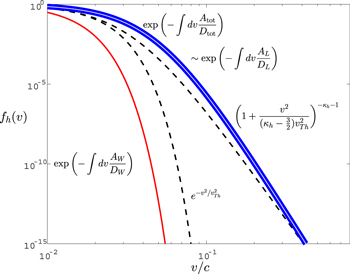
Figure 2. Revised halo VDF solution is shown with the thick blue curve. The initial guess, the kappa VDF defined in Equation (3), is depicted with dashes. The solution (21) in which the coefficients  and
and  are computed by ignoring the whistler contribution (only Langmuir fluctuation, AL and DL) are shown with the thin white curve and superposed on top of the total solution. As one can see, the total solution and the solution with only the Langmuir fluctuation are virtually identical. If, on the other hand, we ignore the L mode contribution but retain only the whistler (W) contribution, as was done in Kim et al. (2015) and Yoon et al. (2015), then we have the solution shown with the red curve. For comparison we plot the Gaussian VDF in dashes.
Download figure:
Standard image High-resolution imageIn the original model proposed by Kim et al. (2015) and Yoon et al. (2015) the halo VDF was constructed on the basis of the whistler fluctuation only. Such a model is equivalent to the approximation that in Equation (22) the coefficients  and
and  are evaluated by retaining only those terms containing the factor 1/r, while arbitrarily ignoring those terms without such a factor. In Figure 2 we denote such a solution by
and plot the result with the red curve. As one can see, such an approximate solution greatly deviates from the total solution shown in the thick blue line.
Finally, we plot the reduced solution in which the coefficients  and
and  in Equation (22) are approximately evaluated by ignoring terms associated with the 1/r factors. This is the solution constructed on the basis of Langmuir fluctuation and Landau resonance only, and is denoted by
The result is plotted with the thin white line, which is superposed on top of the thick blue line. As one can see, the two solutions are virtually identical, which proves that the Langmuir fluctuations are totally dominant, at least for the present choice of parameters including r = ωpe/Ωe = 50. However, it should also be noted that the kappa VDF assumed as an initial guess is NOT identical to the numerically obtained steady-state solution (first iteration), although it is not too far from being a solution.
We could, in principle, iterate the numerical procedure as many steps as desired, but in the present paper we only show the solution corresponding to one iteration, that is, assuming an initial kappa VDF (24), constructing the wave fluctuation spectrum (22), and inserting the result to the formal steady-state VDF (23), thereby obtaining the correction to the initial VDF. We have not rigorously checked the convergence of the iteration procedure. Alternatively, one could start from the time-dependent quasilinear particle and kinetic equation, and numerically solve the system until a quasi-saturation stage is achieved. We have not carried out such a task either.
Since we now know that Langmuir fluctuations totally dominate the solar wind electron VDF, the question is whether whistler fluctuations have an influence on the halo electrons at all under any circumstances. Recall that previous theoretical works emphasized the role of whistler turbulence in the halo and strahl electron dynamics (Vocks et al. 2005; Gary & Saito 2007; Saito & Gary 2007a, 2007b; Pierrard et al. 2011). Does our finding mean that all these works are irrelevant as well? The answer is not necessarily so. Note that the above-cited references pertain to dynamical situations where the whistler turbulence is presumed to be enhanced by some intrinsic processes, or is generated by instability. Under such scenarios the actual whistler intensity in the solar wind may be much higher than the level dictated by the spontaneous thermal emission theory. In fact, under some conditions, the whistler intensity level may be many orders of magnitude above the spontaneous emission level. To mimic such cases we arbitrarily multiply a scaling factor, S, to the whistler related terms (i.e., terms associated with 1/r factor) in the diffusion coefficient,  , in Equation (22)—but not in
  , since the enhanced whistler intensity does not affect the velocity space friction.
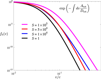
In Figure 3 we plot the unnormalized numerical solution (21) with the artificially enhanced whistler fluctuation intensity by multiplying the factor S to terms associated with 1/r terms in  . The figure is self-explanatory. The enhanced whistler wave intensity has no effect until S is raised as high as S = 104. Once S exceeds this threshold, however, the whistler turbulence begins to have an impact. This shows that enhanced whistlers, such as those excited by instability, or those that are intrinsic, such as remnants of a cascading solar wind turbulence, may after all lead to a substantial heating of the halo electrons. We caution the readers that the purpose of Figure 3 is not to address the self-consistent solution (i.e., coupled particle and wave equation), but rather to point out that whistler waves can be important under some circumstances. An artificially raised whistler fluctuation spectrum is not a steady-state solution of the wave kinetic equation.
Figure 3. Revised halo electron VDF (21) with the enhancement factor, S, multiplied to terms within the diffusion coefficient,  , associated with 1/r factors. The red curve is the solution with S = 1. No appreciable change was observed until S is increased to 104, then suddenly the halo VDF exhibits an overall increase. Values of S corresponding to 104, 5 × 10⁴, and 1 × 10⁵ are plotted with blue, red, and magenta curves, in that order.
Download figure:
Standard image High-resolution image
3. CONCLUSIONS AND DISCUSSION
In a recent pair of papers, Kim et al. (2015) and Yoon et al. (2015) suggested a model of the solar wind electrons during quiet time conditions. They separately considered the Gaussian core component, halo, and super-halo populations as making up the total electron VDF. In their model the Gaussian electrons remain non-resonant with any plasma collective oscillations, while the halo electrons were envisioned as having a steady-state interaction with the whistler-range fluctuations, where such fluctuations are self-generated by the halo electrons themselves via spontaneous emission. Similarly, the super-halo electrons were modeled as being in a dynamical steady-state with the Langmuir fluctuations, also self-generated by the super-halo electrons via a spontaneous thermal process. A subsequent paper by Kim et al. (2016), a third in the series, showed that the halo electrons actually emit both whistlers and Langmuir fluctuations by a spontaneous process (Figure 1), while the super-halo electrons contribute mainly to Langmuir fluctuations. This implies that the original model for the halo electrons must be revised, since in that model the halo electrons are assumed to emit mostly whistlers.
The present paper revisits the halo modeling by including both the Langmuir and whistler waves in the distribution function construction (see Equations (21) and (22)). Figure 2 plots the resulting generalized model VDF. To our surprise, the total solution shows that the whistler contribution is rather minimal and that the net solution could as well have been constructed solely on the basis of Langmuir fluctuations only from the outset. The reason for the minimal contribution by the whistlers can be understood upon rewriting the velocity friction and diffusion coefficients in dimensionless form (Equations (21) and (22)). The terms that depict the whistler cyclotron wave–particle resonance with the halo electrons have overall multiplicative factors that are proportional to the inverse powers of r = ωpe/Ωe, but this ratio is on the order of 10 or even 102. As a consequence, the whistler cyclotron resonance effects become extremely insignificant. This shows that the spontaneously emitted Langmuir modes in the solar wind, known as the quasi thermal noise, are important not only for super-halo electrons (Yoon 2014) but also for halo population as well.
This conclusion notwithstanding, the role of whistler fluctuations on the dynamical processes, that is, time-dependent situations, can be important, especially when there exists free energy sources such as the temperature anisotropies and/or a net drift between the core and halo. In such cases, the whistler anisotropy instability or the heat flux instability might be excited so as to raise the whistler fluctuation levels by many orders of magnitude above that of the spontaneous emission. Under such a condition, enhanced whistler fluctuations can indeed have a finite (and sometimes significant) impact on the heating and acceleration of halo electrons, as Figure 3 shows.
An important question that the present paper, or for that matter, earlier papers (Kim et al. 2015; Yoon et al. 2015) did not address is the question of the uniqueness of the kappa-like VDF for halo and super-halo. In Yoon (2014), this question was actually addressed for a single component electron VDF immersed in a self-generated field of Langmuir fluctuation in unmagnetized plasma. According to Yoon (2014), kappa VDF is actually a unique solution that describes the so-called "turbulent" equilibrium between a single component electron population and an enhanced Langmuir turbulence. The key to the proof is the nonlinear term in the wave kinetic equation. Within the context of a quasilinear wave kinetic equation, any form of electron VDF and the associated Langmuir turbulence intensity is possible. However, with the nonlinear term in the wave kinetic equation it was shown that the kappa VDF is the one and only solution. A similar analysis must be done for the Maxwellian core plus suprathermal electron model, but such a task must be considered as a future project.
Before we close, the purpose of the present paper had been to revisit the halo electron model by including both the Langmuir and whistler fluctuations as well as Landau and cyclotron resonance factors. However, in the present paper we have still resorted to the somewhat artificial separation of super-halo and halo electrons into two populations. In reality, however, the total non-thermal electrons need not be artificially divided into two components, as the formal solution (9) can be applied over an entire range of non-thermal electron energies. The more general solar wind electron VDF modeling that treats the net non-thermal electrons as a single component is beyond the scope of the present paper, but it is a subject of a future paper.
P.H.Y. acknowledges NSF grant AGS1550566 to the University of Maryland, and the support by the BK21 plus program from the National Research Foundation of Korea to Kyung Hee University, Korea. He also acknowledges the Science Award Grant from the GFT Foundation to the University of Maryland. G.S.C. was supported by the Basic Science Research Program through the National Research Foundation of Korea (NRF) funded by the Ministry of Education (NRF-2013R1A1A2058937). Y.J.M. is supported by the NRF of Korea grant funded by the Korean Government (NRF-2013M1A3A3A02042232).