


Abstract
Far-infrared images and photometry are presented for 201 Luminous and Ultraluminous Infrared Galaxies [LIRGs: log  , ULIRGs: log
  ], in the Great Observatories All-Sky LIRG Survey (GOALS), based on observations with the Herschel Space Observatory Photodetector Array Camera and Spectrometer (PACS) and the Spectral and Photometric Imaging Receiver (SPIRE) instruments. The image atlas displays each GOALS target in the three PACS bands (70, 100, and 160 μm) and the three SPIRE bands (250, 350, and 500 μm), optimized to reveal structures at both high and low surface brightness levels, with images scaled to simplify comparison of structures in the same physical areas of ∼100 × 100 kpc2. Flux densities of companion galaxies in merging systems are provided where possible, depending on their angular separation and the spatial resolution in each passband, along with integrated system fluxes (sum of components). This data set constitutes the imaging and photometric component of the GOALS Herschel OT1 observing program, and is complementary to atlases presented for the Hubble Space Telescope, Spitzer Space Telescope, and Chandra X-ray Observatory. Collectively, these data will enable a wide range of detailed studies of active galactic nucleus and starburst activity within the most luminous infrared galaxies in the local universe.
Export citation and abstract BibTeX RIS
1. Introduction
The Great Observatories All-Sky LIRG Survey (GOALS, Armus et al. 2009) combines both imaging and spectroscopic data for the complete sample of 201 Luminous Infrared Galaxies (LIRGs: log  ) selected from the IRAS Revised Bright Galaxy Sample (RBGS, Sanders et al. 2003). The full RBGS contains 629 objects, representing a complete sample of extragalactic sources with IRAS 60 μm flux density,
  Jy, covering the entire sky above a Galactic latitude of
  . The median redshift of objects in the GOALS sample is
  , with a maximum redshift of
  . As the nearest and brightest 60 μm extragalactic objects, they represent a sample that is the most amenable for study at all wavelengths.
The primary objective of the GOALS multi-wavelength survey is to fully characterize the diversity of properties observed in a large, statistically significant sample of the nearest LIRGs. This allows us to probe the full range of phenomena such as normal star formation, starbursts, and active galactic nuclei (AGNs) that power the observed far-infrared (FIR) emission, as well as to better characterize the range of galaxy types (i.e., normal disks, major and minor interactions/mergers, etc.) that are associated with the LIRG phase. A secondary objective is to provide a data set that is ideally suited for comparison with LIRGs observed at high redshifts.
GOALS currently includes imaging and spectroscopy from the Spitzer, Hubble, GALEX, Chandra, XMM-Newton, and now Herschel space-borne observatories, along with complementary ground-based observations from ALMA, Keck, and other telescopes. The GOALS project is described in more detail at http://goals.ipac.caltech.edu/.
Due to limitations in angular resolution, wavelength coverage, and sensitivity of pre-Herschel (IRAS, ISO, Spitzer, AKARI) FIR data, the spatial distribution of FIR emission within the GOALS sources, as well as the total amount of gas and dust in these systems, are poorly determined. The Herschel data will allow us, for the first time, to directly probe the critical FIR and submillimeter wavelength regime of these infrared luminous systems, enabling us to accurately determine the bolometric luminosities, infrared surface brightnesses, star formation rates, and dust masses and temperatures on spatial scales of 2–5 kpc within the GOALS sample.
This paper presents imaging and photometry for all 201 LIRGs and LIRG systems in the IRAS RBGS that were observed during our GOALS Herschel OT1 program. A more complete description of the GOALS sample is given in Section 2. The data acquisition is described in Section 3, and data reduction procedures are discussed in Section 4. The image atlas is presented in Section 5, and photometric measurements are given in Section 6. Section 7 contains a discussion of basic results, including comparisons with prior measurements, and a summary is given in Section 8. A reference cosmology of  and
and  km s.−1 Mpc−1 is adopted; however, we also take into account local non-cosmological effects by using the three-attractor model of Mould et al. (2000).
2. The GOALS Sample
The IRAS RBGS contains 179 LIRGs (log  ) and 22 ultra-luminous infrared galaxies (ULIRGs: log
  ); these 201 total objects comprise the GOALS sample (Armus et al. 2009), a statistically complete flux-limited sample of infrared-luminous galaxies in the local universe. In addition to the Herschel observations reported here, the GOALS objects have been the subject of an intense multi-wavelength observing campaign, including VLA 20 cm (Condon et al. 1990, 1996), millimeter wave spectral line observations of CO(1 → 0) emission (Sanders et al. 1991), sub-millimeter imaging at 450 μm and 850 μm (Dunne et al. 2000), near-infrared images from 2MASS (Skrutskie et al. 2006), optical and K-band imaging (Ishida 2004), as well as space-based imaging from the Spitzer Space Telescope (IRAC and MIPS, J. M. Mazzarella et al. 2017, in preparation), Hubble Space Telescope (ACS, A. S. Evans et al. 2017, in preparation), GALEX (NUV and FUV, Howell et al. 2010), and the Chandra X-ray Observatory (ACIS, K. Iwasawa et al. 2011; K. Iwasawa et al. 2017, in preparation). Extensive spectroscopy data also exist on the GOALS sample in the optical (Kim et al. 1995), and with Spitzer IRS in the mid-infrared (Stierwalt et al. 2013). Herschel Photodetector Array Camera and Spectrometer (PACS) spectroscopy was obtained in Cycles 1 and 2, targeting the [C ii] 157.7 μm, [O i] 63.2 μm, and [O iii] 88 μm emission lines, as well as the OH 79 μm absorption feature for the entire sample, and the [N ii] 122 μm line in 122 GOALS galaxies (Díaz-Santos 2013, 2014; T. Díaz-Santos 2017, in preparation). In addition, Herschel SPIRE FTS spectroscopy were obtained to probe the CO spectral line energy distribution from
  up to
up to  for 93 of the GOALS objects (Lu et al. 2014, 2015; N. Lu et al. 2017, in preparation), as well as the [N ii] 205 μm emission line for 122 objects Zhao et al. (2013, 2016).
Out of the original list of 203 GOALS systems, two were omitted from our Herschel sample, making for a final tally of 201 objects. IRAS F13097–1531 (NGC 5010) was part of the original RBGS sample of Sanders et al. (2003). However, due to a revision in the redshift of the object, it was much revealed to be closer than previously thought. This caused the resulting IR luminosity to drop significantly below the LIRG threshold of  . The other object we excluded from our sample is IRAS 05223+1908, which we believe is a young stellar object, due to the fact that its spectral energy distribution (SED) peaks in the submillimeter part of the spectrum.
Table 1 presents the basic GOALS information. Column 1 is the index number of galaxies in the GOALS sample, which correspond to the same galaxies in Tables 2–4. Column 2 is the IRAS name of the galaxy, ordered by ascending R.A. Note that galaxies with the "F" prefix originate from the IRAS Faint Source Catalog, and galaxies with no "F" prefix are from the Point Source Catalog. Column 3 is a list of common optical counterpart names. Columns 4 and 5 are the Spitzer 8 μm centers of the system in J2000 from J. M. Mazzarella et al. (2017, in preparation). For galaxy systems with two or more components, the coordinate is taken to be the geometric midpoint between the component galaxies. Column 6 gives the angular diameter distance to the galaxy in Mpc, from J. M. Mazzarella et al. (2017, in preparation). Column 7 is the map size used in the atlas, denoting the physical length of a side in each atlas image in kpc. Column 8 is the systemic heliocentric redshift of the galaxy system, and Column 9 is the measured heliocentric radial velocity in km sec−1, which corresponds to the redshift. Both of these columns take into account cosmological as well as non-cosmological effects (see Mould et al. 2000). Finally, Column 10 is the indicative 8–1000 μm infrared luminosity in log  of the entire system, from Armus et al. (2009). Similar to Columns 8 and 9, the LIR values in Table 1 take into account the effect of the local attractors to DA than one would normally obtain from pure cosmological effects.
Table 1. Basic GOALS Data
| # | IRAS Name | Optical Name | R.A. | Decl. | DA | Map Size | Redshift | Velocity |

|
|---|---|---|---|---|---|---|---|---|---|

|

|
Mpc | kpc | km s−1 | log 
|
||||
| (1) | (2) | (3) | (4) | (5) | (6) | (7) | (8) | (9) | (10) |
| 1 | F00073+2538 | NGC 23 | 00:09:53.36 | +25:55:27.7 | 63.3 | 100 | 0.01523 | 4566 | 11.12 |
| 2 | F00085-1223 | NGC 34, Mrk 938 | 00:11:06.56 | −12:06:28.2 | 81.5 | 100 | 0.01962 | 5881 | 11.49 |
| 3 | F00163-1039 | Arp 256, MCG-02-01-051/2 | 00:18:50.37 | −10:22:05.3 | 111.4 | 150 | 0.02722 | 8159 | 11.48 |
| 4 | F00344-3349 | ESO 350-IG 038, Haro 11 | 00:36:52.49 | −33:33:17.2 | 85.4 | 100 | 0.0206 | 6175 | 11.28 |
| 5 | F00402-2349 | NGC 232 | 00:42:49.32 | −23:33:04.3 | 91.3 | 150 | 0.02217 | 6647 | 11.44 |
| 6 | F00506+7248 | MCG+12-02-001 | 00:54:03.88 | +73:05:05.9 | 67.7 | 100 | 0.0157 | 4706 | 11.50 |
| 7 | F00548+4331 | NGC 317B | 00:57:39.72 | +43:47:47.7 | 74.1 | 100 | 0.01811 | 5429 | 11.19 |
| 8 | F01053-1746 | IC 1623, Arp 236 | 01:07:47.54 | −17:30:25.6 | 82.2 | 100 | 0.02007 | 6016 | 11.71 |
| 9 | F01076-1707 | MCG-03-04-014 | 01:10:08.93 | −16:51:09.9 | 134.8 | 100 | 0.03349 | 10040 | 11.65 |
| 10 | F01159-4443 | ESO 244-G012 | 01:18:08.27 | −44:27:51.9 | 87.7 | 100 | 0.02104 | 6307 | 11.38 |
Note. The column descriptions are (1) The row reference number. (2) The IRAS name of the galaxy, ordered by ascending R.A. Here, galaxies with the "F" prefix originate from the IRAS Faint Source Catalog, and galaxies with no "F" prefix are from the Point Source Catalog. (3) Common optical counterpart names to the galaxy systems. (4)–(5) are the Spitzer 8 μm centers of the system in J2000 (see J. M. Mazzarella et al. 2017, in preparation). The Herschel atlas images are centered on these coordinates. For widely separated systems, the coordinate is taken to be halfway between the component galaxies. (6) The angular diameter distance to the galaxy in Mpc, from J. M. Mazzarella et al. (2017, in preparation). (7) The map size used in the atlas, denoting the physical length of a side in each atlas image, in kpc. (8) The non-relativistic redshifts as reported by NED, which also corresponds to the heliocentric velocity (Column 9) and includes both cosmological and non-cosmological effects. (9) The measured heliocentric radial velocity, corresponding to the redshift in Column 8 in km s−1 from Armus et al. (2009), including both cosmological and non-cosmological effects. (10) The indicative infrared luminosity, measured in log  of the entire system, from Armus et al. (2009). These values take into account the effect of the local attractor to the distances that one would normally obtain from pure cosmological effects.
Only a portion of this table is shown here to demonstrate its form and content. A machine-readable version of the full table is available.
Download table as: DataTypeset image
Table 2. Herschel Observation Log
| PACS | SPIRE | |||||||||||||
|---|---|---|---|---|---|---|---|---|---|---|---|---|---|---|
| # | IRAS Name | Optical Name | Blue 1 | Blue 2 | Green 1 | Green 2 | Duration | Blue | Green | PACS | Obs. ID | Duration | Obs. Date | SPIRE |
| Obs. ID | Obs. ID | Obs. ID | Obs. ID | (s) | Obs. Date | Obs. Date | PIDa | (s) | PIDa | |||||
| (1) | (2) | (3) | (4) | (5) | (6) | (7) | (8) | (9) | (10) | (11) | (12) | (13) | (14) | (15) |
| 1 | F00073+2538 | NGC 23 | 1342225471 | 1342225472 | 1342225469 | 1342225470 | 198 | 2011 Jul 24 | 2011 Jul 24 | 1 | 1342234681 | 169 | 2011 Dec 18 | 1 |
| 2 | F00085-1223 | NGC 34, Mrk 938 | 1342212463 | 1342212464 | 1342212465 | 1342212466 | 276 | 2011 Jan 10 | 2011 Jan 10 | 3 | 1342199384 | 445 | 2010 Jun 29 | 3 |
| 3 | F00163-1039 | Arp 256, MCG-02-01-051/2 | 1342212700 | 1342212701 | 1342212702 | 1342212703 | 485 | 2011 Jan 15 | 2011 Jan 15 | 2 | 1342234694 | 169 | 2011 Dec 18 | 1 |
| 4 | F00344-3349 | ESO 350-IG 038, Haro 11 | 1342210636 | 1342210637 | 1342197713 | 1342197714 | 65c | 2010 Dec 01 | 2010 Jun 04 | 10 | 1342199386 | 307 | 2010 Jun 29 | 10 |
| 5 | F00402-2349 | NGC 232 | 1342238073 | 1342238074 | 1342237438 | 1342237439 | 240 | 2012 Jan 21 | 2012 Jan 13 | 1 | 1342234699 | 1217 | 2011 Dec 18 | 1 |
| 6 | F00506+7248 | MCG+12-02-001 | 1342237174 | 1342237175 | 1342237172 | 1342237173 | 198 | 2012 Jan 11 | 2012 Jan 11 | 1 | 1342199365 | 169 | 2010 Jun 29 | 4 |
| 7 | F00548+4331 | NGC 317B | 1342213944 | 1342213945 | 1342213946 | 1342213947 | 347 | 2011 Feb 08 | 2011 Feb 08 | 2 | 1342238255 | 169 | 2012 Jan 27 | 1 |
| 8 | F01053-1746 | IC 1623, Arp 236 | 1342212754 | 1342212755 | 1342212846 | 1342212847 | 65 | 2011 Jan 16 | 2011 Jan 18 | 2 | 1342199388 | 169 | 2010 Jun 29 | 2 |
| 9 | F01076-1707 | MCG-03-04-014 | 1342225341 | 1342225342 | 1342225343 | 1342225344 | 198 | 2011 Jul 23 | 2011 Jul 23 | 1 | 1342234709 | 169 | 2011 Dec 18 | 1 |
| 10 | F01159-4443 | ESO 244-G012 | 1342225365 | 1342225366 | 1342225363 | 1342225364 | 198 | 2011 Jul 23 | 2011 Jul 23 | 1 | 1342234726 | 169 | 2011 Dec 18 | 1 |
Notes. The column descriptions are (1) the row reference number. (2) The IRAS name of the galaxy, ordered by ascending R.A. The galaxies with prefix "F" originate from the IRAS Faint Source Catalog, and the galaxies with no "F" prefix are from the Point Source Catalog. (3) Common optical counterpart names to the galaxy systems. (4)–(7) are the observation IDs for PACS imaging. Blue corresponds to a wavelength of 70 μm, whereas green corresponds to 100 μm. Each blue and green observation simultaneously observes the red 160 μm channel. Each observation needs a separate scan and cross-scan to reduce imaging artifacts. Four galaxies in our sample do not have 100 μm observations available because they were taken from other programs: IRAS F02401-0013 (NGC 1068), IRAS F09320+6134 (UGC 05101), IRAS F15327+2340 (Arp 220), and IRAS F21453-3511 (NGC 7130). (8) The PACS observation duration for each scan and cross-scan, unless otherwise noted. We note these are not exposure times. (9)–(10) The observation dates for each scan and cross-scan, unless otherwise noted. (11) The PI of the PACS program from which the data were obtained. See PI list below. (12) The SPIRE observation ID, which includes all three 250, 350, and 500 μm observations. The scans and cross-scans for each target is combined into one observation. (13) The SPIRE observation duration. We note these are not exposure times. (14) The SPIRE observation date. (15) The PID of the SPIRE program from which the data were obtained. See PID list below.
aPI list: 1 = OT1_sanders_1; 2 = KPGT_esturm_1; 3 = GT1_msanchez_2; 4 = KPOT_pvanderw_1; 5 = KPOT_rkennicu_1; 6 = OT1_dfarrah_1; 7 = GT1_lspinogl_2; 8 = cwilso01_1 (including KPGT); 9 = OT1_mcluver_2; 10 = KPGT_smadde01_1. bThese are very widely separated galaxy pairs that required two Herschel PACS observations. cGreen 1 and Green 2 have durations of 65 s, Blue 1 has a duration of 141 s and Blue 2 has a duration of 153 s. dGreen 2 was observed on 2012 Apr 24. eGreen 2 was observed on 2012 Mar 29. fRescheduled to replace previous PACS observations: 1342245766 1342245767 1342245764 1342245765.Only a portion of this table is shown here to demonstrate its form and content. A machine-readable version of the full table is available.
Download table as: DataTypeset image
3. Herschel Space Observatory Observations
The Herschel Space Observatory (Pilbratt et al. 2010) imaging observations of the GOALS sample took place between the dates of 2011 March and 2012 June, through our Cycle 1 open time observing program OT1_dsanders_1 (PI: D. Sanders, Program ID #1279). Under our proposal, a total of 169 galaxy systems were observed by the PACS (Poglitsch et al. 2010) instrument in imaging mode, with data from the remaining 32 galaxy systems from other guaranteed time (GT) or open time key programs (KPOT) obtained from the Herschel Science Archive (HSA). In addition, we observed 160 targets with the Spectral and Photometric Imaging Receiver (SPIRE, Griffin et al. 2010), with the remaining 41 targets from other GT and KPOT programs extracted from the HSA. In total, 84.9 hr of observations were completed under our specific GOALS program, with 61.6 hr for PACS and 23.3 hr for SPIRE.
Broad-band imaging were obtained in the three PACS bands at 70, 100, and 160 μm, and the three SPIRE bands at 250, 350, and 500 μm. The normalized filter transmission curves are shown in Figure 1. Each SPIRE band has two curves associated with the filter, corresponding to the point source responsivity (solid) and extended source responsivity (dashed). This is important because some of the objects in our sample are extended even at SPIRE wavelengths (i.e., the LIRG IRAS F03316–3618/NGC 1365).
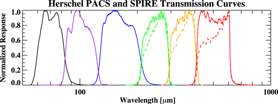
Figure 1. The normalized filter transmission curves for our Herschel data. From left to right are the PACS 70, 100, and 160 μm channels, followed by the SPIRE 250, 350, and 500 μm channels. For the SPIRE bands, the point source response is shown with a solid curve, and the extended source response is shown with a dashed curve. Note the large difference in response for the SPIRE 500 μm transmission curve.
Download figure:
Standard image High-resolution imageWithin the GOALS sample, there are eight systems consisting of widely separated pairs where two separate PACS observations were needed, but only one SPIRE observation was made because its field of view was larger. These galaxies are denoted in both Tables 1 and 2, giving a total of  observation data sets. We note that, for the galaxy system IRAS F07256+3355, which has three components, only two are visible in the PACS imagery due to its smaller field of view. The third component (NGC 2385) is far to the west, but still within SPIRE's larger field of view. Using the SPIRE fluxes as a rough proxy for infrared luminosity strength, NGC 2385 contributes very little to the overall infrared luminosity of the system. IRAS F23488+1949 also has a third component (NGC 7769) to the NNW in the SPIRE images, but is outside of the PACS scan area. However, from the SPIRE fluxes, NGC 7769 appears to have a moderate contribution to the system's infrared luminosity. In sum, we achieved a very high degree of coverage and completeness for each GOALS object with Herschel.
3.1. Photoconductor Array Camera and Spectrometer (PACS) Observations
The Photoconductor Array Camera and Spectrometer (PACS, Poglitsch et al. 2010) is one of three FIR instruments onboard the Herschel Space Observatory and covers a wavelength range between 60 and 210 μm. In the photometer mode, it can image two simultaneous wavelength bands centered at 160 μm, and at either 70 μm or 100 μm. These three broad bands are referred to as the blue channel (60–85 μm), green channel (85–130 μm) and red channel (130–210 μm). For any given observation, the blue camera observes at either 70 μm or 100 μm, whereas the red camera only observes at 160 μm. A dichroic beam-splitter with a designed transition wavelength of 130 μm directs the incoming light into the blue and red cameras, and a filter in front of the blue camera selects either the blue or green band.
The detectors for both the blue and red cameras comprise a filled bolometer array of square pixels that instantaneously samples the entire beam from the telescope's optics. The layout of the blue camera's focal plane consists of 4 × 2 subarrays, with 16 × 16 pixels in each subarray. Similarly, the red camera consists of 2 × 1 subarrays with 16 × 16 pixels each. On the sky, each bolometer pixel subtends an angle of 3 2 × 32 and 64 × 64 for the blue and red cameras, respectively. There exists gaps between each of the subarrays in both cameras, which must be filled in by on-sky mapping techniques (i.e., scan mapping). Both the blue and red cameras were designed to image the same 3
 5 × 175 field of view on the sky at any given instant.
In the photometer mode, there are two astronomical observing templates available, in addition to a PACS/SPIRE parallel observing mode. For our Herschel GOALS program, we used the scan map technique for all of our astronomical observing requests (AOR), which is ideal for mapping large areas of the sky and/or targets where extended flux may be present. Our scan map observations involve slewing the telescope at constant speed along parallel lines separated by 15'' from each other, perpendicular to the scan direction. Two example PACS observation footprints are shown in Figure 2 panels (a) and (c), overlaid on images from the Digital Sky Survey (DSS). The area of maximum coverage is the inner region centered on the red box, where the requested observation is centered. For the GOALS observations, we chose to observe seven scan legs in each scan and cross-scan using the 20'' s−1 scan speed, with scan leg lengths ranging between 3 and 6' depending on the size of the target. At this scan speed, the beam profiles for each wavelength have mean FWHM values of 56, 68, and 113 for the 70, 100, and 160 μm channels, respectively.

Figure 2. The PACS and SPIRE observation footprints for two galaxies, IRAS F18145+2205 (CGCG 142-034) in the top row, and IRAS F20221-2458 (NGC 6907) on the bottom. These figures were generated using HSPOT, the Herschel observation planning tool, whereas the background images used are from DSS. The red box in each panel indicates the central coordinate for each observation. The PACS observations are shown in panels (a) and (c), which display a 9' × 9' field of view around the target coordinate. Each scan leg in one direction is repeated several (nominally seven) times for maximal coverage of the source galaxy (or galaxies). The SPIRE observations are shown in panels (b) and (d), and have a 25' × 25' field of view, which is much larger than the PACS field of view. Panel (b) shows a small map scan, whereas the bottom panel shows a large map scan.
Download figure:
Standard image High-resolution imageBefore each PACS photometer observation is a 30 s chopped calibration measurement between two internal calibration sources (the calibration block), followed by 5 s of idle for telescope stability before the science observation is executed. As the telescope is scanned across the sky during science observations, all of the bolometer pixels are read out at a frequency of 40 Hz, even during periods where the telescope was turning around for the next scan leg. However, due to satellite data-rate limitations, all PACS data are averaged over four frames—effectively downsampling the data to 10 Hz. The result is a data timeline of the flux seen by each detector pixel as a function of time (and by extension, position on the sky) as the telescope is scanned over the target field.
In order to accurately reconstruct the image, two scan map AORs at orthogonal angles are required. This is because, as the telescope scans a field, the offsets of each bolometer subarray, and even each pixel, may be different from their neighbors, resulting in stripes or gradients in the final reconstructed map. However, if the same field is scanned in two orthogonal directions, many of these map artifacts can be successfully removed, by virtue of multiple different bolometers sampling each patch of the sky. Furthermore, in order to maximally sample a given sky pixel by as many bolometer pixels as possible, we chose our scan angles to be  and
and  , with respect to the detector array. The orthogonal scans similarly help remove drifts in the bolometer timelines. These time-dependent variations in the detector or subarray offsets can be caused by, for example, cosmic ray hits and other instrument effects. For our survey, the typical PACS scan duration is about 200 s. However, larger maps with deeper coverage can be as long as ∼1900 s. Because two scans are needed for each target in the blue and green filter, there are two pairs of scans and cross-scans in the red channel, giving us better sensitivity. Unfortunately, due to unforeseen consequences, several galaxy components in IRAS F02071–1023 and IRAS F07256+3355 had sufficient coverage from only one of the scans, which resulted in more noise along the scan direction around the target.
Because, by definition, all of the objects in the GOALS sample have an IRAS 60 μm flux of at least 5.24 Jy, the galaxies or galaxy systems are bright enough that only one repetition was needed for each PACS scan and cross-scan. With one pair of scan and cross-scan observations, we achieved a 1-σ point source sensitivity of approximately 4 mJy in the central area, and approximately 8 mJy averaged over the entire map for both blue and green observations. By combining all four red channel scans and cross-scans, we achieved a 1-σ point source sensitivity of about 6 mJy in the central area, and about 12 mJy averaged over the entire map. On the other hand, the extended flux sensitivities for one repetition (one scan and cross-scan pair) are 5.3 MJy sr−1, 5.2 MJy sr−1, and 1.7 MJy sr−1 for the 70 μm, 100 μm, and 160 μm channels, respectively.
3.2. SPIRE Observations
SPIRE (Griffin et al. 2010) is a submillimeter camera on Herschel that operates between the 194 and 671 μm wavelength range. In the imaging mode, it can simultaneously observe in three different broad bandpasses ( ), centered at 250, 350, and 500 μm. Similar to PACS, SPIRE images a field by scan mapping, where the instrument field of view (4' × 8') is scanned across the sky to maximize the spatial coverage. The three detector arrays use hexagonal feedhorn-coupled bolometers, with 139, 88, and 43 bolometers for the PSW (250 μm), PMW (350 μm), and PLW (500 μm) channels, respectively. The beam profiles for each wavelength have mean FWHM values of 181, 252, and 366 for the 250, 350, and 500 μm photometer arrays, and mean ellipticities of 7%, 12%, and 9% (the beam shape changes slightly as a function of off-axis angle).
There are three main observing modes available: point source photometry, field/jiggle mapping, and scan mapping. For our observing program (dsanders_OT1_1) we chose the scan-map mode at a scan rate of 30'' s−1, because it gave the best data quality as well as a larger field of view for the final map than the other two mapping modes. Nominal scan angles of 42 4 and 1272, with respect to the detector arrays, were used to maximize sky coverage by as many detectors as possible, as well as to minimize the effect of individual bolometer drift during data processing. Like PACS, two scans are needed for data redundancy as well as cross-linking; however, the scan and cross-scan with SPIRE are observed within a single AOR. Within our program, the vast majority of our targets were observed in the small map mode (∼150 targets), whereas the rest were taken in the large map mode (∼20 targets). The typical scan durations are ∼170 s. for small maps (∼5' × 5' guaranteed map coverage area), and up to ∼2200 s for large maps. In Figure 2 panels (b) and (d), we show two example observations using SPIRE. The top panel shows a small map mode observation, whereas the bottom panel shows a large map mode observation. In both cases, the SPIRE detector is scanned over the target coordinate (shown by the red box) from the top left to the bottom right, and then from the top right to the bottom left.
Due to the extremely sensitive design of the Herschel optics and SPIRE instrument, only one repetition was observed for every target in our observing program. The SPIRE instrument has a confusion limit of 5.8, 6.3, and 6.8 mJy beam−1 for the 250, 350, and 500 μm channels, which is defined as the standard deviation of the flux density in the limit of zero instrument noise (Nguyen et al. 2010). On the other hand, the instrument noise is about 9, 7.5, and 10.8 mJy beam−1 at 250, 350, and 500 μm for one repetition (scan and cross-scan) at the nominal scan speed of 30'' s−1. Because many of our targets have extended features, SPIRE's 1-σ sensitivities to extended flux are at the 1.4 MJy sr−1, 0.8 MJy sr−1, and 0.5 MJy sr−1 levels for 250, 350, and 500 μm for one repetition. These flux levels are already dominated by confusion noise, and more than sufficient to detect any cold dust components in our sample.
3.3. Observing Log
Table 2 below lists the observing log for our data sample. Column 1 is the galaxy reference number, and column 2 is the IRAS name of the galaxy, ordered by ascending R.A. Column 3 is the common optical counterpart names to the galaxy systems. Columns 4–7 are the observation IDs for PACS imaging. Blue corresponds to a wavelength of 70 μm, whereas green corresponds to 100 μm. Each blue and green observation pair simultaneously observes the red 160 μm channel. Two orthogonal observations are made at each wavelength to reduce imaging artifacts. We note that four galaxies in our sample do not have 100 μm observations available because they were taken from other programs that did not observe them: IRAS F02401-0013 (NGC 1068), IRAS F09320+6134 (UGC 05101), IRAS F15327+2340 (Arp 220), and IRAS F21453-3511 (NGC 7130). Column 8 is the PACS observation duration for each scan and cross-scan, unless otherwise noted. We note these are not exposure times, but instead the amount of time for each scan and cross-scan. Columns 9–10 are the observation dates for each pair of PACS scan and cross-scan, unless otherwise noted. Column 11 is the Program ID of the PACS program from which the data were obtained. We list the PID corresponding to each number in Table 2's caption. The bulk of the data (∼80%) are from OT1_sanders_1, with most of the remaining data from KPGT_esturm and KPOT_pvanderw_1. Column 12 is the SPIRE observation ID, which includes all three 250, 350, and 500 μm observations. The scans and cross-scans for each target are combined into one observation. Column 13 is the SPIRE observation duration, which is similar to the PACS duration. Column 14 is the SPIRE observation date, and column 15 is the PID of the SPIRE program from which the data were obtained, similar to the PACS PID column.
4. Data Processing and Reduction
The data processing for our Herschel data was performed using the Herschel Interactive Processing Environment (HIPE, Ott 2010) version 14 software tool, which provides the means to download, reduce, and analyze our data. All of our data reduction routines are derived from the standard pipeline scripts found within HIPE, where the programming language of choice is Jython (a Java implementation of the popular Python language). In addition to handling the data processing, HIPE also downloads and maintains all of the instrument calibration files needed for the data processing.
4.1. PACS Data Reduction
4.1.1. Choosing a PACS Map Maker
Due to the bolometer and scanning nature of the PACS instrument, it was important to determine the best map-making software to translate the time-ordered data (TOD) into an image. The PACS bolometers (indeed, all bolometers) produce noise that increases as one approaches lower temporal frequencies, commonly referred to as  noise, which must be removed by the map-maker. If this noise is left uncorrected in the TOD, the result would be severe striping or even gradients across the image. In addition, the map-making software must also remove the bolometers' common mode drift (which is a changing offset as function of time) from the TOD, termed pre-processing, as well as cosmic ray hits and individual bolometer drift. The PACS team released their Map-making Tool Analysis and Benchmarking report14
in 2013 November, with an update in March 2014 that characterized in detail the six different map making packages available to reduce PACS data. We summarize the information presented in this report below. They were used to decide upon the best map-making software to use, because it was important that all of the Herschel data on our sample were processed uniformly.
noise, which must be removed by the map-maker. If this noise is left uncorrected in the TOD, the result would be severe striping or even gradients across the image. In addition, the map-making software must also remove the bolometers' common mode drift (which is a changing offset as function of time) from the TOD, termed pre-processing, as well as cosmic ray hits and individual bolometer drift. The PACS team released their Map-making Tool Analysis and Benchmarking report14
in 2013 November, with an update in March 2014 that characterized in detail the six different map making packages available to reduce PACS data. We summarize the information presented in this report below. They were used to decide upon the best map-making software to use, because it was important that all of the Herschel data on our sample were processed uniformly.
The PACS team tested the performance of six different publicly available map-making packages: MADMap (Microwave Anisotropy Data set Mapper, Cantalupo et al. 2010), SANEPIC (Signal And Noise Estimation Procedure Including Correlation, Patanchon et al. 2008), Scanamorphos (Roussel 2013), JScanam (Jython Scanamorphos15 ), Tamasis (Tools for Advanced Map-making, Analysis and SImulations of Submillimeter surveys, Barbey et al. 2011), and Unimap (Piazzo et al. 2015) (see Sections 2 and 4 of the Map-making Tool and Analysis Benchmarking report for a description of each code). We did not consider the PACS high pass filter (HPF) reduction software, because HPF maps are background-subtracted and will miss a significant amount of extended emission outside approximately one beam area. To evaluate each of the packages, a combination of simulated and real data from PACS were used. Except in a few cases, most of our fluxes are within the benchmarking report's "bright flux regime" of 0.3–50 Jy, whereas the "faint flux regime" is defined to be 0.001–0.1 Jy (see Figure 5). Below, we summarize the five tests performed on each map maker from the benchmarking report:
- (1)A power spectrum analysis that tests the map maker's ability to remove noise while preserving extended fluxes over large angular sizes on the map. This tests each code's performance in removing the
 noise from the PACS data, and consequently, how well gradients and stripes are removed from the maps.
 - (2)A difference matrix is computed for each map maker's output, which evaluates differences in fluxes for individual sky pixels over the entire image. For each pixel, is computed and plotted against Strue, and the resulting scatter, offset, and slope are evaluated.
- (3)Each map maker's performance in point source photometry is compared to fluxes measured from the HPF maps for both bright (0.3–50 Jy) and faint (0.001–0.1 Jy) cases. Because the HPF maps produced by HIPE are designed specifically for the case of point sources, they provide the most accurate reference point source fluxes.
- (4)Extended source photometry tests each map maker's ability to recover extended flux over large areas of the map. To assess this, each code's output is compared to IRAS data on M31 from the Improved Reprocessing of the IRAS Survey (IRIS, Miville-Deschênes and Lagache 2005).
- (5)The noise characteristics each map maker introduces into the final map are evaluated. This includes statistical tests on the pixel-to-pixel variance, as well as the shape of the overall distribution of fluxes in each map pixel. The noise patterns are also evaluated with regard to how isotropic the noise appears in the maps.


Considering the results of these extensive tests, it was difficult to select the best map maker for our PACS data. We rejected the High Pass Filter method outright because many of our galaxies are easily resolved at the PACS wavelengths, and would therefore have a significant amount of extended flux missed by the HPF pipeline. We decided against using SANEPIC because it significantly overestimated the true flux for both bright and faint point source photometry. We also ruled out using Tamasis because it has a tendency to introduce more pronounced noise along the scan directions. This left us with four remaining choices: JScanam, MADMap, Scanamorphos, and Unimap. We finally decided on using JScanam to reduce all of our PACS data, as it gave the best balance between photometric accuracy and map quality. Specifically, it reproduced a power spectrum closest to the original, had the flattest  versus Strue plot, and yielded the most accurate photometry for both point and extended sources in both channels.
For a small fraction of our maps where JScanam could not remove all of the image artifacts (usually gradients due to non-optimal baseline subtraction), we used Unimap to process the data, because it performed just as well as JScanam. Unlike JScanam, Unimap approaches map making differently, using the Generalized Least Square approach, which is also known as the Maximum Likelihood method if the noise has a Gaussian distribution. For a very few cases where even Unimap did not produce optimal results, we resorted to using MADMap. This map maker requires that the noise properties of the detectors are determined a priori, from which a noise filter can be generated to filter out the  noise. Finally, despite the fact that not all of the PACS maps were generated using the same map maker, we note that the resulting photometry from all three map makers are remarkably consistent, as shown in the benchmarking report (and addendum) from the PACS team, thus giving one the freedom to use the map maker that produces the best image quality.
4.1.2. PACS Map Making with JScanam
All of our Herschel-GOALS PACS data were reduced in HIPE 14 using the latest available PACS calibration version 72_0, released in 2015 December. In order to alleviate the processing time for all 211 objects, we started our data processing from the Level 1 products downloaded from the HSA. These Level 1 data products have the advantage of an improved reconstruction of the actual Herschel spacecraft pointing, which reduces distortions on the PSF due to jitter effects. Compared to previous maps from our data processing, the new maps have slight shifts of up to ∼15, and slightly smaller PSFs in unresolved GOALS objects.
Because each PACS scan and cross-scan are separate observations, JScanam requires two observations each for the blue and green data. On the other hand, the red channel data are observed simultaneously, regardless of whether the blue or green filter is used, so we have four observations in the red channel. Processing for both the blue and red cameras are identical, with the red data requiring a further step of combining the two pairs of scan and cross-scan data. Below, we describe the key steps in the data reduction process.
After loading each scan and cross-scan observation context from HSA into HIPE, the first step was to execute the task photAssignRaDec to assign the R.A. and decl. coordinates to each pixel in each frame, which allows JScanam to run faster. The next step was to remove the unnecessary frames taken during each turnaround in the scan or cross-scan, using the scanamorphosRemoveTurnarounds task. We opted to use the default speed limit, which is ±50% of our nominal scan speed (20'' s−1), so any frames taken at scan speeds below 10'' s−1 or above 30'' s−1 were removed. After turnaround removal, the scanamorphosMaskLongTermGlitches task in JScanam goes through the detector timelines and masks any long term glitches.
At this point, we have a detector timeline of flux detected by the bolometers as a function of time with the turnarounds and long term glitches removed. Using the scanamorphosScanlegBaselineFitPerPixel task, our next step is to subtract a linearly fit baseline from each bolometer pixel of every scan leg, with the intention of creating a "naive" map for source masking purposes. This is done iteratively, where the most important parameter is the nSigma variable, which controls the threshold limit for source removal. For our data, any points above nSigma = 2 times the standard deviation of the unmasked data are considered real sources, until the iteration converges.
The next step is to join the scan and cross-scan data together for a higher signal-to-noise map to create the source mask. In the scanamorphosCreateSourceMask task, we set nSgima = 4, so that any emission above four standard deviations is masked out. At this point, it is not necessary to mask out all of the faint extended emission, only the brightest regions. After the source mask is determined, they are applied to the individual scan and cross-scan timelines and the real processing begins.
With the galactic option set to "true" in scanamorphosBaselineSubtraction, we only want to remove an offset in the TOD over all the scan legs, and subtract it from all the frames. This is done by calculating a median offset over only the unmasked part of the data, which importantly does not include any bright emission, and subtracting it from each pixel's timeline. This is so that extended flux is treated correctly when subtracting the baseline (due to the telescope's own infrared emission) from the signal timelines, even in cases where the emission is not concentrated in a small region. We emphasize that this does not imply the subtraction of the Galactic foreground emission from our maps.
Once the baseline is removed, we need to identify and mask the signal drifts produced by the calibration block observation. In previous versions of our reduction, these drifts have produced very noticeable gradients in our final maps. To do this, the task scanamorphosBaselinePreprocessing assumes that the scan and cross-scan are orthogonal to each other, which would result in gradients in different directions. The drift removal is also based on the assumption that the drift power increases with the length of the considered time (1/f noise). For this reason, the first iteration removes the drift component over the longest timescale, which is the entire scan (or cross-scan). After that, drifts are removed over four scan legs, and finally over one scan leg, with the remaining drift in each successive iteration becoming weaker. In order to actually calculate the drift in each iteration, a single scan (or scan legs) is back-projected over itself in the orthogonal direction, which transforms the generally increasing or decreasing signal drift into oscillatory drifts that cancel out on large timescales. The orthogonal back-projected timeline is then subtracted from the scan timeline, and the difference, which represents the drift, is fitted by a line.
At this point, the scan and cross-scan data have been cleaned enough to be combined. Because signal drifts were only eliminated over timescales down to one scan leg, the next step is to remove them from over timescales shorter than one scan leg. These drifts are due to, for example, cosmic ray hits on the PACS instruments, which produce different effects on the TOD depending on which part is hit. If an individual bolometer or bolometer wall is hit, it only affects that bolometer. However, if a cosmic ray hits the readout electronics, it introduces a strong positive or negative signal for all of the bolometers read by the electronics, which can be anything from a single bolometer to an entire detector group. These jumps typically last a few tens of seconds before settling to the previous level again, and would result in stripes across the final map if not properly removed.
To remove these individual drifts, we use the task scanamorphosIndividualDrifts to first measure the scan speed and calculate the size of a map pixel that can hold six subsequent samples of a detector pixel crossing it. We use a threshold of nSigma = 5, which is large enough to include the strongest drifts but still mask out the real source. Next, the average flux value and standard deviation from the detector pixels crossing that map pixel are calculated, along with the number of detector pixels falling into that map pixel. Using the threshold noise value (from the calibration files), we eliminate any individual detector fluxes for that map pixel that have a standard deviation greater than the noise threshold. The missing values are then linearly interpolated, and the individual drift is subtracted from the detector timeline.
After all of the individual drifts are corrected, the TOD are saved and we project the timelines from both the scans and cross-scans into our final map, using the photProject task. We use a pixel scale of 16 pixel−1 for the 70 and 100 μm maps, and a pixel scale of 32 pixel−1 for the 160 μm maps. By default, the photProject task assumes, in projection, an active pixel size of 640 μm. However, if we "drizzle" the projection, we can assume smaller PACS pixels. This allows us to reduce the noise correlation between neighboring map pixels and also sharpens the PSF. We used a pixfrac of 0.1, which controls the ratio between the input detector and map pixel sizes. At this point, the 70 and 100 μm maps are finished. For the 160 μm data, both pairs of scan and cross-scan are identically processed separately, and then combined in the end, using photProject again.
4.2. SPIRE Data Reduction
4.2.1. Choosing a SPIRE Map Maker
Similar to the PACS instrument, the SPIRE detectors exhibit certain effects that are characteristic of bolometers. Namely, they introduce an increasing amount of noise as the length of the considered time increases ( noise), as well as constant and changing offsets (drifts) that could result in stripes or gradients in the final image. Therefore, any map maker for SPIRE must be able to remove these instrumental effects, but preserve flux (point source and extended) and create distortion-free maps. The SPIRE team released a Map Making Test Report16
in 2014 January that benchmarked in depth seven different map making codes, several of which were also present in the PACS Map Making report. The map makers that participated in the benchmarking were the Naive Mapper, Destriper in two flavors (P0 and P1), Scanamorphos, SANEPIC, and Unimap. The two flavors of the Destriper differ in the polynomial order used to subtract the baseline, where P0 corresponds to a polynomial order of 0 (i.e., the mean), and P1 corresponds to an order of 1. Two additional super-resolution map makers were also tested; however, we did not consider them for processing our SPIRE data. For a summary of each map maker, we refer the reader to the SPIRE Map Making Test Report.
noise), as well as constant and changing offsets (drifts) that could result in stripes or gradients in the final image. Therefore, any map maker for SPIRE must be able to remove these instrumental effects, but preserve flux (point source and extended) and create distortion-free maps. The SPIRE team released a Map Making Test Report16
in 2014 January that benchmarked in depth seven different map making codes, several of which were also present in the PACS Map Making report. The map makers that participated in the benchmarking were the Naive Mapper, Destriper in two flavors (P0 and P1), Scanamorphos, SANEPIC, and Unimap. The two flavors of the Destriper differ in the polynomial order used to subtract the baseline, where P0 corresponds to a polynomial order of 0 (i.e., the mean), and P1 corresponds to an order of 1. Two additional super-resolution map makers were also tested; however, we did not consider them for processing our SPIRE data. For a summary of each map maker, we refer the reader to the SPIRE Map Making Test Report.
For the Map Making Test Report, the authors tested these five map makers based on a variety of benchmarks that are very similar to the PACS Map-Making Tool Analysis and Benchmarking Report. A combination of real and simulated SPIRE data were used, covering the full variety of science cases, such as faint versus bright sources, extended versus point sources, and complex versus empty fields. The simulated SPIRE data have the advantage of comparing each of the map makers' outputs to the "truth" image, allowing for an unbiased comparison between all of the map making codes. These simulated observations were synthesized from two different layers: a truth layer based on a real or artificial source, and a noise layer from real SPIRE observations, so that both instrumental and confusion noise is accurately represented. Below, we summarize the four metrics and performance results for the five possible map makers:
- (1)Using simulated data, the deviation of each map maker's output is compared to the original synthetic data. To quantify the deviation from truth, a scatter plot of is plotted against Strue, and the resulting slopes, relative deviations, and absolute deviations are compared.
- (2)The 2D power spectrum of each map makers' output is compared to the "truth" image. The goal here is to quantify how well noise is removed from the maps while leaving real fluxes (point and extended) intact, as well as how high spatial frequency (small spatial scale) fluxes are treated.
- (3)Using the simulated data, point source photometry from each of the map makers were compared to the "truth" images. This tests how well point source fluxes are recovered by each map maker, in both the bright ( mJy) and faint ( mJy) regimes.
- (4)Finally, extended source photometry was tested between all the map makers using the synthetic data. A simulated exponential disk with an e-folding radius of 90'' was used, and fluxes were measured using aperture photometry.


Using the results from these tests, we concluded that the best map maker to use was the Destriper P0 mapper. It performed remarkably well among the other map makers, especially in cases where complex extended emission is present. Although the Map Making report warned about its inability to properly remove the "cooler burp" effect, the most recent version of Destriper P0 in HIPE 14 was updated to include proper treatment of this instrument effect. On the other hand, Destriper P1 compared unfavorably, especially in introducing artificial gradients in many cases. The Naive Mapper was also ruled out due to it frequently over-subtracting the background where extended emission is present. The map maker SANEPIC showed significant deviations from the "truth" map, because the code makes some incorrect assumptions about the data. Finally, although Scanamorphos can handle faint pixels very well, it showed significant deviations in the bright pixel case ( Jy). This is important because many galaxies in our sample are nearby, and thus quite bright.
In HIPE 14, we used a more advanced version of the Destriper code called the "SPIRE 2-Pass Pipeline" that was released by the SPIRE instrument team. The basic pipeline processing steps and settings follow exactly that of the Destriper P0 (or P1 if the user so chooses) map maker, with the added benefit of producing exceptionally clean maps to be used in the final Herschel Science Archive. Specifically, the 2-Pass Pipeline mitigates residual faint tails and glitches in the timeline, which can produce ringing effects if not removed. The primary aim of this pipeline is to produce maps with better detections of outliers in the TOD, such as glitches, glitch tails, and signal jumps, and remove any Fourier ringing that would result from failed outlier detections. As an overview, the first pass runs a stripped-down version of the pipeline, using only the bare minimum tasks, which exclude any Fourier Analysis. This first pass includes running the Deglitching task to produce a mask over the glitches, which is then applied back to the Level 0.5 products.17 A second pass of the pipeline is then executed, identical to the original Destriper map maker.
4.2.2. SPIRE Map Making With 2-pass Pipeline and Destriper P0
Our final SPIRE maps were reduced in HIPE 14, using the latest calibration version SPIRECAL_14_2 (released in 2015 December). Below, we summarize the key data reduction steps. However, a more detailed description of the photometer pipeline can be found within Dowell et al. (2010).
Our data processing begins with the Level 0 data products downloaded from HSA, which are the raw data formatted from satellite telemetry containing the readout in ADU from each SPIRE bolometer. After an observation is loaded into HIPE, the first step is to execute the Common Engineering Conversion and format it into Level 0.5 products. These products are the uncalibrated and uncorrected timelines measured in Volts, and contain all of the necessary information to build science-grade maps.
The first step in processing our data from Level 0.5 to Level 1 is to join all the scan legs and turnarounds together. The turnaround occurs when the spacecraft turns around after a scan leg to begin another scan. We opted to use the turnaround data to include as much data within our maps as possible. Next, the pipeline produces the pointing information for the observation, based on the positions of the SPIRE Beam Steering Mechanism as well as the offset between SPIRE and the spacecraft itself (referred to as the Herschel Pointing Product). This results in the SPIRE Pointing Product, which is used later on in the pipeline. After calculating the pointing information, the pipeline corrects for any electrical crosstalk between the thermistor-bolometer channels. The thermistors measure the temperature of the array bath as a function of time, so that later we may accurately subtract the instrument thermal contribution, or temperature drift from the data timelines.
The next step is the signal jump detector, which detects and removes jumps in the thermistor timelines that would otherwise cause an incorrect temperature drift correction. To do this, the module subtracts baselines and smoothed medians from the thermistor timelines to identify any jumps. After deglitching the thermistor timelines, we must deglitch any cosmic ray hits on the bolometers themselves. This is an important step, because any glitches that are not removed would manifest as image artifacts on the final maps. The pipeline does this in two steps, where the first step is to remove glitches that occur simultaneously in groups of connected bolometer detectors. This can occur when a cosmic ray hits the substrate of an entire photometer array, and can leave an imprint of the array on the final map. The second step is to run the wavelet deglitcher on the timeline data, which uses a complex algorithm to remove glitches in Fourier space.
After deglitching the detector timelines, a low pass filter response correction is applied to the TOD. This is to take into account the delay in the electronics with respect to the telescope position along a scan, in order to ensure a match between the astrometric timeline from the telescope and the detector timeline from the instrument. At this point, we can apply the flux conversion to the detector timelines, changing the units from Volts to Jy beam−1. The next step involves corrections to the timelines due to temperature drifts, which are caused by variations of the detector array bath temperatures. First, with the coolerBurpCorrection flag set to true, the pipeline flags data that were affected by the "cooler burp" effect. Observations taken during this effect, usually in the first ∼8 hr of SPIRE observations, can create unusual temperature drifts. The temperature drift correction step then removes low-frequency noise by subtracting a correction timeline for each detector, using data and calibration information. The "cooler burp" is also removed at this stage by applying additional multiplicative factors to the correction timeline.
Next, we apply a bolometer time-response correction that corrects any remaining low-level slow response from the bolometers. This is done by multiplying the timelines in Fourier space by an appropriate transfer function, obtained from a calibration file containing the detector time constants. After this step, we attach the R.A. and decl. to the data timelines by using the SPIRE Pointing Product generated earlier. Because many of our objects are extended in nature, we must apply an additional extended emission gain correction for individual SPIRE bolometers. This is because the pipeline assumes uniform beams across the array, whereas in reality there exist small variations among different bolometers, due to their positions on the array.
We then use the Destriper to remove striping from the final maps. Because the dominant fluxes seen by SPIRE are from the telescope itself, the science signal is very small in comparison. Therefore, to isolate the science signal, we must subtract out thermal contributions from the telescope. However, even after doing this, there are still large differences in residual offsets between different bolometers, due to variations in the thermal and electronic aspects of the system, resulting in striping. This is where the Destriper P0 comes in. It effectively takes SPIRE Level 1 context as input, and outputs destriped Level 1 timelines. To do this, we first subtract a median baseline as an initial guess, then we use a polynomial order of 0 to iteratively update the offsets in the TOD for each detector until an optimal solution is found. This algorithm effectively normalizes the map background to zero. However, we do include the true background using data from the Planck High Frequency Instrument (HFI) for the PMW and PLW arrays (see Section 6.2.1). After destriping, we run the optional second-level deglitching in order to remove any residual glitches that may still remain.
At this point, the data have been processed to Level 1, and in the case of the first pass, only tasks that do not involve any manipulation in Fourier space were omitted. The resulting second-level deglitching mask from the first pass of this pipeline is applied to the Level 0.5 data, and the entire process is repeated in a second pass, this time including operations in Fourier space.
The final step in our SPIRE data reduction is to project the drift-corrected, deglitched, and destriped timelines into our Level 2 science grade map. To do this, we use a Naive Mapper, which simply projects the full power seen by a bolometer onto the nearest map pixel. The final map pixel scales used were 6'', 10'', and 14'' for the PSW, PMW, and PLW arrays, respectively. For each instant of time on each bolometer's timeline, the measured flux is added to the total signal map, and a value of 1 is added to the coverage map. Once this is done for all bolometer timelines, the total signal map is divided by the coverage map to obtain the flux density map.
Although the 2-pass pipeline does an excellent job of removing all SPIRE image artifacts, approximately twenty of the maps still exhibited stripes and residual glitches in the final map. These maps were reprocessed by first using the SPIRE bolometer finder tool to identify the misbehaving bolometer, and then masking the affected portions in that bolometer's Level 1 timeline. The data were then rerun through the Naive Mapper to produce a clean and deglitched Level 2 science grade map.
5. The Herschel-GOALS Image Atlas
In the following pages, Figure 3 presents the entire Herschel atlas of the GOALS sample, ordered by ascending R.A. The archived18 Herschel GOALS maps are in standard ∗.fits format with image units of Jy pixel−1. Each page consists of six panels for the 70, 100, 160, 250, 350, and 500 μm channel maps.

Figure 3.
The Herschel GOAL Satlas, displaying imagery of local LIRGs and ULIRGs in the three PACS and three SPIRE bands. An asinh transfer function is used to maximize the dynamic range of visible structures, and a common field of view of approximately ∼100 × 100 kpc2 is used to facilitate comparisons across the sample and with images in the GOALS Spitzer atlas in J. M. Mazzarella et al. (2017, in preparation). Scale bars indicate 10 kpc and the equivalent angular scale as derived from the angular diameter distance in Table 1. The beam sizes at each wavelength are indicated on the lower right of each panel. The atlas is ordered by increasing right ascension. (The complete figure set of 209 atlas images is available.)
Download figure:
Standard image High-resolution imageThe IRAS name of each galaxy or galaxy system is shown at the top, along with their common names from optical catalogs. Each of the six panels are matched and have the exact same map center, as well as field of view. The center coordinates of the Herschel atlas images are listed in Table 1. For galaxy systems with multiple components, the center coordinate is chosen to be roughly equidistant from all components. The field of view for each panel is shown on the bottom left of the 70 μm panel, and represents the physical length of one side of each panel. A scale bar also indicates the physical length of 10 kpc at the distance of the galaxy (derived from the angular diameter distance in Table 1), along with the equivalent angular distance. The circle on the bottom right of each panel represents the beam size at that wavelength. Finally, the R.A. and decl. coordinates are indicated in J2000 sexagesimal, as well as decimal format. The sexagesimal R.A. coordinates have the hour portion truncated for all but the center tick mark, to keep the tick name sizes manageable.
Because many objects appear as point sources at some or all of the Herschel wavelengths, the morphologies of these galaxies will be dominated by the PSF at that wavelength. In the case of PACS, the PSF is characterized by a narrow circular core elongated in the spacecraft z-direction, at 70 and 100 μm. In addition, there is a tri-lobe pattern at the several percent level at all three wavelengths; however, it is strongest at 70 μm. Finally, there are knotty structured diffraction rings at the sub-percent level, again most apparent at 70 and 100 μm. In the case of SPIRE, the PSF appears mostly circular; however, for the brightest objects, airy rings are also visible.
In order to show as much detail as possible in these maps, we used an inverse hyperbolic sine (asinh) stretch function to maximize the dynamic range of visible structures. To keep all the PACS images uniform, the background for each image was also adjusted such that the background is very close to zero. The format in our Herschel atlas matches that of companion image atlases from Hubble Space Telescope-ACS (A. S. Evans et al. 2017, in preparation) and Spitzer-IRAC/MIPS (J. M. Mazzarella et al. 2017, in preparation), allowing one to study the morphological properties of these galaxies from 0.4 to 500 μm.
6. Herschel-GOALS Aperture Photometry
In this section, we discuss the manner in which the broadband photometry were determined for our sample. Both PACS and SPIRE photometry were obtained using the annularSkyAperturePhotometry routine found in HIPE. At first, we attempted to measure fluxes by using an automated routine to determine the appropriate circular aperture sizes for each galaxy, based on data from the MIPS instrument on Spitzer. Unfortunately, this approach does not work well for our sample, due to the extended nature of some GOALS systems and galaxies.
Instead, we concluded that the best approach was to determine apertures by visual inspection, and subsequently check that we included all of the flux by plotting a curve of growth. We found that, after subtracting any offset in the background levels, the curve of growth almost always flattens out at large radii, indicating a background flux contribution of zero. There are only a few small cases in the PACS data where the curve of growth does not flatten out, and in all cases this occurs when the object is very faint ( Jy) and the background noise is more dominant. Curve of growth plots for the SPIRE data are also flat at large radii, even for faint fluxes, again indicating robust background subtractions. In Figure 4, we show a set of representative curve-of-growth plots and apertures for IRAS F09111–1007 at different wavelengths. The photometry aperture is represented by the blue circle in the image and the blue line in the curve of growth plot below it. In order to facilitate comparison of matched aperture fluxes, all PACS aperture sizes are identical; all SPIRE apertures are also identical, but larger than those of PACS. The aperture radius is typically set by the band with the largest beam size for which we can make a measurement for each instrument; usually the 160 μm channel for PACS, and the 500 μm channel for SPIRE. We found that aperture radii encompassing approximately 95% of the total light gave the best tradeoff between including all of the flux and keeping the background error from getting too high. Although it is possible to use the same aperture size across all six bands (i.e., the SPIRE aperture size), the larger SPIRE aperture would encompass a significant amount of sky background for the higher-resolution images (i.e., at 70 μm), and would introduce additional noise in our measurements. We therefore decided it was best to match the apertures for each instrument.

Figure 4. Twelve curve-of-growth plots for IRAS F09111–1007, which are representative for the entire GOALS sample. The blue circle in each image is the photometry aperture, whereas the red circles are the annuli from which the background is measured. These circles are represented in the curve of growth plot immediately below each image. The first column shows the PACS 70, 100, and 160 μm photometry apertures for the western component of the system. The second column shows the PACS photometry apertures for the eastern nucleus. The third column shows the PACS photometry apertures encompassing both galaxies, which includes flux not in the component apertures, giving the total flux from this system. In the SPIRE bands, we only computed component fluxes at 250 μm because the galaxy pair is still resolved. However, because the galaxies are essentially unresolved in the other two SPIRE bands, we only compute total fluxes at those two wavelengths. Note that the fourth column only shows the total SPIRE apertures of both galaxies; the individual 250 μm plots were omitted to keep the figure manageable.
Download figure:
Standard image High-resolution imageTo accurately measure the flux of each galaxy, the sky background must be subtracted from the measured flux. To do this, we estimate the sky background in the annulus represented by the red circles in the image, which corresponds to the two red lines in the curve of growth plot. These background annuli were chosen to be as free from any source emission as possible. Within the annularSkyAperturePhotometry routine, we used the sky estimation algorithm from DAOPhot 19 to estimate the sky level, with the "fractional pixel" setting enabled. The background corrected flux density is then the total flux minus the product of the measured background level and the number of pixels within the target aperture.
We note that, in some cases, both component and total fluxes are measured for close pairs. These galaxies can be easily resolved and separated at shorter wavelengths, but become unresolved at longer wavelengths. In order to choose the best flux aperture, we carefully selected the radius at which the curve of growth was flattest. This is apparent in Figure 4, in the first two columns, where the galaxy pair is easily resolved at 70 μm but becomes marginally resolved at 160 μm. The third column in Figure 4 shows the curve of growth from a single large aperture encompassing the entire system, which includes faint extended flux missed by the individual component apertures. Finally, because the galaxy pair is unresolved in the 350 and 500 μm SPIRE bands, we do not measure any component fluxes at those wavelengths. At 250 μm, component fluxes are still computed because the pair is still resolved. Every effort was made to measure as many marginally resolved systems as possible, and also provide a total flux measurement from one large aperture when necessary. We believe separately measuring component and total fluxes in cases such as this will be useful when the fractional flux contribution of each component is desired.
In Table 3, we present the table of monochromatic total flux density for each GOALS system in units of Jansky. Depending on the number of galaxies within a system, their apparent separation on the sky, and the beam size at that particular wavelength, the total Herschel flux for each system is calculated using one of three methods. In the simple case of single galaxy, the system flux is just the flux of that galaxy. In cases where there are two or more galaxies that are widely separated, the total flux is the sum of the component fluxes measured in separate apertures. Finally, in cases where component galaxies are resolved but still overlapping (i.e., in Figure 4), the total system flux is obtained from a single large aperture encompassing all of the components. For triple and quadruple systems where two galaxies are close and a third (or fourth) is far away (i.e., IRAS F02071–1023), the total system flux is calculated using a hybrid method: a single large aperture for the two close components, plus a second (or third) aperture around the far component(s). Because all of the total fluxes are calculated differently, we omit the coordinate and aperture radius in Table 3, but we include it in Table 4 (see below).
Table 3. PACS and SPIRE Total Fluxes of GOALS Systems
| PACS | SPIRE | |||||||
|---|---|---|---|---|---|---|---|---|
| # | IRAS Name | Optical Name |

|

|

|

|

|

|
| (Jy) | (Jy) | (Jy) | (Jy) | (Jy) | (Jy) | |||
| (1) | (2) | (3) | (4) | (5) | (6) | (7) | (8) | (9) |
| 1 | F00073+2538 | NGC 23 | 10.48 ± 0.52 | 14.26 ± 0.71 | 11.85 ± 0.59 | 5.311 ± 0.347 | 2.026 ± 0.134 | 0.718 ± 0.046 |
| 2 | F00085-1223 | NGC 34, Mrk 938 | 18.21 ± 0.84 | 17.68 ± 0.81 | 10.65 ± 0.48 | 3.573 ± 0.214 | 1.239 ± 0.075 | 0.339 ± 0.021 |
| 3 | F00163-1039 | Arp 256, MCG-02-01-051/2 | 8.038 ± 0.403 | 9.876 ± 0.495 | 7.496 ± 0.375 | 2.862 ± 0.189 | 1.209 ± 0.081 | 0.419 ± 0.033 |
| 4 | F00344-3349 | ESO 350-IG 038, Haro 11 | 6.195 ± 0.276 | 5.096 ± 0.228 | 2.341 ± 0.101 | 0.639 ± 0.038 | 0.216 ± 0.014 | 0.067 ± 0.006 |
| 5 | F00402-2349 | NGC 232 | 14.60 ± 0.56 | 20.00 ± 0.77 | 16.11 ± 0.60 | 6.397 ± 0.323 | 2.441 ± 0.124 | 0.703 ± 0.035 |
| 6 | F00506+7248 | MCG+12-02-001 | 25.31 ± 1.27 | 29.07 ± 1.45 | 20.34 ± 1.02 | 7.968 ± 0.485 | 2.793 ± 0.174 | 0.896 ± 0.057 |
| 7 | F00548+4331 | NGC 317B | 10.91 ± 0.55 | 13.07 ± 0.65 | 9.945 ± 0.498 | 4.014 ± 0.266 | 1.600 ± 0.108 | 0.478 ± 0.039 |
| 8 | F01053-1746 | IC 1623, Arp 236 | 25.56 ± 1.28 | 29.28 ± 1.47 | 21.46 ± 1.08 | 8.991 ± 0.546 | 3.277 ± 0.201 | 1.023 ± 0.062 |
| 9 | F01076-1707 | MCG-03-04-014 | 8.996 ± 0.410 | 11.37 ± 0.51 | 8.758 ± 0.388 | 3.077 ± 0.187 | 1.181 ± 0.074 | 0.349 ± 0.023 |
| 10 | F01159-4443 | ESO 244-G012 | 9.934 ± 0.498 | 10.88 ± 0.54 | 7.735 ± 0.387 | 2.948 ± 0.194 | 1.155 ± 0.077 | 0.341 ± 0.025 |
Notes. The monochromatic flux density is given in units of Jansky for each of the three PACS and three SPIRE broadband filters. These are the total fluxes for each GOALS system. The column descriptions are (1) the row reference number. (2) The IRAS name of the galaxy, ordered by ascending R.A. Those galaxies with the "F" prefix originate from the IRAS Faint Source Catalog, and galaxies with no "F" prefix are from the Point Source Catalog. (3) Common optical counterpart names to the galaxy systems. Columns (4)–(6) are the fluxes from the PACS instrument in units of Jy. Note that the four galaxies that lack 100 μm measurements are IRAS F02401-0013 (NGC 1068), IRAS F09320+6134 (UGC 05101), IRAS F15327+2340 (Arp 220), and IRAS F21453-3511 (NGC 7130). Columns (7)–(9) are the fluxes from the SPIRE instrument in units of Jy.
aThese are very widely separated galaxy pairs that required two Herschel PACS observations. bThis is a triple system. However, only two component galaxies are visible in PACS due to its smaller field of view. The total flux for this system does not include the third galaxy not visible in PACS.Only a portion of this table is shown here to demonstrate its form and content. A machine-readable version of the full table is available.
Download table as: DataTypeset image
Table 4. PACS and SPIRE Total and Component Fluxes of GOALS Systems
| Aperture Center Coordinate | PACS | SPIRE | ||||||||||||
|---|---|---|---|---|---|---|---|---|---|---|---|---|---|---|
| # | IRAS Name | Individual Name | R.A. | Decl. | Ang. Ap. | Phys. Ap. |

|

|

|
Ang. Ap. | Phys. Ap. |

|

|

|
| HH:MM:SS | DD:MM:SS | '' | (kpc) | (Jy) | (Jy) | (Jy) | '' | (kpc) | (Jy) | (Jy) | (Jy) | |||
| (1) | (2) | (3) | (4) | (5) | (6) | (7) | (8) | (9) | (10) | (11) | (12) | (13) | (14) | (15) |
| 1 | F00073+2538 | NGC 23 | 00:09:53.36 | +25:55:27.7 | 45 | 13.81 | 10.48 ± 0.52 | 14.26 ± 0.71 | 11.85 ± 0.59 | 70 | 21.48 | 5.311 ± 0.347 | 2.026 ± 0.134 | 0.718 ± 0.046c |
| 2 | F00085-1223 | NGC 34 | 00:11:06.56 | −12:06:28.2 | 45 | 17.78 | 18.21 ± 0.84c | 17.68 ± 0.81c | 10.65 ± 0.48c | 55 | 21.73 | 3.573 ± 0.214c | 1.239 ± 0.075c | 0.339 ± 0.021c |
| 2 | F00085-1223 | NGC 35 | 00:11:10.51 | −12:01:14.9 | ⋯ | ⋯ | ⋯ | ⋯ | ⋯ | ⋯ | ⋯ | ⋯ | ⋯ | ⋯ |
| 2 | F00085-1223 | IRGP J001108.5-120351 | 00:11:08.54 | −12:03:51.6 | ⋯ | ⋯ | 18.21 ± 0.84c | 17.68 ± 0.81c | 10.65 ± 0.48c | ⋯ | ⋯ | 3.573 ± 0.214c | 1.239 ± 0.075c | 0.339 ± 0.021c |
| 3 | F00163-1039 | MCG-02-01-051 | 00:18:50.90 | −10:22:36.7 | 24 | 12.96 | 7.501 ± 0.329c | 8.382 ± 0.364c | 5.870 ± 0.244c | ⋯ | ⋯ | ⋯ | ⋯ | ⋯ |
| 3 | F00163-1039 | MCG-02-01-052 | 00:18:49.85 | −10:21:34.0 | 38 | 20.52 | 1.206 ± 0.062 | 2.081 ± 0.105 | 1.960 ± 0.099 | ⋯ | ⋯ | ⋯ | ⋯ | ⋯ |
| 3 | F00163-1039 | Arp 256 | 00:18:50.37 | −10:22:05.3 | 70 | 37.81 | 8.038 ± 0.403 | 9.876 ± 0.495 | 7.496 ± 0.375 | 80 | 43.21 | 2.862 ± 0.189 | 1.209 ± 0.081 | 0.419 ± 0.033 |
Notes. We present the table of monochromatic flux density in units of Jansky for each of the three PACS and three SPIRE broadband filters. These are the component fluxes measurable for each system, with the total system flux from Table 3 included for completeness on the last line for each system. For total fluxes that do not have an aperture size listed, the totals were calculated as the sum of the components. Likewise, the R.A. and decl. for these systems represent the midpoint between the companion galaxies. The column descriptions are (1) the row reference number, which corresponds to the same indices used in Tables 1–3. (2) The IRAS name of the galaxy, ordered by ascending R.A. The galaxies with the "F" prefix originate from the IRAS Faint Source Catalog, and those with no "F" prefix are from the Point Source Catalog. (3) The individual galaxy name of that component. Galaxies prefixed by IRGP (infrared galaxy pair) are defined in the companion Spitzer-GOALS paper by J. M. Mazzarella et al. (2017, in preparation). Columns (4)–(5) are the coordinates of the aperture centers used. These are the same 8 μm coordinates adopted in J. M. Mazzarella et al. (2017, in preparation). Columns (6)–(7) are the aperture radii used for PACS photometry, in arcsec and kpc, respectively. Columns (8)–(10) are the fluxes from the PACS instrument in units of Jy. Note that the four galaxies that lack 100 μm measurements are IRAS F02401-0013 (NGC 1068), IRAS F09320+6134 (UGC 05101), IRAS F15327+2340 (Arp 220), and IRAS F21453-3511 (NGC 7130). Galaxy components that do not have flux measurements are too close to a companion galaxy to be resolved by PACS. Columns (11)–(12) are the aperture radii used for SPIRE photometry, in arcsec and kpc respectively. Columns (13)–(15) are the fluxes from the PACS instrument in units of Jy. Galaxy components that do not have flux measurements are too close to a companion galaxy to be resolved by SPIRE.
aThese are very widely separated galaxy pairs that required two Herschel PACS observations. bThis galaxy is part of a triple system, but is only visible in the SPIRE images. The total flux for this system does not include this galaxy. cThese fluxes have an aperture correction factor applied.Only a portion of this table is shown here to demonstrate its form and content. A machine-readable version of the full table is available.
Download table as: DataTypeset image
In Table 3, Column (1) is the row reference number (corresponding to Tables 1–4). Column (2) is the IRAS name of the galaxy, ordered by ascending R.A. The galaxies with the "F" prefix originate from the IRAS Faint Source Catalog, and those with no "F" prefix are from the Point Source Catalog. Column (3) lists common optical counterpart names to the galaxy systems. Columns (4)–(6) are the total fluxes from the PACS instrument in units of Jy. Note that the four galaxies that lack 100 μm measurements are IRAS F02401-0013 (NGC 1068), IRAS F09320+6134 (UGC 05101), IRAS F15327+2340 (Arp 220), and IRAS F21453-3511 (NGC 7130). Columns (7)–(9) are the total fluxes from the SPIRE instrument in units of Jy.
In Table 4, we present the table of monochromatic flux density in units of Jansky for each component measurable within each system, with the total system flux from Table 3 included for completeness on the last line for each system. For total fluxes that do not have an aperture size listed, the totals were calculated as the sum of the components. Likewise, the R.A. and decl. for these systems (on the totals line) represent the geometric midpoint between the companion galaxies. The column descriptions are (1) the row reference number, which corresponds to the same indices used in Tables 1–3. Column (2) is the IRAS name of the galaxy, ordered by ascending R.A. Column (3) is the individual name to that galaxy component. Note that galaxies prefixed by IRGP are from the catalog of newly defined infrared galaxy pairs defined in the companion Spitzer-GOALS paper by J. M. Mazzarella et al. (2017, in preparation). Columns (4)–(5) are the coordinates of the aperture centers used. Lines where coordinates are listed but have no aperture radii are cases where the total flux is the sum of two widely separated components. These are the same 8 μm coordinates adopted in J. M. Mazzarella et al. (2017, in preparation); however, a few were slightly adjusted for the Herschel data. Columns (6)–(7) are the aperture radii used for PACS photometry, in arcsec and kpc, respectively. Columns (8)–(10) are the fluxes from the PACS instrument in units of Jy. Galaxy components that do not have flux measurements are too close to a companion galaxy to be resolved by PACS. Columns (11)–(12) are the aperture radii used for SPIRE photometry, in arcsec and kpc respectively. Finally, columns (13)–(15) are the fluxes from the SPIRE instrument in units of Jy. Galaxy components that do not have flux measurements are too close to a companion galaxy to be resolved by SPIRE.
6.1. PACS Aperture Photometry
In addition to measuring the flux, we must apply an aperture correction to account for flux outside of the aperture. The PACS aperture corrections are determined from observations of bright celestial standards, and the correction factors are included in the PACS calibration files distributed from the HSA. Within HIPE, the photApertureCorrectionPointSource task performs the aperture correction, where the input is the output product from the aperture photometry task. In addition, a responsivity version must be specified; for our data, we used the most recent version (FM 720 ). Because these aperture corrections are only applicable to point sources at each wavelength, we only apply the aperture correction to point sources within our sample. To identify the point sources, we performed PSF fitting of each source in our sample, and selected the objects with FWHM consistent with the corresponding point source FWHM in each PACS band. In Table 4, the fluxes in which an aperture correction was applied is denoted by the superscript c. Typical (average) aperture correction values for the 70, 100, and 160 μm bands are 11.7%, 12.8%, and 15.5% of the uncorrected flux, respectively. The median values of the aperture correction values are less than a percent away from the averages. We do not flag aperture-corrected fluxes in Table 3, because many of the total fluxes are a combination of aperture-corrected and uncorrected fluxes.
We also experimented with applying these corrections to marginally resolved systems and systems with a point source and extended flux. However, we found that the aperture corrections artificially boosted the flux by approximately 6% on average. This is because many of our objects have varying levels of flux contribution from the point source and extended component. Furthermore, the PACS team performed a careful surface brightness comparison21 of PACS data with that of IRAS and Spitzer MIPS data on the same fields. By convolving, converting, and re-gridding the higher-resolution PACS 70 μm to that of IRAS 60 μm and MIPS 70 μm, and the PACS 100 μm maps to that of IRAS 100 μm, it was shown that there is no need to apply any pixel-to-pixel gain corrections to the PACS data. They also conclude that their point-source based calibration scheme is applicable in the case for extended sources. A similar conclusion is reached for the PACS red array.22 Meléndez et al. (2014) also found in their Herschel PACS observations of the Swift BAT sample that aperture corrections on extended sources were negligible (less than 3%). Therefore, we leave sources appearing extended or semi-extended in our sample unaltered by any aperture correction.
The absolute flux calibration of PACS uses models of five different late-type standard stars, with fluxes ranging between 0.6 and 15 Jy in the three photometric bands (Balog et al. 2014). In addition, ten different asteroids are also used to establish the flux calibration over the range of 0.1–300 Jy (Müller 2014). For the standard stars, the absolute flux accuracy is within 3% at 70 and 100 μm, and within 5% at 160 μm. In addition, Uranus and Neptune were also observed for validation purposes, with fluxes of up to several hundred Jy However, a 10% reduction due to nonlinearity in the detector response was observed. Taken altogether, the error in flux calibration is consistent to within 5% of the measured flux, and takes into account flat-fielding, a responsivity correction that includes the conversion of engineering units from volts to Jy pixel−1, and a gain drift correction that accounts for small drifts in gain with time (PACS Observer's Manual, and references therein). Because PACS did not perform absolute measurements over the course of the mission, the fluxes are only measured relative to the zero level calculated by the mappers, which is arbitrary.
In addition to the flux calibration uncertainty, we must also take into account the error from the background subtraction, as well as the instrumental error. The error from the background subtraction is calculated in the following manner. First, using the HIPE implementation of DAOPhot, the 1-σ dispersion is calculated from all the pixels within the background annulus surrounding the target aperture. This is then multiplied by the square root of the total number of pixels within photometry aperture, under the assumption that the error in background subtraction of individual pixels are not correlated. On the other hand, the instrumental error is calculated as the quadrature sum of all error pixels within the target aperture, using the error maps produced by the mapmaker. The total flux uncertainty is then calculated as the quadrature sum of all three error components.
We note that only two of the three galaxies in IRAS F07256+3355 (NGC 2388) were observed by PACS due to the smaller field of view, whereas SPIRE observed all three. Consequently, the total fluxes in Table 3 for this system are the sum of only the two galaxies observed by both instruments. However, SPIRE photometry of the third galaxy to the west is provided in the component flux table (Table 4). The same is also true for IRAS F23488+1949, with the third galaxy to the NNW of the closer pair.
6.2. SPIRE Aperture Photometry
The SPIRE 2-pass pipeline (see Section 4.2.2) produces a point-source calibrated map as the main output. However, because many of our objects appear extended or marginally extended in our sample, we followed the recommendation from the NASA Herschel Science Center (NHSC) and opted to use the extended-source calibrated maps, from which we measured all of the fluxes. Both sets of maps are produced nearly identically. However, the extended-source calibrated maps have relative gain factors applied to each bolometer's signal, which accounts for the small differences between the peak and integral of each individual bolometer's beam profile. This method helps reduce residual striping in maps with extended sources, because the relative photometric gains between all of the bolometers is properly accounted for. In addition to applying the relative gains, the PMW and PLW channels are zero-point corrected by applying a constant offset based on the Planck-HFI maps (see Section 6.2.1). The overall calibration scheme for point and extended sources is described in Griffin et al. (2013).
The primary flux calibrator for SPIRE is Neptune, chosen because it has a well-understood submillimeter/FIR spectrum and is essentially a point source in the SPIRE beams. It is also bright enough that high signal-to-noise measurements can be made from it, but not so bright that it would introduce non-linearity effects from the instrument. In order to calibrate the entire instrument, special "fine scan" observations were taken such that each bolometer was scanned across Neptune in order to absolutely calibrate each bolometer. Repeated observations of Neptune also showed that there were no statistically significant changes in the detector responses over the mission. Further details on using Neptune as the primary SPIRE flux calibrator can be found in Bendo et al. (2013).
Because the vast majority of our sources have fluxes above 30 mJy, Pearson et al. (2014) recommend using either the timeline fitter or aperture photometry. Because a significant fraction of our sample contains marginally to very extended sources, as well as point sources, we opted to measure all of our SPIRE fluxes using the annularSkyAperturePhotometry task in HIPE in order to keep our measurements as uniform as possible. However, this method results in the loss of flux outside the finite-sized aperture, for which an aperture correction is needed to fully account for all the flux. In the case of point sources, we applied the aperture correction by dividing our fluxes by the encircled energy fraction (EEF) amount corresponding to the aperture radius and SPIRE channel. The EEFs can be found in the SPIRE calibration files (accessible from within HIPE), and represent the ratio of flux (energy) inside the aperture divided by the true flux of the point source. As with the PACS aperture corrections, SPIRE fluxes in which an aperture correction was applied are denoted by a superscript c in Table 4, with average corrections of 10.1%, 10.3%, and 14.8% for the 250, 350, and 500 μm channels, respectively. Similarly the median correction values are less than a percent difference from the averages.
In order to check the validity of our point source fluxes, we measured our fluxes a second time using the timeline source fitter on a subset of 65 objects that are point sources in all three SPIRE bands. The timeline fitter is the preferred method of obtaining point source fluxes on the SPIRE maps, because it works on the baseline subtracted, destriped, and deglitched Level 1 timelines of the data (which are calibrated in Jy beam−123 ). By using a Levenberg–Marquardt algorithm to fit a two-dimensional circular or elliptical Gaussian function to the 2D timeline data, the source can be modeled and the point source flux can be calculated from the 2D fit. The advantage is that it avoids any potential artifacts arising from the map-making process, such as smearing effects from pixelization. Because it does not use the Level 2 maps, source extraction is not necessary (i.e., aperture photometry), and there are no aperture corrections needed because the 2D fit takes into account all of the flux from the point source, in principle.
When we compared the aperture photometry results to the timeline fitter results for point sources, we found that they both agree very well at 250 and 350 μm, with average aperture/timeline flux ratios of 1.030 and 0.995, respectively. However, the 500 μm channel had a slightly lower ratio of 0.93. To further check our results, we plotted the aperture/timeline flux ratio against the aperture photometry flux for all three bands, and found no statistically significant correlation in the flux ratio as a function of flux. However, we do note that, in the 500 μm case, fluxes less than approximately 150 mJy appear to have a lower aperture/timeline flux ratio, whereas fluxes above that value have an average ratio close to unity. We believe this underestimation at faint fluxes is due to confusion noise, which was also observed in the SPIRE Map Making Test Report. Furthermore, we note that the discrepancy in the 500 μm fluxes are still consistent within the typical flux errors (∼15%). As a final check we also plotted the aperture/timeline ratio against the aperture photometry radius, and we again found no statistically significant correlation. From these tests, our point source aperture photometry fluxes appear to be in good agreement with the results from the timeline fitter.
In the case of semi-extended to extended sources, aperture corrections become more complex because the flux originates not from an unresolved source, but rather is seen as surface brightness distributed within an aperture. Although an aperture correction is needed for reasons similar to the point source case, Shimizu et al. (2016) found that their extended SPIRE fluxes for their Swift BAT sample did not need aperture corrections because they were negligible. To test this, they first convolved their 160 μm PACS data to the resolution of the three SPIRE bands, and then measured the fluxes on both the convolved and unconvolved images, using the same SPIRE aperture sizes. Aperture corrections were then calculated as the ratio of the flux on the original PACS image divided by the flux obtained on the convolved image, with resulting median aperture corrections of 1.01, 0.98, and 0.98 for the 250, 350, and 500 μm channels, respectively. This makes the assumption that the 160 μm and SPIRE fluxes originate from the same material within their galaxies. We also note that their aperture sizes are similar to ours, because their galaxy sample lies in the same redshift range. Ciesla et al. (2012) also showed, by simulating the worst-case scenario, that a maximum aperture correction of 5% is needed at 500 μm. However, this was done on an (intentionally) unphysical source that has a flat constant surface brightness, with a sharp drop to zero flux at a set radius. On more realistic sources, they calculated aperture corrections of approximately ≲2%. As these corrections are very close to unity, we follow their precedent in only reporting the integrated, background subtracted flux for our extended sources.
To calculate the flux uncertainty for the SPIRE photometry, we follow a prescription similar to what we used for PACS. The first is a systematic error in the flux calibration, related to the uncertainty in the models used for Neptune, which is the primary calibrator for SPIRE. These uncertainties, which are correlated across all three SPIRE bands, are currently quoted as 4%. The other source of uncertainty is a random uncertainty related to the ability to repeat flux density measurements of Neptune, which is 1.5% for all three bands. Altogether, these two sources of uncertainty are added linearly for a total of 5.5% error in the point source flux calibration. However, in the case of extended emission calibration, there is an additional error of 1% due to the current uncertainty in the measured beam area, which is also added linearly. This error was recently improved from 4% with the release of the SPIRE calibration version 14_2. Therefore, the total uncertainty in the extended source calibration scheme amounts to 6.5% of the background subtracted flux (Bendo et al. 2013).
To calculate our total flux uncertainties, we must also include any errors incurred from measuring and subtracting the background from the measured flux, as well as the instrumental error. To estimate the uncertainty from the background subtraction, we measure the 1-σ dispersion of the flux in each pixel within the annular area used for our background measurements. This is then multiplied by the square root of the number of pixels within the photometry aperture (which can be a fractional amount) to obtain the error in background measurement. The instrumental error is calculated by summing in quadrature the pixels within the aperture on the error map generated by the pipeline. We note that this underestimates the error, because the noise is correlated between pixels. Our final SPIRE flux uncertainties are then computed as the quadrature sum of all three sources of error. In the case where the total system flux is the sum of two (or more) components, the flux uncertainty is the quadrature sum of each galaxy component's flux error.
6.2.1. SPIRE Zero-point Correction
Due to the large radiative contribution of Herschel's optical components (230 Jy, 250 Jy, 270 Jy for the PSW, PMW, PLW channels, respectively), SPIRE can only measure the relative flux on the sky, i.e., the flux of the target minus the background level. During data reduction, the SPIRE maps are generated such that the background is approximately normalized to zero, which makes it impossible to determine the absolute flux of the target. However, we used the all-sky maps from the Planck mission (modified to have a spatial resolution of 8' FWHM) to recover the absolute flux, because the Planck-HFI 857 GHz and 545 GHz filters match fairly well to the Herschel 350 μm and 500 μm band passes, respectively (see Figure 5.16 in the SPIRE handbook). These corrections become more important in sources with very extended flux, because some of the diffuse low surface-brightness flux may be subtracted out.
Bertincourt et al. (2016) performed an in-depth analysis of SPIRE and HFI data on the same fields, and found a very high degree of linearity between the two data sets, as well as a good agreement in the relative calibrations between the two instruments. The zero-points of the Planck maps are derived assuming that the zero-point of the Galactic emission can be defined as zero dust emission for a null HI column density.24 The final step is to apply a slight gain correction to the Planck maps; for our data, we used the NHSC recommended gain factors of 0.989 and 1.02 for the 857 GHz and 545 GHz channels, respectively. The Planck calibration uncertainty for both channels is 10%. Using the all-sky Planck data, zero-point corrections are applied as flux offsets over the entire SPIRE map, and do not affect the SPIRE flux calibrations (which is background subtracted). We note that these zero point corrections were only applied to the 350 μm and 500 μm channels, and the 250 μm maps were not corrected because there is no overlap with Planck.
6.3. Distribution of Herschel Fluxes
In Figure 5, we show the distribution of fluxes from our Herschel program in each of the three PACS and SPIRE photometer bands. The histogram x-axis range and binning for each band was selected in order to meaningfully show the data. The fluxes shown here are all 1657 measured fluxes, comprising both component and total fluxes, and do not include total system fluxes that are the sum of the component fluxes. The x-axis of each panel is shown in units of log(Jy) to encompass the wide dynamic range of fluxes measured within the data.

Figure 5. Histogram plot of the Herschel PACS and SPIRE fluxes from our sample. The histogram range for each band was fine-tuned to meaningfully show the data. The fluxes shown here are all the actual measured fluxes, consisting of component and total fluxes. The x-axis of each panel is shown in units of log(Jy), to encompass the wide dynamic range of fluxes measured within the data.
Download figure:
Standard image High-resolution imageAs expected, the fluxes are generally higher in the three PACS bands, whereas they are lower in the SPIRE bands, due to the Rayleigh–Jeans tail of the galaxy's SED. The number of measured fluxes and bin sizes are indicated for each band, as well as the minimum and maximum fluxes. The galaxies with the highest fluxes are all nearby (IRAS F02401–0013/NGC 1068, IRAS F03316–3618/NGC 1365, and IRAS F06107+7822/NGC 2146) and tend to be quite extended in the Herschel maps—with the exception of NGC 2146, which appears to be more concentrated than the other two in the PACS 70 and 100 μm channels. On the other hand, the faintest measured fluxes in the PACS bands are well within the "faint" flux regime for PACS data reduction (see Section 4.1).
7. Discussion
7.1. Comparison of PACS Fluxes to Previous Missions
One important check is to compare our new PACS 100 μm fluxes to the legacy IRAS 100 μm fluxes published in Sanders et al. (2003), because the central wavelengths of both instruments are the same. In Figure 6, we show the filter transmission curves for PACS and IRAS in blue and red, respectively. Before comparing the fluxes measured from each telescope, several constraints must be used to ensure a meaningful comparison. Importantly, we only selected objects that either appear as single galaxies in the PACS 100 μm maps, or have component galaxies close enough that they are only marginally resolved (or not at all) by PACS. We note that the IRAS 100 μm channel has a FWHM beamsize of ∼4', which is significantly larger than the PACS 100 μm beamsize of 68. Therefore, any unresolved system in PACS would certainly appear unresolved to IRAS. Second, we also applied an aperture correction for point source objects in the PACS 100 μm maps. However, we did not apply a color correction to any of our fluxes (see Section 7.3.1). The latter point would be needed to stay in accordance with how Sanders et al. (2003) measured the IRAS RBGS fluxes (see also Soifer et al. 1989), to ensure as accurate of a comparison as possible.25
Importantly, these objects span the entire range of 100 μm fluxes within the GOALS sample, and represent the entire spectrum of source morphology from point source to very extended objects.

Figure 6. The normalized transmission curves of the 100 μm band passes for Herschel-PACS in blue and IRAS in red.
Download figure:
Standard image High-resolution imageIn the upper panel of Figure 7, we plot the 100 μm PACS/IRAS flux ratio as a function of the IRAS 100 μm flux for 128 GOALS objects that satisfy our criteria (corresponding to 64% of our sample). The red line represents the unweighted average of the ratio, which is 1.012, with dashed lines representing the 1-σ scatter of 0.09. On the other hand, the median of the PACS/IRAS ratio is 1.006. Additionally, we see no variation in the flux ratio except for fluxes above ∼100 Jy, where our PACS fluxes are slightly higher. The IRAS names of these six galaxies are F03316–3618, F06107+7822, F10257–4339, F11257+5850, 13242–5713, and F23133–4251. Of these six sources, the two with the highest PACS/IRAS ratios, F03316–3618 (NGC 1365) and F06107+7822 (NGC 2146), are large galaxies with optical sizes of 112 × 62 and 60 × 34, respectively. Their fluxes could be underestimated by IRAS because they were computed assuming point source photometry. However, once we exclude these two systems, there appears to be no PACS excess left in the bright sources. Overall, there is a broad agreement in fluxes between our Herschel data and the IRAS data, to within measurement errors (∼5%–10% for PACS).

Figure 7. Upper panel: The Herschel-PACS 100 μm to IRAS 100 μm flux ratio, plotted as a function of the IRAS 100 μm flux for 128 of our galaxies. These galaxies were carefully chosen to be single objects, or systems with multiple components that are too close to be resolved by PACS at 100 μm. These galaxies represent the entire spectrum of very extended emission, to point sources as seen by PACS. The mean ratio represented by the red line is 1.012, with the dashed red lines representing the 1-σ scatter of 0.09. The median ratio is 1.006. There appears to be no significant systematic offset, nor is there any evidence of a slope signifying a change in the flux ratio at different IRAS 100 μm flux. Error bars were omitted to keep the plot readable. Lower panel: Same as the upper panel, but for the Herschel-PACS 70 μm data compared to the interpolated IRAS 70 μm flux. The mean ratio is 1.001, with a 1-σ scatter of 0.04 and a median ratio of 1.00. The agreement between the PACS 70 μm and interpolated IRAS 70 μm fluxes is excellent.
Download figure:
Standard image High-resolution imageAdditionally, we also compared the PACS 70 μm fluxes to the IRAS 60 μm fluxes. However, because of the difference in wavelength, we first had to interpolate the IRAS 60 μm measurement to 70 μm. To do this, we first estimated the power-law index to the nearest whole number on the short-wavelength side of the SED bump, using the IRAS 60 μm and PACS 70 μm fluxes.26 To interpolate the IRAS 60 μm flux to 70 μm, we divided the IRAS 60 μm fluxes by multiplicative factors corresponding to each power law index found in Table 2 of the Herschel technical note PICC-ME-TN-038. These factors were calculated by the PACS team to convert PACS fluxes to other key wavelengths, and vice versa, based on SED shape. We then plotted the ratio of the PACS 70 μm flux to the interpolated IRAS 70 μm flux as a function of the IRAS flux, as shown in the bottom panel of Figure 7. The average flux ratio represented by the red line is 1.001, with a 1-σ scatter of 0.04 (dashed lines), and the median ratio is 1.00. The agreement between the PACS and IRAS data in this case is exquisite, with an even tighter relation than the 100 μm comparison throughout the entire flux range.
Another comparison is to perform a similar analysis using GOALS data from the Spitzer MIPS instrument at 70 and 160 μm (J. M. Mazzarella et al. 2017, in preparation). Unfortunately, many of the images from that program suffer from saturation and other image quality issues that make it impossible to draw a meaningful comparison. As a result, we have agreed that the PACS 70 and 160 μm data will completely supersede the corresponding MIPS data.
The results here are also similar to the analysis done in the Herschel technical note SAp-PACS-MS-0718-11, where extended source fluxes were compared between PACS to Spitzer-MIPS and IRAS. Although they found an average PACS/IRAS 100 μm flux ratio of 1.32, their dispersion in the flux ratio is very similar to our results in Figure 7. We note that their analysis was done on HIPE 6, where the PACS responsivity was not well-understood, resulting in much higher flux ratios than our result.
7.2. Comparison of SPIRE Fluxes Measured From Different Calibration Versions
To check the consistency of our SPIRE fluxes, we compared the measured fluxes of our SPIRE data reduced using three different SPIRE calibrations: SPIRECAL_10_1, SPIRECAL_13_1, and the latest version SPIRECAL_14_2. In Figure 8, we show six histograms of the fractional percentage change in flux between each calibration version for each of the bands. In order to facilitate as direct of a comparison as possible, we use the uncorrected fluxes computed directly by the annularSkyAperturePhotometry task in HIPE, which are not aperture- or color-corrected. The histograms show a general trend toward longer wavelengths, and a larger variance in the percent change in flux. This is again due to the long wavelength Rayleigh–Jeans tail of the galaxy's SED, where the fainter fluxes are affected more by instrument uncertainties.

Figure 8. Histogram plots comparing the percent change in flux between SPIRECAL_10_1 vs. SPIRECAL_13_1 in the first column, and SPIRECAL_13_1 vs. SPIRECAL_14_2 in the second column. The values in each panel represent the unweighted average percent change between each calibration version.
Download figure:
Standard image High-resolution image
In the histogram comparing SPIRECAL_10_1 and SPIRECAL_13_1 (Figure 8, first column), the general trend is an increase in the measured flux by an unweighted average of approximately 1.45%, 0.91%, and 1.19% of the SPIRECAL_13_1 flux, for the 250, 350, and 500 μm channels, respectively. The shape of the histogram distribution is very close to Gaussian in each case. However, the 250 μm channel shows a slight positive skewness. The main updates in the calibration and data reduction pipeline are improved absolute flux calibrations of Neptune, and a better algorithm in destriping the data and removal of image artifacts.
In the second column of Figure 8, we show the histogram of measured fluxes between SPIRECAL_13_1, and the latest version SPIRECAL_14_2. The only change was an update to the absolute flux calibration of the instrument, which resulted in an even smaller change in the average flux: 0.24%, −0.19%, and 0.25% for the 250 μm, 350 μm, and 500 μm channels respectively. SPIRE maps reduced using the two previous calibration versions are available upon request.
7.3. Caveats
In this section, we detail several cautionary notes on using the data presented in this paper.
7.3.1. Color Corrections
By convention, both of the PACS and SPIRE data reduction packages consider a flux calibration of the form  (i.e., a spectral index of −1). Because the Herschel photometry for the GOALS sample covers a wide range of wavelengths, and therefore different parts of the galaxy's SED, the color correction factor changes as a function of wavelength, as well as weaker dependence on infrared luminosity (due to a change in the dust temperature). This is because the effective beam area of each instrument changes slightly for different spectral indices. For PACS, the color correction factors are listed on the NHSC website,27
and are applied to the fluxes by dividing the factor for the appropriate power law exponent. The SPIRE color correction factors are listed in the online SPIRE data reduction guide28
in Table 6.16 and are to be multiplied.
(i.e., a spectral index of −1). Because the Herschel photometry for the GOALS sample covers a wide range of wavelengths, and therefore different parts of the galaxy's SED, the color correction factor changes as a function of wavelength, as well as weaker dependence on infrared luminosity (due to a change in the dust temperature). This is because the effective beam area of each instrument changes slightly for different spectral indices. For PACS, the color correction factors are listed on the NHSC website,27
and are applied to the fluxes by dividing the factor for the appropriate power law exponent. The SPIRE color correction factors are listed in the online SPIRE data reduction guide28
in Table 6.16 and are to be multiplied.
For this paper, we have decided to forego applying a color correction for both PACS and SPIRE fluxes. This would otherwise require a detailed analysis, involving a multi-component SED fit for each galaxy to derive the spectral slope at each observed Herschel band, which is outside the current scope of this paper. This decision was agreed upon for both the Herschel and Spitzer (J. M. Mazzarella et al. 2017, in preparation) data for the GOALS sample. Flux changes due to color corrections for PACS bands are up to ∼3%, and up to ∼6% for SPIRE bands for extended sources, which is less than or equal to the absolute calibration uncertainty of both instruments. However, we note that the SPIRE color correction can be higher for point sources, which we estimate to be ∼15% for a spectral index of  . If a photometric precision of within a few percent is desired, we strongly recommend users of the Herschel-GOALS data to include color corrections to the aperture photometry presented in this paper.
7.3.2. PACS Saturation Limits
Because galaxies within GOALS sample are very bright in the FIR, there is a small chance that some of our images exhibit saturation issues in a few of our Herschel maps. For the PACS photometer, there are two types of saturations. Hard saturation occurs when the signal after the readout electronics are outside the dynamic range of the analog-to-digital converter. On the other hand, soft saturation arises from saturation of the readout electronics itself. Taking into account both effects, the point source saturation limits are 220 Jy, 510 Jy, and 1125 Jy for the 70 μm, 100 μm, and 160 μm passbands, respectively.
Fortunately for our sample, the latter two passbands have saturation limits well above our maximum measured fluxes of 248 Jy and 301 Jy for the 100 μm and 160 μm channels. For the 70 μm channel, the nearby galaxy F02401–0013 has a total measured flux of 290 Jy, which is above the saturation limit. IRAS F06107+7822 has a flux of 205 Jy, and is close to the saturation limit. However both galaxies appear very extended at 70 μm, and in checking the saturation masks in the time-ordered data cubes, we found no significant number of pixels were masked due to saturation.
7.3.3. Correlated Noise in PACS Data
Nine of our PACS maps exhibit residual correlated noise resembling low-level ripples, in both the scan and cross-scan directions, for only the blue camera (70 and 100 μm). Of these maps, three of them only have this effect on the edges of the map, and it does not affect the photometry or map quality. Unfortunately, for the other six maps, the current processing techniques in Jscanam, Unimap, and MADMap fail to remove it. One example of this is the 100 μm map of F03316–3618. However, we emphasize that these are very low-level effects, and do not significantly affect the quality of the photometry,29 which we estimate to be on the few percent level. This was calculated by first placing ten random apertures on empty sky on each map, then measuring the standard deviation in the flux per pixel on the affected maps. This is then multiplied by the square root of the number of pixels within the photometry aperture.
8. Summary
In this paper, we have presented broadband Herschel imaging for the entire GOALS sample (see Figure 3). Total system fluxes, and component fluxes (where possible) are also computed for all six Herschel bands (in Tables 3 and 4, respectively). Particular care was taken in producing archival-quality atlas maps, using the best data reduction codes and algorithms available at the time. The data presented here are thus far the highest-resolution, most sensitive, and most comprehensive FIR imaging survey of the nearest luminous infrared galaxies. For many of these objects, this paper presents the first imaging data and reliable photometry at wavelengths beyond ∼200 μm in the submillimeter regime.
1) All 201 GOALS objects were detected in all three Herschel PACS (70, 100, and 160 μm) and all three SPIRE (250, 350, 500 μm) bands. The FOV of the PACS and SPIRE images are sufficient and sensitive enough to detect the full extent of the FIR emission, even for the widest pair separations. Only two GOALS systems have full SPIRE coverage, but lack PACS coverage of a third distant component (NGC 2385 in F07256+3355, and NGC 7769 in F23488+1949). In addition, four galaxies observed outside of our Herschel program lack 100 μm data because they were not observed by those programs.
2) The image quality of the data is superb, and was cleaned using the most up-to-date reduction routines and calibration files from the Herschel Science Center. None of the images suffer from any saturation effects, major striping, or other image quality issues that may arise from scan-based observations. Aperture corrections were applied only to point sources, but no color corrections were applied to any objects. Furthermore, the SPIRE 350 and 500 μm maps were zero-point corrected using data from the Planck observations.
3) The resolution is sufficient to resolve individual components of many pairs and interacting/merging systems in our sample, particularly at the shorter wavelengths where the PACS 70 μm FWHM band has a beamsize of  . On the other hand, wider pairs can still be resolved even at the longer-wavelength SPIRE bands.
4) Comparing our PACS 70 μm and 100 μm fluxes to the legacy IRAS 60 μm and 100 μm measurements, we found an excellent agreement (to within error) across our flux range, as well as object morphologies ranging from point sources to extended systems.
5) The PACS 70 and 160 μm data within this paper supersede the reported fluxes and maps from the MIPS instrument on Spitzer (see J. M. Mazzarella et al. 2017, in preparation), due to the better sensitivity, resolution, and lack of image artifacts in the Herschel data.
In conjunction with data sets from other infrared telescopes (i.e., Spitzer, WISE), the Herschel data from this paper will allow us, for the first time, to construct accurate SEDs in the infrared (∼3–500 μm) for the entire GOALS sample, which will be presented in several forthcoming papers. The FITS files for the image mosaics constructed and presented in this atlas are being made available in the Infrared Science Archive (IRSA).30 Metadata for the images are also being folded into the NASA/IPAC Extragalactic Database (NED)31 to simplify searches in context with other data in NED, including links to the FITS files at IRSA.
J. Chu gratefully acknowledges Laurie Chu for proofreading the manuscript, and Thomas Shimizu for discussions on reducing the Herschel data. D.S. gratefully acknowledges the hospitality of the Aspen Center for Physics, which is supported by the National Science Foundation Grant No. PHY-1066293. D.S. and K.L. also acknowledge the Distinguished Visitor Program at the Research School for Astronomy and Astrophysics, Australian National University for their generous support while the authors were in residence at the Mount Stromlo Observatory, Weston Creek, N.S.W.J.C., K.L., and D.S. gratefully acknowledge funding support from NASA grant NNX11AB02G. G.C.P. was supported by a FONDECYT Postdoctoral Fellowship (No. 3150361). Support for this research was provided by NASA through a GO Cycle 1 award issued by JPL/Caltech. We thank the Observer Support group of the NASA Herschel Science Center for patiently handling revisions and refinements of our AORs before execution of the observations, and for their expert assistance in reducing the data. This paper has used data from the Planck mission, which is a project of the European Space Agency in cooperation with the scientific community. ESA led the project, developed the satellite, integrated the payload into it, and launched and operated the satellite. This research has made extensive use of the NASA/IPAC Extragalactic Database (NED) which is operated by the Jet Propulsion Laboratory, California Institute of Technology, under contract with the National Aeronautics and Space Administration. We also thank the anonymous referee, whose comments helped us further improve our manuscript.
Facilities: Herschel (PACS), Herschel (SPIRE), Planck (HFI).
Footnotes
- *
Based on Herschel Space Observatory observations. Herschel is an ESA space observatory with science instruments provided by the European-led Principal Investigator consortia, and important participation from NASA.
- 14
- 15
This is the HIPE/PACS implementation of the Scanamorphos algorithm. However, because they differ in many assumptions, they were tested separately.
- 16
- 17
The Level 0.5 products are the output after running the raw satellite telemetry through the engineering pipeline.
- 18
- 19
Adapted from the IDL AstroLib mmm.pro routine.
- 20
For a description, see Section 2.3 of the PACS calibration framework document: http://herschel.esac.esa.int/twiki/pub/Pacs/PacsCalibration/The_PACS_Calibration_Framework_-_issue_0.13.pdf.
- 21
For more details, see the Herschel technical note PICC-NHSC-TN-029.
- 22
See technical note PICC-NHSC-TR-034.
- 23
See Dowell et al. (2010), Section 5.
- 24
See the Explanatory Supplement to the Planck 2013 results: http://wiki.cosmos.esa.int/planckpla/index.php/CMB_and_astrophysical_component_maps#Thermal_dust_emission.
- 25
The IRAS data reduction pipeline also assumes a power-law spectral index of −1, which is the same as PACS and SPIRE.
- 26
We did not use the IRAS 100 μm flux as that is right on the peak of the SED, which would systematically underestimate the power law index.
- 27
- 28
- 29
These image artifacts are taken into account when calculating the uncertainty in flux.
- 30
- 31