


Abstract
The unified model of active galactic nuclei (AGNs) includes a geometrically thick obscuring medium to explain the differences between type I and type II AGNs as an effect of inclination angle. This medium is often referred to as the torus and is thought to be "clumpy" as the line-of-sight column density, NH, has been observed to vary in time for many sources. We present a method which uses a variation in the hardness ratio to predict whether an AGN has experienced NH variability across different observations. We define two sets of hard and soft bands that are chosen to be sensitive to the energies most affected by changes in NH. We calculate hardness ratios for Chandra and XMM-Newton observations of a sample of 12 sources with multiple observations, and compare the predictions of this method to the NH values obtained from spectral fitting with physically motivated torus models (borus02, MYTorus, and UXCLUMPY). We also provide a calibrated correction factor that allows comparison between Chandra and XMM-Newton observations which is otherwise not possible due to differences in the instrument response functions. The sensitivity of this method can be easily adjusted. As we decrease the sensitivity, we find that the false positive rate becomes small while the true positive rate remains above 0.5. We also test the method on simulated data and show that it remains reliable for observations with as few as 100 counts. Therefore, we conclude that the method proposed in this work is effective in preselecting sources for variability studies.
Export citation and abstract BibTeX RIS

Original content from this work may be used under the terms of the Creative Commons Attribution 4.0 licence. Any further distribution of this work must maintain attribution to the author(s) and the title of the work, journal citation and DOI.
1. Introduction
Active galactic nuclei (AGNs) are powered by the accretion of gas onto supermassive black holes and are among the most luminous sources in the Universe, emitting across the entire electromagnetic spectrum. The unified model for AGNs includes an obstructing torus surrounding the accretion disk (Antonucci 1993; Urry & Padovani 1995). Depending on the structure and orientation of the torus, the broad line region (BLR) of the accretion disk may be obscured, resulting in a type II AGN (see, e.g., Hickox & Alexander 2018 for a recent review). It was originally thought that this obscuring medium is uniform, however, Krolik & Begelman (1988) suggested that this is unlikely. Recent studies of the line-of-sight column density, NH,los (hereafter simply NH), show variability in AGNs over timescales ranging from hours (e.g., Elvis et al. 2004) to years (e.g., Markowitz et al. 2014). These studies, along with IR spectral energy distribution fitting models (e.g., Nenkova et al. 2008), support the idea of a "clumpy" obscuring medium, perhaps made of individual clouds.
Studying the variability in NH allows us to constrain properties about the obscuring torus structure such as the density, shape, size, and radial distance of the clouds (Risaliti et al. 2005; Maiolino et al. 2010; Markowitz et al. 2014; Marchesi et al. 2022; Pizzetti et al. 2022). For example, variability on timescales of ≤1 day originates at ≤10−3 pc (i.e., within the BLR), while monthly and yearly variability likely originates at parsec scales (i.e., in the torus). On the other hand, Laha et al. (2020) looked at a sample of 20 type II AGNs and found that 13/20 showed no significant variability in NH at all, suggesting that the obscuration may be coming from even larger distances associated with the host galaxy. Thus, these studies can provide information about the location of the absorber and the cloud distribution within it.
However, at present, most properties of these clouds remain poorly understood, in large part due to the paucity of sources with known NH variability available to study. Typically, the way to study NH variability for AGNs with multiple observations is to use some variation of an absorbed power-law model to fit the X-ray spectrum (e.g., Laha et al. 2020). Perhaps an even better way is to use a physically motivated torus model (e.g., Murphy & Yaqoob 2009; Baloković et al. 2018; Buchner et al. 2019). Some recent examples include Marchesi et al. (2022), Silver et al. (2022), Pizzetti et al. (2022), Lefkir et al. (2023), Kayal et al. (2023), and Torres-Albà et al. (2023). However, these methods are time consuming when applied to sources with multiple observations, and thus are not practical for a very large sample of blindly selected sources, especially when over half the sources in these samples tend to show no variability (e.g., Markowitz et al. 2014; Hernández-García et al. 2015; Laha et al. 2020). For this reason, very few comprehensive studies have been performed to date. In fact, the most complete sample of cloud occultation events to date observed only 12 individual events (Markowitz et al. 2014), and is still used to calibrate clumpy torus models (e.g., Buchner et al. 2019).
X-ray data are becoming much more abundant than in the past and could become even more so with future missions such as AXIS (Mushotzky et al. 2019), Athena (Nandra et al. 2013), HEX-P (Madsen et al. 2019), and Star-X (Saha et al. 2017; Saha & Zhang 2022). Presently, data are being released from the eROSITA instrument (Predehl et al. 2021), which is expected to detect millions of X-ray point sources, each being observed over timescales ranging from months to years (e.g., Brunner et al. 2022; Salvato et al. 2022). Marchesi et al. (2020) showed that 90% of the sources detected by AXIS and Athena would be first-time detections in X-rays. Therefore, it is imperative to develop methods to sift through this vast amount of data to pick out observations that are likely to show NH variability. Once these sources are found, they can be studied in depth with the standard spectral modeling techniques.
A simple measurement that can be used is the hardness ratio (HR). The HR is a very common measurement that is often interpreted as the X-ray "color" of a source, since it indicates the amount of high-energy (hard) photon counts relative to the low-energy (soft) counts. Because photoelectric absorption is strongly energy dependent, soft X-rays are more likely to interact than hard X-rays. Consequently, large HR values typically indicate high NH values. However, this is not a simple 1:1 relation due to reprocessing effects not related to line-of-sight obscuration.
Previously, HRs have been used for AGNs as an indicator of Compton thickness (e.g., Iwasawa et al. 2011; Torres-Albà et al. 2018). Variability in the HR has also been used to classify AGNs (e.g., Peretz & Behar 2018) as well as indicate variability in their spectral shape (e.g., Hernández-García et al. 2013; Connolly et al. 2016), including eclipsing events in individual sources (e.g., Risaliti et al. 2009a; Torricelli-Ciamponi et al. 2014; Pietrini et al. 2019; Gallo et al. 2021; Grafton-Waters et al. 2023). However, depending on the choice of the "hard" and "soft" bands, it can be difficult to disentangle intrinsic variability in coronal emission and line-of-sight obscuration (e.g., Risaliti et al. 2009a; Caballero-Garcia et al. 2012; Torricelli-Ciamponi et al. 2014; Pietrini et al. 2019). Furthermore, while the soft/hard bands typically used in catalogs are good for distinguishing between obscured and unobscured sources (e.g., Hernández-García et al. 2013; Marchesi et al. 2017; Peca et al. 2021), they are not so effective at detecting variability in already obscured sources with NH ⪆ 1022 cm−2 (see Figure 2).
The Chandra and XMM-Newton missions have produced a large number of AGN observations, which provide the opportunity to study the obscuration variability in a given source across time. The literature is lacking systematic studies that have been tailored for detecting variability in obscured sources to search these large data sets. Due to the different shapes of instrument responses, a direct comparison between telescopes is not possible without a correction method, making the search for NH variability in archival observations significantly harder. Chandra observations will be systematically softer than XMM-Newton observations, so a correction must be applied before performing comparisons between the instruments. Peretz & Behar (2018) provided a method of correcting for instrumental differences by dividing the count rate in each energy channel by the effective area in that channel, but this requires extracting spectra for each observation.
In this paper, we present an HR method for predicting the variability of NH between two observations of an obscured AGN. We provide the results as applied to a small sample of carefully analyzed sources as well as simulated data. This method is specifically optimized for detecting NH variability in obscured sources and allows for comparisons between Chandra and XMM-Newton observations without needing to extract a spectrum. The layout is as follows: in Section 2 we describe the sample of sources and the modeled NH values used. In Section 3, we describe our method of predicting variations in the modeled NH values using HRs as well as the correction factors applied to Chandra data. In Section 4 we discuss various ways to interpret the reliability of our method and present the results. In Section 5, we present the reliability of the method on samples of simulated spectra for various count levels. We summarize our findings in Section 6.
2. Sample and Data
2.1. Sample
The sample used to test this method consists of 12 sources with multiple observations across Chandra, XMM-Newton, and NuSTAR. These sources are studied extensively by Torres-Albà et al. (2023), using the AGN torus models borus02 (Baloković et al. 2018), MYTorus (Murphy & Yaqoob 2009), and UXCLUMPY (Buchner et al. 2019), to obtain accurate values of NH at each epoch. The sources are shown in Table 1 along with the best-fit NH values found with each of the three models for the Chandra and XMM-Newton observations. Three sources had multiple NuSTAR observations and their information is shown in Table 2. Several sources were found to have observations that vary significantly in NH, while others showed no variability. Therefore, this sample has the diversity required to test the predictive power of our HR method (see Section 3.1).
Table 1. Sample Details of the Chandra and XMM-Newton Data
| Source Name | Telescope | NH | HRs | |||
|---|---|---|---|---|---|---|
| MYTorus | borus02 | UXCLUMPY | HR1 | HR2 | ||
| 3C 105 | Chandra |

|

|

| 0.89 ± 0.02 | 0.10 ± 0.07 |
| XMM-Newton |

|

|

| 0.91 ± 0.03 | 0.00 ± 0.05 | |
| 3C 452 | Chandra |

|

|

| 0.75 ± 0.01 | 0.16 ± 0.03 |
| XMM-Newton |

|

|

| 0.69 ± 0.01 | 0.10 ± 0.01 | |
| IC 4518 A | XMM-Newton 1 |

|

|

| 0.70 ± 0.02 | 0.02 ± 0.03 |
| XMM-Newton 2 |

|

|

| 0.70 ± 0.02 | 0.14 ± 0.02 | |
| NGC 788 | Chandra |

|

|

| 0.78 ± 0.02 | 0.34 ± 0.04 |
| XMM-Newton |

|

|

| 0.81 ± 0.01 | 0.32 ± 0.02 | |
| NGC 3281 | Chandra |

|

|

| 0.84 ± 0.02 | 0.47 ± 0.05 |
| XMM-Newton |

|

|

| 0.82 ± 0.01 | 0.38 ± 0.02 | |
| NGC 612 | Chandra 1 |

|

|

| 0.92 ± 0.04 | 0.56 ± 0.10 |
| Chandra 2 |

|

|

| 0.87 ± 0.03 | 0.63 ± 0.06 | |
| XMM-Newton |

|

|

| 0.89 ± 0.02 | 0.50 ± 0.03 | |
| NGC 7319 | Chandra 1 |

|

|

| 0.88 ± 0.01 | 0.27 ± 0.04 |
| Chandra 2 |

|

|

| 0.87 ± 0.01 | 0.22 ± 0.02 | |
| XMM-Newton 1 |

|

|

| 0.84 ± 0.01 | 0.34 ± 0.02 | |
| NGC 4388 | Chandra 1 |

|

|

| 0.80 ± 0.01 | 0.35 ± 0.02 |
| Chandra 2 |

|

|

| 0.74 ± 0.01 | 0.34 ± 0.02 | |
| XMM-Newton 1 |

|

|

| 0.805 ± 0.007 | 0.14 ± 0.01 | |
| XMM-Newton 2 |

|

|

| 0.719 ± 0.003 | −0.017 ± 0.005 | |
| XMM-Newton 3 |

|

|

| 0.777 ± 0.004 | 0.072 ± 0.006 | |
| 3C 445 | Chandra 1 |

|

|

| 0.54 ± 0.01 | 0.09 ± 0.02 |
| Chandra 2 |

|

|

| 0.50 ± 0.02 | 0.01 ± 0.03 | |
| Chandra 3 |

|

|

| 0.51 ± 0.01 | 0.03 ± 0.02 | |
| Chandra 4 |

|

|

| 0.53 ± 0.01 | 0.09 ± 0.02 | |
| Chandra 5 |

|

|

| 0.53 ± 0.01 | 0.10 ± 0.02 | |
| XMM-Newton |

|

|

| 0.53 ± 0.01 | -0.02 ± 0.01 | |
| 4C+29.30 | Chandra 1 |

|

|

| 0.82 ± 0.05 | 0.26 ± 0.13 |
| Chandra 2 |

|

|

| 0.87 ± 0.02 | 0.15 ± 0.06 | |
| Chandra 3 |

|

|

| 0.87 ± 0.01 | 0.20 ± 0.03 | |
| Chandra 4 |

|

|

| 0.88 ± 0.01 | 0.21 ± 0.04 | |
| Chandra 5 |

|

|

| 0.88 ± 0.01 | 0.20 ± 0.03 | |
| XMM-Newton |

|

|

| 0.82 ± 0.03 | 0.13 ± 0.04 | |
| NGC 833 | Chandra 1 |

|

|

| 0.74 ± 0.05 | 0.24 ± 0.11 |
| Chandra 2 | – | − | − | − | − | |
| Chandra 3 |

|

|

| 0.71 ± 0.05 | 0.12 ± 0.14 | |
| Chandra 4 |

|

|

| 0.71 ± 0.06 | 0.02 ± 0.15 | |
| Chandra 5 |

|

|

| 0.77 ± 0.03 | 0.25 ± 0.09 | |
| NGC 835 | Chandra 1 |

|

|

| 0.62 ± 0.15 | 0.12 ± 0.35 |
| Chandra 2 |

|

|

| 0.66 ± 0.14 | 0.30 ± 0.30 | |
| Chandra 3 |

|

|

| 0.78 ± 0.02 | 0.17 ± 0.04 | |
| Chandra 4 |

|

|

| 0.79 ± 0.03 | 0.24 ± 0.06 | |
| Chandra 5 |

|

|

| 0.78 ± 0.02 | 0.11 ± 0.05 | |
| XMM-Newton |

|

|

| 0.55 ± 0.06 | 0.18 ± 0.08 | |
Note. The best-fit NH values for all three models are in units of 1024 cm−2. The errors show the 90% confidence interval for NH and the 68% confidence interval for the HR. For details of the observations, see Torres-Albà et al. (2023).
Download table as: ASCIITypeset image
Table 2. Sample Details for the NuSTAR Data
| Source Name | Telescope | NH | HR | ||
|---|---|---|---|---|---|
| MYTorus | borus02 | UXCLUMPY | |||
| 3C 105 | NuSTAR 1 |

|

|

| 0.41 ± 0.04 |
| NuSTAR 2 |

|

|

| 0.35 ± 0.03 | |
| NGC 7319 | NuSTAR 1 |

|

|

| 0.38 ± 0.06 |
| NuSTAR 2 |

|

|

| 0.39 ± 0.04 | |
| NGC 4388 | NuSTAR 1 |

|

|

| 0.21 ± 0.01 |
| NuSTAR 2 |

|

|

| 0.16 ± 0.004 | |
Note. The best-fit NH values are in units of 1024 cm−2. The errors show the 90% confidence interval for NH and the 68% confidence interval for the HR. For details on observations, see Torres-Albà et al. (2023).
Download table as: ASCIITypeset image
2.2. Data
This analysis uses observations from XMM-Newton, Chandra, and NuSTAR. For the XMM-Newton observations, only the data from the EPIC pn camera (Strüder et al. 2001) are considered due to its higher effective area. All the Chandra observations were obtained using the ACIS-S camera (Garmire et al. 2003) with no grating. The Chandra observations range from cycle 1 to cycle 20. However, the degradation in sensitivity with time does not affect our analysis (see Figure 1) because we ignore energies below 2 keV, where the sensitivity is most significantly reduced.
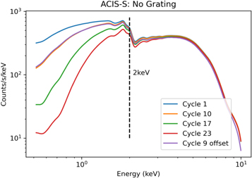
Figure 1. Simulated data of an on-axis source emitting a flat power law (Γ = 0, norm = 1) as seen with the ACIS-S camera for cycles 1, 10, 17, and 23. An off-axis source (2 786 from the center) is observed in cycle 9 as well.
Download figure:
Standard image High-resolution imageChandra observations may also be affected by vignetting when the source is observed off axis.
6
In particular, for sources farther than 5' from the center, there may be a significant softening of the spectrum due to stronger vignetting at higher energies. All of the observations used in this work have the sources of interest within 5' of on axis. Figure 1 also shows simulated data for an off-axis source (28 from the center) and the relative sensitivity is not significantly reduced until >8 keV where Chandra is already dominated by background counts. We conclude that the effects from effective area degradation or off-axis sources should not impact this method significantly.
We use data from the FPMA detector for the three sources with multiple NuSTAR observations. We note that there is no substantial difference between the counts observed with FPMA and FPMB, so we choose to consider only FPMA to avoid slightly higher background rates in the FPMB detector.
3. Method
3.1. Hardness Ratio (HR)
We define the HR to be

where H and S are the net counts (see Equation (2)) in the hard and soft bands, respectively. We use two sets of energy bands
These bands were chosen to optimize the ability to detect changes in NH due to torus structure by focusing on the energy range most sensitive to changes in absorption around  . In previous studies, the bands used are typically (0.5–2) keV for soft and (2–10) keV for hard. We find that these bands are not ideal for detecting changes in obscuration of already obscured sources with NH > 1022 cm–2 (see Figure 2). This is because the soft counts are all absorbed even at moderate obscuration levels, so there is no sensitivity at NH ⪆ 1023 cm−2. By focusing the hard and soft bands on the energies most affected by NH variability in the region of interest, the variability is more likely to be detected by the HR. Furthermore, ignoring energies <2 keV allows for comparison between all cycles of Chandra observations by avoiding the temporal degradation of sensitivity at soft energies.
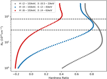
Figure 2. Calculated HRs for data simulated using the borus02 model for a range of NH values. HR2 continues to increase beyond NH ∼ 3 × 1023 cm−2 whereas HR1 loses sensitivity and eventually decreases. Neither is sensitive to changes in NH beyond NH ∼ 3 × 1024 cm−2 given the selected average torus properties.
Download figure:
Standard image High-resolution imageThe second HR, HR2, is needed to break a degeneracy present due to the increased importance of the reflection component in sources with high obscuration (see Figure 2). Above a certain NH, all of the primary soft counts are absorbed, leaving only the reflected counts visible. Since the reflection component does not depend on the line-of-sight NH, these highly obscured sources show softer HR1 as NH is increased, which decreases the sensitivity of HR1 in this NH region and ultimately strips it of its predictive power entirely. According to our simulations using the borus02 model, this occurs at NH ∼ 3 × 1023 cm−2 for AGNs with photon index, Γ = 1.9; average torus column density, NH,tor = 1024 cm−2; inclination angle  and covering factor cf
= 0.67 (values based on the results by Zhao et al. 2021 using a sample of ∼100 obscured AGNs having broadband X-ray coverage). Since HR2 is shifted to higher energies, it remains sensitive to NH variability at and beyond this limit as seen in Figure 2. It is important to note that these specific curves should only be taken as indicative since they are meant to represent an "average" AGN, and most individual sources will differ from these simulated data. However, the trends in Figure 2 should apply for any given source, because the average torus properties are not expected to change on the same timescales as the line-of-sight NH (see, e.g., Marchesi et al. 2022).
and covering factor cf
= 0.67 (values based on the results by Zhao et al. 2021 using a sample of ∼100 obscured AGNs having broadband X-ray coverage). Since HR2 is shifted to higher energies, it remains sensitive to NH variability at and beyond this limit as seen in Figure 2. It is important to note that these specific curves should only be taken as indicative since they are meant to represent an "average" AGN, and most individual sources will differ from these simulated data. However, the trends in Figure 2 should apply for any given source, because the average torus properties are not expected to change on the same timescales as the line-of-sight NH (see, e.g., Marchesi et al. 2022).
The net counts in each band are obtained from the reprocessed event file of Chandra observations and the cleaned pn event file for XMM-Newton observations. The source and background regions were set according to the procedure described in Torres-Albà et al. (2023). The CIAO 4.13 command dmextract was used to obtain the total counts in the source and background regions. The net counts is then calculated by

where Asrc is the area of the source region and Abkg is the area of the background region.
The errors on the total and background counts are calculated following the methods for Poisson statistics in Gehrels (1986). The approximate upper and lower single-sided limits for a measured number of counts n is given by Equations (9) and (14) in Gehrels (1986)
for a confidence level of 84.13%. This corresponds to the 1σ confidence interval for the number of counts. These limits are calculated for ntot and nbkg and the error δ n is taken to be the average difference 7 between the measured count and the upper and lower bounds

The total error on the net counts is then

This net count error is propagated through to the HR to get the 68% confidence error on the HR

where H and S are the net counts, nnet, in the "hard" and "soft" bands respectively.
3.2. Cross-instrument Comparison
The ability to compare observations across multiple instruments is essential to maximize the opportunities for variability detection. Many AGNs do not have multiple observations taken by the same instrument, so to study them over large periods requires comparing observations from multiple telescopes. Our sample would have only 43 pairs of observations if we were to avoid cross-instrument comparisons, as opposed to the 72 pairs we have, given a proper comparison between instruments.
It is clear that this method should work when comparing Chandra observations with different Chandra observations, but it is not as simple when comparing Chandra with XMM-Newton. In this case, the differences in the instrument response functions make it impossible to compare the raw HRs between instruments meaningfully (Park et al. 2006; Peretz & Behar 2018). Therefore, a method must be developed to correct for these differences.
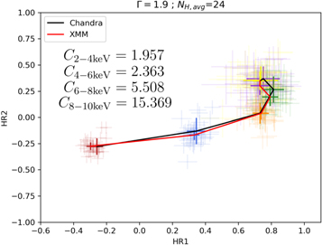
In order to overcome the difficulty in comparing Chandra to XMM-Newton observations, we must account for the differences in the shapes of the instrument response. In particular, the steep decline of the ACIS-S response with respect to the EPIC pn response beyond ∼4 keV and the lack of response in ACIS-S beyond ∼7 keV. This is shown in Figure 3. Figure 4 shows data simulated with the borus02 model for NH values ranging from 9 × 10²¹ to 8 × 1023 cm−2. As expected, the HRs measured by Chandra are systematically softer than those measured by XMM-Newton, especially HR2.
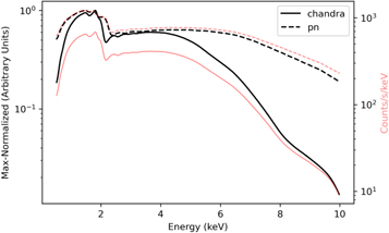
Figure 3. Spectra simulated for Chandra and XMM-Newton using the same method as in Figure 1. This is equivalent to the shapes of the responses for the ACIS-S and EPIC pn cameras, respectively. The red lines show the data on an absolute scale and the black lines show a normalized scale. The Chandra data have a much lower response in the hard band (4–10 keV) than pn, which need to be corrected.
Download figure:
Standard image High-resolution image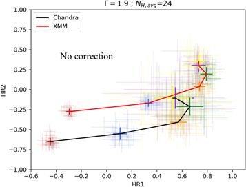
Figure 4. Uncorrected HRs for 20 spectra simulated with borus02 (Γ = 1.9;  ) for different levels of obscuration. The shaded error bars represent individual spectra while the solid error bars represent the mean values for the 20 spectra at a given NH. The colors red, blue, orange, green, purple, and yellow represent NH = (0.9, 10, 30, 50, 70, 80) × 1022 cm–2, respectively. The black line connects Chandra simulated data and the red line connects XMM-Newton simulated data.
Download figure:
Standard image High-resolution imageTo correct for this difference, we multiply the counts by correction factors in four different energy bands each 2 keV wide. These correction factors are calculated as the ratio of the count rate in each band of the EPIC pn response to the ACIS-S response shown as the red lines in Figure 3. The factors we obtain are

The HR and error are calculated in the same way as before, however, the hard counts are now the sum of the corrected counts in the bands contained in the hard band. For example, let a be the net counts in 2–4 keV, b the net counts in 4–6 keV, and so on. The total corrected counts are then T1 = Ca a + Cb b + Cc c + Cd d for HR1 and T2 = Cb b + Cc c + Cd d for HR2, where Ci is the correction factor corresponding to the appropriate band. Now, the HRs are
Similarly, the errors are
The results with these correction factors used on the simulated data are shown in Figure 5. This is an improvement in both HR1 and HR2 with all the corrected Chandra HRs being consistent with XMM-Newton HRs within the errors.
Download figure:
Standard image High-resolution imageWe also performed a test for model dependence. We simulated data for all combinations of photon index Γ = 1.6, 1.9, and 2.2 and  . The results show that there is no difference in the efficacy of these correction factors based on the model parameters. We conclude that these corrections are valid for the entire range of photon indices and reflection strengths that we expect to see. Thus, applying these corrections will allow us to compare a Chandra observation to a XMM-Newton observation for a given source more reasonably.
3.3. NuSTAR
There are three sources in our sample with multiple NuSTAR observations and we applied a modified version of our method to these. The energy bands used to define the HR for the NuSTAR observations are

Since the soft band in this definition covers most of the photons typically absorbed by even highly obscured AGN (<10 keV; Koss et al. 2016), there is no need to introduce a second set to break degeneracies.
3.4. Prediction of NH Variability
It is clear from Figure 2 that the HR should depend on NH. In this analysis, we flag a pair of observations as variable by calculating the χ2 of each pair of HR values assuming no variability. That is
where δHR is the 1σ error and μ is the mean HR of the two observations a and b. The source is flagged as variable if  . For example, if we consider a threshold
  , the source is flagged as variable if
  for either HR1 or HR2. This value corresponds to a significance level of α = 0.1. Thereby, we say that the observations are not consistent with each other at the 90% confidence level.
We compare these flagged observations to the "true" variable observations in Torres-Albà et al. (2023). Torres-Albà et al. (2023) obtained 90% confidence intervals for NH and these are considered variable if the confidence regions do not share any common NH values. We decide to use a simple discrepancy in the NH confidence regions because the asymmetric errors complicate the χ2 calculation.
We recognize that χ2 statistics do not necessarily apply in this instance, and therefore the significance level for variability in the HR likely does not correspond to the same significance level for variability in NH. However, as is discussed below, this quantity proves to be a reliable measure and is furthermore easily changed to adjust the sensitivity of our predictions.
4. Results and Discussion
4.1. XMM-Newton and Chandra Results
In total, we had 72 pairs of observations to test our method on and each observation has an NH value from each of the three models. Since this is a binary classification (variable or not variable), a confusion matrix is one of the best ways to analyze the reliability of the method (Stehman 1997). We consider a true positive (TP) to be when our method predicts variability and the NH values show variability. A false positive (FP) is when our method predicts variability, but the NH values are consistent with each other. A true negative (TN) and false negative (FN) are defined similarly.
4.1.1. Accuracy, Precision, and Recall
The simplest measure of reliability would be accuracy, which is defined as the total number of correct predictions divided by the total number of predictions. In terms of confusion matrix values

The accuracies for each of the three models are shown in Table 3.
Table 3. Accuracy, Precision, and Recall in Determining Variability, Using NH values from Each of the Three Models for Selected Threshold  Values
| Accuracy | ||||||
|---|---|---|---|---|---|---|
| Model |

|

|

|

|

|

|
| borus02 | 0.76 | 0.75 | 0.72 | 0.72 | 0.71 | 0.64 |
| MYTorus | 0.69 | 0.74 | 0.79 | 0.79 | 0.81 | 0.74 |
| UXCLUMPY | 0.74 | 0.72 | 0.81 | 0.81 | 0.79 | 0.72 |
| Precision | ||||||
| Model |

|

|

|

|

|

|
| borus02 | 0.77 | 0.78 | 0.84 | 0.86 | 0.92 | 0.94 |
| MYTorus | 0.59 | 0.63 | 0.74 | 0.76 | 0.83 | 0.82 |
| UXCLUMPY | 0.68 | 0.68 | 0.84 | 0.86 | 0.92 | 0.94 |
| Recall | ||||||
| Model |

|

|

|

|

|

|
| borus02 | 0.83 | 0.78 | 0.63 | 0.61 | 0.54 | 0.39 |
| MYTorus | 0.87 | 0.87 | 0.77 | 0.73 | 0.67 | 0.47 |
| UXCLUMPY | 0.86 | 0.80 | 0.74 | 0.71 | 0.63 | 0.46 |
Download table as: ASCIITypeset image
Accuracy can be a useful first approximation to the reliability of a method, however, it can hide particular behaviors that are important to note before applying this method to a larger sample. For example, if the sample contains mostly nonvariable observations, then a good accuracy can be obtained by simply never predicting variability. The prevalence quantifies how biased the original sample is toward variable or nonvariable observations and is defined as

If the sample contains more variable sources than nonvariable, then prevalence > 0.5. The prevalence for each of the three models is 0.57, 0.42, and 0.49 for borus02, MYTorus, and UXCLUMPY, respectively. Therefore, the sample used here is reasonably balanced, however, in the actual application of this method, the prevalence will not be known.
Precision and recall can be used to supplement the information given by the accuracy. These measures can provide a more nuanced interpretation of the results when considered along with accuracy. Precision is a measure of how good the classifier is at avoiding FPs and is defined as

Recall is a measure of how good the classifier is at finding TPs and is defined as

The precision and recall for the three models are also shown in Table 3.
Ideally, both of these values would be as close to 1 as possible. However, realistically, this is not achievable and one might want to prioritize one metric over the other. For example, if studying NH variability in a large sample of sources is the primary goal, precision might be valued over recall to avoid carefully fitting the X-ray spectra of observations that are not variable. On the other hand, if working from a smaller sample, FPs might not be as inconvenient. In this case, one would want to prioritize recall to make sure most of the variable sources are actually flagged. Furthermore, if the HRs are changing, this means that the spectral shape is changing and could indicate something interesting even if it does not happen to be a changing NH. For example, changes in the photon index are typically associated with variability of the AGN Eddington ratio, with higher accretion rates corresponding to a softer X-ray spectrum (Lu & Yu 1999; Shemmer et al. 2008; Risaliti et al. 2009b).
4.1.2. Receiver Operating Characteristic
Similar to precision and recall, one can define the false positive rate (FPR) and true positive rate (TPR). The FPR is the ratio of FPs to the total number of actual negatives and is defined as

The TPR is the ratio of TPs to total actual positives and is equivalent to recall (Equation (14)). In receiver operating characteristic (ROC) curves, the TPR is plotted against the FPR and therefore again provides a measure of how sensitive we are to TPs and how resistant we are against FPs (Fawcett 2006). A perfect classifier would be at the point (0, 1) while a random classifier would be along the line TPR = FPR. The curve is obtained by varying the decision threshold.
Figure 6 shows the ROC curves for each of the three models. Different  values were used to change the flagging sensitivity and obtain the ROC curves. The values used are
  = [0.016, 0.455, 2.706, 3.841, 6.635, 7.879, 10.828, 19.511], which correspond to confidence levels of [10%, 50%, 90%, 95%, 99%, 99.5% 99.9%, 99.999%]. The stars point out the location of the
  and
and  results for each of the models. Here we see that at the 90% confidence level, the TPR is over ∼0.8 while the FPR is under ∼0.4. This is representative of the high recall and average precision shown in Table 3. Interestingly, one can increase
  and the FPR still decreases faster than the TPR, representative of the high precision and average recall in Table 3.
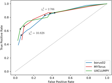
Figure 6. ROC curves for all three models. The threshold χ2 used in calculating the TPR and FPR increases from right to left along the lines. The stars represent the location of two of the threshold  values shown in the tables and confusion matrices. The gray dotted line represents a theoretical classifier with no predictive value. A larger distance from this line represents a more reliable classifier.
Download figure:
Standard image High-resolution imageIn general we see that for all combinations the predictive value is much better than random guessing. A quantity that measures the overall reliability of the classifier is the area under the ROC curve (AUC). We calculate AUC = 0.82, 0.81, and 0.84 for borus02, MYTorus, and UXCLUMPY, respectively. These values indicate a good classifier for this purpose.
More usefully in some circumstances, we note that as the threshold is increased up to  , corresponding to a confidence level of 99.9%, the FPR becomes small while the TPR remains >0.5. Specifically, at
  , (FPR, TPR) = (0.06, 0.54), (0.10, 0.63), and (0.06, 0.59) for borus02, MYTorus, and UXCLUMPY, respectively. This means that by decreasing our sensitivity to variability, we can reduce the number of FPs to almost zero, and still be able to detect more than half of the positive cases. This can be very useful in creating a sample of observations that are almost certain to show variability in NH. See Appendix A for the confusion matrices.
4.2. NuSTAR Results
The results for the three NuSTAR sources are shown in Figure 7. These plots show the best-fit NH value obtained from the UXCLUMPY model against the single HR defined in Section 3.3 for NuSTAR data.
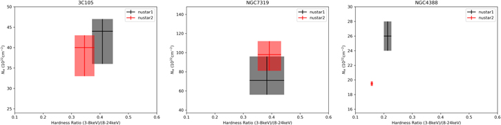
Figure 7. Direct comparison of the best-fit NH values from UXCLUMPY to the NuSTAR HR. As can be seen, the HR is able to predict NH variability in NGC 4388 and nonvariability in 3C 105 and NGC 7319.
Download figure:
Standard image High-resolution imageThe predictions are correct for all three sources. For 3C 105, the value for the HR fit is  , indicating no variability, and indeed, there is no NH variability measured between the observations. Similarly, for NGC 7319,
  . For the variable source NGC 4388,
  , indicating large variability. These predictions are not included in the results shown in Table 3 or Figure 6 since the prediction method is not the same.
Although the sample size is very small, the NuSTAR HR seems to be better at predicting NH variability. It would not be surprising if this is the case, considering the energy bands we are able to use with NuSTAR might be better aligned to detect changes in line-of-sight absorption in z ∼ 0 obscured AGNs. This could be due to the fact that increasing NH only significantly affects the 3–8 keV band, which leads to a predictable increase in HRnu. On the other hand, for HR1 and HR2, an increase in NH affects both energy bands differently depending on the amount of absorption and reflection, leading to a less predictable change in the HRs.
5. Simulations
To verify the reliability of this method, we apply it to samples of simulated spectra with different model configurations and count levels. For simplicity, we use the borus02 model to simulate XMM-Newton spectra for NH values ranging from NH = 1023 cm−2 to NH = 1.1 × 1024 cm−2 in increments of 5 × 1022 cm−2, which is the range of values to which we are interested in applying the method. The photon index is Γ = 1.9, the average torus column density is NH,avg = 1024 cm−2, and the covering factor is cf
= 0.67, as they were in Section 3. We also consider two different inclination angles,  , representing an edge-on torus and
  , representing the average inclination angle for a large sample of sources with inclination angles distributed randomly. We consider six different brightness levels in which the total number of counts in the 2–10 keV band range from ∼100, 500, 1000, 5000, 10,000, and 20,000.
Figure 8 shows the results in the HR1−HR2 plane for spectra with ∼1000 counts, which is the typical number of counts in our sample observations discussed above. This indicates that our method can detect small variability (∼5 × 1022 cm−2) in lower-obscuration sources. For the highest-obscuration sources considered here, a change in NH of closer to ∼5 × 1023 cm−2 is needed for a reliable detection (see Figure 10). Furthermore, this plot indicates that while there is some scatter in the HRs at a given NH, the method is reliable at avoiding FPs (see Figure 9). The results for the other count levels and the edge-on case are shown in Appendix B. As expected, the method improves when the observations have higher counts. The edge-on case shows similar results regarding the dependence on count levels. However, the shape of the NH dependence is different because the soft counts from reflection off of the far side of the torus are no longer present and the spectrum does not soften for highly obscured scenarios.
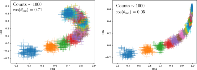
Figure 8. The HR1 and HR2 values along with the associated 68% errors for simulated spectra with 1000 counts in the 2–10 keV energy range. The colors represent different NH values starting at NH = 1023 cm−2 and ending at NH = 1.1 × 1024 cm−2 in increments of NH = 5 × 1022 cm−2. The 10 colors shown cycle through in the same order. There are 100 spectra simulated for each NH value. The HRs change predictably with NH along the trend lines, so there is no confusion. The left panel shows the case for an inclination angle θinc = 45°, which is the typical inclination angle expected for a random distribution of orientations. The right panel shows the edge-on case with θinc = 87°.
Download figure:
Standard image High-resolution image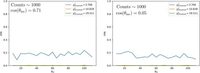
Figure 9. The FPR as a function of the NH for three different threshold  values. The left panel shows inclination angle θinc = 45°. The right panel shows inclination angle θinc = 87°. The blue line uses a threshold
  of 2.706, corresponding to 90% confidence. The FPR is ≲20% for all levels of obscuration in both cases. For the higher threshold
  values, the FPR drops essentially to zero.
Download figure:
Standard image High-resolution imageA plot of the FPR as a function of NH for three different threshold  values is shown in Figure 9. The same plot is shown for the different count levels in Appendix B. It is clear that the level of obscuration does not have a large impact on the FPR. Furthermore, the FPR is roughly the same regardless of the number of counts or the inclination angle as can be seen from the plots in Appendix B. This is likely due to the fact that as the counts decrease and the scatter increases, the errors also increase at the same rate, yielding a constant FPR. An interesting thing to note on these results is that the FPR for the simulated data is lower than the FPR for the Torres-Albà et al. (2023) sample. We have identified two potential explanations for this and we expect some combination is responsible for the discrepancy. First, in our simulations, we consider only variability in NH. In the real observations, other parameters may vary that can affect the HR, leading to an increase in the FPR over the simulated case. We will explore this in detail in a future publication (I. S. Cox et al. 2023, in preparation) to see which parameters are most important and try to quantify how prevalent these effects can be. Second, in the definition of FPR in Equation (15), the "true" and "false" predictions are relative to the NH values obtained through spectral fitting. This process is not infallible as determining NH variability by spectral fitting can itself have FNs. That is, NH variability may be detected by our HR method while not being detected with spectral fitting. This would result in a nominal FP in the HR method, increasing the FPR.
In Figure 10, we show the TPR as a function of the change in NH between two observations, ΔNH. The typical variability for the Torres-Albà et al. (2023) sample is shown as the vertical dashed line. This plot shows that at the "typical" variability (ΔNH ∼ 2.3 × 1023 cm−2) and "typical" count level (∼1000), we would expect to see a TPR of ∼0.8 at 90% confidence. Furthermore, with only 100 counts, we expect to detect ∼30%–50% of sources with typical variability (depending on the inclination angle) and with 500 counts, ∼60%–90%. These values are roughly consistent with the value obtained from the sample analysis above. The TPR is better in the edge-on case for a given count level and threshold  . This is likely due to the fact that photons from the far side of the torus are not contaminating the spectrum, and only the part of the torus responsible for absorption in the line of sight is visible. This would increase the sensitivity of changes in absorption over the case where parts of the torus that do not contribute to absorption are nonetheless contributing photons. However, we do not expect this geometry to affect the FPR, and this is confirmed by the simulations.
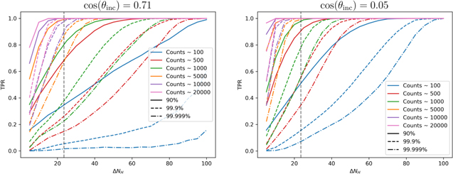
Figure 10. The TPR as a function of ΔNH. The left panel shows inclination angle θinc = 45°. The right panel shows inclination angle θinc = 87°. The colors show different count levels and the line styles show different sensitivity levels. This plot shows that the TPR increases with the number of counts and ΔNH. For observations with ≳5000 counts (orange line), we would expect to detect all variable events at 90% confidence, or a threshold  of 2.706 (solid line) in both cases.
Download figure:
Standard image High-resolution image6. Summary and Conclusion
In this work, we introduced a method to predict variability in line-of-sight NH for an AGN, without having to perform difficult and time-consuming spectral modeling, or even extract a spectrum. This method would allow the user to sift through many X-ray observations to quickly flag sources that are most likely to experience NH variability. These flagged sources can then be studied further by performing a full spectral fitting analysis to obtain accurate NH values.
To do this, we used variability in the HR as a proxy for variability in NH, which is commonly done. Two different HRs were defined to account for a possible degeneracy in highly obscured scenarios. Furthermore, a method to "correct" HRs from Chandra observations to match XMM-Newton observations using only easily obtainable counts was developed. This method can likely be used in many situations where one would like to compare HRs from different instruments without having to extract spectra. However, in this study, it has only been tested with Chandra and XMM-Newton in the 2–10 keV energy range.
We flag a pair of observations as variable if the χ2 fit, assuming no variability, is larger than a given threshold which can be set to a desired sensitivity. We first tested this prediction method on a sample of 12 sources with NH values determined through in-depth spectral analysis that used self-consistent physical tori models and a careful treatment of reflection. The ROC curve indicates that this method is effective at classifying variable versus nonvariable sources. Furthermore, the ability to adjust the sensitivity with the threshold χ2 value can allow the user to create a sample of sources that almost certainly have variability in the line-of-sight NH, however, this will be far from a complete sample. On the other hand, one could construct a sample containing almost all of the variable sources, while having to deal with a fair number of FPs. Using this method in its most conservative setting can also provide us an approximate lower limit on the fraction of local AGNs that display variable obscuration.
We also tested the method on simulated data with a range of count levels. We found that the reliability measures on the simulated data were consistent with the real data sample, except for a lower FPR, which is explained in Section 5. We found that the ability to detect variability decreases as the number of counts decrease (as expected) but the method remains better than random guessing for observations with as few as 100 counts.
We conclude that this method is an effective way to predict absorption variability between two observations of a given AGN. The fact that the sensitivity of this method can easily be adjusted to suit the requirements of a particular project makes this a very flexible tool to preselect samples of sources for absorption variability studies. We reiterate, this method is not to be used as a substitute for measuring the NH via spectral fitting. Rather, it is only an indicator of variability between two observations.
In a future paper (I. S. Cox et al. 2023, in preparation), we will apply this method to a larger sample of sources with unknown NH values. We will flag sources with a variable HR and study those with careful spectral fitting. Along with further constraining the physical parameters of the obscuring medium surrounding the AGN, this upcoming study will greatly improve the statistics in this work. Therefore, we will be able to understand the reliability of this method better before being overwhelmed with the amount of data from upcoming missions.
Acknowledgments
We thank the anonymous referee for their comments and suggestions which significantly improved this article. I.C., N.T.A, M.A., R.S., and A.P. acknowledge funding from NASA under contracts 80NSSC19K0531, 80NSSC20K0045, and 80NSSC20K834. S.M. acknowledges funding from the INAF "Progetti di Ricerca di Rilevante Interesse Nazionale" (PRIN), Bando 2019 (project: "Piercing through the clouds: a multiwavelength study of obscured accretion in nearby supermassive black holes"). The scientific results reported in this article are based on observations made by the X-ray observatories Chandra, NuSTAR, and XMM-Newton, and has made use of the NASA/IPAC Extragalactic Database (NED), which is operated by the Jet Propulsion Laboratory, California Institute of Technology under contract with NASA. We acknowledge the use of the software package HEASoft.
Appendix A: Confusion Matrices
Figures 11–13 show the confusion matrices for all three models with the three different sensitivity levels shown in Table 3. The diagonal of these matrices shows the correct predictions while the top right contains the FPs (nonvariable sources classified as variable) and the the bottom left contains the FNs (variable sources classified as nonvariable).
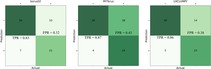
Figure 11. Confusion matrices for all three models at the 90% confidence level ( ). These show that the method is good at avoiding FNs, meaning that most of the variable sources in a sample will be flagged. However, this comes at the expense of flagging as variable more sources that are not variable (top right).
Download figure:
Standard image High-resolution image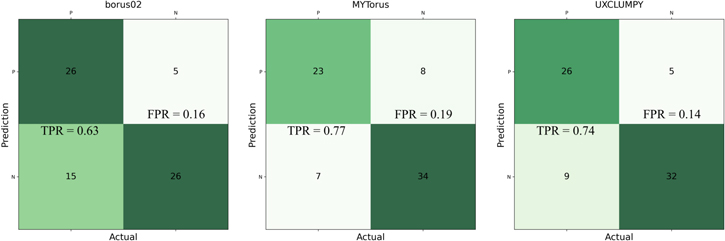
Figure 12. Confusion matrices for all three models at the 99% confidence level ( ). These show that at this sensitivity, the method does a decent job overall at flagging variable sources while avoiding nonvariable sources.
Download figure:
Standard image High-resolution image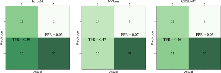
Figure 13. Confusion matrices for all three models at the 99.999% confidence level ( ). The small number of FPs (top right) show that, at this sensitivity, almost none of the nonvariable sources in a sample will be flagged. However, this comes at the expense of not selecting a larger number of variable sources (bottom left).
Download figure:
Standard image High-resolution imageAppendix B: Simulations
Figures 14 and 15 show the same thing as Figures 8 and 9 for the remaining count levels studied (100, 500, 5000, 10,000, and 20,000 counts). Figure 14 shows that the ability to distinguish different column densities with the HR values increases significantly as the count level increases. However, Figure 15 shows that the FPR is roughly independent of the number of counts, as expected from the discussion in Section 5. Since the FPR remains low even for observations with much fewer counts than those in the Torres-Albà et al. (2023) sample, it is likely that this method would still be able to place a lower limit on the fraction of variable sources in a sample regardless of the typical number of counts of the observations.
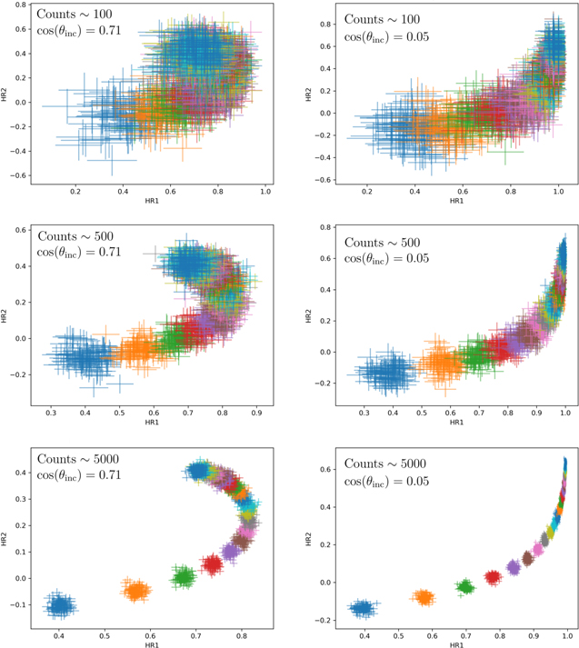
Download figure:
Standard image High-resolution image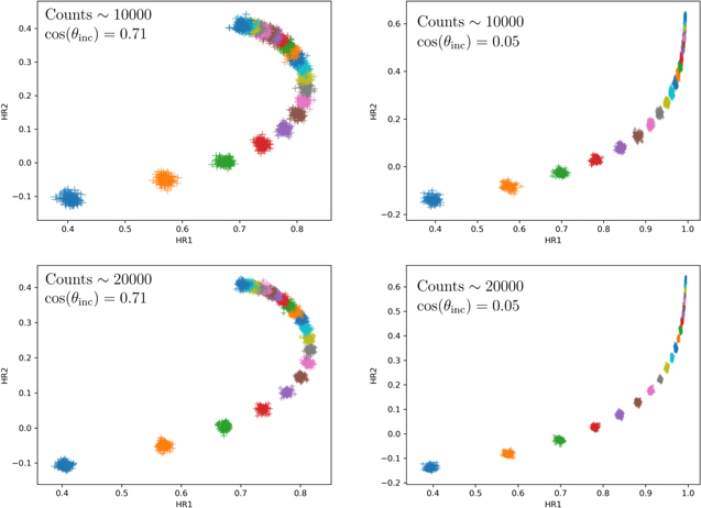
Figure 14. The HRs of simulated spectra for a range of NH values and different count levels. All spectra here were simulated as described in Section 5. The colors are the same as in Figure 8.
Download figure:
Standard image High-resolution image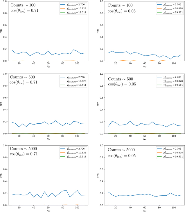
Download figure:
Standard image High-resolution image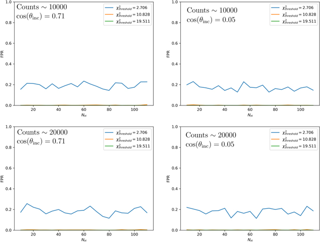
Figure 15. The FPR as a function of NH for three different threshold  values and different count levels. The details are described in Figure 9.
Download figure:
Standard image High-resolution image
Footnotes
- 6
See Figure 6.6 in the Chandra Proposer's Observatory Guide, https://cxc.harvard.edu/proposer/POG/html/index.html.
- 7
The asymmetry is very small or nonexistent in every case.