


Abstract
We present [C ii] 158 μm and [O i] 63 μm observations of the bipolar H ii region RCW 36 in the Vela C molecular cloud, obtained within the SOFIA legacy project FEEDBACK, which is complemented with APEX 12/13CO (3–2) and Chandra X-ray (0.5–7 keV) data. This shows that the molecular ring, forming the waist of the bipolar nebula, expands with a velocity of 1–1.9 km s−1. We also observe an increased line width in the ring, indicating that turbulence is driven by energy injection from the stellar feedback. The bipolar cavity hosts blueshifted expanding [C ii] shells at 5.2 ± 0.5 ± 0.5 km s−1 (statistical and systematic uncertainty), which indicates that expansion out of the dense gas happens nonuniformly and that the observed bipolar phase might be relatively short (∼0.2 Myr). The X-ray observations show diffuse emission that traces a hot plasma, created by stellar winds, in and around RCW 36. At least 50% of the stellar wind energy is missing in RCW 36. This is likely due to leakage that is clearing even larger cavities around the bipolar RCW 36 region. Lastly, the cavities host high-velocity wings in [C ii], which indicates relatively high mass ejection rates (∼5 × 10⁻⁴ M⊙ yr−1). This could be driven by stellar winds and/or radiation but remains difficult to constrain. This local mass ejection, which can remove all mass within 1 pc of RCW 36 in 1–2 Myr, and the large-scale clearing of ambient gas in the Vela C cloud indicate that stellar feedback plays a significant role in suppressing the star formation efficiency.
Export citation and abstract BibTeX RIS

Original content from this work may be used under the terms of the Creative Commons Attribution 4.0 licence. Any further distribution of this work must maintain attribution to the author(s) and the title of the work, journal citation and DOI.
1. Introduction
The interstellar medium (ISM) is a complex mixture of multiple phases (McKee & Ostriker 1977; Wolfire et al. 1995, 2003; Walch et al. 2015) where stars form in the densest regions (Bergin & Tafalla 2007), which are mostly organized in dense filaments (André et al. 2010; Molinari et al. 2010; Schneider et al. 2012). Feedback from the star formation process in the form of ionizing radiation and stellar winds provides substantial energy injection into the ISM, which can drive its chemical and dynamical evolution. Feedback might also play a significant role in suppressing the star formation rate (SFR) in molecular clouds. It has been proposed that massive stars form in gravitationally collapsing hubs and ridges (Motte et al. 2018), which results in the rapid accumulation of mass at the center of collapse (i.e., in a few freefall timescales). This would result in high SFRs, which are not observed, if not counteracted by feedback processes (e.g., Mac Low et al. 2017; Vázquez-Semadeni et al. 2019). Additionally, with astrophysical simulations it remains extremely challenging to predict the impact and role of the different stellar feedback processes on the molecular cloud evolution because of the large computational requirements and complex subgrid physics (e.g., Dale et al. 2014; Geen et al. 2020; Grudić et al. 2021; Kim et al. 2021).
Stellar feedback leads to the formation of H ii regions, which come in the form of H ii bubbles (Churchwell et al. 2006; Deharveng et al. 2010; Beaumont & Williams 2010; Kendrew et al. 2012), bipolar H ii regions (Bally & Scoville 1982; Deharveng et al. 2015; Schneider et al. 2018; Samal et al. 2018), and more irregular features (Anderson et al. 2011, 2014). Recently, the kinematics of a couple of H ii bubbles have been studied with the [C ii] 158 μm fine-structure line (Anderson et al. 2019; Pabst et al. 2019, 2020; Luisi et al. 2021; Tiwari et al. 2021; Beuther et al. 2022) because it traces the photodissociation regions (PDRs) at the interfaces between H ii regions and molecular clouds, where mostly far-ultraviolet (FUV) photons in the energy range of 6–13.6 eV regulate the physical conditions of the ISM (Hollenbach & Tielens 1999). The [C ii] kinematics in some of these regions demonstrated the presence of expanding shells with velocities up to 15 km s−1 (Pabst et al. 2019, 2020; Luisi et al. 2021; Tiwari et al. 2021; Beuther et al. 2022). However, they often show expansion in only one direction, mostly blueshifted, which suggests that the bubbles might not be fully spherical. This more complex geometry is important for the interpretation of the various emission distributions. Observations of hot X-ray-emitting plasmas, produced by stellar winds from OB stars, showed that these plasmas have an unbalanced energy budget, i.e., the energy of the hot plasmas is significantly lower than the energy injected by stellar winds (e.g., Townsley et al. 2003, 2006, 2011; Harper-Clark & Murray 2009; Lopez et al. 2011, 2014; Rosen et al. 2014; Tiwari et al. 2021). The more complex geometry of expanding H ii regions could thus allow the hot plasma to leak out of the region, which might explain the mismatch in the energy budget. The lack of an expanding shell at one side of a region leading to rapid hot plasma leakage was recently demonstrated for RCW 49 by Tiwari et al. (2021). Studying the [C ii] emission dynamics can also help to constrain the role of stellar feedback in suppressing the star formation of a molecular cloud, as well as triggering a second generation of star formation, which is still highly debated (e.g., Zavagno et al. 2010, 2020; Dale et al. 2013; Walch et al. 2015). Luisi et al. (2021) proposed, based on [C ii] data taken within the Stratospheric Observatory for Infrared Astronomy (SOFIA) legacy program FEEDBACK 12 (Schneider et al. 2020), that star formation is triggered in RCW 120. They propose a model in which a wind-driven expanding [C ii] shell sweeps up a gas shell that fragments and forms stars on very short timescales (∼0.1 Myr).
The formation of bipolar H ii regions has received less attention than single bubbles, which might be related to the fact that bipolar H ii regions are not as common (e.g., Samal et al. 2018). Early work by Bodenheimer et al. (1979) demonstrated that a bipolar H ii region can form by expansion in a flattened molecular cloud, consistent with simulations by Wareing et al. (2017). Whitworth et al. (2018) proposed that bipolar H ii regions emerge from a sheet that was formed by a cloud–cloud collision, whereas Kumar et al. (2020) propose that bipolar H ii regions form from a hub-filament cloud that was flattened by rotation. Numerical simulations predict that a significant fraction of the dense molecular gas is organized in filaments and sheets (e.g., Padoan et al. 2001; Vázquez-Semadeni et al. 2006; Banerjee et al. 2009; Wareing et al. 2019), allowing for the formation of bipolar H ii regions. This view of the molecular ISM organized in filaments and sheets is now increasingly supported by observations (e.g., André et al. 2014; Qian et al. 2015; Tritsis & Tassis 2018; Shimajiri et al. 2019; Bonne et al. 2020a).
Here we focus on the bipolar H ii region RCW 36, which is located in the dense ridge of the Vela C molecular cloud (Hill et al. 2011; Minier et al. 2013; Fissel et al. 2016). The distance of the Vela C molecular cloud has recently been updated to 900 ± 50 pc with the GAIA data (Gaia Collaboration et al. 2018; Zucker et al. 2020). Earlier distance estimates (Liseau et al. 1992; Yamaguchi et al. 1999; Massi et al. 2019) derived values between 700 and 1000 pc. RCW 36 is probably the first developing H ii region in Vela C, which is well illustrated by Figure 1 in Hill et al. (2011), suggesting that Vela C is still in a relatively early stage of star formation. The young cluster at the origin of the bipolar cavities has more than 350 stars located within a radius of 0.5 pc (Baba et al. 2004), has an estimated age of 1.1 ± 0.6 Myr (Ellerbroek et al. 2013a), and is proposed to host two O stars of type O9.5V and O9V (Massi et al. 2003; Bik et al. 2005; Ellerbroek et al. 2013a). This is consistent with the estimated total luminosity of 1.3 × 10⁵ L⊙ for the cluster (scaled to the adopted distance in this work: d = 900 pc; Verma et al. 1994). Herschel observations indicated that the young cluster is surrounded by a dense molecular ring of swept-up gas with a radius of ∼1 pc, which is proposed to expand with a velocity of 1–2 km s−1 (Minier et al. 2013). In Figure 1, the Hα absorption in the eastern part of the ring would then suggest that this part of the ring is expanding toward us and that the western part is expanding away from us (Minier et al. 2013). Multiwavelength observations of RCW 36 have also established the presence of several protostar and young stellar object (YSO) candidates (Bik et al. 2006; Ellerbroek et al. 2011; Hill et al. 2011; Giannini et al. 2012; Massi et al. 2019), indicating relatively low mass ongoing star formation in the region, as well as the presence of two Herbig-Haro (HH) jets (Ellerbroek et al. 2013b).

Figure 1. Left: the Herschel 70 μm map of RCW 36 (Minier et al. 2013). The red box outlines the region that was already observed for the FEEDBACK program, and the dashed white box shows the area that will be mapped. The blue crosses mark the location of the two O-star candidates. Note that the close proximity of the two O-star candidates does not allow us to distinguish them clearly in this figure. The black dashed ellipse indicates the location of the central molecular ring, first reported by Minier et al. (2013). The Herschel 70 μm map also traces the limb-brightened shells at the cavity walls. The white contours indicate the Herschel column density at  = (1, 2, 4, 8) × 1022 cm−2 determined using the method presented in Palmeirim et al. (2013). Right: Hα intensity map toward RCW 36 from the SuperCOSMOS Hα Survey. The intensity units of the map are not calibrated to a specific unit and are only relative (Hambly et al. 2001; Parker et al. 2005). The white contours again indicate the Herschel column density.
Download figure:
Standard image High-resolution imageIn this paper, we present the first [C ii] and [O i] observations of RCW 36 obtained by the SOFIA FEEDBACK Legacy survey in combination with complementary data to acquire a global understanding of the evolution of this region. Both the [C ii] and [O i] lines are PDR tracers, where [O i], with a critical density of 5 × 105 cm−3, is particularly used to trace dense PDRs (Röllig et al. 2006). These FEEDBACK observations unveil new dynamical information that was not available before. Section 2 describes our new [C ii], [O i], and CO (3–2) observations, as well as archival X-ray and submillimeter continuum data sets. The results of these observations are presented in Section 3. In Section 4, the expansion energetics and mass ejection parameters are calculated, and in Section 5 the [C ii] data are compared with Chandra X-ray observations of RCW 36. In Section 6, these results are combined to propose a scenario for the evolution of RCW 36, and we discuss the results in the global context of stellar feedback on molecular clouds.
2. Observations
2.1. SOFIA
The FEEDBACK C+ Legacy survey observed the [C ii] 3
P3/2 → 3
P1/2 transition, at 158 μm, and [O i] 3
P1 → 3
P2 transition, at 63 μm, simultaneously with the upGREAT instrument (Risacher et al. 2018) on board the airborne SOFIA (Young et al. 2012) during a flight on 2019 June 6 from Christchurch, New Zealand. The observation strategy was to carry out [C ii] and [O i] on-the-fly (OTF) maps and is described in detail in Schneider et al. (2020). For RCW 36, the planned map within the legacy program has a size of 14 4 × 144, indicated in Figure 1. Here we present the lower part of the map (144 × 72) that has been observed so far. The center of the full map is located at α(J2000) = 08h59m26
 8 and δ(J2000) = −43° 44'14
 1, and the emission-free OFF position is at α(J2000) = 09h01m317 and δ(J2000) = −43°22'500.
Both the reduced [C ii] (smoothed to 20'') and [O i] (smoothed to 30'') maps, used in this paper, have a spectral binning of 0.2 km s−1. The typical noise rms of these smoothed data within 0.2 km s−1 is 0.8–1.0 K for [C ii] and ∼0.8–1.5 K for [O i]. The calibration was done using the GREAT pipeline (Guan et al. 2012). To convert the antenna to main-beam temperatures, a forward efficiency ηf = 0.97 and main-beam efficiency ηmb = 0.65 for [C ii] and 0.69 for [O i] were applied. To improve the baseline removal of the data, a new method based on principal component analysis (PCA) was used (C. Buchbender et al. 2022, in preparation). This technique was also employed for the data published in Luisi et al. (2021), Tiwari et al. (2021), and Kabanovic et al. (2022). Specifically, PCA identifies the systematic components of baseline variation in different spectra, which allows us to accurately remove them and recover the actual spectrum. For a more general overview of PCA we refer the reader to Jolliffe (2011).
2.2. APEX
Complementary 12CO (3–2) and 13CO (3–2) data were simultaneously obtained with the LAsMA 7-pixel receiver on 2019 September 27 and 2021 July 21 in good weather conditions (precipitable water vapor (pwv) ≈1 mm) using the APEX telescope
13
(Güsten et al. 2006). This heterodyne spectrometer allows simultaneous observations of the two CO isotopomers in the upper (12CO (3–2) at 345.7959899 GHz) and lower (13CO (3–2), 330.5879653 GHz) sidebands of the receiver. The LAsMA back ends are fast Fourier transform spectrometers (FFTSs) with 2 × 4 GHz bandwidth (Klein et al. 2012) and a native spectral resolution of 61 kHz. The main-beam size of the APEX observations (θmb= 182 at 345.8 GHz) is similar to the resolution of the [C ii] data. The mapped field with a size of 20' × 15' was scanned in total power on-the-fly mode, with a spacing of 9'' between rows (while oversampling to 6'' in scanning direction, R.A.). The map data were calibrated against a sky reference position at α(J2000) = 09h01m317 and δ(J2000) = −43° 22'500. For the APEX observations, a first-order baseline was removed, and a main-beam efficiency ηmb = 0.68 was used to convert the antenna temperatures to main-beam temperatures. The baseline-subtracted spectra have been binned to a spectral resolution of 0.2 km s−1. The final data cubes (with a pixel size of 91) have an rms of 0.45 K.
2.3. Ancillary Data
The Chandra X-ray Observatory ACIS camera (Garmire et al. 2003) observed a 17' × 17' field centered on RCW 36 for ∼70 ks in 2006. The MYStIX project (Kuhn et al. 2013) found 502 X-ray point sources in this field. These were excised, and the remaining data smoothed, to obtain an 0.5–7 keV diffuse X-ray image of the field (Townsley et al. 2014). ACIS is an intrinsic spectrometer, tagging every X-ray event with its energy and its position. We will use the Chandra/ACIS data to study the X-ray spectra in a variety of regions in and around RCW 36.
The RCW 36 region, being part of the Vela C molecular cloud, was observed with the PACS (Poglitsch et al. 2010) and SPIRE (Griffin et al. 2010) bolometers on the Herschel telescope as part of the Herschel imaging survey of OB young stellar objects (HOBYS) program (Motte et al. 2010). In this work, we use the flux map at 70 μm with an angular resolution of ∼6'', as it clearly outlines the bipolar H ii region. Further, we use the dust temperature map at 36'' resolution and a dust column density map at 182 resolution. This dust temperature and column density map was obtained by fitting the spectral energy distribution (SED) to the 160–500 μm data, using the method presented in Palmeirim et al. (2013).
We further make use of data from the WISE telescope from 3.4 to 22 μm (Wright et al. 2010), an Hα map of RCW 36 from the Southern Hα Sky Survey Atlas (SHASSA; Gaustad et al. 2001), and a large-scale dust polarization map at 500 μm with a spatial resolution of  that was observed with the BLASTPol balloon-borne receiver (Fissel et al. 2016, 2019; Gandilo et al. 2016).
3. Results
3.1. The Integrated Intensity Map
Figures 2 and 3 present the integrated intensity map for [C ii] and [O i], respectively. [C ii] is brightest toward the region that is surrounded by the high column density ring and shows more extended emission toward the two cavities. Outside of the cavity walls, the [C ii] intensity decreases rapidly. [O i], on the other hand, is only detected toward the high column density ring, where a high-density PDR can be expected.

Figure 2. The middle panel shows the line-integrated intensity map of [C ii] from −20 to 20 km s−1, with the white contours indicating the Herschel column density  at (1, 2, 4, 8) × 1022 cm−2. The [C ii], [O i], 12CO (3–2), and 13CO (3–2) spectra at the indicated positions are shown around the map. These spectra are named after their position in the map. The spectra from the central molecular ring are indicated with a "C," the spectra to the east with an "E," and the spectra to the west with a "W." The spectra indicate the presence of multiple velocity components and show signatures of self-absorption toward the ring (C). In several spectra (C1–C3), high-velocity blue- and redshifted wings are detected. The spectrum "W3" at the top right highlights the color legend for the spectra. When inspecting the spectra, note that the y-scale is different in each subpanel.
Download figure:
Standard image High-resolution image
Figure 3. The integrated intensity map of [O i] at 63 μm from −20 to 20 km s−1, with the white contours indicating the column density  at (1, 2, 4, 8) × 1022 cm−2.
Download figure:
Standard image High-resolution imageThe line-integrated intensity maps of 12CO (3–2) and 13CO (3–2), presented in Figure 4, show a different structure. The emission follows the ring-like Herschel dust column density maps rather closely and shows that the CO emission is brightest at the edge around the bright [C ii] emission, which would be expected for a PDR irradiated by the central cluster. This is not a resolution effect since both beams have similar spatial resolution. To the southwest of the ring there is a region (local peak in dust column density) where the ring is significantly less bright in 12CO (3–2) and 13CO (3–2) (by a factor 2–3), but the [C ii] contours show a protrusion toward the west. This may indicate that there is a puncture in the ring so that the [C ii]-emitting gas can freely expand into a lower-density region, driven by the stellar feedback from the east. On the other hand, the weaker CO emission at this location (C3 in Figure 2) can be partly caused by self-absorption. This self-absorption can be related to the protrusion, as it would give rise to warm and cold gas layers along the line of sight, while there still appears to be a significant column density based on the Herschel data. On a larger scale outside the ring in Figure 4, 12CO (3–2) shows filamentary emission that is perpendicular to the dense ring. Several of these filamentary structures are also detected in [C ii] and show a curvature that appears to originate in the central cluster. This suggests that preexisting filaments are being swept up.
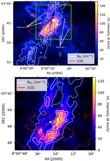
Figure 4. Top: the integrated 12CO (3–2) emission map from −20 to 20 km s−1, with Herschel column density contours in white and [C ii]-integrated intensity contours starting at 50 K km s−1 with increments of 100 K km s−1 in red to delineate their structure. Outside the molecular ring, the 12CO (3–2) emission shows filamentary structures that are oriented perpendicular to the ring (indicated by the white arrows). Bottom: same as the top panel, but for 13CO (3–2), in the green box indicated in the figure above, which follows the column density contours of the high column density ring closely. The [C ii] emission shows a structure perpendicular to the high column density ring in the southwest at the location where there is a drop in 13CO (3–2) intensity. The white crosses indicate the location of the two O-star candidates.
Download figure:
Standard image High-resolution imageRecently, [C ii]-integrated intensity observations at an angular resolution of 90'' were presented in Suzuki et al. (2021) using a 100 cm balloon-borne infrared telescope. Smoothing the FEEDBACK-integrated intensity map to a resolution of 90'', presented in Appendix A, the results look extremely similar to the maps presented in Suzuki et al. (2021). The intensity maps appear to agree within 10%, which corresponds to typical calibration errors. Comparing the smoothed map in Figure 20 with the FEEDBACK map in Figure 2, it is evident that the higher spatial resolution of the SOFIA observations is necessary to resolve, e.g., the ring and filamentary structures in [C ii]. Another major advantage of the FEEDBACK observations is the high spectral resolution of the observations, which allows us to study the dynamics of the region.
3.2. Multiple Velocity Components, Absorption, and High-velocity Wings
The [C ii], CO, and [O i] spectra shown in Figure 2 are all very complex and cannot be described by a single Gaussian velocity component. The bulk emission of the molecular cloud/dense ring is best traced with the 13CO (3–2) line that is visible for all center positions (C1–C5) around 7–8 km s−1 but mostly absent for all western (W1–W3) and eastern (E1–E2) positions. The 12CO (3–2) line profile shows significant variation depending on the position. For the spectra at the central molecular ring, we observe two apparent line components that are caused by foreground or self-absorption because the 13CO line peaks in the 12CO dip at ∼7 km s−1. Note that the optically thin dense gas tracers N2H+ (2–1) and NH3(1,1), presented in Fissel et al. (2019), also peak at velocities around 7–8 km s−1. The absorption thus mimics two separate velocity components that were interpreted by Sano et al. (2018) as two velocity components tracing a cloud–cloud collision. We observe that the absorption in 12CO continues toward the east and west because the dip in the line profile is always around 7 km s−1 and the 13CO emission clearly peaks in the 12CO dip for position W1 (but is too weak for W2, E1, and E2). For all center positions, the self-absorption is dominant toward the blueshifted part of the main velocity component, which is generally associated with expansion (e.g., Castor & Lamers 1979).
The [C ii] line has a bright, prominent component (main-beam temperatures up to ∼100 K for the center positions) around 8–9 km s−1. This bright component is also found in the eastern spectra but is less strong for the three western positions (W1–W3). This component is also affected by absorption, which we can prove with our [13C ii] line observations shown in Figure 5 and Appendix B. The intensity of the [C ii] main component drops where [13C ii] has its emission peak, similar to what was observed for several other bright [C ii] sources with SOFIA (e.g., Graf et al. 2012; Guevara et al. 2020; Kirsanova et al. 2020; Mookerjea et al. 2021; Kabanovic et al. 2022). There is also a separate second velocity component between 0 and 5 km s−1 (hereafter the blueshifted component), which is well visible in [C ii] and even brighter than the 7–8 km s−1 component in the west of the ring (W1–W3). At some locations (C3, C4, W3) this component is also detected in 12CO (3–2) (see Figure 2), but mostly at slightly higher velocities (3–5 km s−1).

Figure 5. The [13C ii] F = 2–1 line emission (magenta), averaged over the dense molecular ring, compared to the [C ii] line profile (blue), which is averaged over the same area. Even though there is confusion by the redshifted high-velocity wing seen with [C ii], indicated by the fitted curve to the wing (part of a Gaussian), the [13C ii] emission profile clearly shows that the intensity dip at ∼7 km s−1 in [C ii] and 12CO (3–2) is the result of self-absorption.
Download figure:
Standard image High-resolution imageThe [O i] spectra, detected toward the dense ring, look slightly different than 12CO (3–2) and [C ii]. [O i] is only detected at velocities higher than 7 km s−1. At lower velocities, i.e., between 3 and 7 km s−1, the spectra indicate absorption since the emission in this velocity interval goes under the baseline in C1–C5. This is demonstrated in more detail in Appendix B, which shows that the integrated intensity of [O i] from 3 to 7 km s−1 becomes negative toward the dense ring, in particular toward the Herschel column density peaks. This suggests significant [O i] 63 μm foreground absorption at the same velocities where [C ii] and 12CO (3–2) are absorbed, similar to what was recently found toward several bright [O i] 63 μm sources in Goldsmith et al. (2021). Based on detailed studies of several clouds, e.g., M17, MonR2 (Guevara et al., to be submitted), and RCW 120 (Kabanovic et al. 2022), it has been proposed that this could be due to a foreground cloud or cold atomic oxygen and C+ in the low-density halo of the cloud. Lastly, in several spectra of Figure 2, high-velocity blue- and redshifted wings are observed in the intervals from −8 to 0 km s−1 and from 14 to 23 km s−1. Even though these high-velocity wings are not always very clear on the presented figures because of the very bright emission at 5–12 km s−1, associated with the central ring, they are well above the noise level (which is 0.8 K in individual spectral bins). The wings are particularly evident at positions C2, C3, and W3 in Figure 2. For the redshifted wing, it has to be noted that the [13C ii] F = 2–1 transition is located between 17 and 23 km s−1, which provides a contribution (1.5 K km s−1 on average) to the wing at these velocities.
3.3. Gas Dynamics in [C ii] and CO
3.3.1. The Expanding Shells
The [C ii] position–velocity (PV) diagram presented in Figure 6 is a cut through RCW 36, parallel to the central axis of the bipolar cavities. This provides a view on the large-scale kinematics in RCW 36. It displays a blueshifted expanding shell signature in the western region of the observed map, i.e., r > 0 pc in Figure 6 (indicated with "cavity 2"), where the western cavity is located. This expanding structure is similar to the ones observed toward bubble-like structures in Orion, RCW 120, and RCW 49 (Pabst et al. 2020; Luisi et al. 2021; Tiwari et al. 2021). The expansion feature is observed between 1 and 6 km s−1, which suggests that this expanding shell has an expansion velocity of ∼5 km s−1. Later in this section we will constrain the expansion velocity quantitatively. The emission from the shell is also clearly identified in the individual spectra of Figure 2 as a separate velocity component in the same velocity interval. This feature is most prominent in the spectra of the western cavity (W1–W3) and dominates over the component associated with the velocity of the molecular ring. The cavity to the east (r < 0 pc) has a similar, though less bright, expanding shell that covers the same velocity range; see Figure 6. As the eastern cavity is less bright, it is not as clear in the PV diagram, but when inspecting the [C ii] channel maps in Figure 7, it becomes evident that the [C ii] emission between 1 and 6 km s−1 shows the same morphology as the western cavity. This blueshifted expanding shell morphology is also seen in the upper RGB image of Figure 6, where the center of both cavities shows blueshifted emission confined within the green limb-brightened cavity walls. Both the western and eastern cavities thus show a blueshifted expanding shell in [C ii] with similar expansion velocity. To quantify the expansion velocity of these shells in the cavities, we determined the velocity of peak intensity for the shells (i.e., at vLSR < 6.5 km s−1); see Figure 6. This curve was then fitted in each cavity by both a second-order polynomial and a sine function that assumes that the reference velocity for expansion is vLSR = 6.5 km s−1. To calculate the expansion velocity, we then determined the point of minimal vLSR obtained from the fit. The difference between this minimal velocity and vLSR = 6.5 km s−1 is the expansion velocity. The results of these fits are summarized in Table 1. The expansion velocity in the cavities is then estimated by taking the average of all obtained expansion velocities, which gives 5.2 ± 0.5 ± 0.5 km s−1. The first estimated error corresponds to the spread of all obtained expansion velocities. The second estimated error is a systematic error caused by the uncertainty on the rest vLSR for the expanding shell, which should be between vLSR = 6 and 7 km s−1. The two expanding shells appear to spatially come together in projection at the central molecular ring, which is also observed in the channel maps in Figure 7. The 12CO (3–2) channel maps in Figure 9 show indications that the outer layer of the western expanding shell is also detected in 12CO (3–2) between 1.4 and 3 km s−1. This is not the case for all expanding [C ii] shells (e.g., Luisi et al. 2021). In PDRs, CO generally exists in regions with A V ≥ 2–3 (e.g., Tielens & Hollenbach 1985; Röllig et al. 2007), which implies that the expanding shell has a thickness of several A V . This is consistent with the Herschel column density map of Vela C, which shows an A V of 3–6 toward the cavities.
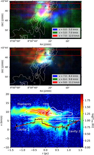
Figure 6. Top: [C ii] RGB map presenting the global kinematic structure of RCW 36 between 0 and 12 km s−1. The color-coding is given in the panel. The white contours indicate the column density  at (1, 2, 4, 8) × 1022 cm−2. The red bar outlines the area of the map used to produce the PV diagram below. The small black vertical line inside the red bar indicates the center (0 pc) for the PV diagram. Middle: same as the top panel, but focusing on the velocity structure in the most redshifted velocity interval between 7 and 11.2 km s−1. Bottom: the [C ii] PV diagram parallel to the bipolar cavities and the 12CO (3–2) emission in white contours (starting at 5 K km s−1 with increments of 10 K km s−1). The solid and dashed red curves, which closely overlap and thus are difficult to separate in this figure, show the fitted functions (second-order polynomial: solid curve; sine function: dashed curve) to the two identified blueshifted expanding [C ii] shells that are found in the two cavities. The black line follows the peak intensity along the expanding shells as a function of radius. At velocities <0 and >12 km s−1, the emission from the high-velocity wings is observed. This emission does not show an elliptical shape in the PV diagram, which would be predicted for expanding shells.
Download figure:
Standard image High-resolution image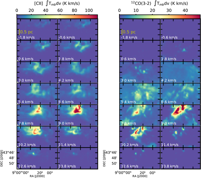
Figure 7. Left: channel maps of [C ii] from −1.8 to 13.8 km s−1 with velocity intervals of 1.2 km s−1 present the velocity structure of RCW 36. Below 6 km s−1, the blueshifted expanding shells are observed in the color map for [C ii]. Right: same as the left panel, but for 12CO (3–2) covering the same area as the [C ii] map. It appears that 12CO (3–2) only marginally traces the expanding shell. At higher velocities, 12CO (3–2) mostly traces the kinematics of the Vela C molecular cloud.
Download figure:
Standard image High-resolution imageTable 1. Minimal Velocity (v
 ) and Corresponding Expansion Velocity (vexp) Obtained for the Two Fitted Functions to the Expanding Shells in the West and the East, Respectively
| Function |
 (km s−1) (km s−1) |
 (km s−1) (km s−1) |
 (km s−1) (km s−1) |
 (km s−1) (km s−1) |
|---|---|---|---|---|
| sine | 1.4 ± 0.1 | 5.1 ± 0.1 ± 0.5 | 0.8 ± 0.9 | 5.7 ± 0.9 ± 0.5 |
| poly | 1.5 ± 0.1 | 5.0 ± 0.1 ± 0.5 | 1.6 ± 0.1 | 4.9 ± 0.1 ± 0.5 |
Note. The fitted functions are a sine function (sine) and a second-order polynomial (poly). The indicated errors for the minimal vLSR correspond to the error on the fit. The two indicated errors for the expansion velocities correspond to the fitting error and uncertainty on the assumed rest vLSR for the shells.
Download table as: ASCIITypeset image
3.3.2. The Kinematics of the Molecular Ring
Our observations also resolve the central molecular ring, which is best visible in the dust column density map and in the 13CO (3–2) emission (Figure 4). However, the ring is also associated with [C ii] emission as shown in the RGB images of Figure 6. The top panel indicates that the eastern part of the ring is more blueshifted than the western part. Since it was proposed, by Minier et al. (2013) and from Figure 1, that the eastern part of the ring is in front of the western part, this velocity structure fits with the proposed expansion of the molecular ring. A zoom into the ring kinematics by the channel maps in Figure 8 confirms this expansion and demonstrates that the expansion is also seen in 13CO (3–2). Unfortunately, it is very difficult to accurately estimate an expansion velocity for the ring. There are several reasons for this: self-absorption effects in all available lines limit an accurate determination of the typical velocity of the gas, stellar feedback breaking through the ring affects the velocity field, and the presence of additional velocity structure in the line of sight (see also A. Bij et al. 2022, in preparation) limits the possibility to use the moment 1 map. Therefore, we estimate the expansion velocity from inspecting the channel maps in Figure 8. The eastern area of the ring is found at 5–6 km s−1, whereas the western part is at ∼8.0–8.8 km s−1. This suggests a typical expansion velocity of 1.0–1.9 km s−1. More generally, Figure 8 shows that [C ii] and CO have the same kinematic structure toward the ring, which implies that they trace the same expansion dynamics. The full ring is thus swept up by the expansion from the cluster with the CO emission at the outer side of the [C ii] emission as would be expected in a PDR structure with internal FUV irradiation. Lastly, in the southwest of the ring, where Figure 4 shows that the integrated [C ii] emission crosses the molecular ring, Figure 8 now shows that 13CO and [C ii] have the same kinematic morphology between 8.0 and 9.6 km s−1.

Figure 8. A zoom-in of the [C ii] channel maps on the ring around the young OB cluster, to focus on the velocity structure in the ring. The overlaid black contours indicate the 13CO (3–2) channel maps at the same velocity starting at 5 K km s−1 with increments of 10 K km s−1. It shows that the kinematics in [C ii] and 13CO (3–2) are very similar toward the ring, unlike the cavities. The eastern part of the ring is already detected starting at 5 km s−1, while the western part of the ring is only detected starting at 7–8 km s−1.
Download figure:
Standard image High-resolution image3.3.3. Filamentary Structures in [C ii]
The PV diagram in Figure 6 also shows significant [C ii] emission around 10 km s−1, with corresponding 12CO (3–2) emission toward the eastern cavity. This emission is indicated with the name "filaments" in the PV diagrams. The typical elliptical signature expected in PV diagrams for expanding shells is not as evident for this [C ii] emission, which could be due to the small velocity difference with the ring (<2–3 km s−1). In the channel maps in Figures 7 and 9, this 10 km s−1 emission displays a filamentary structure that is not typical for expanding shells. However, Figure 9, in particular, also shows that these filaments have a curved morphology that appears to have their origin toward the central cluster. This [C ii] and CO emission might thus originate from low-density filaments, originally converging toward the ridge where RCW 36 formed, which are now being swept away at velocities <3 km s−1 by the feedback from the stellar cluster. Such filamentary gas, which might originally be flowing toward a central filament or ridge, was observed for a wide variety of low- to high-mass star formation regions such as Musca, B211/3, and DR 21 (Goldsmith et al. 2008; Schneider et al. 2010; Palmeirim et al. 2013; Cox et al. 2016; Bonne et al. 2020a). The observed small expansion velocity for these filaments around RCW 36 is quite similar to the expansion velocity in the ring, which suggests that overdensities, which are clearly detected in CO, experience significantly slower expansion driven by stellar feedback. Lastly, no corresponding bright filamentary [C ii] emission at 10 km s−1 is observed toward the western cavity, which might be the result of the molecular cloud morphology around RCW 36 before the onset of stellar feedback.

Figure 9. Channel maps of 12CO (3–2) from 1.0 to 12.4 km s−1 over the full APEX map of RCW 36. The white box indicates the currently observed [C ii] map. Below 4 km s−1, emission in an arc is observed that indicates that the shell is also (weakly) detected in 12CO (3–2). Note the clumpy nature of this 12CO emission originating from the shell. At velocities above 8 km s−1, filamentary gas perpendicular to the central ring is observed.
Download figure:
Standard image High-resolution image3.4. High-velocity Wing Emission
The spectra in Section 3.2 showed the presence of blue- (vLSR < 0 km s−1) and redshifted (vLSR > 14 km s−1) high-velocity [C ii] wings. These high-velocity wings have a brightness up to 5–10 K in individual spectral bins (see Figure 2), which is well above the detection limit for [C ii] with a noise rms of 0.8–1.0 K. In Figure 10 the integrated intensity map of the high-velocity wings shows that the blue- and redshifted wings display a bipolar distribution, similar to what is observed for protostellar outflows in CO (e.g., Bachiller 1996; Arce et al. 2007). However, for RCW 36, there are no known driving protostars or young stellar objects (Ellerbroek et al. 2013a) at the location where the blue- and redshifted outflow wings come together in the plane of the sky. Furthermore, the high-velocity wings are only detected in [C ii]. Even at the high column density ring the wings are at no point detected in 12CO (see spectra C1–C3 in Figure 2), and higher angular resolution observations (A. Bij et al. 2022, in preparation) indicate that there are no protostellar sources in the ring that could drive such powerful mass ejection. The observed [C ii] wings are thus most likely not of protostellar nature.
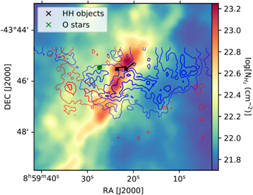
Figure 10. Herschel column density map overlaid with the contours from the integrated blueshifted high-velocity wing (in blue) and the redshifted high-velocity wing (in red) of [C ii]. The location of the two O stars and HH objects, with the orientation of their observed jet (black lines), is also indicated. This shows that the observed high-velocity wings are not associated with the HH jets.
Download figure:
Standard image High-resolution imageIn the currently covered area of RCW 36, there is a significant disparity between the blue- and redshifted integrated wings. Even when integrating over the full 14–22 km s−1 interval, which contains contamination from [13C ii], the redshifted wing remains 2 times less bright and covers a significantly smaller area than the blueshifted wing. These high-velocity wings also do not appear to be directly associated with expanding shells, as they do not show an expanding shell velocity structure in the PV diagram in Figure 6 (i.e., an elliptical velocity profile). The brightest part of the blueshifted wing can be found relatively close to the two reported HH objects in Ellerbroek et al. (2013b). However, Figure 10 also shows the position angle of the HH jets, which indicates that the wings seen in [C ii] are not associated with these HH jets. Lastly, Figure 10 shows that the brightest wings are located around the dense molecular ring and toward the cavity walls. This suggests that the wings might be the result of gas that is entrained from the ring and cavity walls by the impact of feedback processes.
4. Analysis
4.1. The Expanding Shell Energetics from Herschel
Both cavities have blueshifted expanding [C ii] shells. In contrast to the shells in previously studied bubble H ii regions (e.g., Pabst et al. 2020; Luisi et al. 2021; Tiwari et al. 2021), the analysis for RCW 36 is a bit more involved, as it has two expanding cavities and an expanding molecular ring around the cluster. There are two approaches to estimate the expansion energetics. One is based on the Herschel data, and the second one is based on the [C ii] data.
First, we will work with the Herschel data of Vela C. The column density map produced from SED fitting to the 160–500 μm data might not be ideal to calculate the shell mass, as most of these wavelengths particularly trace the cold dust (<20–30 K). Furthermore, the shells in the bipolar cavities are prominent at 160 μm and shorter wavelengths, which could be expected for the strongly irradiated expanding shells if they have a relatively low AV (≲5). In this case, the shell is mostly dominated by the presence of PDRs, which would lead to higher temperatures. A method that would be more sensitive to relatively warm shells was presented in Tiwari et al. (2021), using a column density map produced based on the Herschel 70 and 160 μm map. This makes use of the fact that the optical depth at 160 μm (τ160) can be converted to a hydrogen nucleus column density NH using the dust extinction cross section at this wavelength, which is given by Cext,160/H = 1.9 ×10⁻²⁵ cm2/H (Draine 2003). The optical depth is related to the observed intensity by Iν = Bν (Td )τν , assuming optically thin emission and limited fore/background emission. Bν (Td ) is the Planck function at a specific dust temperature Td . In order to calculate the dust temperature map, the method presented in Peretto et al. (2016) and Bonne et al. (2022), based on the intensity ratio of 70 μm (after smoothing to the resolution of the 160 μm data) and 160 μm, is used. From this dust temperature map, it is then possible to calculate the optical depth and the column density (Draine 2003).
Based on a visual inspection of the Herschel and WISE data at 160 μm and shorter wavelengths, the limb-brightened part of the shell in the cavities corresponds to a width of ∼0.3 pc, which is ∼30% of the 1.0 pc radius for both cavities; see Figure 11. This figure also defines the area of the expanding ring. The estimated masses of the ring and shells are presented in Table 2. To obtain the full mass of the expanding shells in the cavities, the calculated mass in the limb-brightened shells is multiplied by a geometric correction factor of 2.7. This correction factor was calculated using a code that determines the fraction of the shell located in the limb-brightened part of the shell in a 1D cut through the spherical half-shell and then assumes an axial symmetry. Using an expansion velocity of 1.0–1.9 km s−1 for the ring and 5.2 km s−1 for the two expanding shells in the cavities, we then arrive at a total kinetic energy of (2.4–2.6) × 1047 erg; see Table 2.
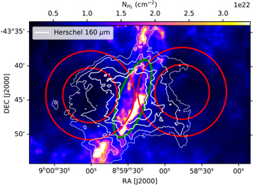
Figure 11. Herschel column density map with overlaid Herschel contours at 160 μm (in white), which is bright toward the ring and cavity walls. In order to calculate the masses for the expansion energetics, the ring is defined by the region encompassed by the green ellipse and the expanding shells in the cavities by the two red annuli. The regions where the annuli overlap with the green ellipse are excluded for the mass calculation of the expanding shells.
Download figure:
Standard image High-resolution imageTable 2. The Mass and the Resulting Kinetic Energy of the Expanding Ring and Shells, Calculated with the Different Methods. This was calculated using EK
=  Mv
Mv .
.
| Region | Mass | Kinetic Energy |
|---|---|---|
| 70 μm and 160 μm Column Density Map | ||
| Ring | 9.1 × 10² M⊙ | (0.9–3.3) × 1046 erg |
| East cavity | 4.5 × 10² M⊙ | (1.2 ± 0.2 ± 0.2) × 1047 erg |
| West cavity | 3.9 × 10² M⊙ | (1.1 ± 0.2 ± 0.2) × 1047 erg |
| Total | (2.4–2.6) × 1047 erg | |
| SED-fitted Column Density Map | ||
| Ring | 4.1 × 10² M⊙ | (0.4–1.5) × 1046 erg |
| East cavity | 2.5 × 10² M⊙ | (6.8 ± 1.3 ± 1.3) × 1046 erg |
| West cavity | 2.3 × 10² M⊙ | (6.2 ± 1.2 ± 1.2) × 1046 erg |
| Total | (1.2–1.4) × 1047 erg | |
| [C ii] Shell | ||
| Full cavity (100 K) | (1.5 ± 0.5) × 102 M⊙ | (4.1 ± 1.4 ± 0.8) × 1046 erg |
| Full cavity (250 K) | (1.1 ± 0.3) × 102 M⊙ | (3.0 ± 1.1 ± 0.6) × 1046 erg |
| Full cavity (500 K) | (1.0 ± 0.3) × 102 M⊙ | (2.7 ± 1.0 ± 0.5) × 1046 erg |
Note. An expansion velocity range of 1–1.9 km s−1 was used for the ring, and an expansion velocity of 5.2 ± 0.5 ± 0.5 km s−1 was assumed for the shells in the cavities. The error on the energy values for the cavity was estimated based on the uncertainty on the expansion velocity. Note that this does not take into account errors on the mass. In the table, "Full cavity" indicates that the eastern and western cavities were not separated. Based on the calculations using different Cul/Aul values, we obtain an uncertainty of 30% on the calculated mass from [C ii].
Download table as: ASCIITypeset image
We note that the expanding central ring contains dust that is also detected at wavelengths >160 μm. When using the mass for the ring from the column density map produced by the SED fitting between 160 and 500 μm, the mass agrees roughly within a factor 2 with the method based on the 160 and 70 μm ratio (i.e., the mass of the ring obtained from SED fitting is about a factor 2 lower; see Table 2). In fact, the results for the bipolar cavities also agree within a factor 2. Identifying the best column density map to calculate the contribution from the central ring is a nontrivial issue, but these results indicate that an uncertainty of at least a factor 2 should be taken into account.
4.2. The Expanding Shell Energetics from [C ii]
[C ii] is a direct tracer of the expanding shells at velocities between 0 and 5 km s−1 in the cavities and can thus be used to calculate its mass and kinetic energy. Note, however, that currently only 50% of the planned region is observed in [C ii]. Therefore, we apply a correction factor to the calculations. The correction factor is calculated by determining the fraction of the 70 μm emission from RCW 36 covered by the current [C ii] map. Using different minimal 70 μm intensities (i.e., 500–1500 MJy sr−1) to define RCW 36, we find that typically 47%–55% of RCW 36 was covered. Therefore, we apply a correction factor of 2.0 ± 0.2. In order to calculate the C+ column densities in the expanding shell, we need the excitation temperature. Generally, this is calculated using the [13C ii] line (e.g., Guevara et al. 2020). However, this is not possible for RCW 36 at the moment because there is no convincing [13C ii] detection corresponding to the emission between 0 and 5 km s−1. Therefore, we calculate the kinetic temperature of the expanding shell from estimating the FUV field strength at the location of the expanding shells and converting this into a C+ kinetic temperature using the PDR Toolbox (Kaufman et al. 2006; Pound & Wolfire 2008). This method is further specified in Appendix C and results in an estimated surface temperature range of 100–500 K, which is a good proxy for the gas temperature that is traced by [C ii] emission and in agreement with work toward other H ii regions (e.g., Schneider et al. 2018; Pabst et al. 2020). Assuming optically thin [C ii] emission for the shell, which is currently justified by the nondetection of [13C ii] emission at velocities lower than 6 km s−1, we use Equation (26) from Goldsmith et al. (2012) to calculate the C+ column density. We assume that [C ii] emission is thermally excited and work with a ratio Cul/Aul = 2 (Cul is the collision rate and Aul the Einstein-coefficient for radiative excitation) because H and H2 number densities are expected to be around (3–6) × 103 cm−3 in the shells. Varying this ratio between 1 and 5, the resulting column density variations remain within 30% at each temperature, which is not significantly larger than other uncertainties such as the temperature (leading to variations up to 50%) or the optically thin assumption. Decreasing the ratio of Einstein coefficients down to Cul/Aul = 0.3 would increase the mass by a factor 2. The column density map for the [C ii] emission between 0 and 5 km s−1 is presented in Figure 12. Integrating the column density map, using the value C/H = 1.6 × 10⁻⁴ from Sofia et al. (2004), the total masses of the expanding shells in the cavities are 1.5 × 10² M⊙, 1.1 × 10² M⊙, and 1.0 × 10² M⊙ at a mean kinetic temperature (Tkin) of 100, 250, and 500 K, respectively. Note that this conversion factor might give a lower limit for the total column density since the expanding shell is also weakly detected in the 12CO (3–2) line and the densities toward the shell of RCW 36 are far higher than the typical densities reported in Sofia et al. (2004), where C/H = 1.6 × 10⁻⁴ is mostly found to be an upper limit for the higher densities in their sample. These uncertainties might be part of the explanation why these masses, and resulting expansion energetics, are significantly lower than the values obtained with the Herschel methods. They are about a factor 4 smaller than the values obtained using the SED-fitted column density map, which gives the lowest values for the Herschel-based calculations. Another reason for this difference might be the spherical assumption when correcting the Herschel limb-brightened shells to a total mass. Recently, Kabanovic et al. (2022) demonstrated with detailed radiative transfer and self-absorption analysis that the expanding shell in RCW 120 is expanding in a flattened, and not a spherical, molecular cloud. A similar point might be valid for the cavities in RCW 36, which would reduce the mass estimated based on the Herschel data.
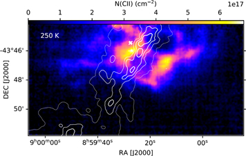
Figure 12. C+ column density map of the blueshifted expanding shells in the cavities, i.e., the [C ii] emission between 0 and 5 km s−1, assuming Tkin = 250 K. When working with a different temperature, the [C ii] column density structure is exactly the same, only with different absolute values. The white contours indicate the Herschel column density, and the white crosses indicate the location of the two O stars.
Download figure:
Standard image High-resolution image4.3. The Mass and Momentum Flux of the High-velocity Wings
At velocities around −8 to 0 km s−1 and 14–22 km s−1 we observe [C ii] emission features that are not associated with expanding shell(s). These blue- and redshifted high-velocity wings rather resemble what is observed for protostellar outflows in CO. However, there are no indications of classical outflow wings in 12CO (3–2) at any location in the map. In addition, [C ii] emission is not a typical tracer for protostellar outflows. Nevertheless, we perform a first-order approximation to calculate the mass and momentum flux of these bipolar [C ii] high-velocity wings using the method presented in Cabrit & Bertout (1992) and Beuther et al. (2002) for bipolar molecular outflows. 14 We first calculate the C+ column density maps associated with the high-velocity wings with the same method used in the previous section for the shells. Again, the resulting C+ mass associated with the wings depends on Tkin and Cul/Aul. Tkin, between 100 and 500 K, is again quite well constrained from the PDR models. Cul/Aul is less constrained, as the density and collision partners of C+ in these high-velocity wings are uncertain. Therefore, taking Cul/Aul ∼ 2 will give a reasonable view on the plausible mass range (within a factor 2). The resulting C+ column density maps of the velocity intervals from −8 to 0 km s−1 (blueshifted wing) and from 14 to 22 km s−1 (redshifted wing) are presented in Figure 13. In the redshifted wing a correction of 1.5 K km s−1 is made to take into account the contribution from the [13C ii] line at velocities above 17 km s−1. Measured with respect to the central velocity of 7 km s−1, these velocity ranges give an observed velocity of 15 km s−1 for both the blue- and redshifted wings, respectively. Since the driving mechanism, and thus the inclination, of the mass ejection is uncertain, we work with an average angle of 57° (Bontemps et al. 1996), which also seems reasonable for mass flows in the cavities that are close to the plane of the sky. From the integrated intensity map of the high-velocity wings, we get a radial extent of 1.5 pc. Taking again into account that currently only half of the cavity is observed, the obtained values are corrected by a factor 2.0 ± 0.2. The resulting mass, mass ejection rate, and momentum flux of the bipolar high-velocity wings, assuming a kinetic temperature of 100–500 K for [C ii], are presented in Table 3.
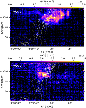
Figure 13. Top: C+ column density map of the blueshifted high-velocity wing between −8 and 0 km s−1, assuming Tkin = 250 K. The white crosses indicate the location of the two O stars. Bottom: same as the top panel, but for the redshifted high-velocity wing between 14 and 22 km s−1.
Download figure:
Standard image High-resolution imageTable 3. The Calculated Mass, Momentum Flux (Fm
), and Mass Ejection Rate ( ) of the Bipolar Wings Observed with [C ii] in the RCW 36 Cavities for Kinetic Temperatures of 100, 250, and 500 K
| Tkin | Mass | Fm |

|
|---|---|---|---|
| 100 K | 4 × 10² M⊙ | 2 × 10⁻² M⊙ km s−1 yr−1 | 7 × 10⁻⁴ M⊙ yr−1 |
| 250 K | 3 × 10² M⊙ | 1 × 10⁻² M⊙ km s−1 yr−1 | 5 × 10⁻⁴ M⊙ yr−1 |
| 500 K | 3 × 10² M⊙ | 1 × 10⁻² M⊙ km s−1 yr−1 | 4 × 10⁻⁴ M⊙ yr−1 |
Note. Based on arguments presented in the text, the errors, which are difficult to quantify for all sources of uncertainty, on these values are easily a factor 2.
Download table as: ASCIITypeset image
5. Chandra
Chandra observations trace the presence of hot plasma formed in the winds of massive stars. A map of diffuse X-ray emission for RCW 36 was presented in Townsley et al. (2014). The methods to extract this diffuse X-ray emission are described in detail in Broos et al. (2010, 2012) and Broos & Townsley (2019). Analyzing the Chandra data will thus allow a more comprehensive view of the feedback processes that are driving the observed dynamics around RCW 36.
5.1. The Diffuse X-Ray Emission Map
The diffuse X-ray emission is presented in Figure 14. The brightest peak is centered on the two O-star candidates of the young cluster. Fainter emission is seen inside the bipolar cavities, which is explained by extinction from the cavity walls when analyzing the X-ray spectra (see Appendix D). The morphology of the diffuse X-ray emission in Figure 14 hints that the hot plasma formed in the OB cluster is leaking out of the H ii region into the ISM beyond the cavities of RCW 36.

Figure 14. Top: diffuse X-ray emission observed with the ACIS instrument on Chandra. The white contours show the 70 μm emission of RCW 36 from Figure 1 starting at 10−1.5 Jy pixel−1 with increments of 0.5 in the exponent. The brightest Chandra emission is centered on the O stars of the cluster, which are indicated by the black cross. In the cavities, there is diffuse emission detected that is significantly weaker than extended emission outside the cavities (outlined by the 70 μm emission). The diffuse emission outside the cavities likely is the result of hot plasma leaking out of the H ii region, which fits with the observed physical connection to the emission inside the H ii region and the fact that the hot plasma fitting blindly converged to very similar properties for the different regions. Two locations where this physical connection is seen are indicated with the red lines. The red box indicates the outline of the currently observed [C ii] map. Bottom: a smoothed image of Chandra/ACIS diffuse X-ray emission in the context of WISE and Herschel images. The five regions used to extract diffuse X-ray spectra are overlaid. The small blue ellipse at field center marks a region excluded from the "Center" diffuse X-ray spectrum because it is dominated by emission from unresolved young stars at the center of the cluster. See Appendix D for details of the X-ray spectral fitting.
Download figure:
Standard image High-resolution imageTo constrain the excitation conditions of the diffuse X-ray emission, X-ray spectra of several regions in RCW 36 are fitted using plasma models in XSPEC (Arnaud 1996). Five diffuse extraction regions, shown in Figure 14, were defined to obtain spectra with sufficient S/N for fitting. X-ray events from hundreds of X-ray point sources were excised from these regions, to minimize their influence on the diffuse X-ray spectra. Details on our methods for fitting diffuse X-ray emission in and around massive star-forming regions are given in Townsley et al. (2019).
The extracted diffuse X-ray spectra and fitting results are presented in Appendix D and Table 8. The central region is filled by a soft, single-temperature thermal plasma plus residual emission from unresolved pre-main-sequence stars in the young cluster. The eastern and western cavities are filled with a thermal plasma of similar temperature. The intrinsic surface brightness of this emission, which corrects for the intervening absorption, is higher than that outside the cavities, confirming that the morphology of the apparent surface brightness map is influenced by intervening absorption. Hot plasma in the ISM surrounding RCW 36 shows two thermal plasma components, one similar in temperature to the RCW 36 emission and one substantially hotter. While the hotter component is likely unrelated background emission (often seen along Galactic plane sight lines), the cooler component is strong evidence that the plasma generated by massive star winds in RCW 36 is leaking out of its H ii region into the surrounding molecular cloud.
5.2. Properties of the Hot Plasma
From the fitted spectra of the hot plasma, the physical properties (plasma density, pressure, etc.) can be calculated with an assumed emissivity curve and a filling factor that was taken to be unity (Townsley et al. 2003). The assumed emissivity curve from Landi & Landini (1999) assumes collisional ionization equilibrium (CIE) for the plasma. This assumption is justified since nonequilibrium effects only become notable below plasma temperatures of 106 K (Vasiliev 2011, 2013), whereas the hot plasma temperature in RCW 36 ((1.7–2) × 106 K) is above this value; see also Table 8. The calculation of the physical properties was not done for the regions outside the bipolar H ii region (north and southeast), as there is no evident assumption for the 3D geometry at these locations. This calculation of the physical properties also was not done for the central region directly around the OB cluster because of the nonequilibrium ionization (NEI) of the plasma and relatively low temperature. As a result, the bandpass correction factor necessary for the limited ACIS bandpass is larger than 40, which would make the results for the center highly uncertain. For the cavities, the bandpass correction factors are 4.4 and 3.4 for the east and west, respectively, which makes their estimated properties less uncertain. The resulting physical properties of the plasma are presented in Table 4. Both cavities have an estimated temperature around 2 × 10⁶ K and electron densities around 0.2 cm−3, which results in an estimated pressure of (0.6–0.9) × 106 K cm−3.
Table 4. Physical Properties of the Diffuse X-Ray Plasma Components for RCW 36, D = 900 pc
| Parameter | Scale Factor | RCW 36 Diffuse Region | |
|---|---|---|---|
| East Bubble | West Bubble | ||
| Observed X-Ray Properties | |||
| kTx (keV) | ⋯ | 0.15 | 0.17 |
| LX,bol (erg s−1) | ⋯ | 4.4 × 1033 | 1.9 × 1033 |
| Vx (cm3) | η | 4.1 × 1056 | 4.1 × 1056 |
| Derived X-Ray Plasma Properties | |||
| Tx (K) | ⋯ | 1.7 × 10⁶ | 2.0 × 10⁶ |
| ne,x (cm−3) | η−1/2 | 0.22 | 0.15 |
| Px /k (K cm−3) | η−1/2 | 0.9 × 10⁶ | 0.6 × 10⁶ |
| Ex (erg) | η1/2 | 7.2 × 1046 | 5.4 × 1046 |
| τcool (Myr) | η1/2 | 0.5 | 0.9 |
| Mx (M⊙) | η1/2 | 0.05 | 0.03 |
Note. Equations detailing how the derived properties were obtained from the observed properties are given in Townsley et al. (2003). The quantity η is a "filling factor," 0 < η < 1, accounting for partial filling of the volume with the X-ray-emitting plasmas. The parameters in the table should be multiplied by the appropriate scale factor (Column (2)) to account for this filling factor. Derived plasma properties are proportional to η1/2 and are thus only weakly sensitive to this correction.
Download table as: ASCIITypeset image
The resulting estimated energy of the plasma in both cavities matches the expansion energy of the expanding shells, presented in Table 2, well (i.e., it is slightly higher than the estimated expansion energy based on [C ii] and slightly lower than the estimates based on Herschel). This suggests that under adiabatic conditions the expanding shells in the cavities might be driven by the hot plasma (e.g., Weaver et al. 1977; Lancaster et al. 2021a). This will be examined in more detail later on, as other processes such as photoionized gas pressure and direct radiation pressure could also play a role. Note that the unity filling factor is an assumption. The appropriate scaling factor (η−1/2, with η the filling factor) to correct for a lower filling factor is also presented in Column (2) of Table 4. This indicates that the resulting plasma properties are not extremely sensitive to the filling factor.
6. Discussion
6.1. 3D Structure of RCW 36
RCW 36 consists of a bipolar cavity and a dense central ring surrounding the waist of the H ii region created by the central OB cluster. In the cavities, the expanding [C ii] shell is only observed at blueshifted velocities, which implies that it is expanding toward us. Fitting the foreground column to the Chandra data toward the cavities, in particular the eastern one, suggests that most column density, observed with Herschel, is associated with and on the near side of RCW 36 from our point of view. The observed [C ii] shells are thus expanding into the predominant nearby column density reservoir of RCW 36. This can offer an explanation why no corresponding redshifted expanding shell is detected for the cavities even though a few expanding filamentary structures are observed toward slightly more redshifted velocities. As most of the column density appears to be located in front, the gas behind the ridge might be mostly diffuse gas. As a result, the hot plasma created by the OB stars would be able to leak from RCW 36 in that direction, as sketched in Figure 15. This is in essence the same scenario observed for RCW 49 in Tiwari et al. (2021). Interestingly, in contrast to RCW 36 (two O-star candidates and ∼1 Myr), RCW 49 contains 37 OB identified stars and is slightly older with an estimated age ∼2 Myr.
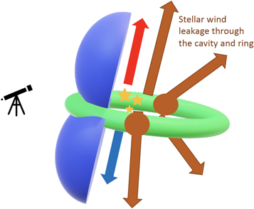
Figure 15. Sketch of RCW 36 seen from the side and indicating our point of view (telescope). With [C ii], we observe blueshifted expanding shells (blue) in the bipolar cavities. The ring (green) is expanding at a lower velocity into the Vela C molecular cloud. The blue and red arrows indicate the high-velocity mass ejection in the cavities associated with the wings (blue and red) in the spectra. The brown arrows indicate the hot plasma leakage, which is presumably most effective toward the back of RCW 36, where no redshifted expanding shells are observed with the [C ii] data, but we also observed that it can channel through punctures in the ring (brown patches on the ring).
Download figure:
Standard image High-resolution imageTo obtain a first idea of the expansion timescale for the dense molecular ring, we use the estimated expansion velocity between 1.0 and 1.9 km s−1 and an estimated radius of 0.9 pc. As it is unclear what drives the expansion of the ring, we calculated the Spitzer expansion timescale for expansion driven by ionizing radiation (Spitzer 1978), the Weaver solution for expansion driven by stellar winds (Weaver et al. 1977), and the ballistic expansion timescale that can be expected if shell expansion is driven by stellar winds in an isothermal density field with a power-law index of −2 (Geen & de Koter 2022). The Spitzer solution gives an expansion timescale of 1.2–1.7 Myr, the Weaver solution gives a timescale of 0.3–0.6 Myr, and the ballistic expansion gives a timescale of 0.5–0.9 Myr. The calculations of the Spitzer and Weaver solutions are further specified in Appendix F. Broadly speaking, the Spitzer and ballistic solutions for the dense ring appear to be in better agreement with the cluster age than the Weaver solution (Ellerbroek et al. 2013a). However, the upper value of the Spitzer solution, which might be the most representative one (see Appendix F), has an equally large deviation from the estimated cluster age as the Weaver solution. The cavities, on the other hand, have a radius of ∼1.0 pc and an expansion velocity of 5.2 ± 0.5 ± 0.5 km s−1, which results in an estimated Spitzer expansion timescale of 0.2–0.4 Myr (see Appendix F), a Weaver expansion timescale of 0.1 Myr, and a ballistic expansion timescale of ∼0.2 Myr. This is roughly a factor 3–5 shorter than for the ring and suggests that the expansion in the cavities is a recent feature. Note that this assumes that the cavity expands from the center of the cavity, which might not be fully correct. Considering that the expansion starts from the center of RCW 36, we get a radius in the range of 1.5–2.0 pc. This results in an estimated ballistic expansion timescale of 0.3–0.4 Myr, which is still shorter than the expansion of the dense ring. RCW 36 thus shows inhomogeneous expansion: relatively slow expansion in the dense gas, followed by increasing expansion velocity once the expansion reaches the lower-density gas. This fits with relatively low (<3 km s−1) expansion velocity of the denser filamentary structures perpendicular to the ring.
Samal et al. (2018) noted that only 16 of the 1377 H ii regions considered in their sample are visibly identified as bipolar H ii regions. A correction factor has to be taken into account based on inclination selection effects, but, as mentioned in Samal et al. (2018), this still implies that bipolar H ii regions are rather rare. From the faster expansion in the bipolar cavities of RCW 36 compared to the ring, it can be argued that the morphology of RCW 36 is changing rapidly (on ∼0.2 Myr timescales) and thus that a H ii region might only be observed as bipolar for a part of its evolution. As a short exercise, assuming a correction factor 5 for the inclination 15 and a potential correction factor 5 for the short timescale 16 would imply that up to 30% of the H ii regions might go through a bipolar phase. However, this remains speculative at the moment since this is based on a single case. More generally, the observation of expanding half-shells, instead of fully spherical shells, in [C ii] emission toward H ii regions (e.g., Anderson et al. 2019; Pabst et al. 2020; Luisi et al. 2021; Tiwari et al. 2021) and the evidence of important hot plasma leakage can fit in the view of the ISM where (massive) stars form in a complex organization of filaments and sheets. The creation of bipolar H ii regions can then occur when an O star forms close to the midplane of a sheet-like structure such that the radiation and wind break out on both sides at about the same time. The hot plasma can then start driving expanding shells in the lower-density gas outside the sheet. This is, however, speculative since it is based on a single case, while the observations also indicate that the expansion strongly depends on the density structure. Furthermore, simulations by Wareing et al. (2017) suggest that the bipolar morphology remains present for a significant part of their simulation. This is due to the apparent low expansion velocity (<1 km s−1) for the cavities in their simulation, which is not in agreement with the observed velocities in the cavities for RCW 36. As the expansion dynamics might vary from region to region, a detailed analysis of age and dynamics of a sample of bipolar H ii regions will be required to fully address this question.
6.2. The Pressure and Energy Budget in RCW 36
Analysis of the Chandra data shows that a hot plasma, created by the stellar winds, pervades RCW 36 and that it has the required energy to drive the observed expanding shells in both cavities. To discuss the role of different physical processes, the associated pressure terms were estimated and are presented in Table 5. Specific assumptions made for these calculations are specified in Appendix E. The thermal pressure from the hot plasma in both cavities is ∼(0.6–1.0) ×106 K cm−3, which is slightly larger than the estimated thermal pressure of the photoionized gas, i.e., (4.6–5.0) × 105 K cm−3, derived from the SHASSA Hα observations (Gaustad et al. 2001). However, as for the hot plasma, if the photoionized gas is confined in a subregion of the cavities, this will increase the estimated pressure. As a result, these terms probably dominate over the direct radiation pressure in the cavities; see Table 5. Since cavities are filled by both the hot plasma and photoionized gas, the photoionized and collisionally ionized gas can thus be in pressure equilibrium across the contact discontinuity.
Table 5. The Estimated Pressure (Range) for the Different Components Associated with the Expanding Shells in the Cavities and the Dense Molecular Ring around the Central Cluster
| Pth/k (K cm−3) | Prad (K cm−3) | Pturb/k (K cm−3) | PB /k (K cm−3) | Pram/k (K cm−3) a | |
|---|---|---|---|---|---|
| Bipolar Cavities | |||||
| Hot plasma | (0.6–0.9) × 106 | ||||
| H ii region | (4.6–5.0) × 105 | 4.5 × 10⁵ | |||
| Ambient cloud | (0.5–2.5) × 104 | <(1.3–6.7) × 105 | (0.3–1.4) × 105 | (0.7–3.5) × 106 | |
| Shell (internal) | (2.5–7.5) × 105 | (0.5–1.7) × 106 | <(0.8–3.8) × 105 | ||
| Center + Dense Ring | |||||
| Hot plasma | |||||
| H ii region | 2 × 10⁶ b | 1.2 × 10⁶ | |||
| Ambient cloud | (0.2–2.0) × 105 | <(1.3–13) × 106 | (0.4–7.8) × 106 | (0.3–2.8) × 106 | |
| Ring (internal) | (2.4–3.6) × 105 | (3.0–3.7) × 106 | |||
Notes. The calculation of the values is presented in more detail in Appendix E.
a Ram pressure provided by the ambient cloud on the expanding shell/ring. b Minier et al. (2013).Download table as: ASCIITypeset image
The physical processes that drive expanding motion of H ii regions are still a matter of debate. Simulations generally predict that ionizing radiation is the main driver of expansion compared to stellar winds (e.g., Haid et al. 2018; Geen et al. 2021; Ali et al. 2022). Yet simulating the high dynamic range of temperatures and densities associated with the presence of stellar winds in the ISM is challenging (e.g., Dale 2015). Observations by Lopez et al. (2014) also indicate that the ionized gas pressures appear to dominate most H ii regions; however, other observational studies (e.g., Pabst et al. 2019; Luisi et al. 2021; Tiwari et al. 2021) have proposed that stellar winds drive the high-velocity expansion detected with spectrally resolved [C ii] observations. Above we already noted that thermal pressure of the ionized gas and hot plasma seem to be of the same order for RCW 36. Here, we will discuss the associated energy terms. Based on the SHASSA Hα intensity, the ionizing photon flux in each cavity is ∼8.5 ×1046 s−1; see Appendix E. This results in a total injected energy of ∼6.2 × 1049 erg over the estimated lifetime of the cluster (i.e., 1.1 Myr) when assuming an energy of 13.6 eV for the ionizing photons. Taking into account that the coupling efficiency of ionizing radiation energy to radial expansion typically is <10−4 (Haid et al. 2018), this is about an order of magnitude too small to explain the expanding motion of the shells in the cavities. We do note that at very early evolutionary stages in Haid et al. (2018) the coupling efficiency for ionizing photons is significantly higher. However, considering a coupling efficiency of 10−3 over the first 0.3 Myr remains insufficient to explain the observed expansion. Therefore, unless the coupling efficiency for ionizing photons in Haid et al. (2018) is about an order of magnitude lower than in RCW 36, we propose that the hot plasma created by stellar winds drives the expansion of the blueshifted shells in the cavities.
On the other side of the shell, ram pressure, thermal pressure, and magnetic pressure from the ambient cloud confine the shell. The values in Table 5 indicate that in this low-density region the ram pressure confines the shell. Inside the compressed shell, turbulent pressure seems to be the dominant term to prevent the shell from being further compressed between the hot plasma on one side and ram pressure on the other side. Even though the estimated magnetic pressure in the shell is significantly smaller than the turbulent pressure, it might play a role in limiting the initial compression rate of the propagating shock that is driven by the expansion. Inspecting the BLASTPol magnetic field map toward RCW 36 in Figure 16, it is observed that the magnetic field morphology follows the bipolar cavities and forms a kink near the ring where the polarization fraction drops. This behavior where the magnetic field orientation is aligned with the shell morphology around a H ii region, as it is dragged along by the expansion, was recently also observed in the Keyhole Nebula (Seo et al. 2021) and NGC 6334 (Arzoumanian et al. 2021). The magnetic field morphology in the ring and whether it significantly affects the expansion remain unclear with current data. This requires higher angular resolution observations (A. Bij et al. 2022, in preparation). In the ring, it is also unclear which process (ionizing radiation or the hot plasma) drives the expansion. The number of ionizing photons and coupling efficiency is sufficient to drive the ring expansion, but the hot plasma in the ring remains unconstrained. As a result, we cannot reach a firm conclusion.
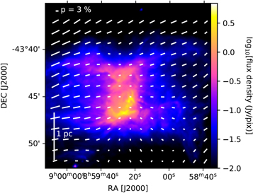
Figure 16. Herschel 70 μm map of RCW 36 overlaid with the magnetic field orientation obtained from BLASTPol at 500 μm (Fissel et al. 2016, 2019). The magnetic field orientation tends to follow the edges of the shells and associated kink near the central ring. It is also observed that the polarization fraction quickly drops toward the central ring, which might be associated with the complex morphology in this region that remains unresolved with the BLASTPol data.
Download figure:
Standard image High-resolution image6.3. Feedback-driven Turbulence
In Figure 17, a noteworthy increase in 13CO (3–2) velocity dispersion is observed in the ring of RCW 36 compared to the surrounding regions of the Vela C molecular ridge, which does not seem to be explained by opacity broadening; see Appendix E. This indicates that the mechanical energy input from stellar feedback can significantly increase the turbulent energy in the compressed gas. This energy injection might thus play a role in setting the thickness of the shell, as it provides a rough pressure equilibrium with both sides of the shell. Specifically, the turbulent pressure in the ring, derived from the spectral line width, is similar to or higher than the ram pressure provided by the ambient gas; see Table 5. Otherwise, the shell would be further compressed until an increased temperature (or magnetic field strength or turbulence) due to this compression would halt it. From the information provided by the 13CO (2–1) line width, corrected for optically thick line broadening (Appendix E), it is possible to estimate the turbulence injection by stellar feedback in the molecular ring. The calculated total turbulent energy injection in the ring and cavity shells is given in Table 6. From Figure 17, it is reasonable to assume a line width for this gas of 0.7 km s−1 before the onset of stellar feedback, which would give a total turbulent energy of 2.5 × 10² M⊙ (km s−1)2 for the gas now located in the ring. Comparing this with the value for the ring in Table 6, this implies that the turbulent energy of the gas, after opacity broadening correction, has roughly increased by more than 60% compared to the onset of stellar feedback. Turbulence typically dissipates over a few crossing timescales (tcross = d/σlos; Ostriker et al. 2001). For the ring, with a width of ∼0.1 pc, this gives a crossing timescale of 1.1 × 10⁻¹ Myr. Using this timescale results in a turbulence dissipation rate of 2.4 × 1033 erg s−1 that has to be injected to maintain the turbulent line width. This is only a small fraction of the probable energy injection rate by the O-star candidates, which will be discussed in more detail in the next section.
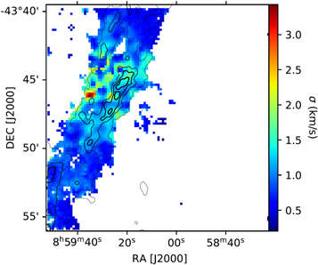
Figure 17. The velocity dispersion map of 13CO (3–2) for RCW 36. The contours indicate the Herschel column density map. Despite the relatively limited extent of the map, it becomes clear that there is a significant velocity dispersion increase at the ring surrounding the OB cluster.
Download figure:
Standard image High-resolution imageTable 6. The Turbulent Energy (Eturb), Dissipation Timescale (tdiss), Turbulent Dissipation Rate  , and Total Injected Turbulent Energy (Eturb,tot) for the Dense Ring and the Full Expanding Shell Associated with the Bipolar Cavities
| Eturb (erg) | tdiss (Myr) |
 (erg s−1) (erg s−1) | Eturb,tot (erg) | |
|---|---|---|---|---|
| Ring | 8.2 × 1045 | 1.1 × 10⁻¹ | 2.4 × 1033 | 8.2 × 1046 (over 1.1 Myr) |
| Shells (from [C ii]) | 2.2 × 1046 | 2.0 × 10⁻¹ | 3.2 × 1033 | 2.2 × 1046 (over 0.2 Myr) |
Note. These calculations for the shell make use of the typical velocity dispersion of 1.5 km s−1 in the expanding shell and the shell mass deduced from [C ii].
Download table as: ASCIITypeset image
6.4. Leakage of the Hot Plasma
In Section 5.1 we proposed that there is leakage of the hot plasma through the diffuse medium around RCW 36, which leads to the hot plasma found outside RCW 36 in Figure 14. To quantify the leakage, we have to estimate the total energy injected in the ISM by the stellar winds of the OB cluster. This is done using several stellar atmosphere models, as there is a large uncertainty on the actual stellar wind mass-loss rates, which from observations appear to be lower than predicted by the standard models (e.g., Martins et al. 2004, 2005b; de Almeida et al. 2019). However, recently it was proposed that the observed values are underestimated because observations miss a significant part of the stellar winds, as a large fraction of the stellar wind might be in a hot phase that is not traced by the observations (Lagae et al. 2021). To cover the range of possibilities, we will use the relations that were put forward in Equation (12) of Vink et al. (2000), Equation (3) of Lucy (2010), Equation (11) of Krtička & Kubát (2017), and Equation (20) of Björklund et al. (2021), all with a terminal velocity of 2500 km s−1 (e.g., Lamers et al. 1995; Krtička & Kubát 2017; Lagae et al. 2021). The formulae differ in the choice of critical parameters and their dependencies (luminosity, metallicity, effective temperature, terminal velocity, etc.), but it is beyond the scope of this paper to discuss their differences in more detail. In any case, employing a range of relations allows us to cover the standard predicted mass ejection rate from stellar models (Vink et al. 2000) to predictions that are more adapted to fit with the current observations (Björklund et al. 2021). For the 09V and 09.5V star candidates in the cluster we use the stellar parameters from Martins et al. (2005a) and Pecaut & Mamajek (2013) to take into account the effects of different stellar models. The results are summarized in Table 7, which indicates a significant change depending on the stellar model used and an even larger effect related to the stellar wind mass-loss rate prescription used. Only taking into account the two O-star candidates of RCW 36, this results in a total injected energy in the range of 4.7 × 1047 erg to 8.3 × 1048 erg over 1.1 Myr; see Table 7. This order-of-magnitude difference depending on the model might be overcome by the missing hot phase proposed in Lagae et al. (2021); however, future observations will have to address whether there is indeed such a large fraction of the stellar winds in the hot phase. The energy in the hot plasma of RCW 36, from Table 4, is of the order of (1–2) × 1047 erg, implying that >50%, and potentially up to 97%, of the total injected stellar wind energy is no longer found in the hot plasma.
Table 7. The Stellar Wind Mass Ejection Rates ( ) and Total Ejected Stellar Wind Energy (ESW)
| Vink et al. (2000) | Lucy (2010) | Krtička & Kubát (2017) | Björklund et al. (2021) | ||
|---|---|---|---|---|---|
| Model | Star | log[ (M⊙ yr−1)] (M⊙ yr−1)] | log[ (M⊙ yr−1)] (M⊙ yr−1)] | log[ (M⊙ yr−1)] (M⊙ yr−1)] | log[ (M⊙ yr−1)] (M⊙ yr−1)] |
| Martins et al. (2005a) | O9V | −7.35 | −8.56 | −7.78 | −8.31 |
| Martins et al. (2005a) | O9.5V | −7.57 | −9.00 | −7.94 | −8.53 |
| Pecaut & Mamajek (2013) | O9V | −7.12 | −8.56 | −7.61 | −8.10 |
| Pecaut & Mamajek (2013) | O9.5V | −7.35 | −8.58 | −7.78 | −8.31 |
| ESW (erg) | ESW (erg) | ESW (erg) | ESW (erg) | ||
| Martins et al. (2005a) | O9V | 2.7 × 1048 | 1.7 × 1047 | 1.0 × 1048 | 3.0 × 1047 |
| Martins et al. (2005a) | O9.5V | 1.6 × 1048 | 5.7 × 1046 | 6.7 × 1047 | 1.7 × 1047 |
| Martins et al. (2005a) | total | 4.3 × 1048 | 2.3 × 1047 | 1.7 × 1048 | 4.7 × 1047 |
| Pecaut & Mamajek (2013) | O9V | 5.4 × 1048 | 1.9 × 1047 | 1.7 × 1048 | 5.4 × 1047 |
| Pecaut & Mamajek (2013) | O9.5V | 2.9 × 1048 | 1.7 × 1047 | 1.1 × 1048 | 3.1 × 1047 |
| Pecaut & Mamajek (2013) | total | 8.3 × 1048 | 3.6 × 1047 | 2.8 × 1048 | 8.5 × 1047 |
Note. Bottom: the resulting total ejected energy over the lifetime of the cluster is calculated assuming an age of 1.1 Myr and using a terminal wind velocity of 2500 km s−1.
Download table as: ASCIITypeset image
Stellar wind energy-loss methods were listed in Townsley et al. (2003), Harper-Clark & Murray (2009), and Rosen et al. (2014). Here we will explore the options. From Table 4, it is found that the hot plasma luminosity is a factor 3 to more than an order of magnitude lower than required to explain the missing energy in the hot plasma. The injected turbulent energy in the molecular ring, presented in Table 6, is a factor 5 to two orders of magnitude smaller than the total injected energy as well. Thermal conduction at the interface of the hot plasma and the turbulent shell layer is another potential way to lose the plasma energy. Recently, work by Lancaster et al. (2021a, 2021b) indicated that cooling can be very efficient at the interface because of turbulent substructure and that this could even explain all the observed missing hot plasma energy. However, it was also noted that thermal conduction is strongly reduced when a (weak) magnetic field is parallel to the shell (Soker 1994; Rosen et al. 2014). This is the case for RCW 36 based on Figure 16, and it should be noted that Lancaster et al. (2021a, 2021b) currently do not include the magnetic field. Simulations in Arthur et al. (2011) indicate that the magnetic field will be mostly perpendicular to the shell in the ionized gas and aligned with the shell in the neutral gas. Rosen et al. (2014) note that a parallel magnetic field with 1 μG would decrease the thermal conduction by several orders of magnitude. In RCW 36, a magnetic field strength of at least several μG is expected (Crutcher 2012), which seems to exclude thermal conduction based on this work. However, more in-depth theoretical studies of energy loss at the turbulent interface, including the magnetic field, would be invaluable to better constrain this. Lastly, wind energy transfer to dust grains through collisions was also excluded in Rosen et al. (2014) as a plausible explanation. This suggests that the majority of the stellar wind energy might have leaked through lower-density regions out of RCW 36. Therefore, we here try to estimate the plasma energy leakage from RCW 36 based on Equation (8) from Harper-Clark & Murray (2009). As we propose that the region is fully open, at one side of the region we use a shell cover fraction (Cf ) of 0.5 for RCW 36 and a radius of 1 pc. Plugging in these values with the hot plasma parameters from Table 4 gives a current energy leakage per cavity of −2.0 × 1035 erg s−1, which is almost two orders of magnitude larger than derived values from other processes in this work. Since leakage probably occurred over the evolution of the H ii region, we use an intermediate radius of 0.5 pc to estimate the leakage over the lifetime of RCW 36. Note that this is only an approximation, as we have no detailed information on the time evolution of RCW 36. It should also be noted that the Cf definition in Harper-Clark & Murray (2009) assumes equal leakage in all directions, whereas in RCW 36 we propose that leakage has a preferential direction. This then gives a total leaked plasma energy of −1.7 × 1048 erg over 1.1 Myr. Compared to the values in Table 7, this suggests that leakage indeed has the potential to account for most missing hot plasma energy.
If there is indeed such strong hot plasma leakage, it could be wondered whether the leaking plasma still has an effect on the molecular cloud. Studying the large-scale molecular cloud structure around RCW 36 with sensitive dust continuum observations (i.e., Herschel and BLASTPol), it can be noted that RCW 36 is located at the center of a large, low column density region in Vela C (Hill et al. 2011; Fissel et al. 2016); see Figure 18. Furthermore, inspecting Figure 18, we observe that the leaking hot plasma shows hints that it correlates with the structure of this large, low column density region. It is thus possible that the potential large fraction of leaking hot plasma clears the low-density ambient cloud on a larger scale. When the injected feedback energy escapes into the diffuse ISM through such lower-density regions or "chimneys" in the cloud, it can thus further disrupt these regions and their mass provision to the ridge around RCW 36. From the large-scale SHASSA Hα map presented in Figure 19, we confirm that this low-density region is indeed a channel of feedback energy leaking into the larger cloud. Estimating the number of photons in these larger cavities is relatively uncertain, as their extent is not strongly constrained. Excluding the Hα emission in the cavities defined by the 70 μm emission, we obtain ionizing photon fluxes as high as (6–7) × 1046 s−1 in these larger cavities. This is fairly similar to the values obtained inside the 70 μm cavities and thus supports significant leakage from RCW 36 into the diffuse cloud.

Figure 18. Herschel column density map of the region in Vela C around RCW 36 (outlined by the green 70 μm contour). The bipolar cavity only fills up a part of the large, low column density region around RCW 36, indicated by the dashed white circles. The black to orange contours indicate the increasing diffuse Chandra X-ray emission. This shows some hints of a correlation between the diffuse X-ray emission and the column density structure in the larger, low-density regions surrounding RCW 36, e.g., in the north and southeast of the map. The red box indicates the region covered by the Chandra data.
Download figure:
Standard image High-resolution image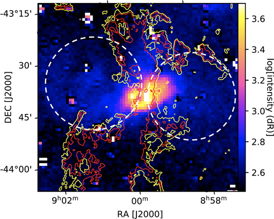
Figure 19. SHASSA Hα map of the larger region around RCW 36. The peak Hα emission corresponds to the center of RCW 36. The yellow and red contours indicated the Herschel column density contours at  = 4 × 1021 cm−2 and 6 × 1021 cm−2, respectively. The white dashed circles indicate the same large-scale low-density cavities as in Figure 18. These cavities are clearly emitting Hα emission, associated with the leakage of ionizing photons, compared to unperturbed regions in the Vela C molecular cloud.
Download figure:
Standard image High-resolution imageAs Vela C still is a relatively young molecular cloud where RCW 36 is the first H ii region, this suggests that the leakage is the result of the molecular cloud morphology before feedback sets in. This presence of lower-density gas (or voids) is expected if molecular clouds are indeed built out of filaments and sheets.
6.5. The Implication of the High-velocity [C ii] Wings
The bipolar wings at high velocities in [C ii] show no clear expanding shell morphology and are not driven by protostars in the ring, but rather by feedback from the OB cluster. This could explain why the wings become less clear at the high column density region of the ring in Figure 10. [C ii] high-velocity wings were also found in the bipolar regions S106 (Simon et al. 2012) and NGC 7538 IRS1 (Sandell et al. 2020). Unlike S106 (Schneider et al. 2018), [O i] is not clearly detected in the wings of RCW 36, which suggests that the density in these wings is comparatively low. In NGC 7538 IRS1, the wings are also detected in 12CO (3–2), which suggests that for NGC 7538 IRS1 the [C ii] wings might trace a protostellar outflow there.
To investigate whether ablation by stellar winds can drive the mass ejection observed with the [C ii] wings, we compare the energy (and momentum) rates for the stellar winds and the [C ii] wings. The energy injection rate of the most favorable stellar wind models (∼(3.9–7.5) × 1042 erg yr−1, from Vink et al. 2000) is of the same order as the outflow energy rate seen with the [C ii] wings (∼(3–5) × 1042 erg yr−1). As the [C ii] outflow parameters should be accurate within a factor 2–3 according to our evaluation in Section 4.3, this suggests that stellar wind ablation might be able to continuously drive the observed [C ii] wings. If these high-velocity wings are continuously ejected from RCW 36, it might account for a significant fraction of the missing plasma energy. However, it has to be taken into account that we also observe actual leakage of the hot plasma and that there are other potential stellar wind energy sinks discussed in previous sections. In addition, this conclusion is only valid for the Vink et al. (2000) models. The estimated energy injection rate by all other models would not be able to explain the observed wings. When considering the total momentum injection rate of the stellar winds, this is about two orders of magnitude lower than the momentum flux observed for the [C ii] wings.
Another potential driver would be the radiation from the OB cluster. In the simulations by Kim et al. (2018), which focus on radiation feedback in molecular clouds, they found mass ejection with velocities between ∼6 and 40 km s−1 as a result of thermal and radiation pressure from ionizing radiation. Radiation might thus be able to drive the observed mass ejection from the center of RCW 36. The calculated radiation pressure (I/c) at r = 0.9 pc (corresponding to the ring) is 1.2 × 10⁶ K cm−3 and thus not significantly higher than the pressure from the hot plasma in the cavities. If the acceleration originates in the ionized gas closer to the OB cluster, the radiation pressure would be higher and could thus more easily drive high-velocity mass ejection into the low-density cavities. As the ionized gas does not cover the full region, because of the hot plasma, this also increases the thermal pressure of the ionized gas. However, there is very little mass inside the central ring (Minier et al. 2013), which implies that the mass ejection should happen at the surface of the ring and/or bipolar cavities. The mass ejection seen with the wings might thus be driven by a combination of stellar wind and pressure from the ionizing radiation. This combination would leave more room for the observed hot plasma leakage and other energy sinks. In general, it thus remains challenging to explain the observed wings with the constrained feedback mechanisms for RCW 36.
The mass ejection rate derived from the [C ii] wings in Table 3 is high. It suggests that (4.8–7.4) × 102
M⊙ can be removed from the region confined by the ring in RCW 36 over the current lifetime of the OB cluster (or (0.9–1.3) × 102
M⊙ over 0.2 Myr). This could have important implications for the star formation efficiency (SFE) in the cloud. If this mass ejection is going on for 1.1 Myr, which could fit with the missing hot plasma energy, it would have already removed about the same mass from the original star-forming region as what is now found in the molecular ring and more than an order of magnitude more than the ∼20 M⊙ of ionized gas confined by the ring (Minier et al. 2013). We found no indications of inflow toward RCW 36 from the ambient gas, as it is actively being swept away, so the main mass inflow would happen along the ridge of Vela C. Using πR2
 , it is then possible to calculate the remaining mass inflow to the RCW 36 ring through the ridge, where R is the radius, vinf the inflow velocity, and ρ the density. Here we assume that the 1.5 km s−1 velocity gradient along RCW 36 (Fissel et al. 2019) is associated with inflow, though it is equally plausible that this is mainly the result of expansion. This gives
  = 0.7 × 10⁻⁴
M⊙ yr−1 when we further assume R = 0.1 pc (Minier et al. 2013) and
= 0.7 × 10⁻⁴
M⊙ yr−1 when we further assume R = 0.1 pc (Minier et al. 2013) and  = 2.4 × 104 cm−3 (converted to the density assuming a mean molecular mass μ = 2.33). The inflow rate is thus more than a factor 5 lower than the mass ejected from RCW 36 and therefore has a small effect on the disruption. The observed mass ejection rate could thus stop any new star formation around RCW 36 on the timescale of 1–2 Myr.
It is also interesting that the mass ejection rate is within a factor two of the typical proposed mass inflow rates (∼10−3 M⊙ yr−1) in globally collapsing hubs and ridges before massive stars have formed (e.g., Schneider et al. 2010; Peretto et al. 2013). This implies that the observed mass ejection can remove the mass from the central region on roughly the same timescale that the collapsing hub/ridge provides mass inflow (i.e., a few freefall timescales of the hub), which is consistent with several simulations that emphasize the importance of stellar feedback to maintain a low SFE in molecular clouds (e.g., Dale et al. 2012; Walch et al. 2012). The observations of RCW 36 thus suggest that stellar feedback is essential in preserving the low SFE in proposed dynamic high-mass star-forming scenarios owing to effective mass removal from the originally collapsing parsec-scale region.
There are still several uncertainties related to this rapid mass removal (when the high-velocity mass removal started exactly, the currently incomplete map, etc.), but future studies using the larger statistical sample that will be provided by the FEEDBACK Legacy program will give further insight into the timescale of this rapid mass removal and how it affects the SFE in high-mass star-forming regions.
7. Conclusions
We presented the currently obtained [C ii] and [O i] observations from the SOFIA FEEDBACK Legacy program toward RCW 36, a bipolar H ii region in the young Vela C molecular cloud. These observations are complemented with 12CO (3–2) and 13CO (3–2) observations from APEX, Chandra X-ray observations, Herschel photometric data, and the BLASTpol dust polarization observation at 500 μm. The main results can be listed as follows:
- 1.The [C ii] and 13CO (3–2) data show that the central molecular ring is expanding with an estimated velocity of 1.0–1.9 km s−1 (see Section 3.3.2).
- 2.The [C ii] and 12CO (3–2) data show the presence of several filaments in the ambient cloud that are being swept away with velocities <3 km s−1 (see Section 3.3.3).
- 3.The [C ii] line unveils blueshifted expanding shells in the bipolar cavities with a velocity of ∼5.2 ± 0.5 ± 0.5 km s−1 (see Section 3.3.1).
- 4.The [C ii], [O i], and 12CO (3–2) spectra have important absorption signatures toward the bright molecular ring (see Section 3.2).
- 5.The [C ii] emission indicates that the warm gas from the PDR layer has broken through the dense swept-up ring in the southwest of this ring (see Section 3.3.2).
- 6.The BLASTPol data show that the magnetic field, dragged along by the expansion, follows the curvature of the shells around the bipolar cavities. However, the magnetic field orientation might have set the direction of the bipolar cavities. Higher-resolution observations are needed to address this (see Section 6.2).
- 7.The 13CO (3–2) emission has an increased line width in the swept-up ring compared to the unaffected ridge in Vela C, which might alter the outcome of the second generation of star formation toward RCW 36 (see Section 6.3).
- 8.Diffuse Chandra emission traces a hot plasma, created by stellar winds, that fills RCW 36 and appears to be able to drive the 5.2 km s−1 blueshifted expanding shells in the cavities (see Section 5).
- 9.Fitting the Chandra data also demonstrates that the observed hot plasma outside the H ii region is likely hot plasma leaking from the H ii region.
- 10.We find that between 50% and 97%, depending on the stellar wind model, of the injected stellar wind energy is missing in RCW 36. Hot plasma leakage can provide a consistent explanation for this, but we cannot fully constrain the contribution from energy sinks at the hot plasma−shell interface (see Section 6.4).
- 11.We showed that the hot plasma and ionizing photon leakage has cleared a larger region around RCW 36 in the Vela C molecular cloud (see Section 6.4).
- 12.The [C ii] spectra have bipolar high-velocity wings in the cavities without a visible expanding shell velocity structure, nor a counterpart in CO. These wings trace high-velocity (v > 15 km s−1) and effective (∼5 × 10⁻⁴ M⊙ yr−1) mass ejection from RCW 36 (see Section 6.5).
The observed rapid shell expansion in the cavities compared to the ring indicates that the expansion accelerates when it reaches lower-density gas. This suggests that this clear bipolar stage might only be a relatively short phase in the evolution of RCW 36 and thus even that a bipolar morphology at some point in expanding H ii regions might be more common than previously thought. The observed multistage expansion morphology, as well as the proposed important leakage, points to a scenario where stellar feedback evolves in a structure of filaments, sheets, and lower-density ambient gas that make up the Vela C molecular cloud. Lastly, the expansion timescale of the ring and rapid mass ejection indicate that stellar feedback can rapidly suppress local massive star formation in a cloud (in 1−2 Myr). This could even allow to maintain a low SFR in gravitationally collapsing regions of a molecular cloud where massive stars form. Additionally, the proposed clearing of the ambient low-density cloud can prevent further provision of cold gas necessary to continue high-mass star formation.
We thank the anonymous referee for detailed and very insightful comments that significantly improved the quality of this paper. We thank F. Martins and J.-C. Bouret for providing comments on the modeling and observations of stellar winds related to this work. We thank F. Comeron for fruitful discussions on the interpretation of the star cluster observations toward RCW 36. We further thank M. Pound and M. Wolfire for discussions related to PDR structure and the PDR Toolbox.
This work is based on observations made with the NASA/DLR Stratospheric Observatory for Infrared Astronomy (SOFIA). SOFIA is jointly operated by the Universities Space Research Association, Inc. (USRA), under NASA contract NNA17BF53C, and the Deutsches SOFIA Institut (DSI) under DLR contract 50 OK 0901 to the University of Stuttgart.
We thank the USRA and NASA staff of the Armstrong Flight Research Center in Palmdale and of the Ames Research Center in Mountain View, as well as the Deutsches SOFIA Institut for their work on the observatory. We acknowledge the support by the upGREAT team for operating the instrument, for planning the detailed observing scenarios, and in the calibration of the data. The development and operation of upGREAT were financed by resources from the MPI für Radioastronomie, Bonn, from Universität zu Köln, and from the DLR Institut für Optische Sensorsysteme, Berlin, and by the Deutsche Forschungsgemeinschaft (DFG) within the grant for the Collaborative Research Center 956, as well as by the Federal Ministry of Economics and Energy (BMWI) via the German Space Agency (DLR) under grants 50 OK 1102, 50 OK 1103, and 50 OK 1104.
The FEEDBACK project is supported by the BMWI via DLR, Projekt No. 50 OR 1916 (FEEDBACK).
L.B. was supported by a USRA postdoctoral fellowship, funded through the NASA SOFIA contract NNA17BF53C. N.S. acknowledges supported by the Agence National de Recherche (ANR/France) and the Deutsche Forschungsgemeinschaft (DFG/Germany) through the project "GENESIS" (ANR-16-CE92-0035-01/DFG1591/2-1).
Facilities: SOFIA (upGREAT) - , Chandra - , APEX - , Herschel - .
Software: astropy (Astropy Collaboration et al. 2013), cygrid (Winkel et al. 2016),
Appendix A: The Integrated [C ii] Map at 90'' Resolution
In order to compare the FEEDBACK observations with the recent observation of RCW 36 at 90'' resolution by Suzuki et al. (2021), the integrated intensity map in Figure 2 was smoothed to a resolution of 90''. Then the units were converted using I([C ii]) (erg s−1 sr−1 cm−2) = 7.0354 × 10⁻⁶ I([C ii]) (K km s−1). The resulting map is presented in Figure 20. Comparing this map with Figure 2 in Suzuki et al. (2021), it is found that the structure and observed intensity of the region covered so far by the FEEDBACK observations are extremely similar. This is an important validation for the data presented in this paper.

Figure 20. The FEEDBACK [C ii]-integrated intensity map smoothed to a spatial resolution of 90''. It looks exactly like the 90'' map presented in Figure 2 of Suzuki et al. (2021).
Download figure:
Standard image High-resolution imageAppendix B: [C ii] Self-absorption Demonstrated with [13C ii]
To determine whether [C ii] self-absorption affects the observed spectrum, the three [13C ii] hyperfine structure lines were used, as they are expected to be optically thin (Ossenkopf et al. 2013). As the [13C ii] hyperfine structure lines are at a relative velocity of −65.2 km s−1 (F = 1–0), 11.7 km s−1 (F = 2–1), and 62.4 km s−1 (F = 1–1) compared to the [C ii] line, these three hyperfine transitions are also covered by the upGREAT receiver. The brightest transition (F = 2–1) is closest to the [C ii] and contaminated by the [C ii] outflow wing for RCW 36. The F = 2–1 transition is presented in Figure 5, and the two other hyperfine transitions are presented in Figure 21. These figures show, as far as possible for F = 1–0 and F = 1–1 because of the noise, that there is one main velocity component at 7 km s−1 that leads to strong absorption that is seen with [C ii], [O i], 12CO (3–2), and even a bit with 13CO (2–1). This result is also consistent with Figure 2 in Fissel et al. (2019), which shows that the optically thin N2H+ (1–0) dense gas tracer is centered on 7 km s−1.
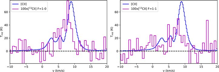
Figure 21. The [C ii] line compared with the [13C ii] F = 1–0 and F = 1–1 hyperfine transitions for the ring of RCW 36. Both [13C ii] transitions are detected and indicate that the [13C ii] emission is centered on the dip at 7 km s−1 of the [C ii] line, implying self-absorption of the [C ii] line.
Download figure:
Standard image High-resolution imageTo visualize the [O i] absorption, the spectra were integrated between 3 and 7 km s−1 (the velocities where the [O i] emission goes under the baseline in Figure 2). The resulting map is shown in Figure 22, which shows that the strongest absorption is located at the densest clumps of the ring.
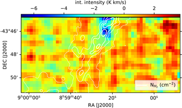
Figure 22. The [O i]-integrated intensity map from 3 to 7 km s−1, with the white contours indicating the column density. Toward the dense ring, and in particular the highest column density region, there is absorption in this velocity interval.
Download figure:
Standard image High-resolution imageAppendix C: Estimation of the FUV Field and [C ii] Temperature
In order to estimate a temperature for the gas traced by [C ii], we will work with the PDR Toolbox (Kaufman et al. 2006; Pound & Wolfire 2008), but first we must estimate the strength of the FUV field. Two methods are used to estimate the field strength independently. First, we use the method presented in Kramer et al. (2008) and Schneider et al. (2016), which makes use of the Herschel intensity at 70 and 160 μm to estimate the FUV field in Habing (Habing 1968) using

where IFIR is the far-infrared intensity from adding the intensity at 70 and 160 μm. The resulting map of the estimated FUV field strength is presented in Figure 23, which shows that the FUV field strength is generally between G0 = 300 and 2000 for RCW 36 within 1–2 pc from the cluster center. This method assumes that the [C ii] emission originates from roughly the same region as this warm dust emission, which likely is a relatively good assumption.
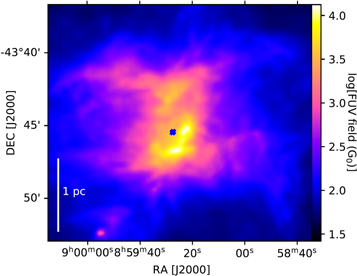
Figure 23. The FUV field map of RCW 36 on a log scale calculated from the Herschel 70 and 160 μm maps. The blue crosses indicate the locations of the O stars.
Download figure:
Standard image High-resolution imageThe second method to calculate the FUV field at a specific location, presented in Bonne et al. (2020b), directly works with the ionizing radiation intensity from the O stars in the central cluster. The FUV irradiation from these O stars is calculated from the Kurucz (1979) models with solar abundances (Grevesse & Sauval 1998). In order to select the Kurucz models to calculate the FUV field, the stellar parameters for the spectral types of the O stars were taken from Pecaut & Mamajek (2013). This results in an FUV field of G0 = 1.9 × 10³ at a distance of 1 pc and G0 = 4.7 × 10² at a distance of 2 pc. These calculations of the FUV field take no extinction on the path of the FUV photons into account, but they fit well with the values obtained from the previous method, which suggests that the FUV field at the expanding shells in the cavities is of the order of G0 = 500–2000.
From this information it is possible to estimate a temperature in the PDR using the PDR Toolbox. The surface temperature of the PDR as a function of the density is presented in Figure 24, which indicates that a surface temperature of 100–500 K is expected for an FUV field strength between G0 = 500 and 2000 and densities n = 102–105 cm−3 (Minier et al. 2013). This surface temperature of the PDR corresponds to the temperatures traced by [C ii]. To verify this method, it is also found with the PDR Toolbox that the observed [C ii] intensity of ∼100 K km s−1 toward the shells of RCW 36 fits with G0 ∼ 103 and n ∼103–104 cm−3, which is expected for the expanding shells.
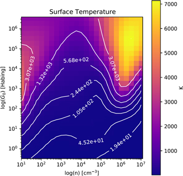
Figure 24. The surface temperature as a function of the density and FUV field in the PDR Toolbox (Kaufman et al. 2006; Pound & Wolfire 2008). Working with G0 = 500–2000 and possible densities in the shells and cavities (102 and 105 cm−3) points to temperatures between 100 and 500 K for [C ii].
Download figure:
Standard image High-resolution imageAppendix D: Fitting the X-ray Spectra
The fitting of the X-ray spectra, presented in Figure 25, uses the XSPEC package 17 (Arnaud 1996) and takes into account diffuse emission components from hot plasmas, unresolved stellar clusters, background emission, and a constant absorption from foreground material over a considered field of view. When fitting a hot plasma, the chemical abundance values from Wilms et al. (2000) are assumed. The fitting results are presented in Table 8 and Figure 25.

Figure 25. Chandra/ACIS spectra of diffuse X-ray emission in RCW 36, in the regions defined by Figure 14 and repeated in the top left panel here. This panel also demonstrates that these regions are exclusive, with no X-ray event appearing in more than one spectrum: Center and North events are color-coded in blue, Western Cavity and Southeast events are in green, and Eastern Cavity events are in red. The spectra show the total model in black, the first diffuse thermal plasma component in red, the second diffuse thermal plasma component in green, and background emission in magenta. For the Center region (top right panel), cyan curves model the emission from unresolved pre-main-sequence stars in the young cluster. Lower panels in all spectra show the fit residuals. Spectral fit parameters and model details are given in Table 8.
Download figure:
Standard image High-resolution imageTable 8. Spectral Fits for Diffuse X-Ray Regions
| Diffuse Components | ||||||||||||||||||||||
|---|---|---|---|---|---|---|---|---|---|---|---|---|---|---|---|---|---|---|---|---|---|---|
| Extraction Region | Quality | pshock1 | pshock2 | Unresolved Stars apec4+apec5 | Background apec6 | Total Diffuse Emission | ||||||||||||||||
| Name | S/N | Area | χ2/DOF | NH 1 | kT1 | τ1 | SEM1 | SB1 tc | NH 2 | kT2 | τ2 | SEM2 | SB2 tc | NH stars | SEM5 | SBstars tc | Lstars tc | NH 6 | SEM6 | SB6 tc |

|

|
| (counts) | (pc2) | (... NH: 1022cm−2 ... kT: keV ... τ: log cm−3 s ... SEM: log cm−3 pc−2 ... SB: log erg s−1 pc−2 ... L: log erg s−1 ...) | ||||||||||||||||||||
| (1) | (2) | (3) | (4) | (5) | (6) | (7) | (8) | (9) | (10) | (11) | (12) | (13) | (14) | (15) | (16) | (17) | (18) | (19) | (20) | (21) | (22) | (23) |
| Center | 1650/61 | 0.9 | 54/ 53 |

|

|

|

| 32.26 | ⋯ | ⋯ | ⋯ | ⋯ | ⋯ |

|

| 31.88 | 31.82 | 4.8* | 53.9* | 31.10 | 32.26 | 32.20 |
| Eastern Cavity | 4240/126 | 4.7 | 77/ 62 |

|

| 8.00* |

| 31.69 | 0.51* | 0.15* | 13.7* |

| 32.00 | ⋯ | ⋯ | ⋯ | ⋯ | 2.4* | 53.9* | 31.10 | 32.17 | 32.85 |
| Western Cavity | 3493/132 | 6.5 | 60/ 58 |

|

|

|

| 30.92 | 0.80* | 0.17* | 13.7* |

| 31.91 | ⋯ | ⋯ | ⋯ | ⋯ | 2.0* | 53.9* | 31.10 | 31.95 | 32.76 |
| Southeast | 5269/116 | 3.6 | 64/ 59 |

|

|

|

| 31.83 |

|

|

|

| 31.03 | ⋯ | ⋯ | ⋯ | ⋯ | 4.8* | 53.9* | 31.10 | 31.90 | 32.45 |
| North | 2207/97 | 3.1 | 39/ 40 |

|

| 13.7* |

| 31.78 | 0.36* |

|

|

| 30.81 | ⋯ | ⋯ | ⋯ | ⋯ | 4.1* | 53.9* | 31.10 | 31.83 | 32.32 |
Notes. Properties of the diffuse regions: Column (1): name of the diffuse extraction region shown in Figure 14. Column (2): signal-to-noise ratio in the total energy band (0.5–7 keV), expressed as NetCounts/σNetCounts . Column (3): geometric area of the region in square parsecs, irrespective of point-source masking, assuming a distance of 900 pc.
Details of the spectral fits: Column (4): "Reduced χ2" = χ2 divided by "degrees of freedom" for the best-fit model. All fits used the source model "tbabs1 *pshock1 + tbabs2 *pshock2 + tbabsstars (apec4 + apec5 ) + tbabs6 *apec6 " in XSPEC. NH columns report the best-fit value for the extinction column density (tbabs components). kT columns report the best-fit value for the plasma temperature (pshock and apec components). τ columns report the ionization timescale for the plasma (pshock components). SEM columns report the surface emission measure for the plasma (pshock and apec components), which is independent of distance. Unresolved pre-main-sequence stars are modeled with a pair of soft (0.86 keV) and hard (2.6 keV) thermal plasmas (apec4 + apec5 ) with a fixed normalization ratio (norm4 = 0.5 × norm5). Background emission (apec6 ) is frozen at 10 keV; its absorption (tbabs6 ) is always larger than the largest tbabs needed for other model components.
Quantities marked with an asterisk were frozen in the fit because the fit parameter ran to one of its limits or because it was poorly constrained. Uncertainties represent 90% confidence intervals. More significant digits are used for uncertainties <0.1 in order to avoid large rounding errors; for consistency, the same number of significant digits is used for both lower and upper uncertainties. Uncertainties are missing when XSPEC was unable to compute them or when their values were so large that the parameter is effectively unconstrained. SBtc and Ltc columns report the absorption-corrected surface brightness and luminosity of model components in the total band (0.5–7 keV). SB is independent of distance; L = SB × Area. SBstars and Lstars are the surface brightness and luminosity, respectively, of unresolved pre-main-sequence stars, calculated as the sum from components apec4 and apec5 . Column (22): total surface brightness from both pshock components combined. Column (23): total luminosity from both pshock components combined.
Download table as: ASCIITypeset image
The spectrum of the central region around the OB cluster is best fitted by a hot plasma and an unresolved stellar cluster. The unresolved cluster has an X-ray luminosity of 0.17 L⊙ between 0.5 and 7 keV. Converting this to a bolometric luminosity using log(Lx /Lbol) = −3.6 (Bhatt et al. 2013) gives a bolometric luminosity of 6.8 × 10² L⊙. The fitted unresolved cluster can thus correspond to low-mass stars from the 1.3 × 10⁵ L⊙ OB cluster (Verma et al. 1994) that were not resolved with ACIS. For the fitted hot plasma, the ionization timescale τ can range between 108 s cm−3 and 5 ×10¹³ s cm−3. The lower limit indicates a plasma with NEI, and the upper limit indicates a plasma with CIE. For the central region, τ thus indicates a low to intermediate timescale.
The other four regions contain no unresolved cluster and are instead fitted by two hot plasma components because a single hot plasma component did not give a satisfactory fit to the spectra. During the fit of the two plasma components in the bipolar cavities, the first plasma component went to small ionization timescales and the second one to large ionization timescales, while temperatures of both hot plasma components converged to the same temperature. Therefore, in a second run, the temperatures for both plasmas were imposed to be the same. The presence of NEI and CIE with the same temperature in the fit indicates a recombining plasma that is in transition from NEI to CIE. From the larger surface brightness in both cavities for the CIE components, it is found that the plasmas are dominated by CIE. In the region outside the H ii region, i.e., north and southeast, the temperatures of both plasma components did not converge. The first component has a temperature similar to the ones in the cavities and is likely the hot plasma that is leaking from the bipolar H ii region. The second plasma component is slightly hotter and is probably fore- or background emission, as RCW 36 is still relatively close to the Galactic plane. The surface brightness indicates that the leaking plasma is dominating the emission.
The fitting also shows that the observed diffuse X-ray emission is significantly impacted by absorption from foreground layers with NH ∼ 5 × 1021 cm−2. This is particularly seen in Column (23) of Table 8, where it is found that the intrinsic surface brightness of both cavities, corrected for absorption, is higher than for the regions outside the H ii region. Interestingly, the fitted absorbing column density value for the eastern cavity is extremely similar to the typical column density found in the Herschel maps. For the western cavity the fitting had more difficulties constraining the typical column density, so we decided to supply the foreground column density based on the Herschel data.
Appendix E: Calculating the Pressure Terms in RCW 36
The hot plasma thermal pressure is obtained from fitting the X-ray spectra, and the thermal pressure information for the ionized gas in the center is obtained from Minier et al. (2013). The thermal pressure for the ionized gas in the cavities was derived from the SHASSA Hα data (Gaustad et al. 2001). From the SHASSA data it is possible to calculate the emission measure (EM) using EM = 4.2 × 10¹⁷
Iα
after correction for the dust extinction, with Iα
the intensity in the SHASSA region. The correction for the dust extinction uses the curve from Calzetti et al. (2000) with k(λ) = 2.38, AV
= 3, based on the Herschel column density toward the cavities, and RV
= 3.1 (Draine 2003). Assuming a physical size of 1 pc for the cavities then gives an electron density of 58–62 cm−3. Combining this with an electron temperature of 8000 K then gives the thermal pressure. This method based on the SHASSA data was not applied for the central region in the ring because the associated AV
cannot be accurately constrained. To calculate the ionizing photon flux from the EM, we then use  . Here A is the surface area and αB
the recombination coefficient (=2.7 × 10⁻¹³ cm3 s−1). The radiation pressure was directly estimated using I/c, where I is the radiation intensity and c the speed of light. The radiation intensity was determined from the luminosity of the central cluster (1.3 × 10⁵
L⊙) and a distance from the cluster of 0.9 pc for the molecular ring and a distance of 1.5 pc for the cavity shells.
. Here A is the surface area and αB
the recombination coefficient (=2.7 × 10⁻¹³ cm3 s−1). The radiation pressure was directly estimated using I/c, where I is the radiation intensity and c the speed of light. The radiation intensity was determined from the luminosity of the central cluster (1.3 × 10⁵
L⊙) and a distance from the cluster of 0.9 pc for the molecular ring and a distance of 1.5 pc for the cavity shells.
To calculate the ram pressure on the expanding shells, it was assumed that they are expanding in the ambient cloud of Vela C with a density  = 102 cm–3 to 5 × 102 cm−3 and a temperature of 50 K, which is a typical temperature for the cold neutral medium. This density was estimated using a column density
  = 3 × 1021 cm−2 in the ambient cloud, based on the Herschel data, and an estimated size in the line of sight of 2–10 pc, which is poorly constrained. Inside the compressed shells of the cavities, we worked with
  = 103 cm–3 to 3 × 103 cm−3 and a temperature of 250 K that was determined from the PDR modeling. The density is estimated using a column density
  = 3 × 1021 cm−2 and a depth of 0.3–1 pc. To calculate turbulent pressure, the [C ii] line width, associated with the expanding shell (i.e., the blueshifted velocity component varying between 1 and 6 km s−1), was fitted. The details of this, for both the cavity shells and the ring, are presented in the next paragraph. To calculate the ram pressure on the molecular ring, it is assumed that the ring is expanding into an ambient cloud/sheet with
  = 103–104 cm−3 and a temperature of 20 K, which is typical for these slightly denser molecular regions in the cloud. This large range of densities was assumed, as it is difficult to constrain the density around the ridge observationally. For this estimate we assumed a typical column density around the ridge of 1022 cm−2 and a potential size range of 0.3–3 pc. To calculate the upper limit on the turbulent pressure in the ambient cloud, the velocity dispersion of 2.0 km s−1 is taken (Fissel et al. 2019). The assumed internal density of the ring is
  = 2.4 × 104 cm−3 based on a typical
  = 1.5 × 1022 cm−2 over the full ring and a diameter of 0.2 pc. The magnetic field strength in the ambient cloud was calculated using the assumed density range and the Crutcher (2012) relation. The magnetic field in the shell of the cavities was estimated using Equation (3) in van Marle et al. (2015), which assumes (initially) super-Alfvénic expansion speed, which is uncertain, leading to an upper limit. This assumption is likely not valid for the low expansion velocity of the ring, such that it is not calculated there. Future work using HAWC+ data will further address the role of the magnetic field in the ring (A. Bij et al. 2022, in preparation).
To obtain the line width of the expanding shell in the cavities, the [C ii] velocity component between 0 and 6 km s−1 was fitted with a single Gaussian. This fitting is complicated by contamination from the bright [C ii] emission at more redshifted velocities (the main velocity component associated with the ring). Therefore, a fitted Gaussian profile was only accepted if the peak brightness is between 3.5 and 40 K. This peak brightness interval covers the full observed brightness range for the velocity component below 6 km s−1, associated with the expanding shell, based on a visual inspection. As a result, this constraint prevents that the Gaussian fitting tries to include additional emission that is associated with the bright component at 7–8 km s−1 from the ring. The resulting [C ii] line width distribution for the expanding shells is presented in Figure 26.
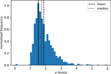
Figure 26. Histogram of the [C ii] line widths in the expanding shells in the bipolar cavities. The dashed and dotted vertical lines indicate the mean and median line width, respectively.
Download figure:
Standard image High-resolution imageFitting the line width was also done for 13CO (3–2). The resulting line width distribution for the detected emission over the full map is compared with the line width in the region that is identified as the dense ring in Figure 27. This demonstrates that there is an increase in line width toward the dense ring. To determine the associated turbulent pressure and turbulent energy in the ring, it has to be taken into account that 13CO (3–2) is optically thick there, which leads to opacity broadening given by Phillips et al. (1979),
with Δvint the intrinsic velocity dispersion we are interested in, Δv the observed velocity dispersion, and τ0 the opacity. As there is no optically thin tracer, it is not straightforward to estimate the opacity. Therefore, RADEX (van der Tak et al. 2007) was employed to estimate the optical depth. This was done using the observed line width, a typical column density  = 1.5 × 10²² for the ring, [12CO]/[H2] = 10−4, [12CO]/[13CO] = 60, Tkin 15 K, and
  = 2.4 × 104 cm−3. This gives an estimated opacity of ∼2, which results in a correction factor 1/1.35 for the line width.

Figure 27. Histogram of the 13CO (3–2) line width over the full map of RCW 36 (blue). The green histogram indicates the line width over the swept-up ring, pointing to an increased line width with respect to the rest of the mapped region of Vela C.
Download figure:
Standard image High-resolution image
Appendix F: Spitzer and Weaver Solutions
In order to estimate the expansion timescale of the different components in RCW 36, we use the Spitzer (Spitzer 1978) and Weaver (Weaver et al. 1977) solutions. First, we will discuss the Weaver solution, which is derived from Equations (51) and 52 in Weaver et al. (1977). This results in

with R the radius of the expanding structure and v the observed velocity. For the dense ring, we use R = 0.9 pc and v = 1.0–1.9 km s−1. For the shells in the cavities, we use R = 1.0 pc and v = 5.2 km s−1.
The Spitzer solution for the expansion timescale is obtained from

with ci the sound speed of the ionized gas (at a kinetic temperature Tk = 8000 K) and RSt the Strömgren radius, which is given by

with NLyC the number of photons emitted that will ionize the Strömgren radius, mp
the proton mass (=1.67 × 10⁻²⁷ kg), αB
the recombination coefficient (=2.7 × 10⁻¹³ cm3 s−1), and ρ0 the density of the neutral medium. For the number of ionizing photons we use 1048 s−1 inside the ring and 8.5 × 1046 s−1 in the cavities. This was derived based on the radio continuum for the ring and the SHASSA Hα flux for the cavities (see above). Based on the current mass in the dense ring, we can assume a density  = 2.4 × 104 cm−3 for the neutral medium, which gives texp = 1.2 Myr. However, in Section 6.5 we show that potentially half of the mass has already been removed from the central region, which would give a neutral medium density of
  cm−3 and a resulting texp = 1.7 Myr. Considering that a significant amount of mass has been removed from the region might thus increase the Spitzer expansion timescale. Even though we have argued that the hot plasma from stellar winds might drive the expansion in the cavities, we also calculated the resulting Spitzer timescale for this region. Using the above-mentioned ionizing photon flux and a neutral medium density between
  = 102 cm−3 and 5 × 102 cm−3 gives an expansion timescale between 0.2 and 0.4 Myr. These timescales are also consistent with the ones derived assuming a constant expansion velocity and confirm that, even if expansion in the cavities is driven by ionizing radiation, the expansion timescales of the cavities are short compared to the lifetime of the H ii region. All the obtained values for the expansion timescales using different methods are summarized in Table 9.
Table 9. Obtained Expansion Timescales for the Dense Molecular Ring and Cavities Assuming (1) a Constant Expansion Velocity, (2) the Weaver et al. (1977) Solution, and (3) the Spitzer (1978) Solution
| Region | Constant Velocity | Weaver et al. (1977) | Spitzer (1978) |
|---|---|---|---|
| Dense ring | 0.5–0.9 Myr | 0.3–0.6 Myr | 1.2–1.7 Myr |
| Cavities | 0.2 Myr | 0.1 Myr | 0.2–0.4 Myr |
Download table as: ASCIITypeset image
Footnotes
- 12
- 13
APEX, the Atacama Pathfinder EXperiment, is a collaboration between the Max-Planck-Institut für Radioastronomie, Onsala Space Observatory (OSO), and the European Southern Observatory (ESO).
- 14
See the equations in Section 3.2 in Beuther et al. (2002).
- 15
A factor 5 correction for the inclination assumes that we can only identify a bipolar H ii region if the inclination angle with the line of sight is larger than 70°–75°. This might be a bit of an overestimate, but most identified bipolar nebulae in Samal et al. (2018) have clearly separated cavities, which suggests that their identification is constrained to high inclination angles.
- 16
Based on the expansion timescale results, a bipolar H ii region would be identified for ∼0.2–0.5 Myr. Most mass around a H ii region might be removed in a few Myr (e.g., 1–3 Myr); see, e.g., later sections in the discussion. This suggests a correction factor of the order 5, assuming that the presence of some mass is required to identify the structure of a H ii region in the study of Spitzer images by Samal et al. (2018).
- 17