


Abstract
We report the discovery of 1RXH J082623.6−505741, a 10.4 hr orbital period compact binary. Modeling extensive optical photometry and spectroscopy reveals a ∼0.4 M⊙ K-type secondary transferring mass through a low-state accretion disk to a nonmagnetic ∼0.8 M⊙ white dwarf. The secondary is overluminous for its mass and dominates the optical spectra at all epochs and must be evolved to fill its Roche Lobe at this orbital period. The X-ray luminosity LX ∼ 1–2 × 1032 erg s−1 derived from both new XMM-Newton and archival observations, although high compared to most CVs, still only requires a modest accretion rate onto the white dwarf of  ∼ 3 × 10⁻¹¹ to 3 × 10⁻¹⁰ M⊙ yr−1, lower than expected for a cataclysmic variable with an evolved secondary. No dwarf nova outbursts have yet been observed from the system, consistent with the low derived mass-transfer rate. Several other cataclysmic variables with similar orbital periods also show unexpectedly low mass-transfer rates, even though selection effects disfavor the discovery of binaries with these properties. This suggests the abundance and evolutionary state of long-period, low mass-transfer rate cataclysmic variables are worthy of additional attention.
Export citation and abstract BibTeX RIS
1. Introduction
1.1. Observational Appearance of Cataclysmic Variables
Binary stars containing a white dwarf accreting from a dwarf of a subgiant companion are called cataclysmic variables (Warner 1995; Hellier 2001). They earned this name thanks to two types of violent phenomena that may dramatically increase the optical brightness of such binaries: classical nova eruptions and dwarf nova outbursts. A classical nova eruption occurs when thermonuclear reactions ignite in the accreted hydrogen-rich shell (Bode & Evans 2008; Starrfield et al. 2016; Chomiuk et al. 2021), typically leading to a high (∼8–15 mag; Vogt 1990; Warner 2008; Kawash et al. 2021) outburst amplitude. A dwarf nova outburst is powered by a completely different physical mechanism. These more modest outbursts (typically ∼2–8 mag; Coppejans et al. 2016; Kawash et al. 2021) occur when the accretion disk surrounding a white dwarf switches from a low-viscosity, low-accretion-rate state with an emission-line-dominated spectrum 14 to a high-viscosity, high-accretion-rate continuum-dominated state. This disk instability model for the dwarf nova phenomenon has been extensively discussed in the literature (Osaki 1996, 2005; Hameury 2020; Done et al. 2007). Dwarf novae occur if the mass-transfer rate is insufficient to maintain the accretion disk permanently in the hot high-viscosity state and if the accretion disk formation is not disrupted by the strong magnetic field of the white dwarf (Cropper 1990; Patterson 1994; Ferrario et al. 2015).
Cataclysmic variables are often prominent X-ray sources (Mukai 2017). While in classical novae X-rays are emitted by plasma heated by nuclear burning and shocks within the nova ejecta, X-rays from non-nova cataclysmic variables are powered by accretion. Specifically, the X-rays emerge at the interface between the accretion disk/stream and the white dwarf surface, known as the boundary layer. The exact structure of this region, the role of shocks and magnetic field, as well as changes accompanying the disk state transitions are debated (e.g., Popham & Narayan 1995; Pandel et al. 2005; Ishida 2010; Datta et al. 2021). The optically thin thermal X-ray emission of cataclysmic variables has the maximum temperature  = 6–55 keV and luminosity 1028–1032 erg s−1 (Balman 2020). If the accretion disk is disrupted by the white dwarf's magnetosphere, the matter reaches the white dwarf surface via the accretion columns above the magnetic poles (Wu 2000; Mouchet et al. 2012). The X-ray emission of magnetic cataclysmic variables is characterized by a maximum temperature of a few tens of keV and spans the range of luminosities from 1030 to 1034 erg s−1 (de Martino et al. 2020). The white dwarf rotation moves the accretion columns in and out of view, modulating the X-ray flux. These periodic variations, together with the generally harder X-ray spectra, are the telltale signs of magnetic cataclysmic variables.
1.2. Origin and Evolution of Cataclysmic Variables
Cataclysmic variables are thought to have evolved from binaries that survived a common-envelope phase without merging (Paczynski 1976; Ritter 2010; Ivanova et al. 2013). The typical stages are as follows. As the more massive star in a wide separation binary evolves into a red giant, it may overflow its Roche lobe, starting mass transfer to its less massive companion. As the convective envelope of the red giant expands due to mass loss on a dynamical timescale and the binary orbit shrinks due to the conservation of angular momentum, this is a runaway process (Paczyński and Sienkiewicz 1972), causing the components to be engulfed in a common envelope on a dynamical timescale. The successful ejection of the envelope will lead to a hardened binary containing a white dwarf and the original secondary.
While mass transfer from a more massive to less massive binary component is unstable, the opposite process is sustainable, and in principle, mass transfer can begin from the secondary to the white dwarf if the secondary fills its Roche Lobe during the main sequence or later evolution. This is the stage where the binary would become observable as a cataclysmic variable. Transferring mass from a less massive to a more massive component brings the accreted matter closer to the binary center of mass, requiring the component separation to increase in order to conserve angular momentum, which tends to break contact between the binary components. An additional physical mechanism, either angular momentum loss or an expansion of the secondary in response to mass loss, is needed to restore and maintain contact.
1.2.1. The Canonical Evolution Path
The common wisdom is that cataclysmic variable evolution is driven by secular angular momentum loss that keeps the binary components in contact (e.g., Knigge et al. 2011). The two relevant physical mechanisms are gravitational-wave emission (Paczyński 1967; Paczynski & Sienkiewicz 1981), dominating in systems with orbital periods less than 3 hr; and magnetic braking (Mestel 1968; Verbunt & Zwaan 1981), dominating at longer periods. Magnetic braking occurs due to magnetic coupling between the star and its ionized stellar wind carrying away angular momentum. As the secondary star in a cataclysmic variable is tidally locked (its axial rotation period is equal to the orbital period), the angular momentum loss due to the magnetized wind has to be compensated by decreasing orbital period. Once the secondary star loses enough mass to become fully convective (corresponding to the orbital period of about 3 hr), the effectiveness of the magnetic braking appears to be dramatically reduced (Spruit & Ritter 1983; Verbunt 1984). Most interacting systems lose contact when evolving to periods shorter than 3 hr and remain detached until gravitational-wave emission brings the components back in contact at periods of about 2 hr, leading to an observed gap in cataclysmic variable periods between ∼2 and 3 hr (Kolb et al. 1998; Howell et al. 2001).
It is possible that other angular momentum loss mechanisms operate in cataclysmic variables in addition to gravitational radiation and magnetic braking. Angular momentum loss may happen during nova eruptions (Schenker et al. 1998; Schreiber et al. 2016; Pala et al. 2022). Indeed, each nova eruption is akin to a common-envelope phase (Nelemans et al. 2016; Sparks & Sion 2021), with the white dwarf atmosphere expanding to engulf both binary components. Other possibilities discussed in the literature include angular momentum losses via a circumbinary disk (Willems et al. 2005) and magnetized accretion disk wind (Cannizzo & Pudritz 1988). Nova eruptions may also heat (and inflate) the secondary, increasing the mass-transfer rate above its mean long-term value (Ginzburg & Quataert 2021).
Cataclysmic variables evolve toward short periods until the thermal timescale of the secondary becomes longer than the mass-transfer timescale, which leads to an increase rather than a decrease in the orbital period in response to mass loss. The minimum period is about 80 minutes (e.g., Tutukov et al. 1985; Gänsicke et al. 2009) for ordinary hydrogen-rich donors and is shorter for helium-rich donors (that have smaller sizes for a given mass).
1.2.2. The Alternative: Nuclear Evolution of the Donor
Contact between the binary components can be maintained without major angular momentum loss if the donor is expanding due to nuclear evolution. A well-understood case is if the donor is less massive than the white dwarf and can transfer mass as a subgiant or red giant, with the orbital period and mass-transfer rate growing with time (Webbink et al. 1983; Pylyser & Savonije 1988; Goliasch & Nelson 2015). Another possibility arises if the donor star is more massive than the white dwarf after the common-envelope phase. In this case, there can be an initial phase of thermal timescale mass transfer once the donor fills its Roche Lobe as a subgiant. This reduces the orbital period until the two components have similar masses. After that, mass transfer proceeds on a timescale governed by magnetic braking and/or nuclear evolution (e.g., Ivanova & Taam 2004; Kalomeni et al. 2016).
1.3. 1RXH J082623.6−505741 and the Scope of this Work
1RXH J082623.6−505741 originally drew our attention as a possible X-ray counterpart of the Fermi-LAT γ-ray source 3FGL J0826.3−5056. Once our initial optical spectroscopy showed it to be a Galactic source with evidence for ongoing accretion, we started a multiwavelength campaign. With the subsequent release of the Fermi-LAT Pass 8 data (Bruel et al. 2018), and eventually the 4FGL (and 4FGL Data Release 2) catalogs (Abdollahi et al. 2020; Ballet et al. 2020), the location of the γ-ray source "moved" to the northeast, leaving 1RXH J082623.6−505741 well outside the 95% error ellipse of the revised γ-ray position (now dubbed 4FGL J0826.1−5053). The optical Gaia EDR3 (Gaia Collaboration et al. 2021) counterpart of 1RXH J082623.6−505741 has an ICRS position of 08:26:23.801, −50:57:43.46 at the mean epoch 2016.0 and a highly significant parallax measurement (ϖ = 0.583 ± 0.036 mas), resulting in a distance of 1.63 ± 0.09 kpc after applying a zero-point offset of −0.0294 mas (Lindegren et al. 2021); because of the precise measurement, the prior on the distance is not important. The mean optical magnitude of 1RXH J082623.6−505741 is V = 16.60 ± 0.06 (Henden et al. 2015), corresponding to an absolute magnitude of MV ∼ 5.0–5.2, depending on the extinction adopted (see discussion in Section 3.3).
Here we report on optical, X-ray, and radio observations of 1RXH J082623.6−505741 that, although unrelated to 4FGL J0826.1−5053, was revealed to be a cataclysmic variable star with an evolved secondary. We derive the parameters of the binary system and discuss them in the context of the cataclysmic variable population and evolution. The inferred low mass-transfer rate of this binary is challenging to explain with the current cataclysmic variable evolution theory.
2. Observations
2.1. X-Ray
2.1.1. XMM-Newton
We performed a dedicated XMM-Newton observation of 1RXH J082623.6−505741 (as a candidate GeV source counterpart; Section 1) for 48 ks starting on 2017 June 13 21:44:37 TDB (ObsID 0795710101). The observation start time corresponds to the orbital phase of 0.76 and covers almost 1.3 orbital periods of the system (Section 3.1). The Medium filter was used for the three European Photon Imaging Camera (EPIC) instruments. The source is clearly visible with 1437 (0.021 ± 0.001 cts s−1), 1527 (0.025 ± 0.001 cts s−1), and 3404 (0.083 ± 0.003 cts s−1) photons attributable to the source detected by the first and second EPIC-Metal Oxide Semiconductor (MOS1 and MOS2; Turner et al. 2001) and EPIC-pn (Strüder et al. 2001) cameras, respectively, in the 0.2–10 keV energy range. The source is too faint for grating spectroscopy with the Reflection Grating Spectrometers (den Herder et al. 2001).
We used xmmsas_20190531_1155-18.0.0 (Gabriel et al. 2004) for reducing the EPIC data. After the initial data ingestion cifbuild, odfingest, and pipeline-processing emproc/epproc steps, we constructed pattern zero (single-pixel events) only, high-energy lightcurves used to identify times of high particle background. To construct these lightcurves, we apply filtering on the Pulse Invariant channel number (PI; encoding the photon energy) and pixel pattern triggered by a photon or a background charged particle (PATTERN; sometimes referred to as "event grade"). We apply the following evselect filtering expressions: (PI>10000) && (PATTERN==0) for MOS1/2 and (PI>10000 && PI<12000) && (PATTERN==0) for pn cameras, respectively. After a visual inspection, we selected low background good time intervals with RATE<=0.2, <=0.25, <=0.4 for the three cameras, respectively. Comparing these thresholds to reference values in the EPIC analysis thread, 15 the MOS1/2 cutoff levels are relatively aggressive, while the pn cutoff matches the reference value. These cutoffs result in about 5% of MOS1/2 and almost 50% of pn data being rejected.
We converted the photon arrival times to the solar system barycenter with barycen. After producing the images with evselect, we used ds9 to center a 20'' radius circular aperture on the source image (independently for the three instruments). For background extraction, we used a source-centered annulus with the inner and outer radii of 39'' and 91'' (140'' and 162 5) for MOS1 (MOS2) and an off-source circle 94'' radius circle for pn. These regions were chosen to avoid nearby sources and check that the analysis results do not depend strongly on the specific choice of the background region. We extracted source and background spectra from the respective regions with evselect applying filtering: (PI>150) for all three cameras; (PATTERN<=12) for MOS1/2 and (PATTERN<=4) for pn cameras, respectively. The associated calibration parameters were generated with backscale, rmfgen, and arfgen. We used specgroup to bin the spectra to contain at least 25 background-subtracted counts per bin and not to oversample the intrinsic energy resolution by a factor > 3. We also extracted event files (unbinned lightcurves) for the source and background regions. Finally, we used evselect ((PATTERN<=4) && (PI in [200:10000])) and epiclccorr to construct background-subtracted 0.2–10 keV lightcurves with 300 s time binning (so, on average, the lightcurves contain 6.3, 7.5 and 24.9 counts per bin for MOS1/2, pn).
Figure 1 presents the binned lightcurve (48 ks) of 1RXH J082623.6−505741. No systematic change in brightness is seen during the observation; however, the χ2 test indicates that the lightcurve scatter is significantly larger than expected from the error bars (de Diego 2010; Sokolovsky et al. 2017). This suggests the presence of irregular variations on timescales comparable to or longer than the 300 s bin size and shorter than the 48 ks duration of the lightcurve.

Figure 1. XMM-Newton/EPIC 0.2–10 keV background-subtracted lightcurve of 1RXH J082623.6−505741. A minimal amount of the MOS 1/2 data was rejected due to background contamination, but the figure is much larger for the pn data, nearly 50%. Nonetheless, the vast majority of the potential 300 s bins for the pn lightcurve are usable, as they had at least a partial uncontaminated time interval. There is no systematic change in the count rate during the observation.
Download figure:
Standard image High-resolution imageThe discrete Fourier transforms of the lightcurves (Deeming 1975; VanderPlas 2018) show no obvious periodicities in the range of 600 s (2× time bin width) to 5000 s (1/10 of the observation duration). The need to obtain a significant estimate of the count rate within a bin limits our ability to search for periods about or shorter than the bin width. This can be avoided by performing the period search on the photon arrival times recorded in the event file directly, with no binning (e.g., Jackman et al. 2018).
Background subtraction is not possible for the unbinned lightcurve as it is not clear if a given event recorded within the source aperture should be attributed to the source or background. This is not a show stopper as the constant background should just reduce the pulsed fraction and add noise to the periodic signal. The background flares (produced by an increased number of charged particles hitting the detector) are not periodic but may introduce "red noise" in the power spectrum with some of its power leaking to high frequencies where we conduct the period search (see the discussion in Appendix). While the time intervals obviously affected by an increased particle background are rejected from the analysis, some residual particle background variations remain. Period searches on the events extracted from the background region are used to identify any spurious periodicities introduced by residual background variations and the efforts to reject visible background flares, as well as check for the presence of any periodic instrumental effects.
We performed a discrete Fourier transform (Rayleigh test) and an "Hm
periodogram" search in the trial period range from 0.5 s (3.0 s for MOS1/2 as "Full Frame" mode frame time is 2.7 s) to 5000 s as described in Appendix. No periodogram peak was identified that was both significant according to the Hm
statistic (de Jager et al. 1989; de Jager & Büsching 2010; Kerr 2011) and appeared at similar frequencies in lightcurves collected with multiple instruments. We confirmed this conclusion by repeating the analysis with another code, implementing the closely related " periodogram" (Buccheri et al. 1983, see the discussion in Appendix) applied to the pn data in the 0.3–8 keV, 0.3–2 keV, and 2–8 keV energy ranges.
Previously, five XMM-Newton slews (Saxton et al. 2008) over the 1RXH J082623.6−505741 area in 2005–2013 led to 2σ 0.2–12 keV EPIC-pn upper limits of ≲1 cts/s, according to the Upper Limit Server 16 (Saxton & Gimeno 2011). Therefore, the source could not have been much brighter during these slews compared to the long XMM-Newton observation.
The spectra obtained with the three EPIC cameras during the dedicated observation on 2017 June 13 are grouped with specgroup to contain at least 25 counts per energy bin. We adopt χ2 as the fit and test statistic and fix the elemental abundances to the solar values as derived by Asplund et al. (2009). We simultaneously fit the spectra obtained by the three EPIC cameras with an absorbed single-temperature optically thin thermal emission model (Figure 2). Specifically, we use the XSPEC model const∗phabs∗cflux(apec), where const is an offset between the cameras, phabs is the photoelectric absorption model (Balucinska-Church & McCammon 1992), cflux is the convolution model needed only to calculate the flux of the next model component, and apec is the collisional ionization equilibrium plasma emission model that includes both bremsstrahlung continuum and line emission (Brickhouse et al. 2005). The fit results in χ2/Nd.o.f. = 122.4/133). The best-fit model parameters and their associated 1σ uncertainties are the equivalent hydrogen-absorbing column density  cm−2, plasma temperature
  keV, and unabsorbed flux
  erg cm−2 s−1 at 0.2–10 keV. The scaling factor was fixed to 1.0 for the pn camera and the best-fit values were 0.95 and 1.04 for MOS1 and MOS2. The Fe Kα emission at 6.7 keV is clearly visible in the pn spectrum (Figure 2) and is well described by the apec model with Asplund et al. (2009) abundances.
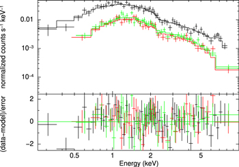
Figure 2. XMM-Newton spectra of 1RXH J082623.6−505741 obtained with the three EPIC cameras (pn—black, MOS1—red, MOS2—green) compared to the absorbed optically thin thermal emission model.
Download figure:
Standard image High-resolution imageThe fitted NH is consistent within 1σ with the integrated Galactic NHI value derived from 21 cm hydrogen line observations (Kalberla et al. 2005; Bajaja et al. 2005; Kalberla & Haud 2015). However, much of this absorbing material likely lies beyond the binary. Instead, using the E(B − V) value favored from the spectroscopy (Section 3.3) and the relation of Güver & Özel (2009) between the X-ray absorbing column and optical extinction (NH = 2.21 × 1021 cm−2 AV ), we infer a foreground NH ∼ 7 × 10²⁰–1.2 × 1021 cm−2, depending on which interstellar Na i absorption to dust extinction relation we adopt (see Section 3.3). Güver & Özel 2009 report a 4% uncertainty in the slope of the NH(AV ) relation. It is unclear what the intrinsic scatter of this relation is as the individual pairs of NH and AV measurements used by Güver & Özel (2009) have large uncertainties. 1RXH J082623.6−505741 is located in a scenic region of the sky next to a dark nebula and multiple Herbig–Haro objects including HH 46/47 (6' away in the foreground at 450 pc Noriega-Crespo et al. 2004). The extinction law and dust-to-gas ratio variations found in the vicinity of star-forming regions (Gómez de Castro et al. 2015; Liseau et al. 2015; Tricco et al. 2017, e.g.) further complicate the optical extinction. While the overall uncertainty of the AV -based estimate of NH is difficult to quantify, it is unclear if it can account for almost a factor of 3 difference with the X-ray-derived NH. Therefore, a fraction of the measured NH may be intrinsic to 1RXH J082623.6−505741.
At the Gaia parallax distance to the source, the inferred unabsorbed X-ray flux corresponds to a 0.2–10 keV luminosity of LX = (1.6 ± 0.1) × 1032 erg s−1, which we use for the remainder of the paper.
As the X-ray spectra of many cataclysmic variables are described in terms of the multitemperature cooling flow model (e.g., Balman 2020), we fit the model constant∗phabs∗mkcflow (Mushotzky & Szymkowiak 1988) to the EPIC data. The highest temperature of the cooling flow is k
T = 43 ± 10 keV and the absorbing hydrogen column  cm−2 (close to the one inferred from the single-temperature model). The accretion rate derived from mkcflow is 3 × 10⁻¹¹
M⊙ yr−1, about the same as what we derive from the apec fit. The fit is acceptable with χ2/Nd.o.f. = 86.46/107; however, it does not improve on the simpler single-temperature plasma model that we use throughout this paper.
cm−2 (close to the one inferred from the single-temperature model). The accretion rate derived from mkcflow is 3 × 10⁻¹¹
M⊙ yr−1, about the same as what we derive from the apec fit. The fit is acceptable with χ2/Nd.o.f. = 86.46/107; however, it does not improve on the simpler single-temperature plasma model that we use throughout this paper.
2.1.2. Swift
The Neil Gehrels Swift Observatory (Gehrels et al. 2004) observed 1RXH J082623.6−505741 in the Photon Counting mode for a total of 7.5 ks between 2015 March 25 and 2017 March 3 (Table 1). The observations were obtained in the framework of a program to follow up Fermi unassociated sources 17 (Stroh & Falcone 2013). 1RXH J082623.6−505741 is clearly visible in the stacked Swift X-ray Telescope (XRT; Burrows et al. 2005) 0.3–10 keV image with the net count rate of 0.0071 ± 0.0012 cts s−1. We used WebPIMMS 18 to predict the XMM-Newton/EPIC-pn + Medium filter + Full Frame mode count rate of 0.081 assuming the thermal plasma model from Section 2.1.1. This closely matches what was actually observed by XMM-Newton/EPIC-pn (Section 2.1.1), suggesting a similar X-ray flux in the Swift/XRT data compared to the XMM-Newton data. We group the stacked Swift/XRT spectrum with grppha to contain at least nine counts per bin and fit with the model used in Section 2.1.1 for the XMM-Newton observations fixing the kT and NH values and leaving only the model normalization factor free to vary (χ2/Nd.o.f. = 1.86/4; Figure 3), indicating no compelling evidence for a different spectrum in the Swift/XRT data compared to the higher signal-to-noise XMM data.
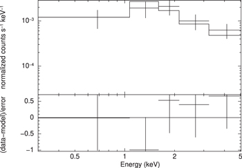
Figure 3. The stacked Swift/XRT spectrum of 1RXH J082623.6−505741 compared to the absorbed optically thin thermal emission model.
Download figure:
Standard image High-resolution imageTable 1. Swift Observing Log
| Obs.ID | Date | Exposure (s) |
|---|---|---|
| 00084684001 | 2015-03-25 | 763 |
| 00084684002 | 2015-06-01 | 393 |
| 00084684003 | 2015-08-30 | 183 |
| 00084684004 | 2015-09-23 | 597 |
| 00084684005 | 2015-10-01 | 1660 |
| 00084684006 | 2017-03-03 | 3939 |
Download table as: ASCIITypeset image
2.1.3. ROSAT
The Upper Limit Server lists a pointed 20 ks ROSAT/HRI observation of the 1RXH J082623.6−505741 area on 1994 May 12. The source is detected with the 0.2–2 keV HRI count rate of 0.0012 ± 0.0004 cts s−1. The source is listed as 1RXH J082623.6−505741 by the ROSAT Scientific Team (2000). The upper limits server lists no pointed ROSAT/PSPC data; however, the source was observed in the survey mode (Voges et al. 1999, 2000; Boller et al. 2016) on 1990 October 30, resulting in a 2σ 0.2–2 keV PSPC upper limit of <0.022 cts/s. Using WebPIMMS to extrapolate the ROSAT/HRI detection to the XMM-Newton/EPIC-pn band using the absorbed thermal plasma model derived from the XMM-Newton observations described in Section 2.1.1, we estimate an XMM-Newton/EPIC-pn + Medium filter + Full Frame mode count rate of 0.038 cts s−1, a factor of 2 lower than what was actually observed. This may suggest a factor of ∼2 X-ray flux variability on a decades-long timescale.
2.2. Optical Spectroscopy
2.2.1. SOAR
Using the Goodman Spectrograph (Clemens et al. 2004) mounted on the 4.1 m SOAR telescope, we obtained optical spectroscopy of 1RXH J082623.6−505741 on parts of 13 nights from 2016 December 30 to 2019 November 6. The main setup used a 1200 lines mm−1 grating with a 095 slit, giving an FWHM resolution of about 1.9 Å over the wavelength range 5500–6750 Å. Depending on the seeing, the exposure time per spectrum was 900 or 1200 s. Spectral reduction and optimal extraction were performed in the usual manner using IRAF (Tody 1986). A SOAR/Goodman spectrum covering a wider wavelength range of 3600–6850 Å (400 lines mm−1 grating, 1'' slit) obtained on 2016 December 30 is presented in Figure 4.
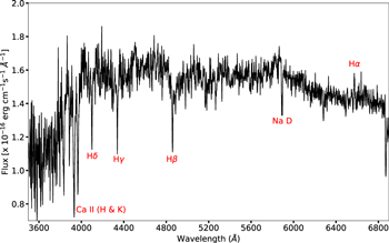
Figure 4. Low-resolution SOAR/Goodman spectrum of 1RXH J082623.6−505741 from 2016 December 30. At this epoch, the emission from the accretion disk was relatively faint compared to the cool secondary star, which dominates the optical emission. An approximate flux calibration has been applied to the data.
Download figure:
Standard image High-resolution image2.2.2. Magellan
To assess the rotational broadening of the secondary, we obtained on 2019 April 6 a single 2400 s high-resolution spectrum of the system with MIKE (Bernstein et al. 2003) on the Magellan/Clay Telescope. Data were accumulated on both the blue and red sides of the instrument, with resolutions of R ∼ 30,000 and ∼26,000, respectively. The data were reduced using CarPy (Kelson 2003).
2.3. Optical Photometry
We obtained 226 B-, 228 V-, and 226 I-band photometric measurements using ANDICAM on the SMARTS 1.3 m telescope at CTIO over 228 nights between 2017-01-08 and 2018-04-29. The data reduction is described by Walter et al. (2012). The estimated photometric uncertainties are 0.050, 0.026, and 0.022 mag in the B, V, and I bands, respectively. The lightcurve (Figure 5) shows a 0.06 mag increase in mean brightness over the duration of the observations as well as a short-term modulation, but no flaring activity.
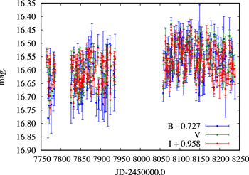
Figure 5. SMARTS 1.3 m ANDICAM BVI lightcurve of 1RXH J082623.6−505741.
Download figure:
Standard image High-resolution imageAfter detrending the lightcurve with a piecewise linear function, applying the barycentric correction (e.g., Eastman et al. 2010), and combining B, V, and I lightcurves removing the median offsets of (B − V) = 0.727 and (V − I) = 0.958, we performed a period search using the string-length technique of Lafler & Kinman (1965), resulting in the following light elements:

We identify the light-variation period with the orbital period of the binary system, the conclusion confirmed with spectroscopy discussed in Section 3.1. The period uncertainty is calculated allowing for the maximum phase shift of 0.05 between the first and the last observation; see Appendix. The phased lightcurve is presented in Figure 6. The epoch of the primary minimum in Equation (1) corresponds to the orbit phase of 0.75 defined in Section 3.1.
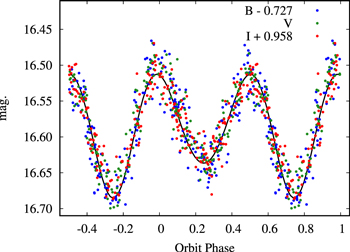
Figure 6. SMARTS 1.3 m ANDICAM BVI lightcurve of 1RXH J082623.6−505741 phased with the photometric period (Equation (1)) and the spectroscopically derived minimum radial velocity phase T0BJD(TDB) (Section 3.1) for consistency with Figure 8. The curve represents the model described in Section 3.4.
Download figure:
Standard image High-resolution imageWe choose the Lafler & Kinman (1965) period search technique as it is suitable for phased lightcurves of an arbitrary form (they do not have to be sine-wave like) and the lightcurve at Figure 6 has unequal minima. While the visual inspection of the phased lightcurve leaves no doubt that the brightness variations are real, we confirm this by performing formal tests. We use bootstrapping (e.g., Section 7.4.2.3. of VanderPlas 2018) to test the chance occurrence probability of the periodicity detected with the Lafler & Kinman (1965) technique. We also construct the Lomb–Scargle periodogram (Lomb 1976; Scargle 1982; VanderPlas 2018) and use Equation (14) of Scargle (1982) to estimate the significance of its highest peak (corresponding to half the orbital period). We follow Appendix to estimate the number of independent frequencies needed for the Lomb–Scargle peak significance calculation. Both bootstrapping and analytical calculation point to the chance occurrence probability of the periodic signal to be ≪ 10−4.
Nothing is visible in the GALEX near-UV (2310 Å) image covering the source position (Bianchi et al. 2017). The XMM Optical Monitor observations that accompanied our X-ray data were taken in V rather than in the UV and hence offer no additional UV constraints.
2.4. Radio
We obtained radio continuum observations of 1RXH J082623.6−505741 with the Australia Telescope Compact Array on 2017 March 3, while the array was in its 6D configuration (5.9 km maximum antenna spacing) and using the 5.5/9.0 GHz backend (we only consider the lower-noise 5.5 GHz observations here). The on-source integration time was 10.2 hr, and we used PKS 0823−500 as the complex gain calibrator and PKS 1934−638 as the flux density and bandpass calibrator. The data were reduced and imaged using standard tasks in CASA (McMullin et al. 2007), with the imaging done with a Briggs robust value of 1. The rms noise in the final 5.5 GHz image was 7 μJy bm−1, and a radio continuum counterpart for 1RXH J082623.6−505741 was not detected, with a 3σ upper limit of <21 μJy.
3. Results & Analysis
3.1. Optical Spectra and Radial Velocities
The SOAR spectra show the same qualitative features: A range of stellar photospheric absorption lines along with resolved, broad Hα and double-peaked He I lines in emission that vary in prominence among the spectra (Figure 7). We derived radial velocities of the secondary through a cross-correlation of the wavelength range 6050–6250 Å, which is dominated by absorption lines. For the cross-correlation, we used an early-K-star template, which on average provided higher cross-correlation peaks than mid-G or late-K templates. There was no evidence for more than one set of absorption lines in any of the SOAR or MIKE spectra. The emission lines associated with the accretion disk (and possibly partly with the other structures in the system, such as the hot spot) form a second set of lines. While the double-peaked emission lines indicate origin in an accretion disk around the white dwarf, it requires data with high signal-to-noise ratio in the line wings to make reliable radial velocity measurements of the white dwarf, free of interferences from other components such as the bright spot. Because this is not the case here, we effectively have a single-lined spectroscopic binary.
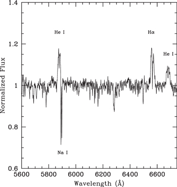
Figure 7. Continuum-normalized moderate-resolution SOAR/Goodman spectrum taken on 2017-11-15. Double-peaked emission lines of He i at 5875 and 6678 Å and H i at 6563 Å from the accretion disk are evident, as are the numerous narrow metal absorption lines from the secondary. The resonance Na i line is a blend of absorption from the secondary and the interstellar medium.
Download figure:
Standard image High-resolution imageWe first fit a circular model to the radial velocities using the custom Monte Carlo sampler TheJoker (Price-Whelan et al. 2017). Each of the posterior distributions is close to normal, and the samples are essentially uncorrelated except for a weak correlation between the period P and epoch of the ascending node of the white dwarf T0. The best-fitting parameters are P = 0.4316979(17) days, T0BJD(TDB) = 2457758.78073 ± 0.00102 days, semiamplitude K2 = 175.3 ± 2.4 km s−1, and systemic velocity γ = 35.0 ± 1.8 km s−1. This best-fitting circular model had χ2/Nd.o.f. = 35.7/30 with an rms of 9.7 km s−1 and is shown in Figure 8. This orbital period value matches that found from the optical photometry (Section 2.3) within the relative precision of the two measurements.

Figure 8. Radial velocity measurements of the secondary star, phased on the best-fit circular Keplerian model.
Download figure:
Standard image High-resolution imageAn eccentric fit with six free parameters had a posterior eccentricity (e) distribution peaked at 0, with a median e = 0.014 ± 0.013 and a slightly worse χ2/Nd.o.f. = 33.7/28 than the circular fit. Hence, there is no compelling evidence for a deviation from the simple circular model.
Fitting only the spectra obtained at orbital phases ϕ = 0.125–0.375 (the side of the secondary without direct heating) gives K2 = 183 ± 8 km s−1, identical within the uncertainties to the value for the full fit. We find no evidence that heating is meaningfully affecting our original K2 measurement, which we use for the remainder of the paper.
For the subset of spectra with well-defined Hα emission profiles, we find a mean FWHM of 1400 ± 80 km s−1 and a mean peak separation of the blue and red Hα peaks of 760 ± 60 km s−1. These values are within the range of those observed for accreting white dwarfs (e.g., Casares 2015, 2016). The mean equivalent width of Hα, ∼4–5 Å, is relatively low for an accreting white dwarf but consistent with an evolved, relatively luminous secondary (see Section 4.4).
3.2. Rotational Velocity
While our typical SOAR spectra have a modest FWHM resolution of about 85 km s−1, in some spectra there is nevertheless evidence for line broadening, as would be present if the projected rotational velocity ( ) of the secondary was being observed. Given that the synchronization timescale for 1RXH J082623.6−505741 is ≲103 yr at the orbital period and mass ratio derived above, we expect the visible secondary to be tidally locked.
To test if the absorption lines associated with the donor star are indeed broadened, we first analyze the single high-resolution MIKE spectrum of the binary (Section 2.2.2). Following Swihart et al. (2017), we take a set of spectra of stars with similar spectral type and negligible rotation obtained with the same instrument setup. In order to simulate the rotational broadening of spectral lines, we convolve these template spectra with convolution kernels corresponding to a range of rotational velocities and assuming a standard limb-darkening law. We then cross-correlate these convolved templates with the set of original unbroadened spectra to obtain a set of relationships (N2 for N templates) between the observed line broadening and  . In effect, we construct the relationship of line FWHM versus
  from the templates and then use it to derive
  from the observed FWHM. One change we make, specific to this source, is to account for the motion of the secondary over the length of the exposure; while we deliberately obtained the spectrum relatively close to conjunction, the range of phases (ϕ = 0.407 to 0.471) still corresponds to a motion of about 26 km s−1 using the best-fit orbital model described in Section 3.1. We simulate this by shifting the standard star spectra by small amounts appropriate to the varying velocity over the exposure and then averaging over these spectra. As it turns out, this motion is much smaller than the measured value of
  , and so this effect was essentially negligible. The inferred mean intrinsic FWHM for the MIKE spectra is 133 ± 12 km s−1.
Using a range of orders with good signal-to-noise ratio in the absorption features, but avoiding emission lines, telluric features, and spectral regions with substantial sky features, we found  km s−1. The uncertainty is dominated by the spread in values between different spectral orders rather than the spread among templates, which is much smaller. The precision of the measurement is somewhat lower than typical, which could be due to the modest signal-to-noise ratio of the spectrum or to the presence of the accretion disk.
As a check on the result from this single MIKE spectrum, we repeated this  analysis using the moderate-resolution (1200 l mm−1) SOAR spectra, finding a value of 83 ± 3 km s−1. The uncertainty is the error of the mean derived from 24 spectra with a high-enough signal-to-noise ratio for this analysis (the measured standard deviation is 14 km s−1). That these values agree is reassuring, though it does not fully capture all systematic uncertainties in this analysis, such as the choice of limb-darkening law.
Given the short period and accreting nature of the system, it is reasonable to assume the nondegenerate secondary is indeed tidally synchronized so that its rotational period matches the orbital period. In this case, we can use the Eggleton (1983) Roche Lobe approximation, which relates  and the measured radial velocity semiamplitude K2 to the mass ratio:

where q = M2/M1 is the mass ratio. Indeed, the observed axial rotation velocity of the secondary

where R2 is the secondary star radius. The observed maximum orbital velocity of the secondary

where a/(1 + q) is the distance between the secondary star and the system's center of mass, while a is the binary separation. We obtain Equation (2) by dividing Equation (3) by Equation (4) and using the Eggleton (1983) approximation for R2/a. The optically derived mass ratios using Equation (2), e.g., the ones obtained by Strader et al. (2015) and Swihart et al. (2019), have been shown to be reliable for many compact binaries when compared with the direct mass-ratio measurements from pulsar timing (Strader et al. 2019). The values of  and K2 given above imply q = 0.49 ± 0.09 for 1RXH J082623.6−505741.
3.3. Extinction
While the integrated line-of-sight reddening in this direction is high (E(B − V) = 0.82; Schlafly & Finkbeiner 2011), all the observational data are consistent with a lower extinction, likely due to the relatively nearby distance of the binary. We estimate the extinction from the high-resolution MIKE spectrum, which allows a clean separation of intrinsic absorption lines from the interstellar ones. Using the Na i calibration of Poznanski et al. (2012), we found E(B − V) = 0.10 ± 0.04. The calibration of Munari & Zwitter (1997), which only uses the bluer stronger component of Na i, gives a somewhat higher value of E(B − V) = 0.18 ± 0.05. The results from lightcurve fitting favor a value at the lower end of this range, with E(B − V) ≲ 0.1 (Section 3.4).
3.4. Light-curve Modeling
The unabsorbed 0.2–10 keV X-ray luminosity of 1.6 × 1032 erg s−1 in our XMM-Newton data, combined with previous Swift and ROSAT detections, shows a consistently high LX that implies 1RXH J082623.6−505741 is a compact binary. Further evidence is provided by luminous double-peaked He i and H i lines from optical spectra that are consistent with the presence of an accretion disk.
Given the optical lightcurves show clear evidence for ellipsoidal variations (Figure 5), we undertook lightcurve modeling of the SMARTS BVI data to constrain the binary inclination. We used the Eclipsing Light Curve (ELC; Orosz & Hauschildt 2000) code, which models filter-specific lightcurves in each band independently. In all our models, we assumed a compact, invisible primary surrounded by an accretion disk and a tidally distorted secondary in a circular orbit. The orbital properties were held to the values derived from our spectroscopic results. We assume the components are tidally locked.
For all models, we fit for the system inclination i and the Roche Lobe–filling factor and the intensity-weighted mean surface temperature of the secondary Tcool. For the accretion disk, we fit for the inner disk temperature, the inner and outer radii of the disk, and the opening angle of the disk rim β. The accretion disk in the ELC code is assumed to be optically thick, an assumption that is in line with the current disk instability theory but may not be entirely correct for a quiescent dwarf nova that has an emission-line-dominated disk (see Section 1.1). The power-law index of the disk temperature profile was held to −3/4, a value appropriate for a "steady-state" disk (Shakura & Sunyaev 1973; Pringle 1981; Wade & Hubeny 1998), noting that disks in some quiescent dwarf novae are not in a steady state and have flatter temperature profiles (e.g., Wood et al. 1989; Osaki 1996; Rutkowski et al. 2016; Dai et al. 2018). We do not expect substantial irradiation of the secondary as it is already more luminous (Lbol ∼ 3–4 × 1033 erg s−1) than the X-ray emission from the compact object/inner disk (LX /Lbol ∼ 0.05), and indeed, we see minimal evidence for irradiation in our lightcurve fitting.
A range of models can fit the data, and in particular the disk parameters are poorly constrained. Overall we find a best-fit inclination i = 61 3
3  and Roche Lobe–filling factor
  (corresponding to a secondary radius R2 = 0.78R⊙). The secondary has an intensity-weighted mean
  K, which varies from ∼4825 K on the gravity-darkened cool side facing the compact object to ∼5685 K on the warm side of the star facing away from the compact object. For the disk, we find inner and outer radii of 0.24 and 1.08 R⊙ and inner and outer temperatures of 9720 and 3200 K, along with a disk rim
  , but again these specific disk parameters should not be relied on as they are taken from one representative model and are not well constrained. In particular, the relatively large inner disk radius should not be taken as evidence for a truncated disk, as this radius is not well constrained due to the relatively small contribution of the disk to the total optical light output of the system. The peak separation of the emission-line profiles (Section 3.1) corresponds to the Keplerian velocity at 0.80R⊙ for the value of i derived from this model and the corresponding M1 (Section 3.5). A model fit using the above mean parameters provides a good representation of the lightcurve data (χ2/Nd.o.f. = 696/671; see Figure 6), with a residual scatter in the V-band light curve of about 0.02 mag, consistent with the estimated photometric errors in this band (Section 2.3). In this model, the disk contributes about 20% of the light in V (corresponding to the absolute disk magnitude of ∼6.8).
Assuming a reddening at the lower end of the range favored by the optical spectroscopy (E(B − V) = 0.07), the implied photometric distance is 1.53 ± 0.12 kpc, in excellent agreement with the Gaia parallax distance. A higher reddening (e.g., E(B − V) = 0.18) would imply a nearer distance of ∼1.34 kpc that is less consistent with the parallax distance. Hence, a lower reddening is favored. Fixing the Roche Lobe–filling factor to 1.0 does not change the inferred component masses but slightly lowers the temperature of the secondary, implying a nearer distance and increasing tension with the parallax distance. This could be partially offset by a lower foreground reddening; there is no strong evidence that the secondary substantially underfills its Roche lobe.
3.5. Masses
The inferred values of P, K2, and q immediately give a minimum primary mass  .
.
Using the inclination inferred from the lightcurve modeling, we find a primary mass  and a secondary mass
  .
.
4. Discussion and Conclusions
4.1. The Physical Nature of 1RXH J082623.6−505741: a Cataclysmic Variable
The mass constraints on the compact object in 1RXH J082623.6−505741 ( ) immediately rule out a black hole and strongly favor a white dwarf over a neutron star. The X-ray spectrum of the source is well fit by an optically thin thermal plasma with a moderate X-ray luminosity, typical of white dwarfs (see the review of Mukai 2017), and arguing against an accreting neutron star, which typically at these luminosities show some combination of blackbody-like and power-law emission (e.g., Campana et al. 1998; Chakrabarty et al. 2014). The lack of γ-ray (Section 1) and radio emission (Section 2.4) is also consistent with the white dwarf identification. For the remainder of the paper, we proceed on the basis that the binary contains an accreting white dwarf (cataclysmic variable).
4.2. A Nonmagnetic Cataclysmic Variable
The persistent presence of double-peaked emission lines in the optical spectra of 1RXH J082623.6−505741, revealing the presence of an accretion disk, immediately implies that the source cannot belong to the polar (AM Her) class. This is because the strong magnetic field of the white dwarf in such a class fully prevents the formation of an accretion disk.
However, its presence does not rule out the possibility of an intermediate polar, in which the weaker magnetic field of the white dwarf only partially truncates the inner accretion disk (e.g., Patterson 1994). Typically, these systems are confirmed as such when white dwarf spin periods are observed in the X-ray or optical at (usually) ≲1/10 the orbital period. We see no evidence of any periodic signal in the expected range in the XMM X-ray light curve, which could be associated with the spin of the white dwarf, and likewise the optical emission only appears to vary on the orbital period. The spin signal can be muted if the inclination is near face on, but the optical lightcurve fitting shows a typical intermediate inclination rather than a face-on one. High-ionization emission lines such as He ii 4686 Å have been used as empirical diagnostics for the presence of a magnetic white dwarf (Silber 1992). This line is not clearly present in our data, though this diagnostic is typically used in systems where the secondary makes a lesser contribution to the spectra than in this binary. Finally, 1RXH J082623.6−505741 has an X-ray luminosity that would be atypical for an intermediate polar (Pretorius & Mukai 2014), consistent with neither the bulk of the population (which has LX ≳ 1033 erg s−1; Mukai 2003; Tomsick et al. 2016; Lopes de Oliveira & Mukai 2019) nor the "low-luminosity" intermediate polars with LX ∼ 1031 erg s−1 (Pretorius & Mukai 2014; Lopes de Oliveira et al. 2020); however, DO Dra and V1025 Cen have X-ray luminosities in this intermediate range (Suleimanov et al. 2019).
In summary, while we cannot conclusively rule out the presence of a moderately magnetic white dwarf in 1RXH J082623.6−505741, there is no evidence that supports this, so we proceed under the assumption that this is a nonmagnetic system.
4.3. The Mass-transfer Rate and the State of the Disk
If we make the simplified assumption that half of the accretion luminosity is dissipated at the boundary layer and emerges in the form of X-rays, then for a 0.8 M⊙ white dwarf, the observed LX
= 1.6 × 1032 erg s−1 implies  = 3 × 10⁻¹¹
M⊙ yr−1. However, this does not account for the fact that some of the boundary layer emission could instead appear in the UV, so should be seen as closer to a lower limit. The other half of the accretion luminosity should be dissipated in the accretion disk. Our lightcurve model also produces an estimate of the bolometric luminosity of the disk, which is ∼1.3 × 1033 erg −1, though much of this luminosity comes out in the blue/UV where it is less well-constrained by our BVI lightcurves. Taken at face value, this luminosity would imply
= 3 × 10⁻¹¹
M⊙ yr−1. However, this does not account for the fact that some of the boundary layer emission could instead appear in the UV, so should be seen as closer to a lower limit. The other half of the accretion luminosity should be dissipated in the accretion disk. Our lightcurve model also produces an estimate of the bolometric luminosity of the disk, which is ∼1.3 × 1033 erg −1, though much of this luminosity comes out in the blue/UV where it is less well-constrained by our BVI lightcurves. Taken at face value, this luminosity would imply  ∼ 3 × 10⁻¹⁰
M⊙ yr−1, substantially higher than the estimate from the X-ray luminosity.
∼ 3 × 10⁻¹⁰
M⊙ yr−1, substantially higher than the estimate from the X-ray luminosity.
Even at this higher estimate of  , the system is still a factor of ∼100 below the critical accretion rate that would be needed to keep the disk consistently in a stable hot ionized state at this orbital period (e.g., Dubus et al. 2018). We expect that the disk should be unstable and show occasional dwarf nova outbursts. Interestingly, in our long SMARTS time series of optical observations (spanning 16 months), as well as in data from the All Sky Automated Survey for SuperNovae (ASAS-SN) that extend from 2016 February to 2021 November (Shappee et al. 2014; Kochanek et al. 2017), there is no evidence for dwarf nova outbursts. While neither of these time series is continuous due to seasonal gaps, it suggests that dwarf nova events in this binary are either rare, of exceptionally low amplitude, or both.
If the disk is unstable to dwarf nova outbursts, the mass-transfer rate derived from the X-ray (boundary layer) reflects the disk-to-white-dwarf transfer rate. This might be lower than the evolutionarily important donor-star-to-disk mass-transfer rate. The excess mass will accumulate in the disk to be dumped on the white dwarf during the dwarf nova outburst. The optical luminosity reflects the rate of mass transport within the disk, particularly the outer disk where the temperature is right to emit visible light. It may be close or lower than the donor-star-to-disk transfer rate.
4.4. An Evolved Donor
A Roche Lobe–filling (or near–Roche Lobe filling) K-type donor in a 10.4-hr orbit must be evolved, as its density is too low to be a main-sequence star (e.g., Beuermann et al. 1998; an earlier spectral type donor could have been a main-sequence star at this period). The measured parameters of the secondary in 1RXH J082623.6−505741 are also inconsistent with a normal main-sequence star: The luminosity and mean spectral type of the star suggest a late-G to early-K star, which would be expected to have a mass in the range ∼0.7–0.9 M⊙, compared to the actual estimated mass of  (Section 3.5).
A subgiant donor expanding on a nuclear timescale would sustain a mass-transfer rate of ≳10−10 M⊙ (Webbink et al. 1983). This can be reconciled with the (in-disk) mass-transfer rate of 3 × 10⁻¹⁰ M⊙ yr−1 inferred for 1RXH J082623.6−505741 if the donor has a very low-mass core, as the radii and luminosities of low-mass red giants are virtually uniquely determined by the masses of their degenerate cores, independent of the envelope mass. The cataclysmic variable population synthesis models of Goliasch & Nelson (2015) predict a small fraction of systems with an accretion rate of a few × 10−10 M⊙ at an orbital period of 10 hr, while the majority of the population has higher accretion rates at this period (see also Kalomeni et al. 2016). However, observationally, low mass-transfer rate systems with long orbital periods are not uncommon, which we discuss in more detail in the next subsection.
An alternative possibility is that the current secondary in 1RXH J082623.6−505741 was previously more massive than the white dwarf and underwent an episode of thermal timescale mass transfer to the white dwarf before evolving to its current configuration (Schenker & King 2002; Ivanova & Taam 2004). The magnetic propeller system AE Aqr may have formed in this manner (Schenker et al. 2002). The mass-transfer rates of such donors would likely be governed by magnetic braking at their current periods and thus are hard to predict, but likely substantially lower than if the donor were evolving as a normal low-mass subgiant.
Finally, we considered the possibility that the donor star is not Roche lobe filling at all but instead feeds the accretion disk via a wind, as recently argued for the 8.7 day orbital period system 3XMM J174417.2−293944, which is thought to have a subgiant donor and a white dwarf accretor (Shaw et al. 2020). However, the mass-loss rate needed to power such a "focused wind" would need to be higher than for Roche Lobe overflow (because the primary captures only a fraction of the wind), and the needed wind mass-loss rate of ≳ 10−9 M⊙ is implausibly high for a K-dwarf star, even if rapidly rotating (e.g., Cranmer & Saar 2011).
4.5. Context and Implications
Only a modest number of nonmagnetic cataclysmic variables with orbital periods comparable to that of 1RXH J082623.6−505741 are known, and those with few or no dwarf nova outbursts are even rarer. This can be readily attributed to selection effects: nonmagnetic systems are usually not luminous hard X-ray sources that can be revealed by all-sky surveys with Swift/BAT or INTEGRAL/IBIS, and without regular dwarf nova outbursts, the systems cannot be identified by optical transient surveys such as ASAS-SN or the Zwicky Transient Factory (ZTF; Bellm et al. 2019) either. Furthermore, the secondaries dominate the optical light, making color selection less effective and reducing the amplitude of dwarf nova outbursts, making them less easily detectable. At the maximum of a dwarf nova outburst, the disk of 1RXH J082623.6−505741 may have MV > 3 (including projection and limb-darkening effects for high-inclination systems; see Patterson 2011), so the amplitude of its dwarf nova outbursts could well be <2 mag.
The lack of dwarf nova outbursts in 1RXH J082623.6−505741 is likely a direct consequence of the low  (Section 4.3) and large disk (Section 3.4) in this binary, such that long intervals are necessary to build up enough mass in the disk to trigger an outburst. The well-studied cataclysmic variable DX And (Gaia EDR3 distance 585 ± 7 pc; Bailer-Jones et al. 2021), which has a similar orbital period and secondary (Drew et al. 1993; Bruch et al. 1997), has an estimated (outburst-cycle-averaged) mass-transfer rate of ∼2 × 10⁻⁹
M⊙ yr−1 (Dubus et al. 2018), an order of magnitude higher than the in-disk mass-transfer rate we derived for 1RXH J082623.6−505741, and DX And shows regular dwarf nova outbursts (Weber 1962).
(Section 4.3) and large disk (Section 3.4) in this binary, such that long intervals are necessary to build up enough mass in the disk to trigger an outburst. The well-studied cataclysmic variable DX And (Gaia EDR3 distance 585 ± 7 pc; Bailer-Jones et al. 2021), which has a similar orbital period and secondary (Drew et al. 1993; Bruch et al. 1997), has an estimated (outburst-cycle-averaged) mass-transfer rate of ∼2 × 10⁻⁹
M⊙ yr−1 (Dubus et al. 2018), an order of magnitude higher than the in-disk mass-transfer rate we derived for 1RXH J082623.6−505741, and DX And shows regular dwarf nova outbursts (Weber 1962).
1RXH J082623.6−505741 is more akin to the nearby 11 hr orbital period cataclysmic variable EY Cyg (629 ± 7 pc; Bailer-Jones et al. 2021) having a late-G-/early-K-type secondary (Echevarría et al. 2007), LX ∼ 1032 erg s−1 (Nabizadeh & Balman 2020), and a dwarf nova recurrence time >5 yr (Tovmassian et al. 2002). Other potentially similar systems include CXOGBS J175553.2−281633 (866 ± 40 pc; Bailer-Jones et al. 2021), a 10.3 hr orbital period cataclysmic variable discovered via follow-up of a quiescent X-ray source in the Chandra Bulge Survey (Gomez et al. 2021), and KIC 5608384 (363 ± 2 pc; Bailer-Jones et al. 2021), an 8.7 hr cataclysmic variable discovered in the Kepler field. CXOGBS J175553.2−281633 showed no dwarf nova outbursts in over 4 yr of photometric observations and has a typical LX ∼ 1031–1032 erg s−1 (Bahramian et al. 2021), while KIC 5608384 had a single 5 day dwarf nova outburst over 4 yr of data (Yu et al. 2019). These systems deviate from the relation of Britt et al. (2015), predicting that X-ray-bright dwarf novae should have frequent outbursts.
It is notable that 1RXH J082623.6−505741, CXOGBS J175553.2−281633, and KIC 5608384 were discovered though systematic follow-up of all of the X-ray or optical sources in a specific field. Only EY Cyg was discovered via a dwarf nova outburst (Hoffmeister 1928). 1RXH J082623.6−505741 is the most distant of the four similar systems. If a system like 1RXH J082623.6−505741 existed within 150 pc, that would be a prominent ROSAT all-sky survey source and optical identification would have been easy. The fact that none is known (the nearest analog, KIC 5608384, is over 350 pc away) while 42 typical cataclysmic variables are known within 150 pc (Pala et al. 2020) suggest that these long-period, low-mass-transfer binaries have a much lower space density than typical cataclysmic variables. At the same time, it seems clear that long-period, low-mass-transfer binaries are underrepresented in the current cataclysmic variable samples due to selection effects in dwarf nova, color, or X-ray catalogs. More systematic searches are needed to quantify the degree of underrepresentation and hence the likely space density of these systems.
The low mass-transfer rates for these binaries are not well explained by theory. For example, Yu et al. (2019) construct custom MESA models of the evolution of KIC 5608384 and find a predicted current mass-transfer rate that is a factor of 20 higher than the observed rate of ∼3 × 10⁻¹⁰ M⊙ yr−1. For any individual system, it is difficult to rule out stochastic variations around the mean mass-transfer rate, but the accumulating number of cataclysmic variables with these properties means that the observed mass-transfer rates should be taken more seriously. These values affect not only the interpretation of the current state of the binaries, but also their future evolution, such as whether they become degenerate AM CVn systems or not (e.g., Goliasch & Nelson 2015; Kalomeni et al. 2016; Yu et al. 2019).
There is hope for improved discovery of long-period, low-mass-transfer cataclysmic variables. The all-sky soft X-ray survey of eROSITA should allow better identification of nonmagnetic systems compared to existing X-ray surveys (Schwope 2012; for initial results on individual sources see Zaznobin et al. 2022; Schwope et al. 2022b, 2022a), and the long time baselines of deep photometric surveys such as ZTF and the Rubin Observatory (Bianco et al. 2022) will give increasing sensitivity to cataclysmic variables with rare dwarf nova outbursts.
We are deeply grateful to Dr. Kristen Dage and Dr. Ryan Urquhart for their advice on analyzing XMM-Newton data. We thank the referee for detailed comments that helped to improve this manuscript.
We acknowledge support from NSF grants AST-1714825 and AST-1751874 and the Packard Foundation. K.V.S. is supported by NASA Swift project 1821098 and XMM-Newton project 90327. R.L.O. acknowledges financial support from the Brazilian institution CNPq (PQ-312705/2020-4). C.H. is supported by NSERC Discovery grant RGPIN-2016-04602.
Portions of this work was performed while S.J.S. held an NRC Research Associateship award at the Naval Research Laboratory. Work at the Naval Research Laboratory is supported by NASA DPR S-15633-Y.
This work is based on observations obtained with XMM-Newton, an ESA science mission with instruments and contributions directly funded by ESA Member States and NASA.
Based on observations obtained at the Southern Astrophysical Research (SOAR) telescope, which is a joint project of the Ministério da Ciência, Tecnologia, Inovações e Comunicações (MCTIC) do Brasil, the US National Optical Astronomy Observatory (NOAO), the University of North Carolina at Chapel Hill (UNC), and Michigan State University (MSU).
The Australia Telescope Compact Array is part of the Australia Telescope National Facility, which is funded by the Australian Government for operation as a National Facility managed by CSIRO.
Facilities: XMM, Swift, ROSAT, SOAR, Magellan:Clay, CTIO:1.3 m, ATCA.
Appendix: Hm Periodogram and Power Spectrum for the Photon Arrival Times Data
The technique widely used to search for periodicities in X-ray and γ-ray photon arrival times is often referred to as the "Hm test". In fact, this is a periodogram closely related to the power spectrum with the associated estimate of probability of finding a periodogram peak greater than a specified value at a given trial period from randomly arriving photons. Using photon arrival times ("event file") for the period search has an advantage over the photon flux as a function of time measurements ("light curve"). When the number of photons is low, one has to use wide time bins (that would include many photons) to get an accurate measurement of the photon flux. The width of the bin limits the time resolution and, therefore, one's ability to find periods comparable to or shorter than the bin width. If photon arrival times are used directly, one's ability to find short periods is fundamentally limited only by the detector's time resolution. If the light curve is periodic, one can smooth the light curve in phase (summing up multiple periods) rather than in time.
Deeming (1975) defined a discrete Fourier transform of a function as being equal to the convolution of the true Fourier transform of that function with a spectral window. The discrete Fourier transform is defined for an arbitrary data spacing that is encoded in the spectral window. The power, P, as a function of frequency, ν, is defined as the squared modulus of the discrete Fourier transform (e.g., Max-Moerbeck et al. 2014):
The function, f(t), is usually understood as photon (or energy) flux as a function of time, t—a lightcurve. The transition from integration in the original Fourier transform definition to summation is possible as the function f(t) is sampled at a set of N moments in time, ti (where i is the observation counter). This is equivalent to multiplying a continuous function f(t) by a sum of Dirac δ functions wi = δ(t − ti ) representing the window function (the Fourier transform of the window function is the spectral window); see Equations (23) and (24) of Deeming (1975). Technically, nothing precludes f(t) from being either (a) 1 when a photon arrives and 0 at other times, or (b) constantly equal to 1 and having the window function encode the photon arrival times. The former is how HEASoft XRONOS treats an event file, while the latter is how we think of the event file in our interpretation: an irregularly sampled lightcurve where most of the measurements are equal to 1 (the only exception is that multiple photons may be registered with the same time stamp).
The case of f(t) encoding the photon arrival times is also referred to in the literature as the Rayleigh test (Gibson et al. 1982; Leahy et al. 1983), which is usually explained in the following terms. For the Rayleigh test, each photon is represented by a unit vector with the direction, corresponding to the photon arrival time phase for a trial period (trial frequency). If  is the sum of these unit vectors, the statistic
  is asymptotically distributed as
  for large N (Mardia 1972; Mardia & Jupp 2000), if the photons arrive at random phases of the trial period (allowing one to test observations against this null hypothesis). Comparing this to Equation (A1), we see that for a given trial frequency ν,
  if f(ti
) = 1 ∀
i, while the factor 2N provides a convenient normalization for the power to follow the χ2 distribution with two degrees of freedom. Now let us return for a moment from the photon arrival time to the lightcurve space in order to illustrate how the definition of power (and the Rayleigh test) can be modified to account for a shape of the phased lightcurve.
if f(ti
) = 1 ∀
i, while the factor 2N provides a convenient normalization for the power to follow the χ2 distribution with two degrees of freedom. Now let us return for a moment from the photon arrival time to the lightcurve space in order to illustrate how the definition of power (and the Rayleigh test) can be modified to account for a shape of the phased lightcurve.
Finding a power peak at frequency νpeak is equivalent to finding a least-squares fit of a sinusoid (with angular frequency 2π
νpeak) to the light curve (strictly speaking, this is true for the modified relation proposed by Scargle 1982). If the light curve is periodic with a single frequency, but the shape of the phased light curve differs from a sine wave, analyzing the power spectrum (fitting a sine wave) would be a suboptimal strategy for finding νpeak. A periodic light curve of a complex shape can be approximated as a Fourier series (e.g., Deb & Singh 2009), with only the first few Fourier components being sufficient for improving the efficiency of the period search. This is achieved by simply summing up the power at each trial frequency with that of its m harmonics. This technique is known as the " periodogram" (Buccheri et al. 1983), and it is widely used (e.g., Papa et al. 2020; Doroshenko et al. 2020; Takata et al. 2021).
19
However, the phased lightcurve shape needed to choose an optimum value of m is typically unknown in advance. The Hm
statistic is a heuristic method of finding the optimal value of m from the data by maximizing the
periodogram" (Buccheri et al. 1983), and it is widely used (e.g., Papa et al. 2020; Doroshenko et al. 2020; Takata et al. 2021).
19
However, the phased lightcurve shape needed to choose an optimum value of m is typically unknown in advance. The Hm
statistic is a heuristic method of finding the optimal value of m from the data by maximizing the  value over m for each trial frequency:
where traditionally c = 4,  (Kerr 2011; Nieder et al. 2020, 2019), and P is defined in Equation (A1).
First proposed by de Jager et al. (1989; see also de Jager & Büsching 2010), the Hm periodogram has been employed to search for periods in high-energy observations of cataclysmic variables (Li et al. 2016; Schwope et al. 2020; Worpel et al. 2020), X-ray (Kim & An 2020; Ho et al. 2020; Hebbar et al. 2021) and γ-ray pulsars (Pleunis et al. 2017; Clark et al. 2018; Bhattacharyya et al. 2019), as well as arrival times of fast radio burst impulses (Chime/FRB Collaboration et al. 2020). Despite the wide use, we could not find a suitable software implementation of the technique, so we developed our own C implementation as described below, 20 following the description of the original method by Kerr (2011). This code was also used by Sokolovsky et al. (2022) to analyze XMM-Newton and NuSTAR data.
For a user-specified range of trial frequencies, the code evaluates Hm according to Equation (A2). The trial frequencies are separated by Δf = Δϕ/T, where T = tN − t0 is the time span of the observations and Δϕ is the user-specified maximum allowed phase shift between the first (i = 0) and the last (i = N) observations when the light curve is folded with the adjacent trial periods. The optimal value of Δϕ depends on the lightcurve shape and signal-to-noise ratio: A small phase shift will be more noticeable if the light curve has sharp features like a fast rise or a narrow eclipse and the amplitude of this feature is well above the noise level. For many practical cases, Δϕ = 0.05 is a good tradeoff between the accuracy of period recovery and the required computation time. Also, Δϕ is the reciprocal of the oversampling factor (e.g., Park et al. 2006), which is how much finer is the frequency search grid compared to the "natural" resolution set by the Rayleigh criterion (e.g., Schwarzenberg-Czerny 2003), which corresponds to the phase shift by one full period between the trial periods (Δϕ = 1). The Rayleigh resolution criterion is also the conservative estimate of the period determination accuracy, corresponding to the last observation in the lightcurve lag behind (or forging ahead of) the first observation by one full period.
The concept of trial frequency spacing is related to the period determination accuracy. The least detectable shift between the first and the last points of the light curve (Δϕ) limit the period determination accuracy. In other words, the two adjacent trial periods, P and P + Δϕ × P, which differ by less than Perr = Δϕ P2/T, are indistinguishable. Probing the whole range of trial periods (frequencies) at this high resolution may be computationally expansive. Instead, one may sample the range with the oversampling factor of a few (sufficient to find the highest periodogram peak) and then repeat the search with the fine-frequency step corresponding to the minimum believable Δϕ in a narrow range around the peak. The problem with this approach to period accuracy estimation is that the minimum detectable Δϕ is hard to determine in practice, so the corresponding Perr will be an indication of the period determination error, not the statistical 1σ uncertainty.
Alternatively, it should be possible to estimate the period uncertainty via bootstrapping. One could generate a set of mock data by randomly sampling real photon arrival times, so in each mock data set, some of the photons from the original data will be missing, while others will be duplicated. A scatter of periods derived from such mock data sets may be an indication of the uncertainty of the period derived from the original data.
According to de Jager & Büsching (2010), for the standard values c = 4,  in Equation (A2), the probability of obtaining a value greater than Hm
by chance from randomly arriving photons can be approximated as
in Equation (A2), the probability of obtaining a value greater than Hm
by chance from randomly arriving photons can be approximated as

Kerr (2011) provides probability estimates for other values of c and  . When estimating a significance of an Hm
-periodogram peak, the probability estimate provided by Equation (A3) has to be corrected for multiple trials. Indeed, we have multiple trial frequencies; however, the Hm
(ν) (and P(ν)) values measured at nearby frequencies are not independent. We follow the prescription of Schwarzenberg-Czerny (2003) to estimate the number of independent trials as the smallest of (a) the number of observations N; (b) the number of frequencies in a search grid (if the trial period range is very narrow or Δϕ > 1); or (c) the number of frequencies in a grid spaced according to the Rayleigh resolution criterion (Δϕ = 1; see Appendix D of Scargle 1982). We note that Horne & Baliunas 1986 propose an alternative widely quoted prescription for estimating the number of independent frequencies solely as a function of N (see also the discussion by Frescura et al. 2008 and VanderPlas 2018). While these authors discuss the number of independent frequencies in the context of lightcurves, the arguments should be equally applicable to photon arrival times data. As we argue above, f(ti
) in Equation (A1) may be considered a "light curve" while representing individual photon arrival times: f = 1 at times ti
when the photons arrive and f = 0 at all other times. The discussion of the number of independent frequencies is concerned with the number and distribution of ti
and should not be affected by the units and normalization of f(ti
). The single-trial probability Equation (A3) is multiplied by the number of independent frequencies (trials) to arrive at the final estimate of the chance occurrence probability of an Hm
-periodogram peak.
. When estimating a significance of an Hm
-periodogram peak, the probability estimate provided by Equation (A3) has to be corrected for multiple trials. Indeed, we have multiple trial frequencies; however, the Hm
(ν) (and P(ν)) values measured at nearby frequencies are not independent. We follow the prescription of Schwarzenberg-Czerny (2003) to estimate the number of independent trials as the smallest of (a) the number of observations N; (b) the number of frequencies in a search grid (if the trial period range is very narrow or Δϕ > 1); or (c) the number of frequencies in a grid spaced according to the Rayleigh resolution criterion (Δϕ = 1; see Appendix D of Scargle 1982). We note that Horne & Baliunas 1986 propose an alternative widely quoted prescription for estimating the number of independent frequencies solely as a function of N (see also the discussion by Frescura et al. 2008 and VanderPlas 2018). While these authors discuss the number of independent frequencies in the context of lightcurves, the arguments should be equally applicable to photon arrival times data. As we argue above, f(ti
) in Equation (A1) may be considered a "light curve" while representing individual photon arrival times: f = 1 at times ti
when the photons arrive and f = 0 at all other times. The discussion of the number of independent frequencies is concerned with the number and distribution of ti
and should not be affected by the units and normalization of f(ti
). The single-trial probability Equation (A3) is multiplied by the number of independent frequencies (trials) to arrive at the final estimate of the chance occurrence probability of an Hm
-periodogram peak.
One can circumvent the uncertain number of independent frequencies problem using Monte Carlo simulations (Jackman et al. 2018). The procedure would be to generate many sets of N events with ti
randomly distributed over the time interval(s) covered by the original observations. If the observations were continuous, that would be just the total duration of the observations. If the observations were interrupted (for example by Earth occultations or high particle background periods), the mock events should be distributed only over the good time intervals when source photons could have been detected. Running the desired period search algorithm (power spectrum—Rayleigh test,  or Hm
periodogram) on the resulting mock-event lists will allow one to judge how often a periodogram peak higher than the one found in the real data appears by chance in simulated random data.
or Hm
periodogram) on the resulting mock-event lists will allow one to judge how often a periodogram peak higher than the one found in the real data appears by chance in simulated random data.
In practice, the probability estimate (Equation (A3)) corrected for multiple trials, as well as the estimate derived from Monte Carlo simulations, should still be treated as a lower limit. (This is analogous to the false0alarm probability associated with the Lomb–Scargle periodogram peak of Scargle 1982). If the source brightness is changing nonperiodically—for example, a secular brightening of a source—the photon arrival times will not be random (as will be reflected by a low value of p(>Hm )). This problem is known as the "red-noise leakage" (e.g., Max-Moerbeck et al. 2014): A sidelobe of the spectral window may overlap with a spectral region that has a lot of power. In the case of a long-term brightening of a source, this region would be at low frequencies. Chances of finding false peaks arising from the red-noise leakage are minimized if trial periods a factor of 10–20 shorter than the duration of observations are considered (so the sidelobes that may reach the low-frequency region are small). Another sign that a highly significant peak is produced by the red-noise leakage rather than actual periodic variability is the presence of other peaks of comparable amplitude within the factor of a few in frequency. One can check for the presence of long-term variability by inspecting the binned light curve and if found, expect the associated red-noise leakage problem. Finally, a periodicity inherent to the observation technique (such as the orbital period of a satellite obtaining the data) may show up in the periodogram. The knowledge of the observing technique and the periodicities inherent to it is needed to distinguish them from a periodicity associated with the source.
In this appendix, we described our implementation of the Hm periodogram for photon arrival times data, highlighting its origin in Deeming's (1975) discrete Fourier transform analysis of lightcurves (sets of time-stamp–flux pairs). Bachetti et al. (2021) followed the argument in the opposite direction by generalizing the Hm periodogram (originally defined for photon arrival time data) to lightcurves. The relation between various statistics used for period search in photon arrival time and lightcurve data was also discussed by Bélanger (2016).
Footnotes
- 14
The emission-line spectrum does not necessarily mean that the whole disk is transparent. It implies that there must be a temperature inversion somewhere in the disk atmosphere. In the standard disk instability model, the quiescent dwarf nova disk is opaque (Idan et al. 2010). However, the observations suggest it is at least partly transparent (Froning et al. 1999; Littlefair et al. 2001; Kromer et al. 2007; Copperwheat et al. 2010).
- 15
- 16
- 17
- 18
- 19
A Python implementation of the
 periodogram by Yohan Alexander may be found at https://github.com/YohanAlexander/z2n-periodogram. We tested our code computing the discrete Fourier transform against this implementation. An alternative implementation of the periodogram redefined for binned pulsed profiles (Bachetti et al. 2021) is available in stingray (Huppenkothen et al. 2019).
 - 20

