


Abstract
We observed BL Lac in the B, V, R, and I bands with an 85 cm telescope on nine nights from 2019 September 18 to 2019 December 6. More than 2300 data points were collected. All intraday light curves were examined for variations by using the most reliable power-enhanced F-test and the ANOVA test, and intraday variability was found on five nights. Thanks to our high precision and high temporal resolution data, two key discoveries were made in the following analyses. (1) In addition to the strong bluer-when-brighter behavior on most nights, we observed a color reversal that is rarely found in BL Lac objects. This indicates that there are two different energy distributions of injected electrons on this night. (2) The object traced clockwise loops on the color–magnitude diagrams on one night. These are the first intraday spectral hysteresis loops reported in the optical bands in this object, suggesting interband time lags. We estimated the interband lags by using the ZDCF, ICCF, and JAVELIN, and found the variations in the V and R band lagged that in the B band by about 16 and 18 minutes, respectively. Such optical time lags are expected if the acceleration timescale is much shorter than the cooling timescale.
Export citation and abstract BibTeX RIS

Original content from this work may be used under the terms of the Creative Commons Attribution 4.0 licence. Any further distribution of this work must maintain attribution to the author(s) and the title of the work, journal citation and DOI.
1. Introduction
Blazars, a special kind of radio-loud active galactic nuclei (AGNs), are those AGNs with their relativistic jets pointed at a small angle to our line of sight (Urry & Padovani 1995). According to the strength of their emission lines, they can be further divided into BL Lac objects and flat spectrum radio quasars (FSRQs). BL Lac objects often lack optical emission lines, while FSRQs show broad and strong emission lines. Blazars are characterized by high and variable polarization and synchrotron emission from relativistic jets. The most striking character is the large amplitude and rapid variability at all wavelengths from radio to γ-ray (Wagner & Witzel 1995; Böttcher et al. 2003). The variability timescale is often diverse and can be as short as minutes and as long as ∼1 yr. The variability with the shortest timescale was named intraday variability (IDV) or microvariability, in which the flux usually changes by a few hundredths to tenths over a day (Miller et al. 1989; Howard et al. 2004; Agarwal & Gupta 2015). The research of the optical IDV provides an important opportunity to study the internal physical processes in the jet, e.g., the plasma instability, particle acceleration, location of the emission regions, etc.
BL Lac (R.A. = 22:02:43.29, decl. = 42:16:39.98, J2000) is the archetype of BL Lac objects, and it has a redshift of z = 0.0668 ± 0.0002 (Hawley & Miller 1977). It is one of the best-studied BL Lac objects and has been observed in the optical band on different timescales for more than one century (e.g., DuPuy et al. 1969; Racine 1970; Fan et al. 1998; Hagen-Thorn et al. 2002; Hu et al. 2006; Zhang et al. 2013; Gaur et al. 2015; Meng et al. 2017; MAGIC Collaboration et al. 2019, and references therein). Numerous investigations have been carried out to search for the flux variations and spectral changes (e.g., Epstein et al. 1972; Carini et al. 1992; Villata et al. 2002; Agarwal & Gupta 2015). Different from its quiescent γ-ray state (Madejski et al. 1999; Böttcher & Bloom 2000; Abdo et al. 2011), the presence of optical IDV in BL Lac was reported as early as 1970 (Racine 1970; Trittom & Brett 1970) and the variation rate can be as high as 0.1 mag hr−1. During the 1997 outburst, BL Lac showed several rapid and large amplitude variations, e.g., Matsumoto et al. (1999) reported the most rapid brightening of 0.6 mag within 40 minutes. Papadakis et al. (2003) found that BL Lac was highly variable and the optical spectrum became harder with increasing flux. Recently, Meng et al. (2017) reported that its amplitude of IDV was greater in higher-energy bands.
BL Lac is an interesting target for multiwavelength programs. In the 2007–2008 observing season, BL Lac was monitored in the optical-to-radio bands with 37 telescopes. Its synchrotron peak was found to be in the near-infrared band, and it showed a prominent UV excess in the spectral energy distributions (SEDs; Raiteri et al. 2009). Recently, with high time resolution observations over a wide wavelength range, Weaver et al. (2020) found a most common optical timescale of 13 ± 1 hr in BL Lac, which is comparable to its minimum timescale of X-ray variability, 14.5 hr.
The flux variations of blazars are often accompanied by color/spectral changes. Both bluer-when-brighter (BWB; e.g., D'Amicis et al. 2002; Vagnetti et al. 2003; Fiorucci et al. 2004; Meng et al. 2017; Gaur et al. 2019) and redder-when-brighter (RWB; e.g., Bonning et al. 2012; Sarkar et al. 2019; Safna et al.2020) chromatisms were observed in blazars. Some blazars may also show achromatic behavior (e.g., Ghisellini et al. 1997; Villata et al. 2002; Raiteri et al. 2003; Ciprini et al. 2007). In BL Lac, a BWB trend has been observed on both long and short timescales (e.g., Papadakis et al. 2003; Stalin et al. 2006; Papadakis et al. 2007; Wierzcholska et al. 2015; Meng et al. 2017; Gaur et al. 2019). Two components were usually present in the flux/spectral variability of BL Lac, i.e., a mildly chromatic component on a day-to-month timescale and a strong BWB one on the intraday timescale (Villata et al. 2004). This is confirmed by Ikejiri et al. (2011), and they found the rising phases were bluer than the decaying phases around the flare maxima. Villata et al. (2002) argued that the observed BWB behavior is intrinsic to the jet, rather than resulting from the contamination of the flux from the host galaxy.
The time lag between variations in different optical bands is also one topic of much debate (e.g., Poon et al. 2009; Hu et al. 2011; Wu et al. 2012). For BL Lac, Papadakis et al. (2003) reported a 0.4 hr lag between the B- and I- band light curves. Hu et al. (2006) found a delay of ∼11.6 minutes between the e and m bands. Meng et al. (2017) claimed a 10 min delay between the variations in the V and R bands. Not only were the correlation and lag found between optical bands, but also a time lag of 0 ± 1 day was found between the optical and γ-ray emission in this object (Raiteri et al. 2013), which demonstrated the cospatiality of the corresponding jet emitting regions. In addition, the X-ray variations were proved to lag behind the γ-ray light curves by up to ∼0.4 days (Weaver et al. 2020). The correlation analysis and the detected time lags are useful in constraining the relative locations of the emission regions of different wavelengths.
The key motivation of this paper is to study the multiband optical flux and color variability properties of BL Lac. We perform multiband optical monitoring in the B, V, R, and I bands on nine nights during the period from 2019 September to 2019 December. Moreover, we adopted a complete scheme to analyze the interband correlations and tried to measure the optimal time lags. Several algorithms were used to extract the interband time lags, and we introduced an additional correlation analysis to improve the reliability of our measurement results. This paper is organized as follows. Section 2 describes the observations and data reductions, and detailed light curves are presented in Section 3. Section 4 introduces various analysis techniques to study IDV. Sections 5 and 6 focus on the interband information, including color behavior and time lags. Finally, a summary of our results is given in Section 7.
2. Observations and Data Reduction
2.1. Telescope and Observations
The monitoring was performed with the 85 cm telescope at Xinglong Station of the National Astronomical Observatories Chinese Academy of Sciences (NAOC). This telescope uses the prime focus with a focus ratio f/3.3. The CCD is a 2048 × 2048 chip with a field of view (FOV) of ∼32.8 × 32.8 arcmin2. We observed BL Lac in the V, R, and I bands from 2019 September 18 to 2019 September 21. From 2019 October 4 to 2019 December 6, the observations were performed in the B, V, and R bands. Different filters were cyclically used to obtain the quasi-simultaneous observation. We collected 2305 data points in a total of nine nights, and the specific number of data points per day can be found in Table 1.
Table 1. Results of IDV Tests
| Julian Date | Date | Filter | No. of Exp. | Duration | F-test | ANOVA test | Var? | Amp | |||||||
|---|---|---|---|---|---|---|---|---|---|---|---|---|---|---|---|
| (hr) | ν1 | ν2 | F | Fc | ν1 | ν2 | F | Fstar | Fc | (%) | |||||
| (1) | (2) | (3) | (4) | (5) | (6) | (7) | (8) | (9) | (10) | (11) | (12) | (13) | (14) | (15) | (16) |
| 2,458,745 | 2019-09-18 | V | 137 | 2.22 | 136 | 408 | 5.739 | 1.370 | 26 | 110 | 5.19 | 0.31 | 1.931 | V | 6.6 |
| R | 136 | 2.23 | 135 | 405 | 5.211 | 1.372 | 26 | 109 | 3.61 | 0.12 | 1.933 | V | 6.3 | ||
| I | 136 | 2.23 | 135 | 405 | 6.218 | 1.372 | 26 | 109 | 5.43 | 0.29 | 1.933 | V | 6.4 | ||
| 2,458,746 | 2019-09-19 | V | 78 | 2.38 | 77 | 231 | 1.188 | 1.513 | 14 | 63 | 0.47 | 0.25 | 2.379 | N | |
| R | 75 | 2.39 | 74 | 222 | 1.805 | 1.526 | 14 | 60 | 0.49 | 0.14 | 2.394 | N | |||
| I | 75 | 2.39 | 74 | 222 | 1.406 | 1.526 | 14 | 60 | 1.16 | 0.43 | 2.394 | N | |||
| 2,458,748 | 2019-09-21 | V | 252 | 3.88 | 251 | 753 | 1.092 | 1.263 | 49 | 202 | 0.54 | 0.26 | 1.634 | N | |
| R | 251 | 3.88 | 250 | 750 | 1.195 | 1.264 | 49 | 201 | 0.62 | 0.37 | 1.634 | N | |||
| I | 250 | 3.88 | 249 | 747 | 1.188 | 1.264 | 49 | 200 | 0.83 | 0.52 | 1.635 | N | |||
| 2,458,761 | 2019-10-04 | B | 51 | 5.81 | 50 | 150 | 2.746 | 1.665 | 9 | 41 | 4.43 | 0.14 | 2.875 | V | 3.4 |
| V | 49 | 5.81 | 48 | 144 | 3.853 | 1.682 | 8 | 40 | 6.01 | 0.56 | 2.993 | V | 2.4 | ||
| R | 49 | 5.81 | 48 | 144 | 4.757 | 1.682 | 8 | 40 | 6.20 | 0.15 | 2.993 | V | 2.5 | ||
| 2,458,762 | 2019-10-05 | B | 49 | 4.46 | 48 | 144 | 3.088 | 1.682 | 8 | 40 | 2.93 | 0.86 | 2.993 | N | |
| V | 49 | 4.46 | 48 | 144 | 1.428 | 1.682 | 8 | 40 | 2.98 | 0.65 | 2.993 | N | |||
| R | 49 | 4.47 | 48 | 144 | 0.722 | 1.682 | 8 | 40 | 0.79 | 1.33 | 2.993 | N | |||
| 2,458,764 | 2019-10-07 | B | 20 | 1.27 | 19 | 57 | 1.028 | 2.241 | 3 | 16 | 1.05 | 0.41 | 5.292 | N | |
| V | 20 | 1.27 | 19 | 57 | 1.122 | 2.241 | 3 | 16 | 0.77 | 0.01 | 5.292 | N | |||
| R | 20 | 1.27 | 19 | 57 | 1.538 | 2.241 | 3 | 16 | 0.29 | 0.18 | 5.292 | N | |||
| 2,458,792 | 2019-11-04 | B | 49 | 2.94 | 48 | 144 | 2.030 | 1.682 | 8 | 40 | 1.89 | 0.22 | 2.993 | N | |
| V | 49 | 2.94 | 48 | 144 | 2.274 | 1.682 | 8 | 40 | 1.62 | 0.46 | 2.993 | N | |||
| R | 49 | 2.94 | 48 | 144 | 1.882 | 1.682 | 8 | 40 | 2.51 | 0.32 | 2.993 | N | |||
| 2,458,823 | 2019-12-05 | B | 69 | 3.68 | 68 | 204 | 10.863 | 1.553 | 12 | 56 | 10.98 | 0.85 | 2.520 | V | 8.0 |
| V | 68 | 3.68 | 67 | 201 | 19.433 | 1.557 | 12 | 55 | 11.88 | 0.66 | 2.526 | V | 7.8 | ||
| R | 68 | 3.68 | 67 | 201 | 42.889 | 1.557 | 12 | 55 | 30.20 | 0.78 | 2.526 | V | 7.6 | ||
| 2,458,824 | 2019-12-06 | B | 69 | 3.70 | 68 | 204 | 1.728 | 1.553 | 12 | 56 | 6.64 | 0.95 | 2.520 | V | 5.8 |
| V | 69 | 3.70 | 68 | 204 | 2.687 | 1.553 | 12 | 56 | 5.50 | 0.61 | 2.520 | V | 4.7 | ||
| R | 69 | 3.70 | 68 | 204 | 4.452 | 1.553 | 12 | 56 | 3.92 | 0.42 | 2.520 | V | 4.5 | ||
Note. The columns are (1) Julian date, (2) date, (3) filter, (4) number of exposures, (5) the total duration of monitoring, (6–9) two degrees of freedom, F, and the critical value Fc at the 99% confidence level in the F-test, (10–14) two degrees of freedom, F of BL Lac, F of star 3, and Fc at the 99% confidence level in the ANOVA test, (15) variable or not, and (16) variability amplitude, respectively.
Download table as: ASCIITypeset image
2.2. Data Reduction
A finding chart is presented in Figure 1. BL Lac and five stars are labeled. For the raw data obtained in each session, we followed the standard procedure to do the pre-processing including bias subtraction and flat-fielding with the Image Reduction and Analysis Facility (IRAF) 1 software. Then, the instrumental magnitudes were extracted for BL Lac and the five stars by using the aperture photometry. We tested three aperture radii of 1.5, 2.0, and 2.5 times the FWHM of the stellar images. The aperture of 2.0 times the FWHM gave the minimum standard deviation of the differential instrumental magnitudes between stars and was adopted. The inner and outer radii of the sky annulus were set as five and eight times the FWHM, respectively. The fluxes of BL Lac were calibrated with respect to a comparison star. In general, the comparison star can be as bright as or slightly brighter than the target object, so it can provide a calibration standard with small photometric errors. Therefore, we chose star 1, which has a brighter magnitude and a similar color to BL Lac, as the comparison star. Moreover, to check the accuracy of our observation, we chose star 2 as the check star and its differential magnitudes (the difference between the instrumental magnitudes of the check star and star 1) were also calculated. A few spurious measurements were obtained due to bad weather or instrumental failure and were removed from the following analysis. A total of 2305 data points were collected in the B, V, R, and I bands.
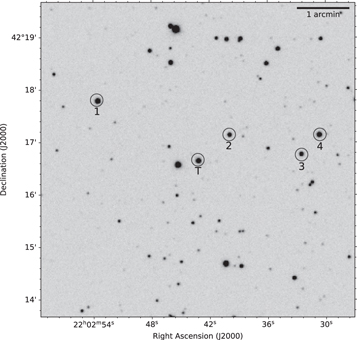
Figure 1. Finding chart of BL Lac in the R band. The labels "T" and "1–4" represent BL Lac, the comparison star, the check star, and two field stars, respectively.
Download figure:
Standard image High-resolution image3. The Light Curves
In Figure 2, the overall light curves of this source are displayed. BL Lac demonstrated clear interday variations during the period of our observation. The source was faintest on JD 2,458,792 with 0.81 mag in the R band and reached the brightest state on JD 2,458,746 with 0.30 mag. The total amplitude is <=1 mag. From visual inspection, we can find that these light curves are well correlated.
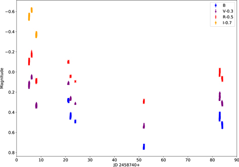
Figure 2. The overall B-, V-, R-, and I-band light curves of BL Lac.
Download figure:
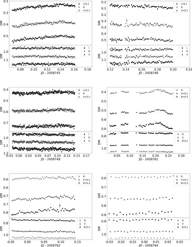
Standard image High-resolution imageThe intraday light curves of BL Lac are presented in the large panels in Figure 3. For clarity, the B-, V-, and I-band light curves are shifted by 0.3, 0.1, and 0.1 mag, respectively. In the small panels, the light curves of the check star are plotted, with the B band shifted by −0.1 mag.
Download figure:
Standard image High-resolution image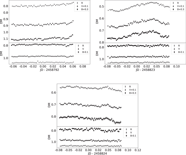
Figure 3. Intraday light curves. The large and small panels give the differential magnitudes (DMs) of BL Lac and the check star, respectively.
Download figure:
Standard image High-resolution imageBy visual inspection of the light curves, we can find IDVs of BL Lac on JDs 2,458,745, 2,458,761, 2,458,762, 2,458,792, 2,458,823, and 2,458,824. The object illustrated small-amplitude variations on these days. No sharp outburst was found. In combination with the shape of the overall light curves mentioned above, the object seems to be in a relatively quiescent state during the period of our observation.
4. IDV Detection
To quantitatively assess the existence of the IDV of the source, we adopted two statistical analysis techniques. They are the power-enhanced version of the F-test (de Diego 2014) and the analysis of variance (ANOVA; de Diego et al. 1998).
4.1. F-test
The original F-test (de Diego 2010) is implemented with a single check star, whose variance is compared with that of the target object, to obtain the statistical value F. In 2014, a power-enhanced version of the F-test was proposed by de Diego (2014). Because multiple field stars were considered, a higher degree of freedom will be generated and a more robust result will be produced. This test has been widely used in several recent IDV detections (e.g., Gaur et al. 2015; Polednikova et al.2016; Zhang et al. 2018).
In this test, we compared the variance of BL Lac to the combined variance sc 2 of the three field stars 2–4, which is defined as:

where Nj
is the number of observations of the jth field star and k is the number of field stars. The term  represents the scaled square deviation for the jth field star, and is defined as:

where ωj
is a factor to scale the variance of the jth field star to the same level of BL Lac (Howell et al. 1988), and mj,i
and  are the magnitude and mean magnitude of the corresponding light curve, respectively. The F is given by:

where sbll 2 is the variance of BL Lac. The final result includes two degrees of freedom (ν1 = N − 1 and ν2 = k(N − 1)) and F. They are listed in columns 6–8 in Table 1 and the critical values (Fc ) at the 99% confidence level are given in column 9. If F exceeds Fc , the null hypothesis will be rejected and the existence of variability (V) will be confirmed, otherwise we call it nonvariable (N).
4.2. ANOVA
ANOVA is a robust statistical test to detect the microvariations and is widely used in scientific researches (e.g., Polednikova et al. 2015; Meng et al. 2017; Zhang & Li 2017; Weaver et al. 2020; Butuzova 2021; Dai et al. 2021). The data in each individual differential light curve (DLC) are divided into k groups, with five data points in each group. The variance of groups is defined as:

where  is the average of the whole data set and yj
is the average of the jth group. The variance of the light curve is given by:
is the average of the whole data set and yj
is the average of the jth group. The variance of the light curve is given by:

where N is the number of the data points of the light curve. The F can be obtained by comparing the variance of groups to the variance of the light curve:

We adopted the same confidence level (99%) as in the F-test; if F exceeded Fc (listed in column 14), the light curve was taken as variable (V), otherwise it was nonvariable (N). F and two degrees of freedom of the ANOVA test are listed in columns 10–12 in Table 1. Meanwhile, we also applied the test to star 3 to avoid the detection of spurious variability, and the associated Fstar are listed in column 13 in Table 1. Only when both tests of BL Lac show "V" and the test of star 3 is "N" is BL Lac considered variable (V), otherwise it is nonvariable (N). The variability can be found in column 15 in Table 1.
Furthermore, an additional sanity check was applied to verify the robustness of ANOVA (Goyal et al. 2013; Pasierb et al. 2020). In our data set, a total of 81 steady star−star DLCs were involved. By applying ANOVA to these DLCs, the variability was detected on two and three DLCs at the significance level α = 0.01 and α = 0.05, respectively. Since the distribution of false positives is binomial, the expected number of false positives for ANOVA will be between 0 and 6 and in most cases between 0 and 2. At α = 0.05, the expected number of false positives for ANOVA should lie between 0 and 11 and in most cases between 2 and 6. The good agreement between the expected and the detected false positives proves the reliability of our analysis.
4.3. The Check for Seeing Disturbance
BL Lac is a relatively nearby object. Its emission is inevitably contaminated by its host galaxy light (e.g., Nilsson et al. 2018). If seeing variations were to play a role, the emission coming from the blazar and the host galaxy would be affected differently (Nilsson et al. 2007), and the observed brightness would appear to relatively brighten (dim) when the seeing is better (worse; Stalin et al. 2004). Therefore, it is crucial to assess whether the observed variations were dominated by a seeing change. One method would be to plot the FWHM variations of a comparison star for each night (Stalin et al. 2004; Goyal et al. 2007, 2009), which are presented in Figure 4. For clarity, the data points are sampled every 12 minutes. We did not find any obvious positive correlations between the variations of the brightness of BL Lac and the FWHMs, which demonstrates that the observed variations are intrinsic.

Download figure:
Standard image High-resolution image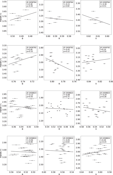
Figure 4. The FWHM−magnitude diagrams. The Pearson correlation coefficient r and the p value are given in the top right corner.
Download figure:
Standard image High-resolution image4.4. IDV Amplitude
We also calculated the IDV amplitude (Amp) for the light curves that are found to be variable. A widely used method to calculate Amp was proposed by Heidt & Wagner (1996):

where Amax and Amin are the maximum and minimum magnitudes, respectively, and σ is the measurement error. Occasionally, we need to deal with some faint objects associated with large errors; then, Amp will become 0 or even an imaginary number. So, we performed a mathematical modification with a Gaussian modulation function to the classical method. The amplitude can then be computed as

where Amax, Amin, and σ have the same definitions as in Equation (7). The validity of Equation (8) can be proved by a Taylor expansion. It is well known that  , and our modulation function can be written as:

If we only consider the first- and second-order Taylor expansion, Equation (8) will be equivalent to Equation (7). However, when σ increases, the third-order or even higher-order terms can no longer be ignored, and the two equations will gradually deviate from each other. To give an example, in Figure 5, we assumed a fixed  of 0.2 and plotted the variation of Amp versus the error (σ). The dashed and solid lines represent the Amp−error relation by the original and Gaussian modulated methods, respectively. When the error is small (∼0–0.06), there is almost no difference between the two methods. However, when the error gradually increases, the two curves gradually deviate from each other. The original method gives an amplitude of zero at an error of about 0.14, while the Gaussian modulated method can compute a reasonable amplitude at errors larger than ∼0.4. Although we did not find such large errors in our data, the modulation helps to enhance the robustness of the algorithm. In Table 1, column 16 gives our calculation of the IDV amplitude.
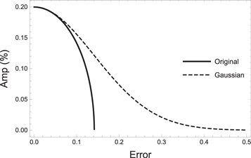
Figure 5. Amplitude−error diagram.  is fixed at 0.2. The dashed and solid lines represent the original method and the Gaussian modulated method, respectively.
Download figure:
Standard image High-resolution imageOver the nine nights, IDV was detected in all three bands on four nights and was not detected on the remaining five nights. Although the light curves on JD 2,458,762 showed obvious variability by visual inspection, we did not get any "V" on this night. This is perhaps due to the IDV exhibited also in the field stars. Furthermore, except for the results on JDs 2,458,745 and 2,458,761 (the amplitude of the I/R band is slightly larger than that of the R/V band), the variation amplitudes of BL Lac are monotonically increasing from the low-energy band to the high-energy band. In general, our results are consistent with those of previous studies, i.e., the higher the energy band, the greater the IDV amplitude (Webb et al. 1998; Meng et al.2017).
We noticed that IDVs were detected both in low and high states (see Figures 2 and 3). From the results of the long-term monitoring of the Katzman Automatic Imaging Telescope, 2 we found that BL Lac was in a rapid decay phase after a flare during our observations, and our starting epoch (JD 2,458,745) is around the flare maximum. Our results indicate that the detection of IDV is independent of the blazar's optical state. Similar phenomena occurred in some other blazars, e.g., PKS 0735+178 (Goyal et al. 2017), S5 0716+714 (Zhang et al. 2018), and 3C 273 (Liu et al. 2019).
5. Color Behavior
In this section, we investigated the color behavior with respect to the brightness of BL Lac for those nights when IDV was detected in all three bands. The color indices (CIs) of B − R, V − R, R − I, V − I, and B − R were calculated with the 5 min binned IDV data. Then we fitted the color–magnitude diagrams with a linear model and the results are displayed in Figure 6. The Spearman correlation coefficient (Sc) was calculated to estimate the significance of the correlation between the CIs and magnitudes.
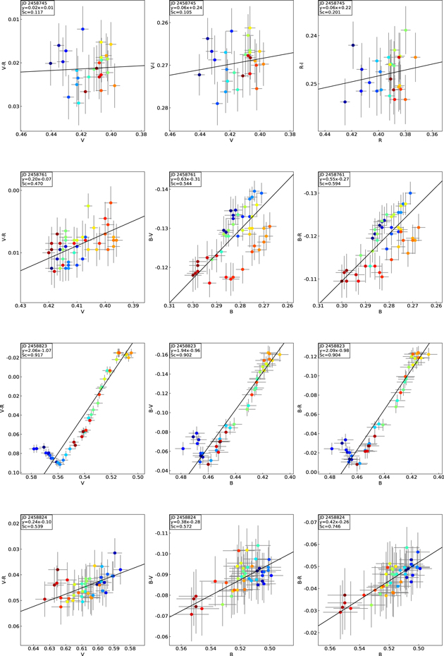
Figure 6. Color−magnitude diagrams of BL Lac. The epochs without IDV are excluded. The variations in color from cold to warm indicate the time sequence.
Download figure:
Standard image High-resolution imageExcept for the top three panels, all other diagrams exhibit a strong BWB trend. This color behavior is consistent with that found by previous studies (Racine 1970; Papadakis et al. 2007; Ikejiri et al. 2011; Gaur et al. 2015; Wierzcholska et al. 2015; Meng et al. 2017). On JD 2,458,823, although BL Lac showed an overall strong BWB trend, there were clear RWB heads in all three diagrams. The color behavior reversed at a certain brightness. These color reversals or saturations have been observed in a few FSRQs, e.g., 3C 279 (Isler et al. 2017), 3C 454.3 (Raiteri et al. 2008; Fan et al. 2018), and CTA 102 (Raiteri et al. 2017). As for BL Lac objects, only rare cases of a color reversal have been reported, e.g., AO 0235+164 (Safna et al. 2020; Wang & Jiang 2020) and PKS 0537−441 (Zhang et al. 2013). In fact, our case was the only one that occurred on the timescale shorter than one day.
Theoretically, the color behaviors of blazars include contributions from both the thermal emission of the accretion disk and the nonthermal emission of the relativistic jet. Since BL Lacs have radiatively inefficient accretion disks (Ghisellini & Celotti 2001; Ghisellini et al. 2009), it is reasonable to assume that the jet emission of BL Lac dominates over the disk emission most of the time. According to the jet emission model, the color behavior is significantly affected by the electrons' energy distribution (EED), i.e., a softer/harder injected EED than that of the cooled electrons leads to a RWB/BWB trend (Kirk et al. 1998; Mastichiadis & Kirk 2002). Such a color reversal suggests two components of injected EEDs on JD 2,458,823. In the low state, i.e., the state fainter than the broken magnitude in the fourth row in Figure 6, a softer injected EED resulted in the RWB trend. While in the high state, the injected EED hardened and resulted in the BWB trend. This hardening of the injected EED could be caused by the enhancement of the escape process. A large amount of electrons in the acceleration zone were not completely cooled and escaped from this region, and then were injected into the acceleration process (Kirk et al. 1998).
In previous studies, several models were proposed to explain the color reversal or saturation. The widely used one was the combined effect of a jet and some additional prominent components, e.g., the disk component or the broad emission line. Isler et al. (2017) illustrated that the observed color behavior depended on the ratio of the contributions of the accretion disk and jet, i.e., BWB/RWB was observed if the jet/disk component dominated the other one. A saturation state could be observed when the jet emission was comparable to the thermal emission from the disk. Such a saturation state has been observed in all of the FSRQs mentioned above (Raiteri et al. 2008, 2017; Isler et al. 2017; Fan et al. 2018), but has not been found in any BL Lac objects mentioned above. This is a natural result due to the radiatively inefficient accretion disk of BL Lac objects. In fact, all of the reported color reversals of BL Lac objects had the same color behavior, i.e., RWB in a low state and BWB in a high state. As a special BL Lac object, AO 0235+164 showed an evident component of an Mg ii line in the low state (Wang & Jiang 2020), and thus had an RWB trend. However, there was not enough evidence for the existence of a broad emission line in BL Lac. Our observations were most similar to the case of PKS 0537−441, for which Zhang et al.(2013) mentioned that EED was a key factor leading to such complex color behaviors. Moreover, the time lag is also a factor that may affect color behaviors (Wu et al. 2007). However, a color reversal requires two opposite time lags in the different active states, and it is obviously unphysical on a timescale shorter than one day.
In addition, the variations of the Doppler factor will also affect the color behaviors (Villata et al. 2002, 2004). Papadakis et al. (2007) demonstrated that the increase of the Doppler factor will blueshift the spectrum and result in a BWB trend. However, the short-term color behavior and especially the BWB trend are mainly attributed to the intrinsic processes related to the jet emission mechanism rather than to the geometrical reasons (Raiteri et al. 2013; Agarwal & Gupta 2015).
Moreover, we found two interesting color loops in the color–magnitude diagram on JD 2,458,761 and they can be seen in the last two panels of the second row in Figure 6. The data points trace clockwise loops in the B − V versus B and B − R versus B diagrams. 3 However, we did not find any clear such pattern in the V − R versus V panels. This spectral hysteresis has been observed in a few objects in X-ray (e.g., Sembay et al. 1993; Takahashi et al. 1996; Zhang et al. 1999, 2002; Kataoka et al. 2000) and in optical (e.g., Xilouris et al. 2006; Wu et al. 2007; Dai et al. 2013; Man et al. 2016; Pasierb et al. 2020). Thanks to our high precision and high temporal resolution data, it is the first time that such spectral hysteresis was observed in BL Lac. In general, different direction of the loop is expected depending on different relations between the acceleration and cooling timescales. A counter-clockwise loop is expected when the acceleration timescale is comparable to the cooling timescale. This is the so-called "hard lag". As for the clockwise loops found on JD 2458761, they are expected if the acceleration timescale is much shorter than the cooling timescale (Kirk et al. 1998). Such a clockwise loop is termed a "soft lag", i.e., the variations in low energies lag behind those in the high ones. We will verify this in the next section.
6. Time Lag
The spectral hysteresis suggests an interband time delay, which can be detected by a correlation analysis. We followed Grier et al. (2017) and performed the correlation analysis to measure the possible interband time lags by three different time-series analysis methods: the z-transformed discrete correlation function (ZDCF; Alexander 1997, 2013), the interpolated cross correlation function (ICCF; Peterson et al. 1998a), and JAVELIN (Zu et al. 2011). 4 The details of these methods are provided in each of these works. Here, we provide only a brief introduction of the settings we used in each method.
6.1. Settings
In ZDCF, the data points were binned into equal population bins and a Fishers z-transform was applied to stabilize the highly skewed distribution of the correlation coefficient. We obtained the ZDCF from the average of 1000 Monte Carlo (MC) realizations, and the time lag was then estimated by the accompanying algorithm named PLIKE (Alexander 2013), which calculates the maximum likelihood from the likelihood function, and the uncertainties were defined as the 68.2% fiducial interval of the normalized likelihood function.
ICCF combined a linear interpolation and a cross correlation analysis to estimate the time lags, and our procedure was implemented through the publicly available PyCCF (Peterson et al. 1998b) algorithm. 5 The settings are as follows.
- 1.We computed the ICCF with a grid spacing of 0.3 min.
- 2.A total of 10,000 MC realizations were employed and a cross correlation centroid distribution (CCCD) was adopted.
- 3.The cutoff correlation coefficient was set to be r0 = 0.5. In each MC realization, the maximum correlation coefficient should satisfy
 , otherwise this MC will be marked as "failed" and the result will not be recorded. The failure rates (the ratio of failed MC times to total MC times) are listed in column 3 of Table 2.

Table 2. Results of Cross Correlation Analysis
| Date | Bands | Failure Rate | rmax | ZDCF | ICCF | JAVELIN |
|---|---|---|---|---|---|---|
| (JD) | (%) | lag (min) | lag (min) | lag (min) | ||
| 2,458,745 | V − R | 0 | 0.87 |

|

|

|
| V − I | 0 | 0.88 |

|

|

| |
| R − I | 0 | 0.84 |

|

|

| |
| 2,458,746 | V − R | 82.5 | 0.52 |

|

|

|
| V − I | 56.3 | 0.50 |

|

|

| |
| R − I | 47.9 | 0.58 |

|

|

| |
| 2,458,761 | V − R | 0 | 0.94 |

|

|

|
| B − V | 0 | 0.83 |

|

|

| |
| B − R | 0 | 0.85 |

|

|

| |
| 2,458,762 | V − R | 43.7 | 0.53 |

|

|

|
| B − V | 13.6 | 0.79 |

|

|

| |
| B − R | 34.0 | 0.59 |

|

|

| |
| 2,458,792 | V − R | 0.3 | 0.81 |

|

|

|
| B − V | 9.8 | 0.78 |

|

|

| |
| B − R | 12.4 | 0.77 |

|

|

| |
| 2,458,823 | V − R | 0 | 0.97 |

|

|

|
| B − V | 0 | 0.95 |

|

|

| |
| B − R | 0 | 0.94 |

|

|

| |
| 2,458,824 | V − R | 0 | 0.89 |

|

|

|
| B − V | 0.7 | 0.86 |

|

|

| |
| B − R | 0.1 | 0.90 |

|

|

|
Note. The columns show the observational Julian Date, the bands, failure rate, the maximum correlation coefficient in PyCCF, the measured lag of ZDCF, ICCF, and JAVELIN, respectively. Positive values indicate that the previous band leads the latter one.
Download table as: ASCIITypeset image
We also computed the lags using the JAVELIN algorithm (Zu et al. 2011), which assumed a damped random walk model to interpolate the driving light curve at unmeasured times. Another light curve was treated as a scaled, shifted, and smoothed version of the driving light curve by simultaneously fitting a top-hat transfer function using Markov Chain Monte Carlo (MCMC) techniques. After 10,000 iterations of MCMC, we obtained the posterior distributions (PDs) of the time lag. Due to a multiple peak alias in the CCCD/PD, the specific time lag and uncertainties are estimated after an alias removal. In the above three algorithms, we empirically searched those lags smaller than ±60 min.
In addition, we applied an alias removal algorithm to address the multipeak alias in the CCCD/PD. This algorithm combined a weighted lag distribution and a smooth operation through the kernel density estimate (KDE) to determine the most likely peak that provides the true time lag. The detailed procedure can be seen in Grier et al. (2017). The bandwidth of the Gaussian kernel we used in the KDE was 0.25 min. We finally chose the median and 16th/84th percentiles of the most likely peak as the time lag and lower/upper limit, respectively. Figure 7 shows examples (JD 2,458,745) of time lags measured with the three methods. The complete results are shown in Table 2. It is worth mentioning that the average failure rate on JDs 2,458,748 and 2,458,764 reached 96% and 99%, respectively, so the results on these two epochs are not presented in Table 2.

Figure 7. Examples of lags measured with three methods on JD 2,458,745. The left, center, and right panels represent the V − R, V − I, and R − I lags, respectively. The measured lags and uncertainties are given in all panels and are indicated by the solid and dotted lines, respectively. Top panels: the discrete correlation coefficient (points) and the likelihood (curves) obtained from ZDCF and PLIKE, respectively. Bottom two rows: the CCCD and PD obtained from PyCCF and JAVELIN, respectively. The dashed lines indicate the KDE of the weighted CCCD/PD and the histograms are the unweighted CCCD/PD. The shaded regions highlight the ranges of lags included in the final calculation.
Download figure:
Standard image High-resolution image
6.2. Results
As shown in Table 2, three reliable time lags were measured in the BV and BR bands on JD 2,458,761 and in the BR band on JD 2,458,823. Except for a failure rate of 0 and an rmax over 0.8, all three methods give nonzero measurements that are basically consistent with each other within the error range, which indicates the existence of a real time lag. The former two lags verified the spectral hysteresis on JD 2,458,761, and the time lags were finally chosen as ∼16 and ∼18 min (approximately the average of the three measurement results) in the B − V and B − R bands, respectively. Due to the high failure rate on JD 2,458,746 and 2,458,762, most of the measured lags were inconsistent with each other and even showed a time lag near the search boundary, which is a sign of a false measurement (Yang et al. 2020).
Almost all of the remaining measurements give a near-zero time lag, which is very common on both long-term and short-term timescales (e.g., Wu et al. 2007; Man et al. 2016; Grier et al. 2017; Mudd et al. 2018; Zhang et al. 2018; Grier et al. 2019). This is because the electrons lose their energy through synchrotron radiation, and the higher-energy electrons lose energy faster than those lower-energy ones (Marscher & Gear 1985). This leads to the time lags toward lower frequencies. However, different optical bands have only small wavelength separations and it is difficult to detect the time lags between the optical bands.
As mentioned by Wu et al. (2012), whether a reliable time lag could be detected depends on four key factors: (1) wavelength separation, (2) variation amplitude, (3) temporal resolution, and (4) measurement accuracy. The wavelength separation is proportional to the probability that a reliable lag can be detected. For the second factor, a reliable time lag was usually derived in those blazars with large variation amplitudes. However, it is not always true. Assuming two monotonically brightening/darkening light curves, they may have a large variation amplitude, but due to the lack of other features (e.g., a complete flare that contains a rising phase and a decaying phase), it is still possible to detect a near-zero lag, just as we have observed on JD 2,458,745. Since the interband time lags between optical bands could be as short as a few minutes, a temporal resolution of less than 5 min is favorable. For the fourth, high accuracy is helpful to detect a reliable time delay, and thus a relatively bright target source and comparison star should be chosen.
7. Summary
We observed BL Lac in the B, V, R, and I bands with the 85 cm telescope at the Xinglong Observatory of the NAOC from 2019 September 18 to 2019 December 6 and collected 2305 data points on nine nights. The variations were well correlated in all bands. BL Lac was faintest on JD 2,458,792 with 13.42 mag and reached the brightest state on JD 2,458,746 with 12.94 mag in the R band.
We focused on the IDV of BL Lac. IDV was detected in all three bands on four nights. There is no IDV on the remaining five nights. Moreover, we upgraded the classical IDV amplitude algorithm to incorporate possible large errors in photometric measurements and found greater IDV amplitudes in higher-energy bands.
The BWB trends were found on all nights with IDV. A color reversal was found on JD 2,458,823, which is the first observed in BL Lac objects on an intraday timescale. This indicates that there are two different energy distributions of injected electrons on this night. It may provide a reference for analyzing the complex emission mechanisms of BL Lac objects. Moreover, a clockwise loop was found on the color–magnitude diagram of JD 2,458,761, which indicates that the acceleration timescale of BL Lac is much shorter than its cooling timescale (Kirk et al.1998).
The most reliable measurements of time lags appear on JD 2,458,761 and are ∼16 and ∼18 min in the BV and BR bands, respectively. Such a "soft lag" is in accord with the clockwise loops. This adds one more case to the few optical interband lags that are reported in recent years (e.g., Wu et al. 2007; Dai et al. 2013; Man et al. 2016).
Footnotes
- 1
IRAF is distributed by the National Optical Astronomy Observatories, which are operated by the Association of Universities for Research in Astronomy, Inc., under cooperative agreement with the National Science Foundation.
- 2
- 3
Two color loops were also presented in the V − R versus V and V − I versus V diagrams on JD 2,458,745. However, their variations were not chronological.
- 4
- 5