


Abstract
In this work, we present the results of the survey carried out on one of the deepest X-ray fields observed by the XMM-Newton satellite. The 1.75 Ms Ultra Narrow Deep Field (XMM175UNDF) survey is made by 13 observations taken over 2 yr with a total exposure time of 1.75 Ms (1.372 Ms after flare-filtered) in a field of 30' × 30' centered around the blazar 1ES 1553+113. We stacked the 13 observations reaching flux limits of 4.03 × 10⁻¹⁶, 1.3 × 10⁻¹⁵, and 9.8 × 10⁻¹⁶ erg s−1 cm−2 in the soft (0.2–2 keV), hard (2–12 keV), and full (0.2–12 keV) bands, respectively. Using a conservative threshold of Maximum Likelihood significance of ML ≥ 6, corresponding to 3σ, we detected 301 point-sources for which we derived positions, fluxes in different bands, and hardness ratios. Thanks to an optical follow-up that was carried out using the 10.4m the Gran Telescopio Canarias on the same field in the u'g'r'i'z' bands, combined with WISE/2MASS IR data, we identified 244 optical/IR counterpart candidates for our X-ray sources and estimated their X-ray luminosities, redshift distribution, X-ray/optical–X-ray/IR flux ratios, and absolute magnitudes. Finally, we divided this subsample into 40 non-active sources and 204 active galactic nuclei, of which 139 are classified as Seyfert galaxies and 41 as Quasars.
Export citation and abstract BibTeX RIS
1. Introduction
One of the biggest problems in cosmology is understanding the connection between Super Massive Black Holes (SMBHs) and Galaxy formation (Merritt 2000; Di Matteo et al. 2005; Done 2010). To uncover this co-evolution, it is necessary to detect and characterize large samples of Active Galactic Nuclei (AGNs) and their hosts using multiwavelength analysis through larger and deeper surveys in a variety of bands, such as optical, infrared, radio, and X-ray (Scoville et al. 2007; Kellermann et al. 2008; Rosen et al. 2016; Brandt & Vito 2017). AGNs are galaxies that host an accreting SMBH in their nuclear region, which emits a large amount of X-ray photons via accretion processes (George & Fabian 1991; Haardt & Maraschi 1991; Matt et al. 1997). Contrary to optical and infrared surveys, which may suffer incompleteness and/or misidentification problems (e.g., Scoville et al. 2007), X-ray surveys provide a very powerful tool to blindly search for AGNs (Brandt & Alexander 2015). Additionally, (1) X-ray emission can penetrate through high column densities of material (NH = 1021–1024.5 cm−2), which allows the detection of moderately obscured AGNs (Ghisellini et al. 1994; Ghosh et al. 2008; Hickox & Alexander 2018); (2) X-ray emission of AGNs suffers low dilution by their host galaxy as opposed to radiation in the optical band; and (3) X-ray spectra of AGNs can be used as a diagnostic tool to infer luminosity, obscuration level, nuclear geometry, disk/corona conditions, and Eddington ratio (LBol/LEdd) (Brandt & Vito 2017). Therefore, X-ray surveys allow us to identify large samples of obscured (Log NH > 21.5 cm−2) and unobscured AGNs, which makes it possible to study their contribution to the Cosmic X-ray Background (XRB) that is associated to the integrated X-ray emission from extragalactic faint point sources (Gilli et al. 2007).
In the last two decades, X-ray missions such as XMM-Newton and Chandra have performed shallow X-ray surveys over wide fields and deep surveys in narrow areas (for a detailed summary, see Brandt & Alexander 2015). The strategy of surveying large areas is to look into large volumes of the universe, which increases the probability of finding high-luminous QSOs and atypical sources that could be missed by small coverage surveys (Evans et al. 2010; Warwick et al. 2012; Rosen et al. 2016). In contrast, deep X-ray surveys in narrow field areas are an effective method to identify moderately luminous AGNs and faint high-redshift sources (Brusa et al. 2007; Puccetti et al. 2009; Marchesi et al. 2016; Vito et al. 2016).
The X-ray observations that are analyzed here were originally dedicated to study the Warm Hot Intergalactic Medium (WHIM) with the goal of observing highly ionized intervening absorbers via detection of O vii features in the spectrum of the blazar IES 1553+113 (Nicastro et al. 2018; Das et al. 2019).
This project gathered in 2 yr a total of 13 observations targeting the blazar and the 30' × 30' area around it, generating a total exposure time of 1.75 Ms. As a by-product, this program created the 1.75 Ms Ultra Narrow Deep Field (XMM175UNDF), which is one of the narrowest and deepest surveys ever performed with XMM-Newton in the band 0.2–12 keV and is particularly well-suited to survey the AGN content of the field.
To search for optical counterparts and provide solid photometric and spectroscopic identifications, we performed an optical campaign of this field with the OSIRIS camera mounted at the 10 m Gran Telescopio Canarias (GTC). Finally, we cross-correlated our X-ray/optical catalog with available infrared (IR) coverage by WISE/2MASS from Cutri et al. (2014).
In this paper we present a catalog of 301 X-ray point-sources, 9 which is consistent with the results obtained for this field by the XMM-Newton Survey Science Centre and recently reported by Webb et al. (2020), Traulsen et al. (2020).
This paper is organized as follows. In Section 2, we present the XMM-Newton observations and procedures for data reduction. We describe the method used to identify the X-ray sources and the details of the production of the X-ray point-source catalog and its statistical reliability. In Section 3, we identify the optical/IR counterparts by cross-matching the X-ray catalog with the optical/IR catalogs, using the Likelihood Ratio (LR) technique and we explain our photo-z determination procedure. In Section 4, we describe the general properties of the X-ray catalog and the Log N–Log S data analysis. In Section 5, we present the results of our multiwavelength analysis (e.g., luminosity distribution, AGN identifications). In Sections 6 and 7, we discuss and summarize the most important results of the paper. Throughout this work, we adopted the cosmological parameters H0 = 70 km s−1 Mpc−1, Ωm = 0.3 and ΩΛ = 0.7.
2. Data Processing and Source Detection
The present XMM-Newton survey comprises 13 observations taken in 2015 and 2017 covering an area of 30' × 30' centered at the blazar 1ES 1553+113 (R.A. = 238°55'45 48, decl. = 11°11'2436) (Nicastro et al. 2018). The stacked exposure time for the 13 observations is 1.75 Ms. We processed the EPIC (PN, MOS1, and MOS2) data of our observations with the XMM-Newton Science Analysis Software version 17 (SAS, Gabriel et al. 2004). More specifically, for each EPIC observation, we used the package epicproc (epproc, emproc) to process the data, extract images, and light curves.
Observations were then filtered for periods of high background caused by soft protons, as follows: first, we used the tool evselect to create source-free 10–12 keV background light curves (with bin size of 100s), for each observation and for each available instrument. Then, we employed the task bkgoptrate in those light curves to identify the optimum background rate cut threshold which maximizes the signal-to-noise ratio (S/N) for a given background. 10 We found that the six observations that were taken in 2015 show a much lower background compared to the seven that were observed in 2017 (77 ks of PN high background removed in 2015 versus 296 ks in 2017). The final exposures are 1.372, 1.56, and 1.511 Ms for PN, MOS1, and MOS2, respectively (see Table 1).
Table 1. Resume of XMM-Newton Observations Around the Blazar 1ES 1553+113
| Obs.ID | Date | Nominal Exp | Exp Clean PN | Exp Clean MOS1 | Exp Clean MOS2 | Distance |
|---|---|---|---|---|---|---|
| (ks) | (ks) | (ks) | (ks) | (arcmin) | ||
| 761100101 | 2015 Jul 29 | 138.4 | 126.3 | 128.5 | 133.6 | 0.5 |
| 761100201 | 2015 Aug 2 | 138.9 | 122.1 | 130.4 | 128.6 | 0.24 |
| 761100301 | 2015 Aug 4 | 138.9 | 133.4 | 131.5 | 135.5 | 0.25 |
| 761100401 | 2015 Aug 8 | 138.9 | 120.6 | 130.2 | 126.9 | 0.49 |
| 761100701 a | 2015 Aug 16 | 90 | 85.4 | 85 | 87.8 | 0 |
| 761101001 | 2015 Aug 30 | 139 | 119.2 | 132.9 | 128.5 | 0 |
| 790380501 | 2017 Feb 1 | 143.2 | 33 | 65.5 | 54.5 | 0.5 |
| 790380601 | 2017 Feb 5 | 143.2 | 86.6 | 117.92 | 100.3 | 0.25 |
| 790380801 | 2017 Feb 7 | 143.2 | 101.2 | 131.9 | 114.6 | 0.25 |
| 790380901 | 2017 Feb 11 | 143.2 | 118 | 137 | 133.8 | 0.5 |
| 790381401 | 2017 Feb 13 | 145.7 | 112.4 | 140.1 | 132.9 | 0 |
| 790381501 | 2017 Feb 15 | 145.7 | 136.6 | 139.4 | 140.2 | 0.5 |
| 790381001 a | 2017 Feb 21 | 97 | 77.7 | 90.5 | 93.4 | 0 |
| TOTAL | 1750 ks | 1372 ks | 1560 ks | 1511 ks | ||
Notes. The distance in the last column is measured in arcminute from the center of each observation to the blazar.
a PN small-window observation.Download table as: ASCIITypeset image
2.1. Stacked Source Detection
For the process of source detection on the stacked images, we used the new standardized XMM-Newton approach with the new task edetect_stack, 11 considering the same parameters and the five standard energy bands (0.2–0.5, 0.5–1, 1–2, 2–4.5, 4.5–12 keV) as in the 3XMM and 4XMM catalogs (Rosen et al. 2016; Traulsen et al. 2020; Webb et al. 2020). The task edetect_stack was prepared to perform standardized EPIC source detection on individual and overlapping fields of observations taken at different epochs. This task includes runtime improvements and comprises 12 stages, which are run subsequently. In every stage, it creates and uses in parallel data products as coupling images, exposure maps, background maps, and detection masks for each observation, instrument, and energy band (for more details, see Traulsen et al. 2019).
2.2. Stacked Source List and Maximum Likelihood Fitting
The task edetect_stack runs emldetect to calculate the X-ray source parameters of the catalog (fluxes, count rates, source counts, Maximum Likelihoods, hardness ratios) in each band for the PN, MOS1, and MOS2 cameras by fitting the instrumental PSF convolved with the source counts distribution in each energy band and camera (Hasinger et al. 1993). Meanwhile, emldetect computes the likelihood significance L for each source by observation and energy band. L is defined as in Cruddace et al. (1988), Hasinger et al. (1993)

where p is the probability of Poissonian random fluctuation of the counts in the detection cell, which is calculated using the incomplete Gamma function Γ as a function of raw source counts and raw background counts in the detection box. The detection likelihoods Li for each observation are converted to Maximum Likelihoods (ML), with two free parameters equivalent to perform a detection run on a single image
where ν is the number of degrees of freedom of the fit (ν = 2 + n, n as the number of energy bands). To minimize spurious source content, the detection likelihood is derived for each source using the best-fit C-statistic (Cash 1979), minimizing the deviation between measured counts c and the model prediction m in a region of N pixels
where ci = cs + cb is the sum of source counts cs and background counts cb in the detection region, mk is the model prediction; as a result, Li can be characterized as Li = Ci (ci ) − Ci (cb ). Since every observation is centered around the blazar 1ES 1553+113 (F0.2−12 keV ≃ 2 × 10⁻¹¹ erg s−1 cm−2), we decided to set a circular mask of 3' radius centered on 1ES 1553+113 to avoid false identifications of sources, due to the star-like pattern created by the spider structure which supports the mirrors of the telescope (see Figure 1).
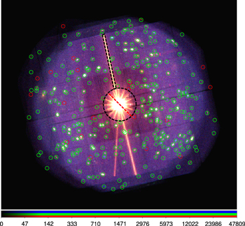
Figure 1. Composite mosaic image of all observation of the survey at three different bands: 0.2–1 keV (red), 1–2 keV (green) and 2–12 keV (blue). Green circles mark the 301 X-ray point-like sources detected in our final source list. Red circles mark a subsample of 19 objects detected in only one pointing. The circular and rectangular black doted regions mask the blazar 1ES 1553+113 and the out of time events, respectively. The color bar is in counts.
Download figure:
Standard image High-resolution image2.3. Source Selection Process and Final Source List
We set a conservative detection threshold of ML ≥ 6, corresponding to a Poisson probability of p ≃ 2.5 × 10⁻³ (i.e., 3σ). Consequently, we found 483 X-ray sources, of which 49 are classified as extended. Since most of our extended sources were detected along stray lights and along remaining residuals of the masked region around the blazar, we limited our analysis to the point-like sources.
We then proceeded to an accurate visual inspection of each source of our catalog in the final stacked image, and we were able to identify 59 additional spurious detections that appeared only in one observation and/or along stray-light strips or correspond to hot pixels, which we therefore removed from our analysis.
Finally, we also excluded 74 additional X-ray sources, which were detected only in the MOS1 camera and correspond to instrumental artifacts. Our final X-ray catalog contains 301 sources, all of which were at least detected in the PN camera, of which six were detected only in one band, while 38 sources were detected in two bands.
2.4. Comparisons with 4XMM Catalogs
To support the reliability of our results, we carried out a comparison with the most recent data release produced by XMM-Newton Survey Science Centre (SSC): 12 the 4XMM catalogs of serendipitous sources from individual (Webb et al. 2020, hereafter DR9) and overlapping (Traulsen et al. 2020, hereafter DR9s) fields. Both catalogs used the same 13 observations that we presented in this paper plus 10 PN small-window calibration observations (each of ∼30 ks). The main difference between our work and theirs consists in the fact that these two catalogs were obtained by an automated process, whereas our analysis optimizes the data reduction and source detection as follows: we masked the regions affected by the contribution of the very bright source at the center of the images and the out of time events; we maximized the S/N in our cleaned observations; and we drastically reduced the number of spurious detections by removing bright pixels, detector features/artifacts and detections in the PSF spikes of bright sources.
In Appendix A, we present the detailed comparison analysis of our catalog versus DR9s and DR9 catalogs. Overall, we found a good consistency between both catalogs and our results: we found 288 (DR9s) and 284 (DR9) common sources within our final catalog of 301 objects.
3. Optical/IR Dataset and X-Ray Counterparts
3.1. Optical Observations and Infrared Catalog
The optical catalog that is used in this work was produced with observations from the OSIRIS 13 camera at the 10 m Gran Telescopio Canarias (GTC), as a result of a campaign carried out on the same XMM-Newton field (PI Krongold, Nicastro et al. 2018). Four-by-four mosaic observations were performed with the Sloan Digital Sky Survey (SDSS) magnitude filters u'g'r'i'z' centered at 350, 481.5, 641, 770.5, and 969.5 nm, respectively. The optical detections have S/N = 3 down to magnitude limits of 23.3, 24.9, 24.4, 23.9, and 22.7, while for faint detections with S/N = 2 we used the Upper Limit (UL) of 23.7, 25.3, 24.8, 24.3, and 23.1, respectively.
The optical data were reduced with IRAF using the gtcmos package (Gómez-González et al. 2016), while for the source detection process we used SExtractor. Our analysis produced an optical catalog of 43,068 objects. We computed their fluxes using the SDSS photometry in AB system. 14
The infrared catalog was taken from a public repository of the Wide-field Infrared Survey Explorer (WISE) (Wright et al. 2010), which additionally presents 2MASS counterparts. To cover the full XMM175UND-Field of ≈28 arcmin2, we used a search cone of 20' radius centered on the blazar 1ES 1553+113 with the software topcat. 15 We obtained an IR catalog of 5849 WISE sources detected at S/N > 5 in the W1, W2, W3, and W4 mid-infrared WISE bands centered at wavelengths of 3.4, 4.6, 12, and 22 μm (Cutri et al. 2014), of which 898 sources present 2MASS counterparts in the near-infrared J, H, and Ks bands. We computed the 2MASS Ks-band fluxes at 2.17 μm when available, for the remaining sources we used the WISE W1-band corrected by the empirical relation Ks = 0.99 × W1 + 0.23 (Cluver et al. 2014).
3.2. Optical/Infrared Counterparts and Likelihood Ratio Technique
The optical and infrared identifications for the X-ray sources were obtained by using the likelihood-ratio technique (Sutherland & Saunders 1992) considering a significance of 3σ (Brusa et al. 2007, 2010; Ranalli et al. 2013; Luo et al. 2017; Chen et al. 2018). We used the likelihood-ratio technique as described in Pineau et al. (2011), using the plugin Xcorr developed within Aladin. The likelihood ratio (LR) is defined as the ratio between two probability densities (see Equation (6)): first, the probability to have a real association counterpart

and second, the probability that the identification is due to background fluctuations

Therefore, LR has the expression:
where  and
and  . d is the angular distance that separates both sources, σX
(X-ray) and σO
(optical or infrared) are the positional error and N(m) is the angular density of objects with magnitude m (for more details, see Pineau et al. 2011).
. d is the angular distance that separates both sources, σX
(X-ray) and σO
(optical or infrared) are the positional error and N(m) is the angular density of objects with magnitude m (for more details, see Pineau et al. 2011).
The X-ray source positional error used in our sample is defined as:

This was obtained by the quadrature combination of the systematic positional error SYSERRCC due to systematic uncertainties (e.g., pointing uncertainties and cross-calibration in the stacked observations) and the statistical positional error RADEC_ERR, which is defined as:

Where σα
and σδ
are the 1σ errors on the image coordinates. For our analysis we considered a mean systematic error SYSERRCC = 043. This value was taken from Traulsen et al. (2019), who compared the position offsets of a catalog of 71,951 unique X-ray sources (from 1789 overlapping XMM-Newton observations) and a set of associated Quasars from SDSS-DR12 (see Traulsen et al. 2019, Figure 15). Consequently, we obtained a mean source X-ray positional error POSERR = 066 ± 0.25.
We found 244 X-ray sources with at least an optical or infrared counterpart association (81% of the X-ray sources), of which 137 present both optical and IR counterparts, 90 only optical and 17 only IR counterparts (e.g., 227 optical and 154 IR counterparts). To illustrate a few examples of those objects, in Figure 2 we present a set of XMM-Newton and GTC (in r band) images of 6 X-ray sources with their corresponding optical counterparts.
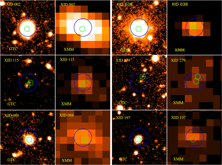
Figure 2. Example of 6 XMM-Newton randomly selected X-ray sources with their respective GTC optical counterparts in  band images. In each chart, the green circles with a radius of 15 mark the position of the optical counterpart sources, the blue circles with a radius of 5'' are centered on the XMM-Newton position. Every box is
  across.
Download figure:
Standard image High-resolution imageIn Figure 3, we plot the angular separation distribution in arcseconds, resulting from the cross-correlation of the X-ray with GTC and WISE sources, which yielded a median angular separation of σ = 103 and σ = 121, respectively. For sources that are associated with two optical counterparts (22), we considered the one with highest LR for further analysis (see Appendix C Table 6).
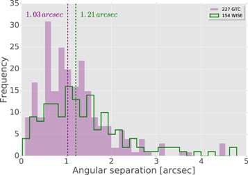
Figure 3. Angular distance distribution for GTC (227, purple filled) and WISE (154, green unfilled) counterpart candidates, respectively, as a result from the cross-correlation procedure by Xcorr.
Download figure:
Standard image High-resolution image3.3. Spectroscopic and Photometric Redshift
The photometric redshifts were obtained with PhotoRApToR, a tool for photo-z calculation based on the machine-learning model MLPQNA (Multi Layer Perceptron trained by the Quasi Newton Algorithm) (Cavuoti et al. 2015).
PhotoRApToR uses a modern algorithm based on a neural network that was trained by using only the spectra of sources detected within our optical catalog, with the aim to execute a well-controlled experiment. The sources used for training the code present the following advantages: (1) they are observed with the same instruments, optical bands, and observing conditions; and (2) they were detected in the same field (i.e., equal Galactic absorption).
An advantage of this method is that the algorithm does not require classical galaxy templates, and therefore it is not affected by its limitations (e.g., some sources that may be difficult to characterize). Moreover, thanks to the fact that most of our training set is composed by emission-line galaxies rather than absorption line objects (see Appendix B), our code is optimized to detect and estimate the photo-z of emission-line sources. Therefore, because we expect that most of our X-ray AGNs with spec-z are emission-line objects, we are confident that our photo-z estimations are statistically corrected.
3.3.1. The Training Sample
We used a set of 824 sources with good spectroscopic redshifts quality observed in the XMM175UND-Field. This spec-z catalog is a combination of a recent observational campaign by Johnson et al. (2019) with 762 objects with  mag limit, 29 from SDSS DR16 (Ahumada et al. 2020) with
  and 33 sources from our own GTC-Osiris spectroscopic observations with
  . In Appendix B, we show the procedure executed for the analysis of these 33 optical spectra.
Additionally, 39 sources of our X-ray catalog have an optical counterpart association with our spec-z catalog. In total, 32 of them were included in the training set template to estimate the photo-z and the remaining seven are in the test set, which may improve our results in terms of accuracy. We trained the neural network by using the five optical bands  as the input parameters with an 80% (659) of our spec-z catalog as the training set, leaving the remaining 20% (165) to test our results (see Figure 4). Since 99% of the sources of our spec-z catalog have redshifts in the zspec = 0–1.5 range, we could constrain our photo-z in a reliable way up to z ∼ 1.5.
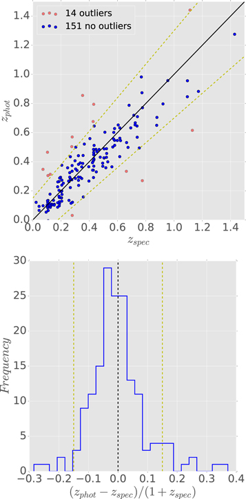
Figure 4. Upper panel: Photometric vs. spectroscopic redshifts distribution for our test sample composed by 165 (20%) sources from our spec-z catalog. Lower panel: residual histogram between the photo-z and the spec-z. The black-solid line in both plots represents the ideal case when zspec = zphot, and the dashed yellow lines limit the confidence region ∣zspec − zphot∣ < 0.15 × (1 + zspec) for outliers (red-solid points).
Download figure:
Standard image High-resolution imageThen, we used the normalized median absolute deviation (NMAD) defined as σNMAD = 1.4826 × Median(Δz/(1 + zspec)) as an indicator of the quality of our photo-z estimation, where Δz = ∣zspec − zphot∣. We found an accuracy of σNMAD = 0.062 with ∼8.5% (14) of outliers (e.g., ∣zspec − zphot∣ > 0.15 × (1 + zspec)) and a normalized standard deviation σΔz/(1+z) (or σnorm) of 0.064. Our results are comparable with previous works such as the XMM-Newton survey in the COSMOS field (σnorm = 0.05, outliers ≈8%, Brusa et al. 2007, 2010), and the XMM-SERVS survey (σNMAD = 0.040, outliers = 8.7%, Chen et al. 2018).
To test the effect of the number of added X-ray sources to the training set (82% in the analysis above), we trained our neural network considering two additional cases: using a training set without X-ray objects and with 50% of them (20 out of 39). We found a fraction of 8.4% of outliers with σNMAD = 0.0634 for the first case. For the second case we found 8.6% of outliers with σNMAD = 0.0625. These results show that there is no dependence with the number of X-ray sources used in the training set. We stress again that this is because most of our spectroscopic sample consists of objects with emission lines.
After performing our photo-z calculation and considering the spectroscopic sample, we achieved a ∼93% (211 out of 227) of redshift completeness for our X-ray sources with optical counterparts. In Figure 5, we show the histograms for our photometric (red), spectroscopic (blue) and full (white) redshift distribution of our X-ray sources in the XMM175UND-Field.
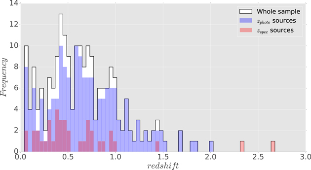
Figure 5. Redshift histogram of 211 sources of our X-ray catalog with zspec/zphoto estimations (white bars) with a bin size of 0.04. The blue and red bars, respectively, represent the photo-z (172) and spec-z (39) sources.
Download figure:
Standard image High-resolution image4. X-Ray Source Properties
4.1. X-Ray Flux Distribution
The final X-ray catalog consists of 301 objects, of which 87 are detected only in the soft bands (0.2–0.5, 0.5–1, 1–2 keV), 17 only in the hard bands (2–4.5, 4.5–12 keV) and 197 are detected simultaneously in both soft and hard bands. These 197 objects are defined as "sources detected in the Full band (0.2–12 keV)" (see Table 2).
Table 2. Summary of X-Ray Source Counts by Energy Band in Our XMM175UNDF Catalog
| Band | Ntot a | Ntot,obs b | Nfil c | Nfil,obs d |
 e
e
|
|---|---|---|---|---|---|
| (keV) | (10−15) cgs | ||||
| 0.2–0.5 | 148 | 0.07 | 148 | 0.07 | 0.16/14.75 |
| 0.5–1 | 212 | 0.13 | 205 | 0.12 | 0.20/30.97 |
| 1–2 | 262 | 0.26 | 251 | 0.27 | 0.25/45.11 |
| 2–4.5 | 212 | 0.35 | 205 | 0.33 | 0.76/68.37 |
| 4.5–12 | 82 | 0.35 | 81 | 0.35 | 3.63/145.59 |
| Soft | 282 | 0.25 | 269 | 0.26 | 0.4/90.45 |
| Hard | 212 | 0.35 | 205 | 0.33 | 1.3/213.96 |
| Full-band f | 197 | 0.3 | 196 | 0.3 | 0.98/304.41 |
| Only Soft g | 87 | ⋯ | 75 | ⋯ | 0.4/5.91 |
| Only Hard h | 17 | ⋯ | 11 | ⋯ | 3.43/36.7 |
| Full-Survey i | 301 | 0.3 | 282 | 0.29 | 0.98/304.41 |
Notes. The first five bands are the standard detection bands (Rosen et al. 2016), the following two bands are for sources detected in the soft and hard bands, respectively.
a Total sources detected by band. b Fraction of obscured sources (HR ≥ − 0.2) (see Section 4.3) of Ntot. c Final number of filtered sources to compute the distribution.
d
Fraction of obscured filtered sources (see Sections 4.2.1 and 4.2.2 for details).
e
Minimum and maximum fluxes per band in erg cm−2 s−1 assuming a Γ = 1.7 corrected for Galactic absorption.
f
Sources detected simultaneously in the soft and hard band.
g
Sources detected in the soft band but not in the hard band.
h
Sources detected in the hard band but not in the soft band.
i
0.2–12 keV band for sources detected at least in one of the standard detection bands.
distribution.
d
Fraction of obscured filtered sources (see Sections 4.2.1 and 4.2.2 for details).
e
Minimum and maximum fluxes per band in erg cm−2 s−1 assuming a Γ = 1.7 corrected for Galactic absorption.
f
Sources detected simultaneously in the soft and hard band.
g
Sources detected in the soft band but not in the hard band.
h
Sources detected in the hard band but not in the soft band.
i
0.2–12 keV band for sources detected at least in one of the standard detection bands.Download table as: ASCIITypeset image
Similar to other XMM-Newton catalogs created by the SSC (Rosen et al. 2016; Traulsen et al. 2019, 2020; Webb et al. 2020), we estimated our source fluxes using the same count-to-flux conversion factors adopted by Mateos et al. (2009). The model assumes a power-law spectrum with photon index Γ = 1.7 and Galactic absorption of NH = 3 × 1020 cm−2 comparable with the Galactic absorption of NH = 3.56 × 1020 cm−2 for this field. For simplicity, the fluxes for observation and energy band are obtained by using only the PN camera. The flux for each source per energy band is the average PN flux of the overlapping observations. We did not apply any further correction for possible individual intrinsic absorption here.
To test the effect of a steeper photon index on the flux estimate, we followed two different approaches. First, we selected the 26 brightest sources (with more than 500 counts in 0.2–10 keV) detected in all the 13 observations where direct spectral analysis is possible. We modeled their spectra with a power law absorbed by the Galactic column density and a fixed photon index. Fluxes obtained using a photon index of Γ = 1.4 were compared with the values obtained with a Γ = 1.7. The second approach is to compute the fluxes directly from their count rates by using the energy conversion factor from the XMM-Newton User Handbook online page. 16 These tests show a moderate underprediction of 17% in the soft band and an overprediction of 30% in the hard band. The combination of such variations is consistent with a difference of 20% in the full band, and is in agreement with the 15% reported by Mateos et al. (2009).
The flux distribution and the sensitivity limit of our survey are presented in Figure 6, with the faintest sources at 4.03 × 10⁻¹⁶ erg s−1 cm−2 in the 0.2–2 keV band, 1.3 × 10⁻¹⁵ erg s−1 cm−2 in the 2–12 keV band and 9.8 × 10⁻¹⁶ erg s−1 cm−2 in the 0.2–12 keV band (see Table 2). Similar to Ranalli et al. (2013), we considered the lowest fluxes in each band as the flux limits of our survey. Additionally, this choice is consistent with the values from the lowest sky-coverage fluxes computed from our sensitivity maps in Section 4.2.
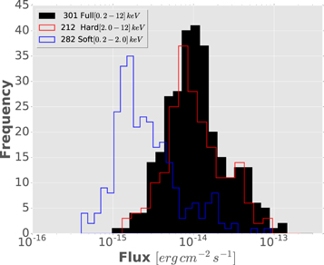
Figure 6. Flux distribution for our 301 X-ray point-source catalog in soft [0.2–2 keV] (blue histogram), hard [2–12 keV] (red histogram), and full [0.2–12 keV] (black-filled histogram) bands.
Download figure:
Standard image High-resolution imageConsidering the level of background and the same spectral assumptions of both surveys, we conclude that our results are comparable with those of Ranalli et al. (2013) for the XMM-Newton survey in the Chandra Deep Field South that presents a similar sky area of  (equivalent to 28
 8 × 288) but twice nominal exposure time of 3.45 Ms. In fact, they achieved an X-ray sensitivity of 6.6 × 10⁻¹⁶ erg cm−2 s−1, in the 2–10 keV band, which is roughly twice as sensitive as our survey.
4.2. Sky Coverage and Log N(>S)–Log S Analysis
4.2.1. Sky Coverage
To estimate the expected source number distribution for our survey, we proceeded as follows: first, we calculated the sky coverage as a function of the X-ray flux from our sensitivity maps in every observation (PN images) and energy band. The sky coverage is defined as the solid angle within which a source with a certain X-ray flux can be detected with ML ≥ 6. The sensitivity maps were created by the task esensmap during the source detection processes. These maps represent the count rate that a source needs to be detected, in a specific position and energy band. These maps are produced with the same detection threshold adopted in the source detection procedure (ML ≥ 6, see Section 2.2). Each map was divided into circular areas of three pixels radius by considering the XMM-Newton PSF size and the source detection cell of 5 × 5 pixels used during the source detection process (with image binning of 4'' pixel side). We obtained and added the corresponding count rate and solid angle of every circular region, to obtain the cumulative survey area as a function of the mean flux limit.
We note that the total sky coverage of the survey is reduced to 295 × 295 equivalent to 0.241 deg2 due to the masking applied (see Figure 1 in Section 2.3). In Figure 7, we present the sky-coverage fluxes of our survey, computed from our sensitivity maps with the lowest fluxes at 2.7 × 10⁻¹⁶ erg s−1 cm−2, 1 × 10⁻¹⁵ erg s−1 cm−2, and 7.3 × 10⁻¹⁶ erg s−1 cm−2 in the soft, hard and full band, respectively. The faintest sources detected in our catalog are consistent with these fluxes.
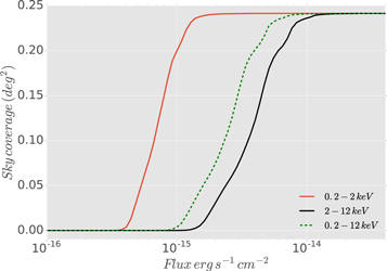
Figure 7. Sky coverage curves as a function of flux in the hard (black line), soft (red line), and full (green-dotted line) X-ray bands computed from the combination of the individual sensitivity maps of each observation.
Download figure:
Standard image High-resolution image4.2.2. Log N(>S)–Log S
The source counts distribution (Log N(>S)–Log S) was obtained using our source catalog and the sky-coverage curves that were computed previously. The Log N(>S)–Log S represents the observed source counts N(>S) as a function of the flux limits S of our survey, recovered from the sensitivity maps. We showed the form of the Log N(>S)–Log S distributions using the integral source counts form N(>S) as the number of sources per unit of sky area with measured flux higher than S:

where Ωi
is the sky coverage (in deg2) of the source i in the bin, Sj
is the flux of the faintest element in the bin; the sum goes for the whole source list considering sources with flux Si
> Sj
. Based on Poissonian statistics, the error bars are defined as  with k as the total number of sources with Si
> Sj
.
with k as the total number of sources with Si
> Sj
.
Nineteen out of our 301 sources were detected in only one of the 13 observations, probably due to intrinsic variability. If they were detected during X-ray luminosity bursts, then their fluxes would not be representative of their average luminosity and could therefore bias the source counts distribution of our survey toward artificially high fluxes. Hence, we decided not to include these sources in our (Log N–Log S) analysis, and we used only 282 X-ray objects that have been detected in at least two observations (see Table 3).
Table 3. Summary of  Distribution for Soft, Hard, and Full-band Bands, Respectively
| Flux a | N( > S) b | Nc | N( > S) b | Nc | N( > S) b | Nc |
|---|---|---|---|---|---|---|
| (S) | Soft | Hard | Full-band | |||
| 3.71 × 10⁻¹⁶ | 1107 ± 67 | 269 | ⋯ | ⋯ | ⋯ | ⋯ |
| 6.75 × 10⁻¹⁶ | 1015 ± 63 | 260 | ⋯ | ⋯ | ⋯ | ⋯ |
| 1.23E × 10−15 | 845 ± 57 | 220 | 1753 ± 123 | 205 | ⋯ | ⋯ |
| 2.23 × 10⁻¹⁵ | 568 ± 49 | 132 | 1313 ± 94 | 197 | 802 ± 58 | 196 |
| 4.05 × 10⁻¹⁵ | 284 ± 34 | 68 | 852 ± 63 | 181 | 745 ± 54 | 187 |
| 7.36 × 10⁻¹⁵ | 140 ± 24 | 35 | 562 ± 49 | 130 | 626 ± 50 | 156 |
| 1.34 × 10⁻¹⁴ | 85 ± 19 | 21 | 280 ± 34 | 67 | 367 ± 38 | 91 |
| 2.43 × 10⁻¹⁴ | 21 ± 9 | 5 | 152 ± 25 | 36 | 185 ± 27 | 46 |
| 6.04 × 10⁻¹⁴ | 4 ± 4 | 1 | 24 ± 10 | 6 | 48 ± 15 | 10 |
| 1.10 × 10⁻¹³ | ⋯ | ⋯ | 4 ± 3 | 1 | 9 ± 5 | 3 |
Notes.
a Flux limits in erg s−1 cm−2. b Source counts per deg2 by band with Poissonian error. c Cumulative number of filtered sources (as described in the text) observed with fluxes corrected for galactic absorption higher than the flux limits.Download table as: ASCIITypeset image
In Figure 8, we present our Log N(>S)–Log S distribution for the hard and soft bands. We compared our source counts cumulative distribution with previous XMM-Newton and Chandra surveys, such as: Luo et al. (2017) with the 7 Ms Chandra deep field-south survey with a small coverage (0.13 deg2) and Civano et al. (2016) with the 4.6 Ms COSMOS-Legacy survey (2.2 deg2) (Chandra). Then, we compared with Carrera et al. (2007) and Chen et al. (2018) (XMM-Newton) for medium areas of 4.8 and 5.3 deg2, respectively. Additionally, for the hard band we compared with the 3.45 Ms XMM-Newton deep survey in the CDF-S (Ranalli et al. 2013) with a sky coverage of 288 × 288, comparable with our field of 295 × 295.
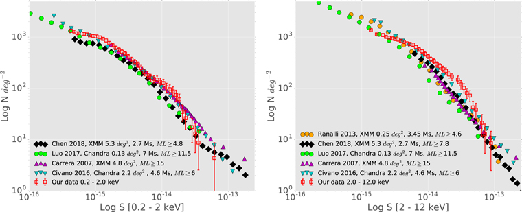
Figure 8. Comparison of our  distribution (red squares) for the 269 filtered sources observed in the soft band (left-hand panel) and 205 sources observed in the hard band (right-hand panel) with previous representative surveys at small ( ≤ 1 deg2) and medium sky coverages ( ≤ 5.5 deg2).
Download figure:
Standard image High-resolution imageOur Log N(>S)–Log S distributions are in good agreement with the results of the aforementioned works, except for the hard X-ray "bump" at (1–4) × 10−14 erg cm−2 s−1, which was also seen by Puccetti et al. (2009). This deviation might be due to low counting statistics induced by our small sky-coverage survey (cosmic variance) plus the effects of the difference in the cross-calibration for each survey and the spectral model used for the flux estimation. A summary of our source counts cumulative distribution is presented in Table 3 for the soft, hard, and full bands.
4.3. Hardness Ratio and Obscured Sources
The hardness ratio (HR) is a powerful indicator of the intrinsic spectrum of an X-ray source. The HR value can also indicate the amount of obscuration by assuming a simple power-law model. The HR is defined as follows:

where S are the soft band count rates (0.2–2 keV) and H are the hard band count rates (2–12 keV).
The source count rates used in our analysis are supplied by edeteck_stack through the task emldetect. We considered the total counts from the PN camera in the 13 observations and the total cleaned exposure time corrected for vignetting. In our analysis, we used a threshold limit of HR ≥ −0.2 to distinguish between unobscured sources or type 1 (Gilli et al. 2007) and obscured sources or type 2 (Szokoly et al. 2004; Marchesi et al. 2016). This threshold is also used in previous works, such as Brusa et al. (2010), who used multiwavelength observations on the XMM-Newton survey of the COSMOS field.
In Figure 9, we present the HR distribution of our sample by using the mentioned HR threshold. We found that 30% (90) of our sources are obscured, whereas 70% (211) are unobscured. The mean HR of our sample is HR = −0.31 ± 0.41.
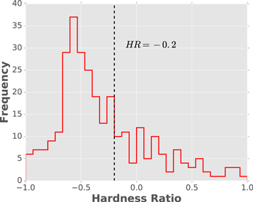
Figure 9. HR distribution of our 301 sources, the black-dashed line at HR = − 0.2 separate between obscured (90) and unobscured sources (211).
Download figure:
Standard image High-resolution imageFigure 10 shows the HR versus z distribution of our catalog. Following Elvis et al. (2012), we included seven curves for different levels of obscuration (log NH = 24, 23.7, 23, 22.7, 22.4, 22, 21), assuming a constant spectral index of Γ = 1.7 and adopting the PN response (QRF) corresponding to the cycle when these observations were taken. We observed that 62 out of 211 sources (29.4%) present obscuration with log NH > 22.
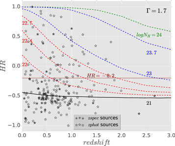
Figure 10. Hardness ratio vs. redshift distribution of 211 sources, dotted lines mark different obscuration levels with  , and 21, calculated assuming a spectral index of Γ = 1.7.
Download figure:
Standard image High-resolution image5. X-Ray and Optical/Infrared Results
We calculated the X-ray luminosities (Lx) of our catalog from the observed flux at soft (0.2–2), hard (2–12), and full (0.2–12) X-ray bands, assuming a Γ = 1.7 power-law spectrum corrected for Galactic absorption (see Section 4). Moreover, following Xue et al. (2011) and Trouille et al. (2011), we applied a K-correction with the equation:

where kcorrection = (1 + z)Γ–2, DL is the luminosity distance and Fx is our X-ray flux. As noted earlier in Section 4.1, we did not apply any further correction for intrinsic absorption in the luminosities reported here.
5.1. Source Type and AGN Identification
We identified a subsample of AGN candidates from our X-ray catalog using the criteria presented by Luo et al. (2017), updated from Xue et al. (2011), and used by Chen et al. (2018) in the XMM-SERVS survey. These three criteria are based on X-ray luminosity, optical/X-ray, and near-IR/X-ray flux ratios. When an X-ray source satisfies at least one of them, we classify it as an AGN candidate.
- 1.An X-ray luminosity threshold Lx > 3 × 1042 erg s−1.
- 2.An X-ray to optical flux ratio threshold of
 .
. - 3.An X-ray to near-IR flux ratio threshold of.
According to the first criterion, we found 173 X-ray sources with L0.2−12 keV > 3 × 1042 erg s−1. For the second criterion, we found 147 objects with  . Finally, for the third criterion we found a total of 117 sources with
  . To represent these results, in Figure 11 we show the F0.2−12 keV versus Fr-band distribution for 185 X-ray sources with magnitude r < 24.8 (left-hand panel) and the F0.2−12 keV versus Fks distribution for 154 sources of our catalog with infrared counterparts (right-hand panel). In both plots, the dark-gray area represents the "typical AGN selection region," while the red diamonds represent sources with L0.2−12 keV ≥ 3 × 1042 erg s−1 and blue circles are those with L0.2−12 keV < 3 × 1042 erg s−1. Finally, by combining the three criteria we found that 204 (∼84%) of 244 sources are AGNs, of which 50% satisfy at least two criteria, and 42% satisfy all three criteria. A redshift estimate is available for 184 out of the 204 AGNs identified here.
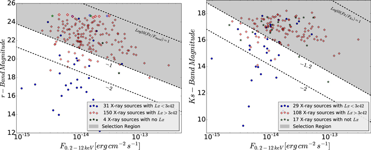
Figure 11. Left-hand panel: F0.2−12 keV vs. r-band distribution for 185 sources from our X-ray catalog with optical counterparts. Filled (173) and unfilled symbols (12) mark those objects with magnitude  and
and  (upper limit), respectively. The black-dotted lines represent the
  flux ratios at −2, −1, and 1, respectively, and the dark-gray area marks the "typical AGN selection region" with
  . Red diamonds, blue circles and green stars mark X-ray sources with L0.2−12 keV < 3 × 1042 erg s−1, L0.2−12 keV ≥ 3 × 1042 erg s−1, and not estimation of L0.2−12 keV, respectively. Right-hand panel: F0.2−12 keV vs. Ks-band distribution for 154 X-ray sources with IR counterparts of our catalog, with the same symbols used in the left-hand figure.
Download figure:
Standard image High-resolution imageFor a comparison, we downloaded Chen et al.'s (2018) catalog (hereafter Chen), which was obtained with the XMM-SERVS survey from their webpage.
17
They used a catalog composed by observations of several instruments, such as: HSC-SSP  , CFHTLS
  , and SDSS
  . To compare our results with Chen, we used three flux ranges 10−15–10−13 erg cm−2 s−1, 10−15–10−14 erg cm−2 s−1 and 10−14–10−13 erg cm−2 s−1, then we count the number of sources with
  in both catalogs (considering the error propagation; see Table 4). Overall, our results are consistent with Chen; that is, in the first range we found
  of our sources with
  , while Chen had
  . Meanwhile, for fainter sources (10−15–10−14 erg cm−2 s−1) we detected discrepancies, mainly due to the magnitude limit used by Chen of
  with HSC, while we reached
  for upper limit detection with GTC.
Table 4. Comparison Table of Fx/Fr AGN Criterion of Chen et al. (2018) and Our Results
| Flux Range | Chen Catalog | Chen Catalog | XMM175UNDF | XMM175UNDF | |
|---|---|---|---|---|---|
| (erg cm−2 s−1) | error ( + σ, − σ) |

| error ( + σ, − σ) | ||
| 10−15–10−13 | Sources | 4887 | ⋯ | 180 | ⋯ |
| AGNs | 4057 | 4257, 3805 | 143 | 148, 133 | |
| AGNs/Sources | 0.83 | 0.871, 0.779 | 0.8 | 0.822, 0.739 | |
| 10−15–10−14 | Sources | 2770 | ⋯ | 82 | ⋯ |
| AGNs | 2248 | 2398, 2061 | 58 | 61, 50 | |
| AGNs/Sources | 0.812 | 0.866, 0.744 | 0.7 | 0.744, 0.61 | |
| 10−14–10−13 | Sources | 2117 | ⋯ | 98 | ⋯ |
| AGNs | 1809 | 1859, 1744 | 86 | 87, 83 | |
| AGNs/Sources | 0.855 | 0.878, 0.824 | 0.878 | 0.888, 0.847 | |
Download table as: ASCIITypeset image
In Figure 12, we present the redshift versus  distribution of our X-ray catalog, with spec-z sources (cross symbols, up to z ∼ 2.7) and photo-z sources (circles/stars symbols). We classified our targets into three broad luminosity groups: Low-Luminosity AGNs, with Lx < 1042 erg s−1, Seyferts, with Lx = 1042–1044 erg s−1, and Quasars, with Lx > 1044 erg s−1. In our sample, we count 139 Seyfert galaxies, 41 Quasars, and 4 LLAGNs (see Table 5).
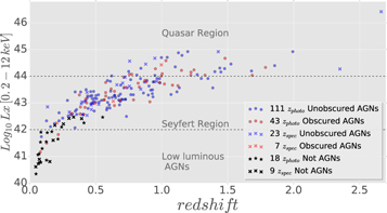
Figure 12. Redshift vs. ![${\mathrm{Log}}_{10}\,{Lx}\,[0.2\mbox{--}12\,\mathrm{keV}]$](https://content.cld.iop.org/journals/0004-637X/919/1/18/revision1/apjac0d5dieqn35.gif) distribution for 211 sources of our X-ray catalog. Red and blue symbols represent obscured (50) and unobscured AGNs (134), respectively, where circles/stars are for measurements with zphoto and crosses mark zspec, respectively. Moreover, we subclassified the sources as a function of their luminosity as Quasars Lx > 1044, Seyfert Lx = 1042–1044, and LLAGNs Lx < 1042 erg s−1. The black symbols represent 27 No-AGNs X-ray candidates.
distribution for 211 sources of our X-ray catalog. Red and blue symbols represent obscured (50) and unobscured AGNs (134), respectively, where circles/stars are for measurements with zphoto and crosses mark zspec, respectively. Moreover, we subclassified the sources as a function of their luminosity as Quasars Lx > 1044, Seyfert Lx = 1042–1044, and LLAGNs Lx < 1042 erg s−1. The black symbols represent 27 No-AGNs X-ray candidates.
Download figure:
Standard image High-resolution imageTable 5. AGNs Classification Resume for the Whole XMM175UNDF Catalog
| Counterparts | Type | Number |
|---|---|---|
| with redshift (211) | Quasar | 41 |
| Seyfert | 139 | |
| LLAGN | 4 | |
| No-AGNs selected a | 27 | |
| No redshift (34) | Unclassified-AGN b | 20 |
| No-AGNs selected a | 14 | |
| No Counterpart (57) | Unknown c | 57 |
| Total | 301 | |
| AGNs | Criterion 1 | 173 |
| Criterion 2 | 147 | |
| Criterion 3 | 117 | |
Notes. The Quasar, Seyfert and LLAGN type is selected as defined in the text.
a Sources which did not satisfy any AGN criterion. b AGNs with no redshift estimation. c Sources without optical counterpart.Download table as: ASCIITypeset image
In Figure 13, we show the distribution of the absolute  magnitude
  versus L0.2−12 keV of 131 source of our catalog with
  , we can observe a clear separation between AGNs (red and blue symbols) and non-active sources (dark symbols). Additionally, we distinguish Seyfert galaxies and optical QSOs by using the equation
  (Schmidt & Green 1983; Schneider 2006).
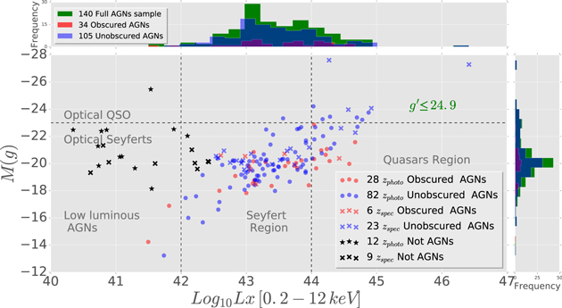
Figure 13. X-ray luminosity L0.2−12 keV vs. Absolute  band magnitude distribution of 160 X-ray sources with
  . Blue and red symbols represent unobscured (105) and obscured (34) AGNs, respectively, where circles/stars are for measurements with zphoto and crosses mark zspec, respectively. Black symbols represent No-AGN candidates (21). The green, blue, and red histograms show the dispersion of the full, unobscured, and obscured AGN samples in function of Lx and M(g). The horizontal and vertical lines divide the chart in different regimes, the optical and X-ray transition between Seyferts, Quasars and/or QSOs.
Download figure:
Standard image High-resolution image6. Discussion
Following the analysis presented in the previous section, we selected a list of X-ray emitting AGNs. From a subsample of 244 (81%) X-ray sources with optical/IR counterparts (301 detected in the XMM175UND-Field, see Appendix C, Table 6), we found a total of 204 AGNs, where 50% of them satisfied at least two of the three criteria outlined in Section 5.1. This fraction increases to 90% (219 AGNs) if we suppress the magnitude limit  in the Fx/Fr criterion. This result is consistent with Chen et al. (2018) (by taking into account our differences in magnitude limits).
Possible causes for the lack of counterpart associations for the remaining (19%) of our X-ray sources are: (1) the magnitude limit  in our GTC catalog, (2) the sensitivity of the WISE cameras, and (3) possible spurious sources that are not yet removed from the catalog.
The absence of high-z sources is likely to be due to the limited redshift of the bulk of our training set (99% up to z ∼ 1.5). Therefore, to explore the possible high-z contents of our survey, it is necessary to proceed with a spectroscopic survey around the remaining 33 X-ray sources with Optical/IR counterparts without z estimations. Finally, the AGN criteria selection that we used are highly reliable for luminous sources, but in some cases at low Lx ( ∼ 1042 erg s−1) we could be misclassifying starburst galaxies as AGN candidates. Nevertheless, these results are in agreement with the lack of bright Quasar and the spatial distribution of Seyfert galaxies population below z ≃ 1 (Fiore et al. 2003; Pâris et al. 2018).
As a comparison, Marchesi et al. (2016) report a catalog of 4016 X-ray sources with a sky-coverage survey that is nine times larger than ours (2.2 deg2) in the 4.6 Ms Chandra COSMOS-Legacy Survey. They found a total of 1582, 717, 17, and ∼11 sources at redshift ranges z = 1–2, 2–3, 4–5, and z > 5, respectively. These observations are the combination of two surveys, the 1.8 Ms C-COSMOS survey (Elvis et al. 2009) and a 2.8 Ms Chandra observations (Civano et al. 2016). Their sensitivities of 1.9 × 10⁻¹⁶, 7.3 × 10⁻¹⁶ and 5.7 × 10⁻¹⁶ erg s−1 cm−2 in the soft, hard, and full bands, respectively, were obtained in a region of 0.5 deg2 (two times wider and deeper than our survey) and 1.8 Ms (equivalent to our exposure). Considering these results, and based on the assumption that the 11 sources at z > 5 are the faintest ones observed in the region with the highest sensitivity (0.5 deg2) distributed homogeneously, we could expect ∼4 sources at z > 5 in our survey by rescaling our sky coverage (0.241 deg2), exposure time (1.75 Ms) and sensitivities with Marchesi et al. (2016).
Meanwhile, Ranalli et al. (2013) with the 3.45 Ms XMM-Newton survey in the Chandra Deep Field South (similar sky coverage 0.231 deg2, twice nominal exposure time, and two times deeper in the hard band), reports a catalog of 339 sources at hard band with sensitivities of 6.6 × 10⁻¹⁶ erg cm−2 s−1 and 137 in super hard band [5–10 keV] using a significance of ML > 4.6 (lower than our ML > 6). Since we found 212 hard and 82 super hard sources, these results are consistent with Ranalli et al. (2013), considering lower exposure and higher ML.
A comparison of our source counts cumulative distribution with previous results showed an overall good agreement for different type of XMM-Newton and Chandra surveys in small and medium sky area coverage. Even so, there are small discrepancies in the  in the hard X-ray band. These differences can be explained by the effect of low counting statistics (cosmic variance), due to the small sky coverage of our survey, plus possible effects of the difference in the cross-calibration and the spectral model used for each survey.
7. Summary and Conclusions
In this paper, we present a deep XMM-Newton survey of the XMM175UND-Field, which consists of 13 observations centered on the same field of  obtaining a total exposure time of 1.75 Ms (with cleaned PN of 1.372 Ms). An optical follow-up with the GTC telescope and a cross-correlation analysis in optical and infrared bands allowed us to perform a multi-band study of our X-ray catalog. A summary of our results is given below:
- 1.We computed the X-ray source detection using the new task edetect_stack with the standard XMM-Newton bands (0.2–0.5, 0.5–1, 1–2, 2–4.5, 4.5–12 keV) and significance threshold of p ≃ 2.5 × 10⁻³ (equivalent to ∼3σ). We obtained a reliable catalog of 301 X-ray point-like sources with flux limits of 4.03 × 10⁻¹⁶, 1.3 × 10⁻¹⁵ and 9.8 × 10⁻¹⁶ erg s−1 cm−2 for the soft, hard, and full band, respectively. Additionally, we did a detailed comparison analysis with the 4XMM catalogs of Webb et al. (2020) and Traulsen et al. (2020), resulting in a respective consistency of 96% and 94% with both catalogs.
- 2.We used the LR technique to perform a cross-correlation analysis of our X-ray catalog with an optical catalog of 43,068 objects produced by the OSIRIS instrument at GTC and an infrared-WISE public repository. We were able to detect optical/IR counterparts for 81% (244) of the whole XMM175UNDF catalog.
- 3.We computed our own photometric redshifts by using PhotoRApToR with a training set of 824 sources detected in our field (33 from our own GTC observations). About 99% of our spec-z catalog are contained in the range zspec = 0–1.5, thus we constrained our photo-z reliability up to z = 1.5. Then, we achieved a ∼93% of redshift completeness for our 227 X-ray sources with optical counterparts.
- 4.We calculated the distribution using the sky coverage of our survey in a region of 0.241 deg2. We found a general good agreement with previous XMM-Newton and Chandra surveys in small and medium areas.
- 5.We obtained the HR distribution of our source list and assuming a threshold of HR ≥ − 0.2, we found that 30% (90) of the sources are obscured, of which 87.9% have. We obtained a mean and error HR for the full catalog of HR = − 0.31 ± 0.41.
- 6.We used the criteria by Luo et al. (2017) to select AGN candidates of our X-ray catalog based on their optical/IR and X-ray properties. We classified 204 objects as AGNs; of which 139 are Seyfert galaxies, 41 luminous Quasar, 4 LLAGNs, and 20 unclassified AGNs.


Y.K. acknowledges support from grant DGAPA-PAPIIT 106518 and from program DGAPA-PASP, and also acknowledges for the CONACyT Project: A1-S-22784. A.L.L. and M.E.C. acknowledge support from CONACyT grant CB-2016-286316. We also thank CONACyT for the grant to course my PhD and the research grants CB-A1-S-25070 (YDM), and CB-A1-S-22784 (DRG).
Facilities: XMM-Newton - , GTC(OSIRIS). -
Software: The entire X-ray dataset that we used in this article are available in the public XMM-Newton repositories, the "XMM-Newton Science Archive" on http://nxsa.esac.esa.int/nxsa-web/#home. The source code used for the cross-correlation analysis Xcorr is available at http://saada.u-strasbg.fr/docs/fxp/plugin/ (Pineau et al. 2011). Meanwhile, PhotoRApToR is available at http://dame.oacn.inaf.it/dame_photoz.html (Cavuoti et al. 2015) and the code used for our optical spectral reduction gtcmos version 1.4 is available at https://www.inaoep.mx/ydm/gtcmos/gtcmos.html (Gómez-González et al. 2016).
Appendix
In this appendix we will present a more detailed explanation of some of the important steps that we made during the preparation of this project, the idea is to simplify the understanding of: (1) the reliability of our results by presenting a deep comparison analysis of our X-ray catalog versus the newest XMM-Newton Survey Science Centre catalogs; and (2) give a precise description of the optical spectral analysis performed with optical sources detected in our own GTC observations over the XMM175UND-Field, which were used in the training set to estimate our photometric redshifts.
Appendix A: 4XMM Catalogs Comparison
The source detection analysis on the XMM175UND-Field in Section 2 led to a preliminary source list of 483 X-ray sources and a final catalog of 301 objects.
During the completion of this work, two papers were published containing X-ray analyses of this same field: the newly obtained 4XMM-DR9 X-ray catalog for individual observations of Webb et al. (2020) (hereafter DR9) and the 4XMM-DR9s catalog for overlapping observations of Traulsen et al. (2020) (hereafter DR9s). Both catalogs were produced by XMM-Newton Survey Science Centre with ML ≥ 6. First, Webb et al. (2020) analyzed 14,041 individual observations from 2000 to 2019 February, finding 550,124 sources in an area coverage of 1152 deg2. Meanwhile, Traulsen et al. (2020) was constructed using the same algorithm edetect_stack employed in this work (see Section 2), they analyzed 1329 stacks with 6604 overlapping observations from 2000 February to 2018 November, finding 288,191 sources in an area of 300 deg2. Both catalogs contain the same 13 pointings that we used in our analysis, with the addition of 10 extra PN small-window calibration observations (each of ∼30 ks) pointed on the blazar 1ES 1553+113 that our survey does not include.
We present here a detailed comparison of our results with these two surveys. By using a cross-correlation radius of 10'' (similar to Chen et al. 2018) based on the positional accuracy, pointing uncertainties and PSF size of XMM-Newton observations; we exhaustively compare: (1) the maximum likelihood distribution of the X-ray sources, (2) the number of elements in each source list, their position and the possible reasons of discrepancy, and (3) the flux distribution of sources in the three surveys.
It is important to mention that the field studied in this paper is very complex thanks to the presence of a very bright source that induces bright spikes at the center of the images. This could easily result in a high number of spurious detections that can fluctuate between two catalogs. Consequently, to have a more reliable comparison between our catalog and the above catalogs, we will not include the sources that lie in the masking region used during our analysis and sources flagged as spurious. As a result of this choice, our survey contains less sources (301) compared to both 4XMM catalogs but with a very similar number of detections in our preliminary source list: 483 objects (see Section 2.3), compared with 477 (DR9s) and 478 (DR9).
In Figure 14, we compared the detection significance for our source list and DR9s. At ML > 6, we observe the same behavior for both samples, while at lower significance (ML < 6) the amount of possible spurious sources increase, which could modify the distribution observed in both catalogs. 18
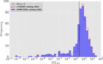
Figure 14. Comparison of the detection significance in our preliminary source list with 483 sources (red) vs. DR9s 566 objects (blue) of which 89 are flagged as spurious. We used the XMM-Newton EPIC/pn maximum likelihood distribution for both samples, the black vertical line refers when MLPN = 6.
Download figure:
Standard image High-resolution imageThen, following Chen et al. (2018), we used a circular region of 10'' to cross correlate both 4XMM catalogs with our preliminary source list (483) and final catalog (301). For DR9s (DR9) we found 421 (406) and 288 (284) common X-ray sources with our preliminary source list and final catalog, respectively. In Figure 15, we show the spatial distribution of the non-common sample (22, green circles) along our XMM175UND-Field; the seven sources with highest off-axis angle  are highlighted with red rectangles. These sources are also the ones with the lowest exposure, as expected < 740 ks, (see Figure 16 left-hand panel). These objects could be spurious sources in the borders of the detectors. The blue rectangles show the five highest exposure sources and the lowest off-axis angle
  (see Figure 16 right-hand panel), three of those objects are likely faint sources detected thanks to the combination of the stacking observations. There are likely some spurious objects ( ∼ 4) detected in the wings of the PSF of a bright source. One exception is the source closest to the bright blazar—this is a clear X-ray source, which has optical and IR counterparts. Since this source lied in the region masked out during our source detection process, we did not include it in our final source list.
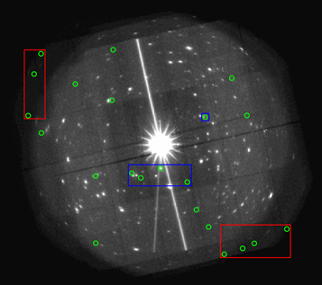
Figure 15. Mosaic image of all observations of the survey at full X-ray band 0.2–12 keV. Green circles mark the 22 non-common sources detected in DR9s but not in our catalog. The red rectangles mark the position of seven objects on the borders of the field, the blue rectangles mark the position of the five closest sources to the center of the field.
Download figure:
Standard image High-resolution image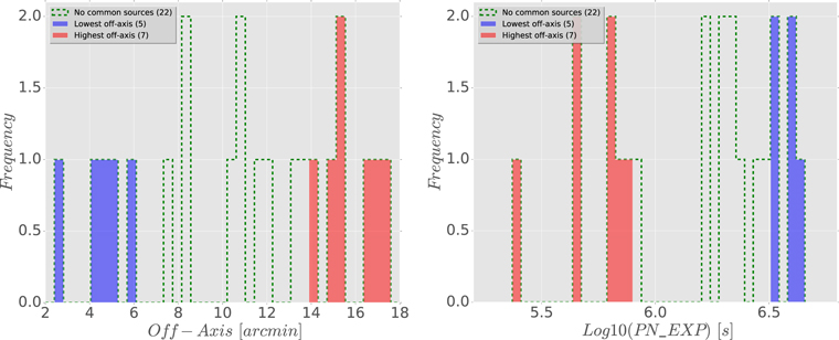
Figure 16. Distribution of 22 sources which are present in DR9s but not in our catalog. Left-hand panel: Off-axis distribution. Right-hand panel: PN exposure distribution. In both figures, the blue and red histograms refer to the lowest ( ) and highest (
 ) off-axis angles.
Download figure:
Standard image High-resolution imageThen, we perform a comparison of the X-ray fluxes obtained by the three catalogs. Figure 17 shows the EPIC-Flux0.2−12 keV distribution of our common sources with DR9s (left-hand panel) and DR9 (right-hand panel). We found a good consistency with both 4XMM catalogs flux estimates (mainly with DR9s); for example, the standard deviations for both distributions are σDR9s = 0.06 and σDR9 = 0.07, respectively. The best linear fit for the common source fluxes are expressed by the equations:
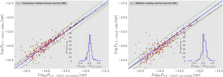
Figure 17. 0.2–12 keV flux distribution for both 4XMM common sources catalogs with our final catalog. Left-hand panel: DR9s vs. our catalog flux distribution for 288 sources. Right-hand panel: DR9 vs. our catalog flux distribution for 284 sources. The blue line marks the  relation, the green-dotted lines refers the σ confidence locus. Right at the bottom, we include the residual distribution for each plot.
Download figure:
Standard image High-resolution imageDue to the intrinsic variability of AGNs, edetect_stack used in this work and by DR9s can reduce the probability to underestimate or overestimate the real fluxes by computing the average flux for the whole overlapping observation for each source. Then, we computed the flux distributions of both 4XMM catalogs. In Figure 18 we can see how DR9 obtains systematically lower fluxes than DR9s, which might be pointing to a real effect of a systematic underestimation of fluxes in DR9. Then, the best linear fits for both 4XMM catalogs are:

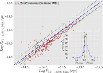
Figure 18. DR9s vs. DR9 0.2–12 keV flux distribution for 278 common sources in both 4XMM and our final catalog. The other elements are similar to Figure 17.
Download figure:
Standard image High-resolution imageAfter this analysis, we can conclude that our results are in satisfactory agreement with both 4XMM catalogs. In summary, in Figure 14 we found a comparable ML distribution for our source list and DR9s. We found only 22 non-common sources with our catalog (most of them are explained above, see Figure 15). Finally, we obtained a solid flux distribution correlation for both 4XMM catalogs (close to 1:1 for DR9s) with σ4XMM−DR9s = 0.06 and σ4XMM−DR9 = 0.07 for DR9s and DR9, respectively (see Figure 17).
Appendix B: GTC Spectral Analysis
Our spectroscopic observations were carried out with the MOS configuration of the instrument OSIRIS with GTC and consists of five observational blocks with 33 slits per block and ∼6–7 stars as fiducial points for astrometry and 1–2 stars for sky spectral subtraction.
Every block was observed in three runs of 15 minutes (45 minutes total exposure), reaching enough sensitivity to allow detection of emission and/or absorption lines in 33 out of ∼100 sources and estimate their spectroscopic redshift. The observations were performed with the R1000R grism, centered at 7430 Å covering the range from 5100 to 10000 Å at a resolution of 2.62 Å pixel−1.
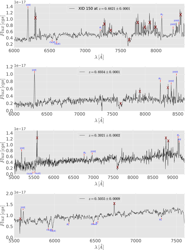
To reduce our spectroscopic data, we used the gtcmos 19 package, as explained in Gómez-González et al. (2016), a semi-automatic pipeline for the reduction of GTC/OSIRIS MOS data, which uses the standard IRAF tasks. In Figure 19, we show an example of four spectra, which present typical signatures of active galaxies (or star-forming processes) such as forbidden emission lines of [O ii], and [O iii] (related to high level of ionization), intense permitted emission lines as Hα, Hβ and some absorption lines, such as CaK, CaH. Out of ∼100 spectra, only four correspond to an X-ray counterpart, but only one of them, XID150 (top panel of Figure 19), presented clear absorption/emission lines leading to a redshift estimate of z = 0.6621. All sources with spectroscopic redshift were included within the training set to compute the photo-z in Section 3.3.
Figure 19. Optical spectra of four of the 33 sources observed with GTC-OSIRIS. All spectra show emissions and/or absorption features, such as Balmer lines, oxygen forbidden lines and calcium-II doublet at the observed wavelengths. The top-most panel shows the spectrum for the XID150 X-ray source at z = 0.6621. Residual sky lines are marked by X sign.
Download figure:
Standard image High-resolution image
Appendix C: Tables
Table 6. Main Parameters of Our Catalog Used Along Our X-Ray to Optical/IR Analysis
| IDX a | R.A. b | Decl. c | ML d | Fxe | HR f | zg | zphoth | Lxi | AngDis_opj |
 k
k
|
 l
l
|
 m
m
| W1 n | W2 o | Frp | FWKsq |
 r
r
|
 s
s
|
|---|---|---|---|---|---|---|---|---|---|---|---|---|---|---|---|---|---|---|
| 1 | 238.9119 | 11.11235 | 104284.8 | 3.04E-13 | −0.5 | 2.6636 | 0.4 | 2.61E+46 | 1 | 19.42 | 19.31 | 19.27 | 15.97 | 15.23 | 4.99E-13 | 1.63E-13 | −0.214 | 0.271 |
| 2 | 238.8756 | 11.36975 | 65311.24 | 1.44E-13 | −0.685 | 0.1343 | 0.15 | 7.14E+42 | 0.85 | 18.79 | 17.97 | 17.45 | 14.91 | 14.66 | 1.73E-12 | 4.30E-13 | −1.079 | −0.476 |
| 3 | 238.7203 | 11.09557 | 39007.43 | 1.18E-13 | −0.51 | 0.756873 | 0.9 | 3.67E+44 | 0.55 | 19.39 | 19.54 | 19.37 | 14.73 | 13.49 | 4.04E-13 | 5.04E-13 | −0.534 | −0.631 |
| 4 | 238.8523 | 11.15929 | 34690.83 | 8.55E-14 | −0.654 | −99 | 1.13 | 7.53E+44 | 0.6 | 20.67 | 20.43 | 20.38 | 16.2 | 15.23 | 1.79E-13 | 1.33E-13 | −0.32 | −0.19 |
| 5 | 239.0276 | 11.27217 | 27177.42 | 8.41E-14 | −0.335 | 0.9481 | 0.58 | 4.70E+44 | 0.72 | 21.68 | 21.26 | 20.88 | −99 | −99 | 8.30E-14 | −99 | 0.006 | −99 |
| 6 | 239.1048 | 11.16245 | 22552.52 | 6.42E-14 | −0.609 | −99 | 1.15 | 6.01E+44 | 0.71 | 21.26 | 20.91 | 20.66 | 16.92 | 15.73 | 1.15E-13 | 6.88E-14 | −0.252 | −0.031 |
| 7 | 239.0026 | 11.06852 | 22232.23 | 7.08E-14 | −0.446 | −99 | 1.04 | 5.07E+44 | 0.91 | 21.51 | 21.32 | 21.12 | 15.95 | 15 | 7.88E-14 | 1.66E-13 | −0.047 | −0.369 |
| 8 | 238.9871 | 11.29352 | 21306.9 | 5.50E-14 | −0.498 | −99 | 0.62 | 1.03E+44 | 0.53 | 22.45 | 22.23 | 21.51 | 17.66 | 16.82 | 3.40E-14 | 3.50E-14 | 0.208 | 0.196 |
| 9 | 238.9754 | 10.99547 | 18809.03 | 7.78E-14 | −0.598 | −99 | 1 | 4.98E+44 | 0.36 | 20.7 | 20.51 | 20.37 | 15.86 | 15.72 | 1.66E-13 | 1.81E-13 | −0.328 | −0.366 |
| 10 | 238.9107 | 11.34319 | 15904.15 | 6.18E-14 | −0.533 | 0.8788 | 0.79 | 2.84E+44 | 0.73 | 21.15 | 20.92 | 20.49 | 15.92 | 15.34 | 1.14E-13 | 1.70E-13 | −0.265 | −0.44 |
| ⋯ | ⋯ | ⋯ | ⋯ | ⋯ | ⋯ | ⋯ | ⋯ | ⋯ | ⋯ | ⋯ | ⋯ | ⋯ | ⋯ | ⋯ | ⋯ | ⋯ | ⋯ | ⋯ |
Notes. The whole table is available online in ASCII format along with this paper.
a ID X-ray name for each source. b R.A. from the X-ray catalog. c Decl. from the X-ray catalog. d Maximum Likelihood significance. e Full-band X-ray flux in units of erg cm−2 s−1. f Hardness Ratio. g Spectroscopic redshift. h Photometric redshift. i Full-band X-ray luminosity in units of erg s−1. j Optical counterpart angular distant in units of arcsec. k optical g-band magnitude. l optical r-band magnitude. m optical i-band magnitude. n Infrared W1-band magnitude. o Infrared W2-band magnitude. p Optical flux at r-band in units of erg cm−2 s−1. q Optical flux at Ks-band in units of erg cm−2 s−1, expressed by the equation Ks = 0.99 × W11 + 0.23. r Ratio between the X-ray and optical at r-band fluxes in log10 scales. s Ratio between the X-ray and infrared at Ks-band fluxes in log10 scales.Only a portion of this table is shown here to demonstrate its form and content. A machine-readable version of the full table is available.
Download table as: DataTypeset image
Footnotes
- 9
The present XMM-Newton catalog with its optical (GTC) and Infrared (WISE/2MASS) counterpart associations is publicly available for further analysis in ASCII format along with this paper. Additionally, the catalog will be uploaded to Vizier.
- 10
- 11
- 12
- 13
Optical System for Imaging and low-Intermediate-Resolution Integrated Spectroscopy (OSIRIS; http://www.gtc.iac.es/instruments/osiris/) is an imager and spectrograph for the optical wavelength range, located in the Nasmyth-B focus of GTC.
- 14
- 15
- 16
- 17
- 18
Sources with ML higher or equal to 6 in the final stacking or at least in one observation in any band are select as an X-ray source; that is, there are X-ray sources selected which have ML < 6 in the final stacking, but with a likelihood ≥6 in at least one band in one or two individual observations (standard selection technique of edetect_stack see Traulsen et al. 2019, for more details).
- 19