


Abstract
HH 211 is a highly collimated jet with a chain of knots and a wiggle structure on both sides of a young Class 0 protostar. We used two epochs of Atacama Large Millimeter/submillimeter Array (ALMA) data to study its inner jet in the CO(J = 3–2), SiO(J = 8–7), and SO(NJ = 89–78) lines at ∼25 au resolution. With these ALMA and previous 2008 Submillimeter Array data, the proper motion of 8 knots within ∼250 au of the central source is found to be ∼0068 per year (∼102 km s−1), consistent with previous measurements in the outer jet. At about four times higher resolution, the reflection-symmetric wiggle can be still fitted by a previously proposed orbiting jet source model. Previously detected continuous structures in the inner jet are now resolved, containing at least 5 subknots. These subknots are interpreted in terms of a variation in the ejection velocity of the jet with a period of ∼4.5 yr, shorter than that of the outer knots. In addition, backward and forward shocks are resolved in a fully formed knot, BK3, and signatures of internal working surface and sideways ejection are identified in position–velocity diagrams. In this knot, low-density SO and CO layers are surrounded by a high-density SiO layer.
Export citation and abstract BibTeX RIS
1. Introduction
Protostellar jets play an important role in the star formation process. In the theoretical picture, they are believed to be launched and to remove excess angular momentum from the inner part of the accretion disk within 1 au of protostars (Frank et al. 2014; Lee 2020). Two competing models of jet launching are proposed: the disk-wind model (Konigl & Pudritz 2000) and the X-wind model (Shu et al. 2000). Both models predict a fast-dense collimated jet propagating along the rotation axis of the system. As the inner parts of the disks where the jets are launched are on scales (≤1 au) that are not easy to resolved with current instruments, we use the jet properties (e.g., jet morphology and rotation) and knot (shock) structures observed on large scales to constrain the accretion processes and physical conditions during the early phase of star formation. The goal is to study the mechanism that would remove angular momentum near the protostar.
HH 211 is a well-studied jet consisting of a chain of well-defined knots and is highly collimated with a small-scale wiggle (Lee et al. 2010), and thus it is a good candidate for studying the physical properties of the jet and knots. It is located in the IC 348 complex of Perseus at a distance of 321 ± 10 pc (Ortiz-León et al. 2018) and powered by a low-mass (∼0.08 M⊙, after being updated with the new distance from Lee et al. 2019) Class 0 protostar (Froebrich et al. 2003; Froebrich 2005). It has been detected in H2 (McCaughrean et al. 1994) as well as in SiO, SO, and CO (Gueth & Guilloteau 1999; Hirano et al. 2006; Palau et al. 2006; Lee et al. 2007). The jet consists of a large number of knots on both sides of the central source, with an inclination angle of only ∼9° to the plane of sky (Jhan & Lee 2016). Therefore, HH 211 is a suitable source for studying the backward and forward shocks and sideways ejection.
With the Atacama Large Millimeter/submillimeter Array (ALMA), we not only confirm the previously found wiggle structure, proper motion, and knot structures, but also study the morphological relation of the regions seen in the CO(J = 3–2), SiO(J = 8–7), and SO(NJ = 89–78) lines. SiO and SO are shock tracers (Martin-Pintado et al. 1992; Schilke et al. 1997), and CO and SO can both trace jet and outflow. However, their relation is still unclear because the resolution is insufficient to separate them. They may or may not trace material of different densities ejected from different parts of the disk. Now, we have a higher resolution (up to ∼006, which is four times better than in the previous study in Lee et al. 2009) to resolve the jet and its knots in order to address this issue.
2. Observations
Observations toward the HH 211 system were obtained with ALMA in 2015 and 2016. The 2015 observations (cycle 3; Project ID: 2015.1.00024.S) were already reported in Lee et al. (2018). They have the same correlator setup as the 2016 observations (Project ID: 2016.1.00017.S), but a higher angular resolution to search for jet rotation. Here we only summarize the 2016 observations and compare both observations in Table 1.
Table 1. Observation Logs
| Observation | Projected | Angular | Time on | Number of | Sensitivity |
|---|---|---|---|---|---|
| Time (yr) | Baselines (m) | Resolution (SiO) | Target (minutes) | Antennas | (SiO, mJy beam−1) |
| 2015.9 | 15–7930 | 007 × 005 | 123 | 37–41 | 2.2 |
| 2016.8 | 13–3145 | 013 × 008 | 132 | 43 | 1.0 |
Download table as: ASCIITypeset image
HH 211 has been mapped with ALMA at ∼358 GHz in Band 7 with one pointing toward the center. A C40-7 array configuration was used with 43 antennas. Two executions were carried out in 2016 in cycle 4, both on October 10. The projected baselines were 13–3145 m. We had five spectral windows in the correlator setup, four for molecular lines at a velocity resolution of ∼0.212 km s−1, and one for the continuum at a velocity resolution of ∼0.848 km s−1. The CASA package was used to calibrate the data for passband, flux, and gain. The quasars J0238+1636, J0237+2848, and J0336+3218 were used as the flux, bandpass, and gain calibrator, respectively. A phase-only self-calibration derived from the continuum was also applied to the uv data in order to improve the image fidelity and reduce the sidelobes. Because the signal-to-noise ratio of the uv data in long baselines is lower than 3, we only used the continuum data with uv distance <1000 m to derive the solution for the self-calibration and applied the self-calibration to the data with a uv distance <1000 m.
The CASA package was used to image the data. We used CONCAT to combine both the 2015 and 2016 data, and then CLEANed the combined data to generate various line-intensity maps with a velocity resolution of ∼1 km s−1. In order to better show the structure of the jet and outflow shells, we used a robust weighting factor of 2 for the visibility to generate the maps. The resulting CO(J = 3–2), SiO(J = 8–7), and SO(NJ = 89–78) maps have a noise level of ∼1.1, 1.1, and 1.0 mJy beam−1, respectively. The synthesized beam has a size of 0139 × 0083 at a position angle (P.A.) of −98 for SiO, 0129 × 0069 at a P.A. of −89 for CO, and 013 × 0069 at a P.A. of −78 for SO. We also used a robust weighting factor of 0.5 for the visibility to generate higher resolution maps to search for jet rotation and to study shock structures in knot BK3. The resulting CO, SiO, and SO maps have a noise level of ∼1.3, 1.2, and 1.2 mJy beam−1, respectively. The synthesized beam has a size of 0109 × 0059 at a position angle (P.A.) of −122 for SiO, 0095 × 0057 at a P.A. of −137 for CO, and 0095 × 0057 at a P.A. of −130 for SO. In these maps, the velocities are in the LSR system.
3. Results
In HH 211, the systemic velocity is Vsys = 9.2 ± 0.1 km s−1 (Gueth & Guilloteau 1999). In this system, the jet has a position angle of 1161 with the southeastern (SE) component tilted toward us (Gueth & Guilloteau 1999). The continuum emission peak is at the position of α(2000) = 3h43m568054 and δ(2000) = 32°00'50189 (Lee et al. 2018).
3.1. Jet Morphology
SiO(J = 8–7), CO(J = 3–2), and SO(NJ = 89–78) are detected on both sides of the central source, and their emission intensity maps are shown in Figures 1(a)–(c), respectively. As seen before (Lee et al. 2009), the jet in these lines is highly collimated with a small wiggle and consists of a chain of knots, even though the SO emission is relatively weak. Moreover, SiO, SO, and CO emissions trace a bow-shock structure for knot BK3 in the jet (green box in Figure 1).
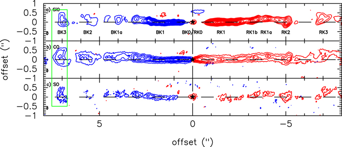
Figure 1. (a) SiO emission map. The blue and red contours are the blueshifted (−24.8 ≤ V ≤ 9.2 km s−1) and redshifted (43.2 ≥ V ≥ 9.2 km s−1) emissions of the SiO. The contour levels start at 3σ with a step of 6σ, and σ is ∼0.2 and 0.19 mJy beam−1 for the blueshifted and redshifted sides, respectively. (b) CO emission map. The blue and red contours are the total high-velocity blueshifted (−14.8 ≤ V ≤ 1.2 km s−1) and the total high-velocity redshifted (35.2 ≥ V ≥ 19.2 km s−1) emissions of the CO, and the contour levels start at 3σ with a step of 6σ, and σ is ∼0.3 mJy beam−1. (c) SO emission map. The blue and red contours are the blueshifted (−19.8 ≤ V ≤ 9.2 km s−1) and redshifted (41.2 ≥ V ≥ 9.2 km s−1) emissions of the SO, and the contour levels start at 3σ with a step of 6σ, and σ is ∼0.21 and 0.19 mJy beam−1, respectively.
Download figure:
Standard image High-resolution imageIn channel maps of these emissions (Figure 2 for SiO, Figure 3 for CO, and Figure 4 for SO), the jet appears increasingly collimated going from low to high velocity. In CO, the jet is seen at high velocity (VLSR ≤ 0.2 km s−1 and VLSR ≥ 18.2 km s−1), and outflow shells are seen at low velocity (0.2 km s−1 ≤ VLSR ≤ 18.2 km s−1), as seen before (Gueth & Guilloteau 1999; Lee et al. 2007). This distribution is also seen in other objects (Santiago-García et al. 2009; Lee et al. 2015). SO traces the jet as SiO and CO does, and shows evidence of shell-like structure at VLSR = 9.2 km s−1 within 2'' of the central source tracing the base of the outflow. All three lines can also trace bow-shock structures, e.g., at velocity ∼−8.8 and 0.2 km s−1 on the blueshifted side.
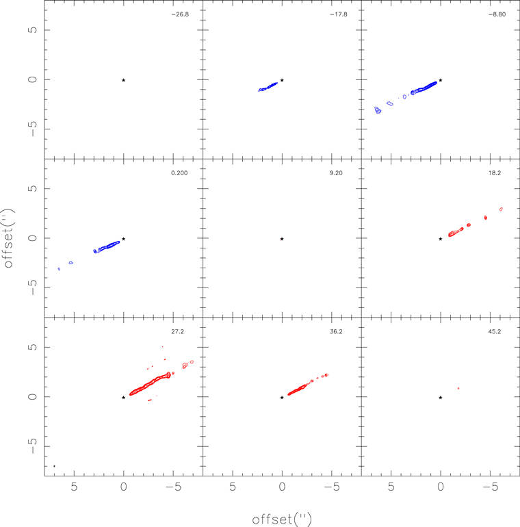
Figure 2. SiO channel maps from −26.8 to 45.2 km s−1 with a step of 9 km s−1 and a velocity resolution of 9 km s−1. The contour levels start at 10σ with a step of 20σ, and σ is ∼0.38 mJy beam−1. The number in the top right corner is the radial velocity of the maps in km s−1.
Download figure:
Standard image High-resolution image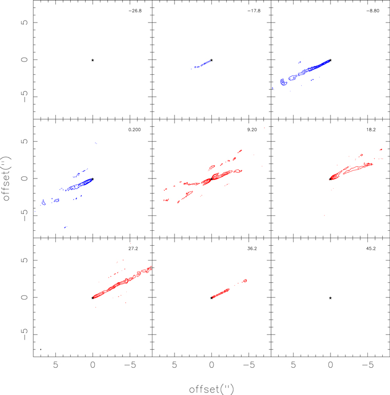
Figure 3. CO channel maps from −26.8 to 45.2 km s−1 with a step of 9 km s−1 and a velocity resolution of 9 km s−1. The contour levels start at 5σ with a step of 10σ, and σ is ∼0.38 mJy beam−1. The number in the top right corner is the radial velocity of the maps in km s−1.
Download figure:
Standard image High-resolution image
Figure 4. SO channel maps from −26.8 to 45.2 km s−1 with a step of 9 km s−1 and a velocity resolution of 9 km s−1. The contour levels start at 5σ with a step of 10σ, and σ is ∼0.37 mJy beam−1. The number in the top right corner is the radial velocity of the maps in km s−1.
Download figure:
Standard image High-resolution image3.2. Proper Motion
In 2008, we observed HH 211 at a resolution of 025 with the Submillimeter Array (SMA; Lee et al. 2009, Figure 5(c)). Therefore, the proper motion can be estimated by measuring the position shift of the knots from the 2008 SMA observation to the 2016 ALMA observation (Figures 5(a) and (b)). The time interval is 7.72 yr. We first degraded the 2016 ALMA map from 008 to 025 resolution and aligned the maps with the continuum peaks. In these two epochs, eight knots within ∼8'' of the central source, four on each side of the source, are used for proper motion measurement. We measured the peak positions of these knots (Figure 5) and calculated the position shift of the knots. The error bar of position shift is assumed to be one-third of the beam size along the jet axis. The proper motion is then estimated to be ∼0068 ± 001 per year. With the new distance of 321 pc, the transverse velocity is ∼102 ± 16 km s−1. Thus, the inclination angle is refined to be ∼11°, using a mean radial velocity of ∼20 km s−1 estimated in Section 3.5.
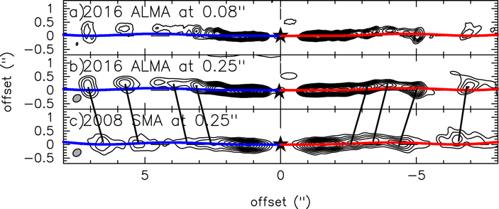
Figure 5. Comparison between the observed jet structure and the orbiting jet source model. The observed jets here are rotated by 261 clockwise. (a) SiO map at 008 resolution of the 2016 ALMA observation before convolution. The contour levels start at 3σ with a step of 6σ, and σ is ∼0.17 mJy beam−1. (b) SiO map at 025 resolution of the 2016 ALMA observation after convolution. The contour levels start at 3σ with a step of 30σ, and σ is ∼1.6 mJy beam−1. (c) SiO map at 025 resolution of the 2008 SMA observation. The contour levels start at 3σ with a step of 3σ, and σ is ∼1.98 mJy beam−1.
Download figure:
Standard image High-resolution imageWe then compared our result with the previous SMA result reported in Jhan & Lee (2016) for the outer parts of the jet at a distance from 5'' to 16''. We first refined the previous SMA measurements by taking out the 2004-epoch data because its resolution is the lowest (∼12) and the UV coverage is the poorest of those in all epochs. The refined proper motion (triangles in Figure 6) is 30% lower than that measured before, but is closer to our current ALMA measurement for the inner jet, as shown in Figure 6. The figure shows that the velocity of the jet is roughly constant at a distance from 1000 to 5000 au (3''–16'') within the error bar, although there could be a slight decrease in velocity with distance, as shown by the linear fit.
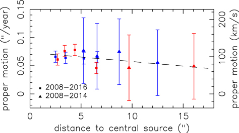
Figure 6. Relation of the proper motion and distance of the knots to the central source. The squares represent the proper motion measurements using 2016 ALMA results and 2008 SMA results. The triangles represent the proper motion measurements using 2008, 2010, and 2013 SMA results, i.e., the measurements of Jhan & Lee (2016) without 2004 SMA results. The measurements of the knots on the redshifted side are plotted in red, and the measurements of the knots on the blueshifted side are shown in blue. The dashed line is a linear fit of proper motion and distance of all knots in both measurements.
Download figure:
Standard image High-resolution image3.3. Wiggle Structure
A reflection-symmetric wiggle has been detected in the jet and was modeled with an orbiting jet source model in Lee et al. (2010). The same model with the same parameters was later used to fit the wiggle in three other epochs (2004, 2010, and 2013) of the SMA data of the SiO line (Jhan & Lee 2016). Now, we can verify whether the model can still fit the same wiggle in our ALMA observation in the inner part of the jet at higher resolution. In our mapped region, the jet shows one to two wiggle cycles, as shown in Figure 5(a). After adjustment for proper motion, the previous best-fit parameters still roughly fit the pattern of the wiggle but with some deviations, especially in the regions, from 3'' to 6'' and from −3'' to −4'' where the peaks of the knots deviate to the north from the model. We discuss the deviations in more detail in Section 4.1.
3.4. Kinematics Perpendicular to the Jet Axis
To study the jet kinematics perpendicular to the jet axis, we present the position–velocity (PV) diagrams along cuts perpendicular to the jet axis in SiO and CO emissions (Figures 7–8) centered at the SiO emission peaks, which have a distance of 05–2'' from the central source. We identified three velocity components in the diagrams, marked by boxes of different colors in the figures: a low-velocity component in red boxes with a wide spatial range, a medium-velocity triangular component in green boxes, and a high-velocity linear component in blue boxes. The low-velocity component is seen mainly in CO, tracing the outflow shell as discussed in Section 3.1. The medium-velocity triangular structure appears in CO and SiO. The high-velocity linear structure is also seen in CO and SiO with almost the same velocity range in these two lines. This high-velocity structure traces the jet itself, as seen in the channel maps. However, the highest velocity of the jet gradually slows down with increasing distances (as can be seen in blue boxes at different distance, or see Figure 8 in Lee & Sahai 2004), and then the high-velocity parts merge with the triangular components in some of the diagrams at large distances.
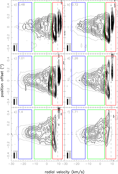
Figure 7. SiO (gray contour) and CO (black contour) PV diagrams of the blueshifted knots along cuts perpendicular to the jet axis. For SiO, the contour levels start at 3σ with a step of 15σ, and σ is ∼0.95 mJy beam−1. For CO, the contour levels start at 3σ with a step of 3σ, and σ is ∼1.1 mJy beam−1. The horizontal dashed lines indicate the zero position of the cuts, and the vertical dashed lines indicate systemic velocity. The numbers in the upper left corner indicate the distance from the source to the zero position of the cuts. The blue, green, and red boxes denote the high-, medium-, and low-velocity components, respectively.
Download figure:
Standard image High-resolution image
Figure 8. SiO (gray contour) and CO (black contour) PV diagrams of the redshifted knots along cuts perpendicular to the jet axis. For SiO, the contour levels start at 3σ with a step of 6σ, and σ is ∼0.95 mJy beam−1. For CO, the contour levels start at 3σ with a step of 3σ, and σ is ∼1.1 mJy beam−1. The horizontal dashed lines indicates the zero position of the cuts, and the vertical dashed lines indicates systemic velocity. The numbers in the upper right corner indicate the distance from the source to the zero position of the cuts. The blue, green, and red boxes denote the high-, medium-, and low-velocity components, respectively.
Download figure:
Standard image High-resolution imageThe first pair of knots (knots BK0 and RK0) in SiO (Figure 1(a)) appears within 01 of the source and is separated from the other knots downstream. Figure 9 shows the PV diagrams along cuts perpendicular to the jet axis in SiO, CO, and SO. The SiO and CO emission appears roughly in the same velocity range, but the SO emission appears only at low velocity within ∼10 km s−1 of the systemic velocity. Therefore, a slow component is defined with the SO emission using the SO velocity range (from ∼1 to 20 km s−1 in the blueshifted knot and from ∼−4 to 23 km s−1 in the redshifted knot). This slow component in SO has been reported in Lee et al. (2018). At higher angular resolution in SO, this slow outflow was found to be rotating, with a velocity gradient across the jet axis centered at the systemic velocity (see Figure 4 in Lee et al. 2018), and thus it can trace a disk wind. This velocity gradient can also be roughly seen here in SO.
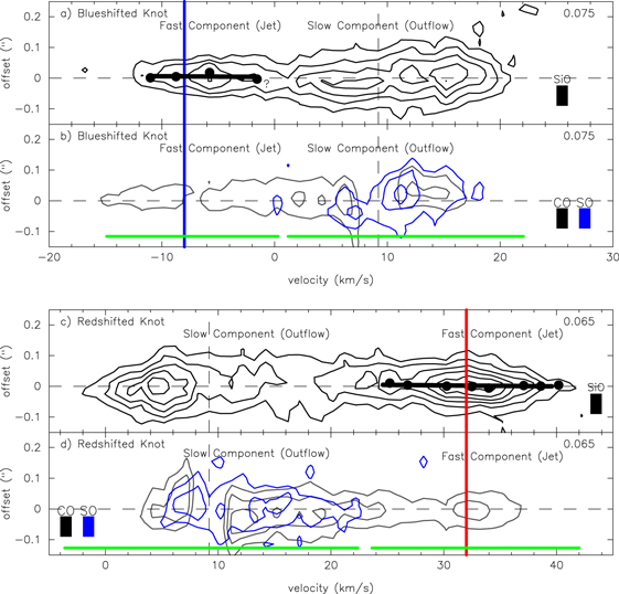
Figure 9. Panels (a) and (c): SiO PV diagrams of knots BK0 and RK0 along cuts perpendicular to the jet axis. The contour levels start at 3σ with a step of 3σ, and σ is ∼2.0 mJy beam−1. Panels (b) and (d): CO (gray contour) and SO (blue contour) PV diagrams of knots BK0 and RK0 along cuts perpendicular to the jet axis. The contour levels start at 3σ with a step of 3σ for CO and 2σ with a step of 2σ for SO. σ is ∼2.0 mJy beam−1 and ∼1.9 mJy beam−1 for CO and SO, respectively. The blue vertical line marks the mean velocity of the jet on the blueshifted side, which is −8 km s−1. The red vertical line marks the mean velocity of the jet on the redshifted side, which is 32 km s−1. The filled circles dot the peak positions, and the thick line roughly connects these peaks. The numbers in the upper right corner indicate the distance from the source to the zero position of the cuts. The green segments denote the velocity range of the slow component defined by the SO emission.
Download figure:
Standard image High-resolution imageIn addition, SiO and CO also trace a fast component (∼−15 to 0 km s−1 in the blueshifted knot and ∼24 to 42 km s−1 in the redshifted knot), allowing us to search for jet rotation. This fast component, with the central velocity close to the velocity of the jet (as discussed in Section 3.5), traces the jet itself. However, no clear velocity gradient can be seen in these knots at our current resolution.
3.5. Kinematics along the Jet Axis
To study the kinematics along the jet axis, we present PV diagrams cut along the jet axis in CO and SiO (Figure 10). The PV structures in CO and SiO are roughly the same. In addition, the PV structures on the blue- and redshifted side are also roughly the same. Note that in Figure 10(a), the roughly linear structure seen in CO (red contours) on the right side of the jet (roughly at x offsets from −26 to −40) that appears on the other side of the main wiggle is the outflow structure around the jet.
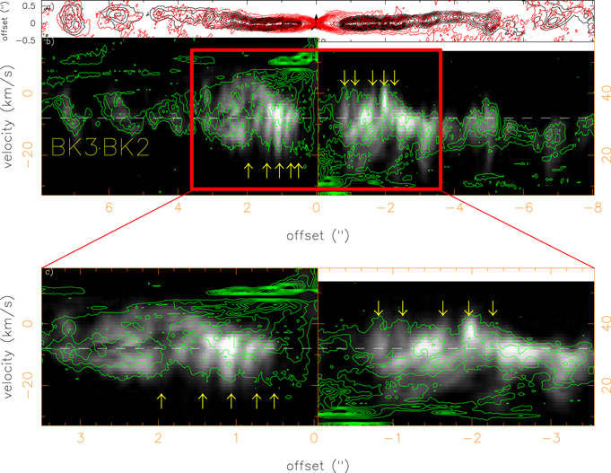
Figure 10. Panel (a): SiO (black contour) and CO (red contour) intensity maps. For SiO, the contour levels start at 3σ with a step of 6σ, and σ is ∼0.2 mJy beam−1. For CO, the contour levels start at 3σ with a step of 6σ, and σ is ∼0.1 mJy beam−1. The asterisk denotes the position of central source. Panels (b) and (c): SiO (gray color) and CO (green contour) PV diagram. For CO, the contour levels start at 3σ with a step of 6σ, and σ is ∼0.95 mJy beam−1. The horizontal dashed white lines mark the mean velocities, which are −8 km s−1 on the blueshifted side and 32 km s−1 on the redshifted side. The yellow arrows denote the positions of the subknots.
Download figure:
Standard image High-resolution imageThe knotty structures (knots BK1a, BK2, and BK3) on the blueshifted side are clear. Previously, Jhan & Lee (2016) derived the distance for an internal shock to fully form, which is  26 updated for the new proper motion measurement, where vj
∼ 102 km s−1 is the jet velocity, Δv ∼ 30 km s−1 is the amplitude of the velocity variation (based on the velocity range of knot BK1), and P ∼ 20 yr is the period of the velocity variation (based on the mean interknot spacing and the proper motion). Thus, these knot structures should be produced by fully formed internal shocks. Their PV structures are all linear with the slow material ahead of the fast material. This indicates that when the fast material catches up with the slow material, it will form an internal working surface between them (see Figure 1 in Suttner et al. 1997). Figure 12 shows that the PV structure of the knot BK3 shows several peaks. As discussed below, these peaks likely point out the positions of the backward (peaks at higher velocity) and forward (peaks at lower velocity) shock, and the internal working surface (point at medium velocity) formed in the knot (Raga et al. 1990; Stone & Norman 1993; Suttner et al. 1997; Lee & Sahai 2004; Jhan & Lee 2016).
26 updated for the new proper motion measurement, where vj
∼ 102 km s−1 is the jet velocity, Δv ∼ 30 km s−1 is the amplitude of the velocity variation (based on the velocity range of knot BK1), and P ∼ 20 yr is the period of the velocity variation (based on the mean interknot spacing and the proper motion). Thus, these knot structures should be produced by fully formed internal shocks. Their PV structures are all linear with the slow material ahead of the fast material. This indicates that when the fast material catches up with the slow material, it will form an internal working surface between them (see Figure 1 in Suttner et al. 1997). Figure 12 shows that the PV structure of the knot BK3 shows several peaks. As discussed below, these peaks likely point out the positions of the backward (peaks at higher velocity) and forward (peaks at lower velocity) shock, and the internal working surface (point at medium velocity) formed in the knot (Raga et al. 1990; Stone & Norman 1993; Suttner et al. 1997; Lee & Sahai 2004; Jhan & Lee 2016).
Within a distance of 26, subknots of knots BK1 and RK1 can be seen on the blue- and redshifted sides in the intensity maps (Figure 10(a)). Although they are hard to identify in the PV diagrams, we can still see four to five cycles of velocity variations, with a variation range of about 25–30 km s−1 for these subknots, consistent with the result in Lee et al. (2009).
Figure 10(c) zooms into the continuous structures, showing the subknot structures in them. The distance between two subknots is about 03, thus the period of the subknot ejection is about 4.5 yr, using a jet velocity of 102 km s−1. Therefore, using the same formula, the distance for an internal shock to fully form in the subknots is ∼06. This is consistent with our observations, which show CO but no SiO emission between 01 to 05 and −01 to −05 because the shocks have not formed yet, and thus no SiO emission can be detected. This result is also aligned with a previous simulation that suggested that a velocity variation with a shorter period is needed to produce the bright emission in the continuous SiO structure near the source (Moraghan et al. 2016). In summary, the PV diagrams suggest at least two different variation periods: one to form the subknot regions near the central source, and the other to form the knotty structure farther downstream the jet.
3.6. Column Density and SiO and SO Abundances in Knot BK3
The column density of knot BK3 can be estimated from the CO emission. Assuming that the CO emission is in local thermal equilibrium and optically thin, and the abundance of CO relative to H2 is ∼4 × 10⁻⁴, as if the CO gas is formed via gas-phase reactions in an initially atomic jet (Glassgold et al. 1991), the column density of the knot in H2 is N ∼ 5.6 × 1020 cm−2. Because the brightness temperature is ∼90 K, we assume the excitation temperature to be 200 K, as adopted in Lee et al. (2010). This excitation temperature is slightly lower than the kinetic temperature derived from the CO emission in much higher transitions in the far-infrared, which was found to be ≳250 K (Giannini et al. 2001). Then, the (two-sided) mass-loss rate of the jet can be given by  ∼ 1.13 × 10⁻⁶
M⊙ yr−1, where N,
∼ 1.13 × 10⁻⁶
M⊙ yr−1, where N,  , and b are the column density of the jet, the mass of the H2 molecule, and the beam size perpendicular to the jet axis (assuming that the size of the jet beam is ∼04, ∼128 au, discussed in Section 4.2), respectively. This mass-loss rate is consistent with the previous measurement (Lee et al. 2010) after adjustment for the new proper motion.
The SiO and SO abundances in knot BK3 can be derived from their column densities and that of H2. The kinetic temperature was found to be 300−500 K in knots BK1 and RK1 (Hirano et al. 2006). Because knot BK3 is farther away and expands, its excitation temperature should be lower and is thus assumed to be 300 K. This excitation temperature of SiO and SO is higher than that of CO because both emissions seem to trace stronger shocks than the CO emission does. When we assume that both emissions are optically thin, the SiO and SO column density are ∼7.9 × 1014 cm−2 and ∼1.0 × 1014 cm−2, resulting in SiO and SO abundances of ∼1.4 × 10⁻⁶ and ∼1.8 × 10⁻⁷, respectively. Note that the abundance of SiO in quiescent molecular clouds is ≤1 × 10⁻¹¹ (Ziurys et al. 1989), and the abundance of SO in cold quiescent clouds (cores) is ∼5 × 10⁻⁹ (Ohishi & Kaifu 1998). This means that both SiO and SO are highly enhanced by shocks in the knot.
4. Discussion
4.1. Wiggle Structure and Protobinary?
As mentioned in Section 3.3, the orbiting jet source model could still fit our current observation with some deviations. Because this model can also fit the wiggle structure farther out in another three epochs over a period of 9 yr, we believe that the model is roughly correct but needs some refinement. Comparing our observational results in Figure 5(b) to 2008 SMA observations in Figure 5(c) at the same resolution, we found that the peaks of the knots (knot BK1a, BK2, and BK3) in our ALMA observations deviate to the north from the model, with little flux detected in the south. This deviation does not appear in the SMA observations, in which the peaks of the knots are aligned with the model.
One possible reason is that our ALMA observation results might miss some flux, so that some flux of the knots is missing. The maximum recoverable size is ∼075, and the size of the knots is ∼1'', so the structures of the knots may not be fully observed. Therefore the apparent peaks of the knots may deviate to the north from the model, but we are not sure how and to what extent the missing flux affects our results. Observations with more complete UV coverage are needed to confirm this possibility.
It is also possible that the structures of the knots do deviate to the north from the model. In the orbiting jet source model (Lee et al. 2010), the orbit of the jet source was assumed to be circular. However, because this reflection-symmetric wiggle is likely due to an orbital motion of the jet source in a binary system (Lee et al. 2010), it is possible that the orbit is not perfectly circular. It may be elliptical so that the model may under- or overestimate the trajectories at different distances (González & Raga 2004). In the high-resolution observation, the peak positions of the knots therefore cannot be fitted exactly by the model. Nonetheless, because the binary separation in this model is ∼4.6 au (Lee et al. 2010), further observations at higher resolution are also needed to confirm or refute whether a binary system exists.
4.2. Backward and Forward Shocks and Sideways Ejection
As mentioned in Section 3.5, it takes time (or distance as the jet propagates) to fully form internal shocks in knots and subknots, and the corresponding distances in our case are about 26 and 06, respectively. Therefore we expect to see shock structures, including backward and forward shocks and sideways ejection in the knots and subknots, after these distances. Because subknots are not spatially resolved, we focus on the knots here.
Figure 11 summarizes the forward and backward shocks, internal working surface, sideways ejection, and their PV structures in schematic diagrams (Raga et al. 1990; Stone & Norman 1993; Suttner et al. 1997; Lee & Sahai 2004; Jhan & Lee 2016). When we use the cut perpendicular to the jet axis (Figure 11(b)), we can see a hollow elliptical PV structure that is due to the expanding bow-shock structure. At the center of this elliptical PV structure, we can see a filled elliptical PV structure that arises from the jet beam with sideways ejection. In the cut along the jet axis (Figure 11(c)), we can see a zig-zag PV structure containing a forward shock (low velocity), a backward shock (high velocity), an internal working surface (in the middle; Lee & Sahai 2004), and an elliptical PV structure for the sideways ejection extents in the middle.
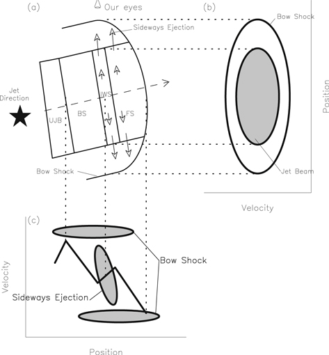
Figure 11. Panel (a): Schematic diagram showing the structure of an internal shock, which consists of an unshocked jet beam (UJB), a backward shock (BS), a forward shock (FS), an internal working surface (IWS), and sideways ejection, for a knot. Panel (b): Simplified PV diagram along a cut perpendicular to the jet axis, illustrating how the bow shock would manifest itself in the diagram; see also Figure 26 in Lee et al. (2000). Panel (c): Simplified PV diagram cut along the jet axis, illustrating how the velocity structure in the knot changes with position; see also Figures 3 and 4 in Raga et al. (1990), Figure 2 in Suttner et al. (1997), and Figure 8 in Lee & Sahai (2004).
Download figure:
Standard image High-resolution imageKnot BK3 appears to be a bow-like structure and is at a greater distance than 26. It can therefore be used to study the shock structure. Figure 12(a) shows a SiO PV diagram of knot BK3 cut along the jet axis through the peak position. We can see a zig-zag PV structure consisting of forward (low-velocity) and backward (high-velocity) shock and internal working surface (in the middle), as discussed above. There are other components in the area of the internal working surface (circled by a red ellipse and labeled "sideways ejection"), and these components may be due to sideways ejection. To make it clearer, Figure 12(b) is a SiO PV diagram of knot BK3 along a cut perpendicular to the jet axis through the peak position, and it shows an elliptical PV structure that can be attributed to a bow-shock structure produced by sideways ejection. Comparing Figures 12(a) and (b) (cut through the same reference central point, but different directions), we conclude that the additional PV component (circled in Figure 12(a)) corresponds to the PV structure of the sideways ejection. Furthermore, the emission inside the elliptical PV structure in Figure 12(b) is the PV structure of the internal working surface (in the jet beam itself), as discussed above. We also calculated that the PV structure of the sideways ejection along the jet axis would be  ∼ 02 in extent, where the width of the knot W ∼ 1'' and the inclination angle i ∼ 11°. This extent agrees with that seen in Figure 12(a) for the region labeled "sideways ejection". In our case, the knot can therefore be resolved into backward and forward shocks plus sideways ejection. A model illustration of these shock structures is given in the next section.
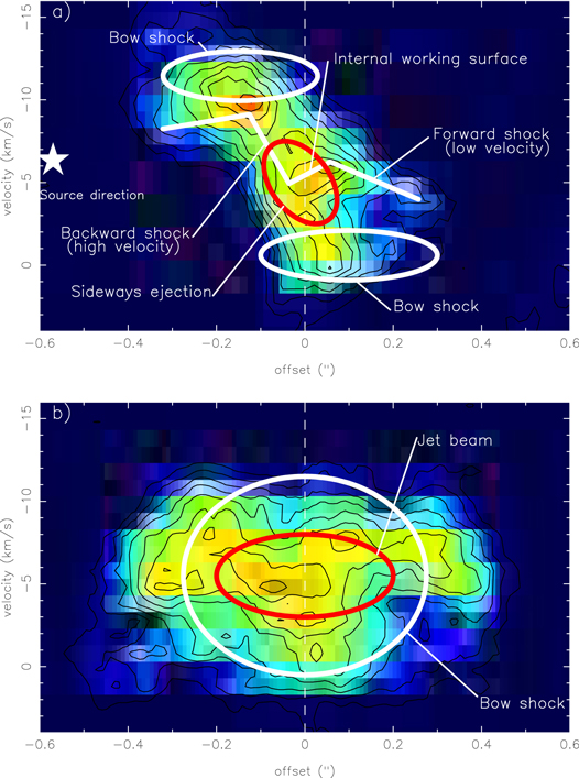
Figure 12. Panel (a): SiO PV diagram of knot BK3 cut along the jet axis. The contour levels start at 3σ with a step of 3σ, and σ is ∼0.95 mJy beam−1. Panel (b): SiO PV diagram of knot BK3 cut perpendicular to the jet axis. The outer white circle denotes the contribution of the sideways ejection, and the inner white circle denotes the contribution of the jet beam.
Download figure:
Standard image High-resolution imageNote that the PV structure of the sideways ejection at different inclinations can be different due to the projection effect. For example, the IRAS 04166+2706 jet has a high inclination angle of ∼52°, and the PV structure becomes a sawtooth pattern (Santiago-García et al. 2009; Tafalla et al. 2017), whereas HH 212 has a very low inclination angle of ∼4°, and the PV structure becomes arc-like (Lee et al. 2015).
4.2.1. Illustrative Model for Shock Structures in Knot BK3
Here we presented a simple kinematic model to illustrate the shock structures in knot BK3 in more detail. As shown in Figure 11, this model has two components, a jet beam and a bow-shock structure. This jet beam consists of an unshocked jet beam (UJB), a backward shock (BS), an internal working surface (IWS), and a forward shock (FS), mimicking an internal shock produced in pulsed-jet simulations (Raga et al. 1990; Suttner et al. 1997; Lee & Sahai 2004). The velocity structure in the jet beam has two components; one is along the jet axis, and the other is perpendicular to the jet axis for the sideways ejection (see Figure 16). The velocity gradients along the jet axis are therefore assumed to roughly match the observation. These velocity gradients are also expected for an internal shock produced in pulsed-jet simulations (Raga et al. 1990; Suttner et al. 1997; Lee & Sahai 2004). On the other hand, the velocity structure in the bow-shock structure (see Figure 17) is adopted from the jet-driven bow-shock model (Ostriker et al. 2001). The resulting PV diagrams are presented in Figure 13. In the PV diagram cut along the jet axis (Figure 13(a)), we see four linear structures as marked by the white lines, arising from the unshocked jet beam, the backward shock, the internal working surface, and the forward shock, respectively. They are roughly consistent with the observation. The sideways ejections are mostly from the internal working surface, causing a spread in velocity there, as marked by the red ellipse in Figure 13(a). The PV structures marked by the white ellipses are from the bow-shock structure, with the upper (more blueshifted) one from the near side and the lower (less blueshifted) one from the far side. They are also roughly similar to those seen in the observation. Their intensity peaks are also at roughly the same locations as those seen in the observations. In the PV diagram, two components lie along a cut perpendicular to the jet axis (Figure 13(b)): one is an elliptical PV structure from the expanding bow-shock structure, and the other is a filled ellipse (marked by the red ellipse) from the jet beam that has a sideways ejection. These features are also similar to those seen in the observation.
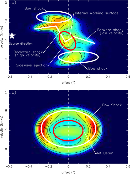
Figure 13. Same as Figure 12, but derived from the radiative-transfer model discussed in the Appendix.
Download figure:
Standard image High-resolution image4.3. Relations between the SiO, CO, and SO Layers
Figure 14 shows the PV diagrams in SiO, CO, and SO of the fully formed knot BK3. The CO and SO PV structures are roughly the same, as shown in Figures 14(b) and (d). However, the PV structures of the CO emission in Figures 14(a) and (c) only show a part of the PV structure of the SiO emission. These missing parts of the CO PV structures could be due to different emission lines tracing different layers. According to Figure 14(c), PV structures of CO emission do not show the redshifted part of elliptical PV structures (due to the expanding shell produced by the sideways ejection). This could be explained if the SiO layer in the bow shock (as shown in the dark gray layer in Figure 15(a)) extends farther out than the CO layer (as shown in the light gray layer in Figure 15(a)). Therefore, the cut inclined to the jet axis by 79 (=90 − 11) degree used in our PV diagrams does not go through the expanding CO shells (see the dotted curve in Figure 15(a)) on the far side of the knot (closer to the central source). This phenomenon may be due to these two lines tracing different densities. The critical density of the SiO(J = 8–7) transition is ∼108 cm−3 (Lee et al. 2009), and that of CO(J = 3–2) is ∼105 cm−3. So CO may trace the low-density part of the bow shock (Figure 15(b)), and the SiO layer traces the higher density and outer bow shock (see the dark gray layer in Figure 15(a)). This phenomenon also appears in HH 212 (Lee et al. 2015), but we do not see a clear extension of SiO and CO in our emission maps (higher resolution observations are needed to distinguish it).

Figure 14. Panel (a): SiO (black contour) and CO (red contour) PV diagram of knot BK3 cut along the jet axis. For SiO, the contour levels start at 3σ with a step of 3σ, and σ is ∼0.95 mJy beam−1. For CO, the contour levels start at 3σ with a step of 3σ, and σ is ∼1 mJy beam−1. Panel (b): SO (black contour) and CO (red contour) PV diagram of knot BK3 cut along the jet axis. For SO, the contour levels start at 3σ with a step of 3σ, and σ is ∼1 mJy beam−1. Panel (c): SiO (black contour) and CO (red contour) PV diagram of knot BK3 along a cut perpendicular to the jet axis. Panel (d): SO (black contour) and CO (red contour) PV diagram of knot BK3 along a cut perpendicular to the jet axis.
Download figure:
Standard image High-resolution image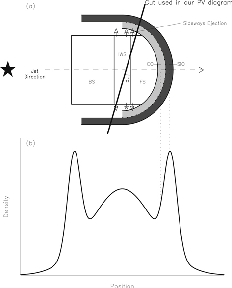
Figure 15. Panel (a): Schematic diagram showing the detailed structures of sideways ejection and SiO (dark gray) and CO (light gray) layers. Panel (b): Simplified position to number density diagram cut along the jet axis, illustrating the change in density with position; see also Figure 2 in Suttner et al. (1997), Figure 8 in Lee & Sahai (2004), and Figure 7 in Lee et al. (2015).
Download figure:
Standard image High-resolution image5. Conclusions
We have studied the properties of the HH 211 jet in the CO(J = 3–2), SiO(J = 8–7), and SO(NJ = 89–78) lines at high resolution with ALMA. Our conclusions are listed below.
- 1.SiO traces the jet. CO and SO trace the jet at high velocity and the outflow shell at low velocity.
- 2.With our ALMA and 2008 SMA observations, we measured the proper motion of eight knots, four on either side in the inner jet. The proper motion of these knots is roughly the same (∼102 km s−1), and consistent with previous measurements in the outer jet.
- 3.In our high-resolution observation, we still see the reflection-symmetric wiggle of the jet, and the orbiting jet source model still fits the trend of the wiggle. However, the knot peaks show some deviations from the model.
- 4.The PV diagrams obtained along the jet axis indicates that the jet continuously ejects material, with two small periodical variations in velocity. The subknot structures are produced by a velocity variation with a shorter period of the two. This also explains why there is no SiO emission between 01 to 05 and −01 to −05.
- 5.The PV diagrams of a fully formed knot BK3 show a backward and a forward shock and sideways ejection. In knot BK3, the SiO traces the high-density outer layer of the bow shock, while CO and SO trace the low-density inner layers of the bow shock.

Figure 16. Panel (a): Schematic diagram showing the detailed structures of jet beam, where UJB, BS, IWS, and FS stand for the unshocked jet beam, the backward shock, the internal working surface, and the forward shock, respectively. Panel (b): Jet velocity profile along the jet axis. Panel (c): Density profile along the jet axis. Panel (d): Maximum sideways ejection velocity profile at the jet boundary.
Download figure:
Standard image High-resolution image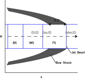
Figure 17. Schematic diagram showing the detailed structures of the jet beam and the bow shock, where BS, IWS, and FS stand for the backward shock, the internal working surface, and the forward shock, respectively.
Download figure:
Standard image High-resolution image
This paper makes use of the following ALMA data: ADS/JAO.ALMA#2015.1.00024.S, ADS/JAO.ALMA#2016.1.00017.S. ALMA is a partnership of ESO (representing its member states), NSF (USA) and NINS (Japan), together with NRC (Canada), MOST and ASIAA (Taiwan), and KASI (Republic of Korea), in cooperation with the Republic of Chile. The Joint ALMA Observatory is operated by ESO, auI/NRAO and NAOJ. We acknowledge grants from the Ministry of Science and Technology of Taiwan (MoST 107-2119-M-001-040-MY3) and the Academia Sinica (Investigator Award AS-IA-108-M01). We also thank Anthony Moraghan for useful discussion.
Appendix: Shock Model for Knot BK3
As mentioned in Section 4.2.1, we constructed a simple kinematic model to produce the features seen in the observations. We adopted a cylindrical coordinate system, and assumed that the jet propagates along the z-axis (see Figure 16(a)) and has a cylindrical radius Rj = 02.
The jet beam has four components: UJB (unshocked jet beam), BS (backward shock), IWS (internal working surface), and FS (forward shock), with their velocity and density structures in the z-axis shown in Figures 16(b) and (c), respectively. The velocity gradients here follow those expected from the internal shock produced by a periodical variation in the jet velocity (Raga et al. 1990; Suttner et al. 1997; Lee & Sahai 2004).
The jet beam also has a sideways ejection (SE) perpendicular to the z-axis. The sideways ejection is assumed to increase along the R-axis from zero to a maximum value at the jet boundary. The maximum value at the jet boundary is assumed to peak at the internal working surface, and it decreases toward the backward and the forward shocks (Figure 16(d)).
For the bow shock around the jet beam (see Figure 17), we followed the jet-driven bow-shock model reported in Ostriker et al. (2001). The shape of the bow shock is given by

where zbo = 05 is z position of the bow-shock tip (see Figure 17), cs = 8 km s−1 is the isothermal sound speed in the shock, and β = 4 is to account for the effective impulse from the shock, as found in Ostriker et al. (2001).
The velocity structures of the bow-shock structure are
where vs = 14 km s−1 is the shock velocity to roughly match the observation.
The bow-shock structure has a thickness of 03. Its density is assumed to be

,where zo is a constant. With this assumption, the density is highest at z = 0, which is a location aligned with the internal working surface, to match the observation.