


Abstract
Long-period Mira variable stars are considered to have relatively high initial masses and may be potentially useful as tracers of spiral arm structure of the Milky Way. From 2004 to 2017, we monitored long-period Mira candidates selected from the IRAS color–color diagram in the near-infrared K' band. As an initial result of this study, we found 108 Mira variables and determined their periods, mean magnitudes, and amplitudes. Most of them are located between 0° and 90° in Galactic longitude. The peak of their period distribution is at around 500 days, which is longer than the typical value for Mira variables selected in optical surveys. Distances to our Mira variables have also been estimated using the period–luminosity relation (PLR) in 3.4 μm with the help of a three-dimensional map of interstellar extinction. While the Ks-band PLR has a large scatter at longer periods (log P > 2.6), the PLR based on the Wide-field Infrared Survey Explorer 3.4 μm data has a much smaller scatter. We compare the spatial distribution of our sample to the spiral arms in the literature, and discuss the possible association of the long-period Mira variables with the spiral arms although the limited spatial coverage and the limited distance accuracy of the current sample prevent us from drawing a firm conclusion.
Export citation and abstract BibTeX RIS
1. Introduction
From our perspective within the Galactic disk, it is difficult to establish the large-scale and detailed structure of the Milky Way. Many studies have been done using methods of estimating distances of various tracers of the Galactic structures, for example, H i gas and star-forming regions (SFRs; Kerr 1961). Since the Milky Way is composed of stars and gas, it is necessary to study the distribution of both components to obtain a complete view of Galactic structure. Regarding the stellar component, different tracers should be used for different stellar populations; for example, red clump stars are suitable tracers of old stellar populations in the bulge (e.g., Weiland et al. 1994; Lopez-Corredoira et al. 1997). Mira variables are also good tracers of the bulge, and several previous works investigated their distribution (e.g., Matsunaga et al. 2005; Catchpole et al. 2016). On the other hand, the spiral arms are typically traced by using high-mass SFRs (HMSFR, Burns et al. 2014; Reid et al. 2014, etc.) and classical Cepheids (Gozha & Marsakov 2013; Dambis et al. 2015). In the effort of revealing the spiral arm and the disk structure of the Milky Way, young tracers are important. However, they are also rarer relative to old objects, which tends to prevent us from establishing a detailed map of a young stellar population. In this work, we focus on Mira variables which are abundant throughout the Milky Way; they are more numerous than HMSFRs by a few orders of magnitude (LPV catalog in Milky Way; e.g., Watson et al. 2006; Mowlavi et al. 2018) (HMSFR, Reid et al. 2014).
Mira variables are a class of late-type and long-period variable (LPV) stars that populate the coolest and most luminous part of the asymptotic giant branch (AGB). They have long pulsation periods (Period > 100 days) and large amplitude variations (ΔV > 2.5 mag, ΔK > 0.4 mag). The AGB is the final evolutionary phase of low- to intermediate-mass (1–8 M⊙) stars before the start of the envelope ejection (Habing & Olofsson 2003). The period of Mira variables is a good indicator of its age and initial mass, Mi (Feast & Whitelock 2000; Feast 2008); the shortest period Mira variables (some of which are found in metal-rich globular clusters) are very old with Mi < 1 M⊙, while the bulk of Mira variables in the solar neighborhood with log P ∼ 2.5 are ∼7 Gyr old. An age of ∼3 Gyr has been estimated to be log P ∼ 2.65 and longer period Mira variables (including OH/IR stars which typically are also long-period Mira variables) are even younger (∼100 Myr) (Catchpole et al. 2016). Due to their short lifetime, we can reasonably assume that the longer period Mira variables are still located close to the spiral arms where they formed. Furthermore, Mira variables are bright at infrared wavelengths meaning they can be seen through the Galactic disk.
The period–luminosity relation (PLR) of Mira variables has been widely used as a distance indicator since it was established by Glass & Evans (1981) and Feast et al. (1989). As discovered by Wood (2000), AGB variables lie on several parallel sequences in the K band PL diagram, where each sequence corresponds to a particular pulsation mode. Mira variables have larger amplitudes than semi-regular variables and mostly fall on the PL relation corresponding to the fundamental pulsation mode (the sequence C in Wood 2000). However, Mira variables with longer periods (P > 400 days) tend to have thick circumstellar dust shells and are fainter than the PLR of shorter period Mira variables due to the circumstellar extinction. (Whitelock et al. 1991; Glass et al. 1995; Matsunaga et al. 2009). For example, the Ks band PLR shows a large scatter with many long-period Mira variables getting fainter (Ita & Matsunaga 2011). In contrast, the 3.6 μm PLR of Mira variables for the Large Magellanic Cloud (LMC) presented in the same paper has a much tighter relation which would be more useful for determining the distances of longer period Mira variables. In the present paper, we report an analysis of the monitoring data in the near-infrared K' band, and derived parameters for 108 Mira variables. We selected Mira variable candidates from the IRAS point-source catalog (PSC), to isolate long-period candidates which are typically young in the IIIa and IIIb regions of the IRAS color–color diagram (van der Veen & Habing 1988). We combined these observations with the 2MASS data and the Wide-field Infrared Survey Explorer (WISE) data, to determine the spatial distribution of long-period Mira variables and compare them with the spiral arm structure.
2. Sample Selection and Observation
2.1. Sample Selection
We selected bright infrared sources that satisfy the following criteria as candidates of the long-period Mira variables from the IRAS PSC (Neugebauer et al. 1984). First, sources with decl. > −25° were selected considering the latitude of our observatory site, Kagoshima, located at a latitude of 31 5 north. Second, targets needed to be bright in all bands; 12, 25, and 60 μm (flux density quality = 3 in the IRAS PSC). Third, targets are required to be located in the IIIa or IIIb regions on the IRAS color–color diagram (van der Veen & Habing 1988). The position of the IIIa and IIIb regions are indicated in Figure 1, together with the distribution of the 108 Mira variables examined in this paper. The IIIa and IIIb regions lie around the most evolved phase of the sequence of dust shell evolution of AGB (van der Veen & Habing 1988). Therefore, the stars located in these regions are likely to have a longer period. There are 2300 for the IIIa and 280 for IIIb, which satisfy the above three criteria.

Figure 1. Distribution of 108 sources for which we determined their periods in this paper, on the IRAS color−color diagram. The solid lines correspond to the border lines of regions indicated in van der Veen & Habing (1988).
Download figure:
Standard image High-resolution imageFigure 2 shows the l − b diagram of sources satisfying the criteria including those for which we report distances in this paper. There is a gap around l = 80°. There are few IRAS sources in this area because IRAS observation was not performed in this area. In this paper, we report on 108 sources for which accurate periods were determined so far.
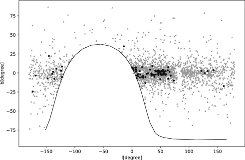
Figure 2. The l − b distribution of the IRAS sources. Gray marks (triangle) indicate all the sources that satisfy our criteria. Black marks are the sources for which we determined their distance in this paper. The solid line corresponds to decl. = −25°.
Download figure:
Standard image High-resolution image2.2. Observation
Our monitoring observations were carried out at Iriki observatory operated by Kagoshima University (Chibueze et al. 2016), Japan, since 2003. A near-IR camera with a 512 × 512 HgCdTe array detector attached to a 1 m telescope yielding 5 38 × 538 field of view (0
 63 pixel scale) was used. The typical seeing measurement at the Iriki observatory is 15. Monitoring observations in the K' band were performed in the fields centered on the position of the selected IRAS sources. Each set of observations consists of five exposures at slightly dithered positions with an exposure time of 1–12 s. We adjusted the exposure time depending on the sky background level, and the brightness of the target and reference stars in the same field. Stars brighter than K' ∼ 6.5 mag would be saturated at the best focus position, and therefore we observed such bright sources with the focus off. For targets for which no reference star was found in the same field of view, we also observed the standard stars listed in Elias et al. (1982) on the same night. We searched for the counterparts of IRAS objects in the 2MASS image. In many cases, the bright near-infrared counterparts were found near the IRAS position. The coordinates of the 108 sources in Table 1 are based on the 2MASS catalog (J2000.0).
Table 1. Observable Characteristics of Our Samples
| IRASname | R.A. [h m s] (J2000) | Decl. [d m s] (J2000) | Period (days) | Amplitudes (Kmag) | K'(mag) | W1 (mag) | Aw1 (mag) | Distance (kpc) | Z (kpc) |
|---|---|---|---|---|---|---|---|---|---|
| IRAS 00361+6515 | 00 39 03.61368 | +65 32 07.2204 | 650 | 1.89 | 9.75 | 6.36 | 0.28 | 14.42 | 0.68 |
| IRAS 01304+6211 | 01 33 51.21048 | +62 26 53.2032 | 759 | 1.18 | 6.90 | 3.83 | 0.19 | 5.37 | 0.00 |
| IRAS 02173+6322 | 02 21 11.90064 | +63 36 18.2196 | 698 | 1.68 | 8.28 | 5.91 | 0.14 | 13.29 | 0.57 |
| IRAS 03385+5927 | 03 42 39.99072 | +59 36 59.9652 | 618 | 1.93 | 7.43 | 3.79 | 0.14 | 4.50 | 0.28 |
| IRAS 03453+3207 | 03 48 32.31240 | +32 16 43.7916 | 409 | 1.02 | 4.36 | 3.54 | 0.06 | 2.87 | −0.85 |
| IRAS 04312+1007 | 04 33 58.38048 | +10 13 52.6872 | 425 | 0.57 | 4.10 | 3.44 | 0.04 | 2.86 | −1.18 |
| IRAS 05552+1720 | 05 58 07.50696 | +17 20 58.4772 | 520 | 1.04 | 5.88 | 4.58 | 0.10 | 5.64 | −0.34 |
| IRAS 06228-0244 | 06 25 21.64896 | −02 46 37.9128 | 412 | 1.15 | 4.68 | 3.98 | 0.05 | 3.56 | −0.44 |
| IRAS 06418-1317 | 06 44 08.23968 | −13 20 08.9232 | 347 | 0.88 | 6.39 | 6.15 | 0.05 | 8.27 | −1.10 |
| IRAS 06583-0655 | 07 00 44.51832 | −06 59 43.5984 | 431 | 0.97 | 4.60 | 4.21 | 0.11 | 4.00 | −0.08 |
| IRAS 07109-0713 | 07 13 23.20944 | −07 18 33.6708 | 316 | 1.30 | 6.93 | 5.82 | 0.07 | 6.47 | 0.17 |
| IRAS 07153-2411 | 07 17 28.17912 | −24 17 13.5852 | 495 | 2.06 | 5.38 | 3.89 | 0.03 | 4.05 | −0.39 |
| IRAS 07372-1036 | 07 39 39.53064 | −10 43 05.4588 | 467 | 0.86 | 4.36 | 3.76 | 0.02 | 3.65 | 0.36 |
| IRAS 07434-1847 | 07 45 40.92408 | −18 54 29.1744 | 678 | 1.39 | 11.51 | 5.59 | 0.05 | 11.67 | 0.58 |
| IRAS 08066-1719 | 08 08 56.45328 | −17 28 38.8452 | 510 | 1.57 | 6.97 | 3.73 | 0.01 | 3.89 | 0.56 |
| IRAS 08116+0843 | 08 14 18.76224 | +08 34 24.4704 | 263 | 0.96 | 4.65 | 4.65 | 0.00 | 3.31 | 1.26 |
| IRAS 15106-1532 | 15 13 25.77504 | −15 43 59.5416 | 268 | 1.38 | 8.66 | 7.25 | 0.01 | 11.07 | 6.35 |
| IRAS 17179-2452 | 17 21 01.47744 | −24 55 50.1492 | 597 | 2.03 | 10.64 | 6.93 | 0.15 | 18.38 | 2.17 |
| IRAS 17259-2326 | 17 28 59.79696 | −23 28 38.9676 | 648 | 1.90 | 8.17 | 5.77 | 0.19 | 11.39 | 1.20 |
| IRAS 17287-1955 | 17 31 40.98336 | −19 58 07.7268 | 562 | 2.01 | 10.37 | 6.86 | 0.17 | 16.71 | 2.16 |
| IRAS 17292-2408 | 17 32 16.53480 | −24 10 56.6256 | 682 | 2.02 | 7.95 | 5.55 | 0.19 | 10.78 | 0.95 |
| IRAS 17304-1933 | 17 33 22.14840 | −19 35 52.2348 | 547 | 1.46 | 7.60 | 5.72 | 0.15 | 9.73 | 1.24 |
| IRAS 17324-1918 | 17 35 23.78904 | −19 20 47.0508 | 610 | 1.40 | 8.15 | 5.16 | 0.10 | 8.49 | 1.04 |
| IRAS 17350-2413 | 17 38 08.84976 | −24 14 49.2756 | 542 | 2.46 | 10.63 | 7.14 | 0.16 | 18.46 | 1.25 |
| IRAS 17411-2029 | 17 44 04.88088 | −20 30 32.2920 | 561 | 2.48 | 9.25 | 6.06 | 0.15 | 11.66 | 0.95 |
| IRAS 17476-2036 | 17 50 35.63016 | −20 37 43.6152 | 432 | 1.44 | 8.42 | 6.24 | 0.22 | 9.72 | 0.56 |
| IRAS 17521-2201 | 17 55 07.46544 | −22 01 31.6128 | 850 | 3.24 | 12.45 | 7.69 | 0.27 | 33.87 | 1.01 |
| IRAS 17531-0940 | 17 55 53.14608 | −09 41 20.6448 | 682 | 2.34 | 7.34 | 4.68 | 0.16 | 7.33 | 0.98 |
| IRAS 18033-1551 | 18 06 12.86976 | −15 51 06.3072 | 475 | 1.56 | 8.48 | 6.38 | 0.27 | 11.04 | 0.48 |
| IRAS 18117-2022 | 18 14 42.51720 | −20 21 10.2060 | 633 | 2.20 | 8.49 | 4.85 | 0.39 | 6.67 | −0.17 |
| IRAS 18154-2257 | 18 18 30.18408 | −22 56 01.3704 | 708 | 2.06 | 8.40 | 6.12 | 0.13 | 14.96 | −0.90 |
| IRAS 18211-1712 | 18 24 05.21208 | −17 11 13.8048 | 457 | 1.86 | 8.31 | 5.14 | 0.21 | 6.18 | −0.21 |
| IRAS 18216+0634 | 18 24 03.72288 | +06 36 25.8984 | 830 | 2.04 | 8.70 | 5.19 | 0.03 | 11.73 | 1.85 |
| IRAS 18219-2140 | 18 24 57.70008 | −21 38 51.4900 | 703 | 2.23 | 9.86 | 5.091 | 0.09 | 9.40 | −0.69 |
| IRAS 18282-2458 | 18 31 19.11480 | −24 56 08.0160 | 394 | 0.98 | 9.47 | 6.60 | 0.06 | 11.38 | −1.38 |
| IRAS 18307+0102 | 18 33 15.25128 | +01 04 39.0828 | 494 | 1.19 | 6.15 | 4.65 | 0.30 | 5.07 | 0.40 |
| IRAS 18351-1947 | 18 38 08.97120 | −19 44 28.2300 | 494 | 1.34 | 4.83 | 4.02 | 0.06 | 4.25 | −0.45 |
| IRAS 18382-1338 | 18 41 04.72152 | −13 35 52.0044 | 676 | 1.73 | 8.30 | 5.60 | 0.17 | 11.04 | −0.75 |
| IRAS 18394-1600 | 18 42 22.31184 | −15 57 05.6988 | 489 | 1.31 | 7.09 | 4.83 | 0.08 | 6.06 | −0.55 |
| IRAS 18404-0645 | 18 43 07.20960 | −06 42 40.1400 | 760 | 2.15 | 7.11 | 4.00 | 0.13 | 5.98 | −0.13 |
| IRAS 18418-0415 | 18 44 31.32792 | −04 12 15.8724 | 897 | 2.11 | 8.30 | 5.41 | 0.28 | 12.39 | −0.08 |
| IRAS 18475-1428 | 18 50 22.90104 | −14 24 30.7332 | 590 | 2.20 | 7.90 | 6.15 | 0.10 | 13.03 | −1.43 |
| IRAS 18511-1044 | 18 53 56.07672 | −10 40 40.8072 | 647 | 1.86 | 8.95 | 5.85 | 0.07 | 12.48 | −1.17 |
| IRAS 18522+0032 | 18 54 45.59952 | +00 36 02.1528 | 700 | 2.09 | 8.64 | 5.32 | 0.55 | 8.44 | −0.07 |
| IRAS 18530+0817 | 18 55 25.22304 | +08 21 15.9300 | 745 | 1.47 | 4.96 | 3.41 | 0.30 | 4.13 | 0.21 |
| IRAS 18549+0905 | 18 57 20.81592 | +09 09 40.8816 | 471 | 0.95 | 4.66 | 4.02 | 0.21 | 3.78 | 0.19 |
| IRAS 18556+0003 | 18 58 14.96976 | +00 07 28.5996 | 643 | 1.87 | 8.87 | 6.07 | 0.31 | 12.33 | −0.31 |
| IRAS 18559+0103 | 18 58 31.76232 | +01 07 47.4672 | 771 | 2.31 | 12.78 | 7.50 | 0.27 | 28.50 | −0.53 |
| IRAS 18567+0003 | 18 59 21.17376 | +00 07 26.4324 | 667 | 1.37 | 5.60 | 4.25 | 0.25 | 5.67 | −0.17 |
| IRAS 18585+0900 | 19 00 53.82114 | +09 05 02.7305 | 867 | 1.59 | 5.80 | 3.27 | 0.29 | 4.48 | 0.16 |
| IRAS 19010+1307 | 19 03 21.50832 | +13 12 01.2024 | 843 | 2.48 | 8.20 | 5.87 | 0.18 | 15.16 | 0.90 |
| IRAS 19026+0007 | 19 05 15.99624 | +00 12 18.5652 | 482 | 1.25 | 5.37 | 4.46 | 0.12 | 4.95 | −0.26 |
| IRAS 19031-0035 | 19 05 40.52520 | −00 30 45.6120 | 321 | 1.18 | 9.52 | 6.84 | 0.11 | 10.31 | −0.61 |
| IRAS 19037+0204 | 19 06 18.45264 | +02 09 03.5280 | 580 | 0.86 | 5.95 | 5.18 | 0.24 | 7.67 | −0.31 |
| IRAS 19046+1121 | 19 07 01.79688 | +11 26 10.6692 | 526 | 2.26 | 10.34 | 6.22 | 0.22 | 11.46 | 0.36 |
| IRAS 19068+1127 | 19 09 11.67960 | +11 32 48.1956 | 678 | 1.40 | 5.40 | 4.54 | 0.22 | 6.64 | 0.16 |
| IRAS 19074+0336 | 19 09 54.92112 | +03 41 27.3912 | 612 | 1.37 | 7.36 | 4.70 | 0.18 | 6.67 | −0.28 |
| IRAS 19082+1456 | 19 10 33.33888 | +15 01 11.6616 | 464 | 1.46 | 6.41 | 5.30 | 0.15 | 6.96 | 0.32 |
| IRAS 19087+0323 | 19 11 17.00856 | +03 28 24.3984 | 631 | 1.94 | 7.39 | 4.97 | 0.35 | 7.18 | −0.35 |
| IRAS 19087+1413 | 19 11 05.30352 | +14 18 23.0328 | 536 | 0.89 | 5.14 | 4.04 | 0.09 | 4.55 | 0.18 |
| IRAS 19097+0411 | 19 12 13.21704 | +04 16 54.5664 | 517 | 1.21 | 5.82 | 4.44 | 0.25 | 4.90 | −0.23 |
| IRAS 19126+0648 | 19 15 06.06960 | +06 53 29.0256 | 630 | 2.09 | 11.04 | 6.87 | 0.23 | 18.15 | −0.66 |
| IRAS 19128+1310 | 19 15 07.96872 | +13 16 00.0552 | 817 | 3.43 | 8.38 | 4.79 | 0.26 | 8.64 | 0.13 |
| IRAS 19131+1551 | 19 15 25.06176 | +15 56 32.8848 | 851 | 2.81 | 11.41 | 5.41 | 0.20 | 12.27 | 0.44 |
| IRAS 19136+2055 | 19 15 47.39376 | +21 00 32.5116 | 589 | 1.78 | 9.14 | 6.13 | 0.18 | 12.42 | 0.94 |
| IRAS 19143+1817 | 19 16 33.90949 | +18 22 51.9676 | 415 | 0.95 | 4.04 | 3.52 | 0.15 | 2.76 | 0.14 |
| IRAS 19149+1638 | 19 17 11.55675 | +16 43 54.6222 | 583 | 1.49 | 5.16 | 3.54 | 0.20 | 3.69 | 0.13 |
| IRAS 19151+1456 | 19 17 26.10720 | +15 01 59.0268 | 534 | 1.25 | 5.88 | 4.87 | 0.19 | 6.35 | 0.13 |
| IRAS 19167+1733 | 19 19 00.02040 | +17 38 51.9036 | 497 | 0.88 | 5.48 | 4.35 | 0.29 | 4.47 | 0.16 |
| IRAS 19175+1042 | 19 19 57.26616 | +10 48 09.1440 | 545 | 1.64 | 7.93 | 5.13 | 0.31 | 6.87 | −0.16 |
| IRAS 19176+1939 | 19 19 48.03696 | +19 45 35.8776 | 560 | 1.31 | 6.44 | 5.50 | 0.21 | 8.76 | 0.44 |
| IRAS 19186+0315 | 19 21 11.69976 | +03 20 57.8652 | 497 | 1.82 | 6.15 | 4.65 | 0.12 | 5.55 | −0.49 |
| IRAS 19190+1128 | 19 21 26.68848 | +11 33 56.6100 | 856 | 2.42 | 7.60 | 4.02 | 0.25 | 6.36 | −0.14 |
| IRAS 19190+3035 | 19 20 59.23344 | +30 41 28.6764 | 581 | 1.58 | 8.23 | 5.47 | 0.38 | 8.28 | 1.11 |
| IRAS 19195-1423 | 19 22 22.58256 | −14 18 05.0688 | 425 | 1.36 | 6.42 | 4.75 | 0.03 | 5.26 | −1.20 |
| IRAS 19195+1747 | 19 21 44.11944 | +17 53 09.7080 | 519 | 1.07 | 5.02 | 3.74 | 0.29 | 3.52 | 0.10 |
| IRAS 19202+2009 | 19 22 25.53000 | +20 15 35.4528 | 782 | 1.54 | 5.90 | 4.43 | 0.22 | 7.18 | 0.33 |
| IRAS 19235+1034 | 19 25 56.66640 | +10 40 22.8864 | 540 | 1.29 | 8.07 | 6.99 | 0.18 | 17.13 | −0.80 |
| IRAS 19236+2003 | 19 25 49.34208 | +20 09 13.4424 | 552 | 1.67 | 6.29 | 4.56 | 0.22 | 5.59 | 0.18 |
| IRAS 19237+1430 | 19 26 02.24328 | +14 36 39.2760 | 559 | 1.24 | 4.93 | 3.81 | 0.26 | 3.92 | −0.06 |
| IRAS 19261+1435 | 19 28 28.48488 | +14 41 52.1592 | 633 | 1.80 | 7.95 | 5.97 | 0.41 | 11.09 | −0.25 |
| IRAS 19276+1500 | 19 29 53.85312 | +15 06 48.3912 | 551 | 1.28 | 6.18 | 5.02 | 0.27 | 6.73 | −0.17 |
| IRAS 19282+2253 | 19 30 19.90704 | +23 00 01.0224 | 639 | 1.25 | 5.15 | 4.07 | 0.12 | 5.31 | 0.21 |
| IRAS 19283+1421 | 19 30 38.02152 | +14 27 55.7568 | 468 | 1.39 | 5.94 | 4.06 | 0.24 | 3.78 | −0.12 |
| IRAS 19303+1553 | 19 32 35.87520 | +15 59 41.0712 | 637 | 1.11 | 7.30 | 6.14 | 0.28 | 12.82 | −0.35 |
| IRAS 19305+2410 | 19 32 39.94416 | +24 16 55.9272 | 685 | 1.06 | 5.14 | 4.30 | 0.16 | 6.18 | 0.26 |
| IRAS 19307+1441 | 19 33 04.51344 | +14 48 27.2628 | 574 | 0.95 | 6.14 | 5.37 | 0.25 | 8.27 | −0.32 |
| IRAS 19320+2013 | 19 34 14.17824 | +20 20 02.3856 | 523 | 1.13 | 5.83 | 4.47 | 0.30 | 4.90 | 0.02 |
| IRAS 19333+1918 | 19 35 30.77928 | +19 25 06.4812 | 630 | 1.39 | 4.86 | 3.87 | 0.29 | 4.43 | −0.04 |
| IRAS 19338+1522 | 19 36 10.28304 | +15 28 47.8596 | 303 | 0.99 | 5.06 | 4.56 | 0.16 | 3.36 | −0.15 |
| IRAS 19344+2114 | 19 36 37.25640 | +21 21 13.6728 | 474 | 1.99 | 6.67 | 4.79 | 0.29 | 5.22 | 0.02 |
| IRAS 19347+2755 | 19 36 44.55072 | +28 01 58.3428 | 632 | 1.63 | 7.21 | 5.95 | 0.11 | 12.57 | 0.75 |
| IRAS 19349+1657 | 19 37 12.79200 | +17 03 47.3832 | 543 | 1.26 | 6.52 | 4.77 | 0.19 | 6.13 | −0.21 |
| IRAS 19352+1914 | 19 37 26.17152 | +19 20 54.2472 | 862 | 1.42 | 6.20 | 4.07 | 0.21 | 6.67 | −0.11 |
| IRAS 19352+2030 | 19 37 23.99712 | +20 36 57.8088 | 523 | 1.18 | 8.89 | 5.13 | 0.26 | 6.77 | −0.04 |
| IRAS 19359+1936 | 19 38 12.46848 | +19 43 08.8104 | 581 | 1.23 | 8.91 | 6.75 | 0.37 | 14.91 | −0.24 |
| IRAS 19360+1629 | 19 38 16.68024 | +16 36 13.7880 | 492 | 1.21 | 5.13 | 4.04 | 0.12 | 4.15 | −0.18 |
| IRAS 19361+1805 | 19 38 20.20944 | +18 12 38.5848 | 592 | 1.34 | 6.35 | 5.53 | 0.20 | 9.34 | −0.27 |
| IRAS 19395+1827 | 19 41 44.55456 | +18 34 25.8060 | 502 | 1.49 | 6.04 | 4.77 | 0.16 | 5.81 | −0.22 |
| IRAS 19395+1949 | 19 41 43.42344 | +19 56 31.6644 | 560 | 1.26 | 5.42 | 4.06 | 0.15 | 4.63 | −0.12 |
| IRAS 19462+2232 | 19 48 26.23536 | +22 39 56.8404 | 494 | 1.36 | 5.70 | 4.17 | 0.22 | 4.22 | −0.11 |
| IRAS 19479+2111 | 19 50 07.30704 | +21 19 04.2456 | 477 | 0.92 | 4.38 | 3.89 | 0.09 | 3.81 | −0.17 |
| IRAS 19486+2215 | 19 50 48.45816 | +22 23 13.3008 | 515 | 1.15 | 5.47 | 5.04 | 0.18 | 6.67 | −0.25 |
| IRAS 19490+1049 | 19 51 24.95328 | +10 57 22.1364 | 562 | 2.35 | 9.01 | 6.21 | 0.04 | 13.16 | −1.83 |
| IRAS 19494+2939 | 19 51 29.96712 | +29 47 27.6504 | 442 | 0.33 | 9.20 | 6.32 | 0.20 | 10.34 | 0.27 |
| IRAS 20137+2838 | 20 15 47.65440 | +28 47 54.9168 | 531 | 1.06 | 7.10 | 5.96 | 0.20 | 10.36 | −0.63 |
| IRAS 20181+2234 | 20 20 21.92136 | +22 43 48.4788 | 550 | 1.44 | 7.06 | 4.68 | 0.07 | 6.27 | −0.84 |
| IRAS 20531+2909 | 20 55 17.68320 | +29 20 50.7804 | 346 | 0.97 | 7.83 | 5.92 | 0.02 | 7.51 | −1.32 |
3. Data Reduction
3.1. Image Reduction
Raw images were reduced using our automatic image reduction pipeline that utilizes tasks from IRAF. The procedure has five main steps as follows. First, dark images were subtracted from the raw image to remove the effect of dark current. Dark current subtraction was made using the 3σ clipping of a combination of 10 dark frames with exposure times equal to those of the observations carried out on the same nights as the observed targets. Second, we standardized the raw image using a flat field to correct for the nonuniformity of sensitivity of our detector. Flat fields were obtained using twilight-flats from 2003 to 2012. From 2013, operations moved to using dome-flats. We obtained 10–30 images of them every week and calculated the average of difference between on-flat and off-flat. Third, we performed sky subtraction to reduce the fixed pattern of the raw images due to foreground or background radiation. The sky-frame was subtracted from the raw image after standardization to correct for the sky value. We calculated the sky value from starless area. For the on-focus images, we subtract the self-sky images, which were a median combined image without positional-shift. The blank sky fields adjacent to the target field were observed separately for out of focus images, and their median combined images were also made using the same approach as that used for the on-focus images. Fourth, we combined the slightly dithered images into a single image. We measure the (x, y) position of the same stars in the dithered images. We calculated the positional shifts among the dithered images. We combined them using the imcombine task in IRAF based on the above information. Fifth, we inserted the World Coordinate System (WCS). We obtained astrometric solutions by comparing detected stars with the 2MASS PSC (Skrutskie et al. 2006) and then inserted the WCS into the FITS file. We searched for the counterparts of the stars in our images in the 2MASS PSC. Pixel coordinates (x, y) of the detected sources were converted to equatorial coordinates (R.A., decl.) using a linear transformation. The equatorial coordinates were based on the International Celestial Reference System via the 2MASS-PSC.
3.2. Photometry
We performed aperture photometry for the Mira candidates and reference stars on the same images with the APPHOT package in IRAF. For each image, reasonably bright stars with variation of less than 0.1 mag were used as reference stars. The instrumental magnitude was calibrated by comparing them to the 2MASS PSC using reference stars. For the images without any reference stars in the same field or defocused images, we calibrated the target using the standard stars in Elias et al. (1982).
4. Results
4.1. Light Curve
We performed a period search employing a least-square method to fit sinusoidal curves to the photometric measurements of all samples in our monitoring survey. The light curve of IRAS 18511-1041 is illustrated in Figure 3 as an example and those for all the sources are given as online material. We fit our photometric data to the following equation,

where m is the observed magnitude, B is the center value of the sinusoidal, A is the peak to peak amplitude, P is the period, t is Modified Julian Date (MJD), and ϕ is the phase at t = 0.

Figure 3. (Top) The apparent K' magnitude of IRAS 18511-1041 against MJD as an example of our monitoring observation. (Bottom) The folded light curve of IRAS 18511-1041. The dotted line is the best-fit sine curve to data points.
Download figure:
Standard image High-resolution imageWe searched for a period that minimizes the rms residual with a search window of 100–1500 days. Then we visually inspected the folded light curve, the fitted sinusoid and photometric data plotted against phase. As a result, we determined the period for 108 sources (Table 1). In addition, we use the average of the matching sinusoidal curve (B in Equation (1)) as the mean magnitude.
4.2. Period Distribution
A histogram of the derived periods of our monitoring samples is given in Figure 4, which shows a peak between 500 and 600 days. Generally, populations of Mira variables peak at around 300 days, but our Mira candidate population shows a peak at around 500 days. This is as expected because our samples selected from the IIIa and IIIb regions of the IRAS color–color diagram. As explained in van der Veen & Habing (1988) the various regions of the IRAS color–color diagram host stars at different evolutionary stages and mass ejections; the stars belonging to IIIa and IIIb have more developed dust shells. Therefore, we were able to demonstrate that the stars located in these groups have longer periods.

Figure 4. Period histogram of Mira variables for which we determined their period.
Download figure:
Standard image High-resolution imageAnother period distribution of long-period Mira variables in the Galactic bulge is given in Whitelock et al. (1991), whose sample was also selected from the IRAS point-source catalog although the selection criteria was different from ours. Their population of Mira variables had a peak at around 400 days. Therefore our sample represents a population of Mira variables that have longer periods than typical Mira variables and the sample of Whitelock et al. (1991). We found that the selection of sources in the IIIa and IIIb regions is a good method to isolate longer period Mira variables, which most likely have large initial masses.
4.3. Amplitude Distribution
There are two types of long-period variables; Mira variables and semi-regular (SR) variables, and our 108 Mira candidates could be contaminated by SR variables. While both classes of variables can have similar periods, their pulsation amplitudes typically differ. Mira variables typically have pulsation amplitudes of K' > 0.4 mag, while SR variables typically have smaller amplitudes of K' < 0.4 mag (e.g., Whitelock et al. 2000). Using this criterion we inspected the pulsation amplitudes of the Mira candidates, which are shown in Figure 5. The amplitude of IRAS 19494+2939 is too small to support the classification as a Mira variable, and this object is not included in the following discussions. The longer period Mira variables have larger amplitudes. To further test the validity of our Mira candidates selection we plotted K' band amplitudes against periods (Figure 6). As expected, the Mira candidate population shows a correlation; longer periods for larger pulsation amplitudes.
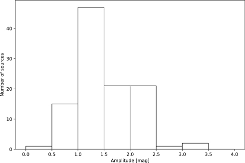
Figure 5. Amplitude histogram of Mira variables for which we determined their amplitude in this paper.
Download figure:
Standard image High-resolution image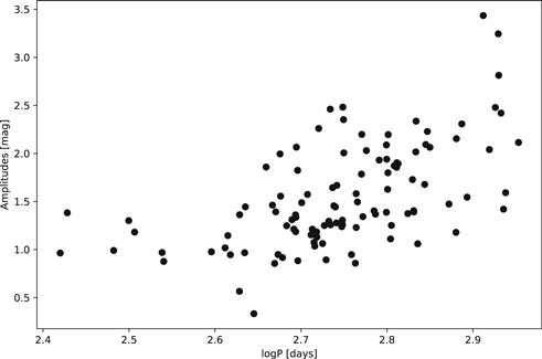
Figure 6. Period–amplitude diagram.
Download figure:
Standard image High-resolution image5. Distance Determination
5.1. Period–Luminosity Relation
The PLR of Mira variables was first established in the LMC and a recent evaluation of the PLR in the LMC was given in Ita & Matsunaga (2011). Since the PLR enables prediction of a star's absolute magnitude it is possible to calculate the distance modulus of Mira variables by combining measurements of the pulsation period and an extinction corrected apparent magnitude. We aim to estimate the distances of our long-period Mira variables using the PLR to reveal their distribution in our galaxy. The PLR of Mira variables at infrared wavelengths is a useful tool for distance determination within the Milky Way and at larger distances, since there is less extinction at these wavelengths.
The PLR at shorter wavelengths becomes imprecise for Mira variables with periods longer than about 300 days. C-rich Mira variables locate below the extension of the PLR along the period in the optical and JHKs bands (Ita & Matsunaga 2011). On the other hand, O-rich Mira variables with longer periods locate above the same extended PLR in the optical and JHKs bands. Some O-rich Mira variables with very long periods (log P > 3.0) are found below the extended PLR, probably due to circumstellar extinction, similarly to the C-rich Mira variables in the same paper. As a result of these deviations, the PLR at the K band or shorter wavelengths cannot be reliably used for the determination of distances. On the contrary, the 3.6 μm PLR in the same paper shows a tight and linear relation for both short and long-period members in the Spitzer 3.6 μm band, although it is based on single epoch data. This suggests that circumstellar extinction does not severely affect the PLR of longer period Mira variables at around 3 μm and thus can be used to more reliably determine distances.
In this paper, we combine the pulsation period of our monitoring observations we determined for the 108 long-period Mira variables with magnitudes from WISE (Wright et al. 2010) band I (3.4 μm) to estimate the distances to our sample via the 3.4 μm PLR. Our methodology is to first establish the 3.4 μm PLR. Second, we derive the interstellar extinction at 3.4 μm using a 3D reddening map. Finally, we derive the interstellar extinction corrected 3.4 μm magnitudes from the WISE data and use these to derive distance moduli for our sample.
In the present case, WISE is preferable to Spitzer since the latter does not contain data for all of our sources.
5.2. The PLR at 3.4 μm
To establish the PLR at 3.4 μm we use the photometries of 1663 Mira variables in the LMC, for which the periods were determined by OGLE-III (Soszyński et al. 2009). Since these sources are located in the LMC, we assume they reside equidistantly and the distance modulus of the LMC is 18.5. Figure 7 shows the apparent magnitudes of W1 from ALLWISE (Cutri et al. 2014) against their period for 1663 Mira variables listed in the OGLE-III catalog. We can see no significant difference in the distribution between C-rich and O-rich Mira variables. We performed least-square fitting to all sources regardless of C-rich and O-rich with a linear function. A least-square fitting to these data produces the following relation.


where MW1 is the absolute magnitude converted by the distance modulus of the LMC, and mW1 is the apparent magnitude in W1. Figure 8 is a histogram of the residual from the best-fit PLR. We use the width of the Gaussian, σ = 0.29 mag, as an error source in the following analysis. The 3.4 μm PLR is likely due to the balance of extinction and thermal radiation of circumstellar dust, and the two cases; Mira variables with and without the circumstellar dust, share the same position in the PL diagram.

Figure 7. 3.4 μm (W1) period–luminosity relation in the LMC. Gray points (cross) are O-rich Mira variables from the OGLE-III catalog. Black points (triangles) are C-rich Mira variables. Dotted line is the best-fit line of the least-square fitting for both O-rich and C-rich Mira variables.
Download figure:
Standard image High-resolution image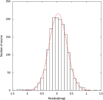
Figure 8. Histogram of the fitting of data points from the best-fit line. The red line shows the curve determined by applying a Gaussian filter.
Download figure:
Standard image High-resolution imageRiebel et al. (2010) also reported the 3.6 μm PLR of Mira variables in LMC using a similar data set, the MACHO (MAssive Compact Halo Objects survey) and the Spitzer SAGE catalog. They obtained the equations of PLR for the O-rich and C-rich Mira variables separately as well as for all sources including both the O-rich and C-rich Mira variables. The PLRs of O-rich and C-rich Mira variables give mW1 = 9.683 mag and 9.171 mag at log P = 2.7, and they differ from our relation (Equation (2)) by 0.123 mag and 0.389 mag, respectively. The PLR of all the sources replies mW1 = 9.156 mag at log P = 2.7 and their PLR differs from our relation (Equation (2)) by 0.138 mag. The difference for all the sources PLR is smaller than the residual of our fitting and is not significant considering the slight difference of wavelength (3.4 μm or 3.6 μm) and the difference of fitting range of period. In this paper, our purpose is to obtain distances for long-period Mira variables in Milky Way and so it is difficult to classify as O-rich or C-rich correctly for our samples and hence difficult to apply the PLR dedicated to the O-rich or C-rich Mira variables even if we know the equations of PLR for C-rich and O-rich separately. Therefore, we use our equation of PLR obtained from both C-rich and O-rich without discrimination in this paper.
5.3. Distance Modulus for Our Sources and Interstellar Extinction of Our Sample at 3.4 μm
We estimate distances to Mira variables using the 3.4 μm PLR. The apparent distance modulus at 3.4 μm is related to the true distance modulus μ and the extinction AW1 at 3.4 μm as follows.

Here, μ0 (=mW1 –MW1) is the apparent distance modulus without correction of interstellar extinction. Our sample, consisting of longer period Mira variables, resides in the Galactic plane. Thus, corrections must be derived for interstellar extinction at 3.4 μm as described below.
We determined AW1 using a 3D map of interstellar dust reddening, covering three-quarters of the sky (decl. > −25°) out to a distance of several kiloparsecs. (see http://argonaut.skymaps.info/; Green et al. 2018, 2015) They determined the interstellar reddening (E(B − V)) as a function of distance modulus for each line of sight using 800 million stars from Pan-STARRS 1 and 2MASS. Here, we use a universal dust extinction law with R(V) = 3.1 and  /E(B − V) = 0.157 to convert E(B − V) to AW1 (Schlafly & Finkbeiner 2011). On the other hand, interstellar extinction increases against distance modulus and AW1 is expressed as a monotonically increasing function (f(μ)) of μ. This function is provided as the "best-fit line" from the 3D reddening map. We can estimate the interstellar extinction and the distance modulus by solving the simultaneous equations of Equation (4) and f(μ). We show an example for IRAS 01304+6211 in the Figure 9. We used an error shown in the 3D reddening map. We summarize the AW1 values, the line-of-sight distances (D), and the height distances (z) in Table 1. We estimated the errors of μ using the error of PLR, the error of AW1 and the WISE photometric error.
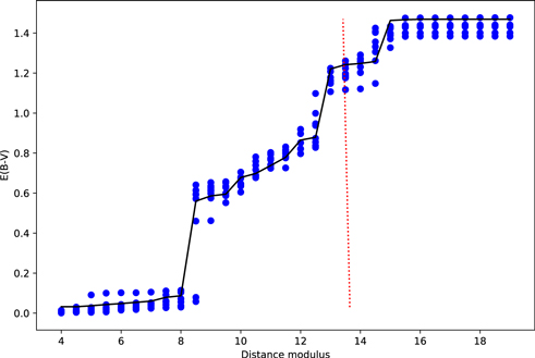
Figure 9. E(B − V) against the distance modulus based on the 3D reddening map for the direction toward IRAS 01304+6211. Blue points: E(B − V) from the 3D reddening map. Black line: the best-fit line of blue points provided by the 3D reddening map. Dotted red line: Equation (4) of IRAS 01304+6211.
Download figure:
Standard image High-resolution image6. Discussion
6.1. Face-on Distribution
Based on the distances derived from our monitoring survey we illustrate the Galactic face-on distribution of all of our Mira variables in Figure 10. To investigate the possibility that longer period Mira variables are associated with the spiral arm structures in the Milky Way, we compare our sample with the arm structure model derived from the distribution of HMSFRs (Reid et al. 2014). We will focus on the younger population, i.e., the subsample with 2.7 < log P < 3.0 and  < 300 pc, as shown in Figure 11.

Figure 10. Galactic face-on distribution of all Mira variables for which we determined their distance in this paper. The Galactic center is at (8, 0) and the Sun is at (0, 0).
Download figure:
Standard image High-resolution image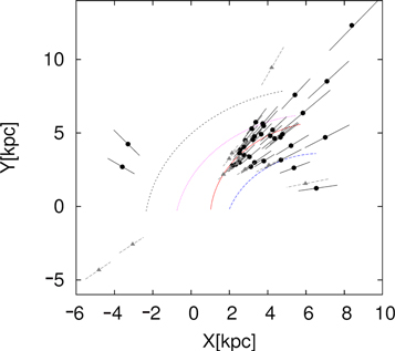
Figure 11. Galactic face-on distribution of our sample in the thin disk ( < 0.3 kpc). Black circle points: the sources located in
  < 0.3 kpc with the periods of log P > 2.7. Gray triangle points: the sources in
  < 0.3 kpc with the periods of log P < 2.7. The Galactic center is at (8, 0) and the Sun is at (0, 0). The distribution of HMSFR is sorted into individual arms which are represented by colors, Scutum arm, blue; Sagittarius arm, red; Local arm, violet; Perseus arm, black.
Download figure:
Standard image High-resolution imageThe distribution shows that longer period Mira variables are located near the Sagittarius arm (red line) and the Scutum arm (blue line). Figure 11 shows that our sample concentrates to 40° < l < 60°. This direction corresponds to the tangential direction of the Sagittarius arm and therefore the sources tend to be on the arm regardless of their distance. To investigate this effect, we examined the distance distribution of our sample in this direction. Figure 12 presents a histogram of the distances of sources located in 40° < l < 60° in Figure 11. There are 27 sources with 2.7 < log P < 3.0 in 40 < l < 60 and  < 300 pc, in which 23 sources (85%) are distributed in the range of 3 kpc and 8 kpc, corresponding to the Sagittarius arm. It is suggested to extend through 2 < D < 8 kpc in the 40° < l < 60° (Reid et al. 2014). Another two stars are located in the range of 9 < D < 12 kpc, corresponding to the Perseus arm (Reid et al. 2014). The more distant sample is likely to be incomplete because of the IRAS sensitivity limit.
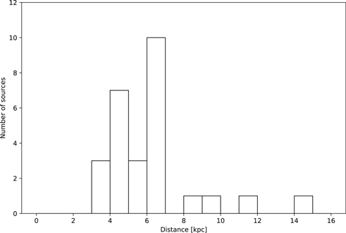
Figure 12. Histogram of the sources located in  < 300 pc and 40° < l < 60°.
Download figure:
Standard image High-resolution imageThe present result suggests that the distribution of longer period Mira variables probably trace the spiral arm structures of the Milky Way. In order to confirm our suggestion to the entire galaxy, it is necessary to search for more longer period Mira variables in other arms, for example, the Perseus arm and Outer arm.
6.2. Edge-on Distribution
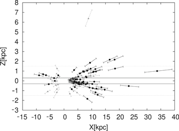
The edge-on distribution of our sample is shown in Figure 13. Approximately 50% of our sample is found to exist within the Galactic plane or  < 0.3 kpc, corresponding to the Galactic thin disk where metallicity is high, and star formation is active. We can see that the longer period Mira variables belonging to IIIa and IIIb regions in the IRAS two-color diagram are packed in the thin Galactic disk. Almost all the remaining 50% of sources are contained within the thick disk (
 < 1.5 kpc).
Figure 13. Edge-on distribution of our sample. Black points (circle) represent the sources with log P > 2.7. Gray points (triangle) represent the sources with log P < 2.7. The Galactic center is at (8, 0) and the Sun is at (0, 0). Black solid line:  = 0.3 kpc. Black dotted line:
  = 1.5 kpc.
Download figure:
Standard image High-resolution image
One source (IRAS 15106-1532) with a relatively shorter period (268 days) is found at 6.35 kpc from the Galactic plane. There are three possibilities of its high  position; (1) it was born at the Galactic plane and ejected outward, (2) born in the stream of local dwarf spheroidal galaxies (dsph) (Huxor & Grebel 2015), and (3) born in the halo of the Milky Way. In the case of (1), the stars born in the Galactic plane are randomized according to the rotation of the Milky Way over a long period of time. AGB stars like short-period Mira variables are widely distributed to the thick disk. However, it is difficult to explain IRAS 15106-1532 as having an origin in the galactic plane although it might just be an unexpected run-away star. It is necessary to create an accurate model of this moment; however, this will require taking into account the motion of stars or sudden phenomena such as blow-off from heavy stars in the Milky Way, so it is not possible to do this at the present moment. In the case of (2) stream or dsph, stars born in the dsph galaxies are pulled off by tidal force and a stream is formed. Some Mira variables are found both in the stream and in dsph galaxies (Mauron 2008; Sakamoto et al. 2012). However, the position of IRAS 15106-1532 does not match the distribution of the already known stream; therefore, IRAS 15106-1532 does not have a stream or dsph origin. In the case of (3), Whitelock (1990) reported that some Mira variables are born in a globular cluster in the halo, which are known to have short periods. It is possible to infer the origin of IRAS 15106-1532 in globular clusters in the halo.
We wish to thank the anonymous referee for a careful reading and useful comments on our manuscript. The Kagoshima University 1 m telescope is a member of the Optical and Near-infrared Astronomy Inter-University Cooperation Program and supported by it. This publication makes use of data products from the Two Micron All Sky Survey, which is a joint project of the University of Massachusetts and the Infrared Processing and Analysis Center/California Institute of Technology, funded by the National Aeronautics and Space Administration and the National Science Foundation. This publication makes use of data products from the Wide-field Infrared Survey Explorer, which is a joint project of the University of California, Los Angeles, and the Jet Propulsion Laboratory/California Institute of Technology, funded by the National Aeronautics and Space Administration. R.B. acknowledges support through the EACOA Fellowship from the East Asian Core Observatories Association.
Footnotes
- *
Released on 2019 October 4th.