


Abstract
Unlike ordinary supernovae (SNe), some of which are hydrogen and helium deficient (called Type Ic SNe), broad-lined Type Ic SNe (SNe Ic-bl) are very energetic events, and only SNe Ic-bl are coincident with long-duration gamma-ray bursts (GRBs). Understanding the progenitors of SN Ic-bl explosions versus those of their SN Ic cousins is key to understanding the SN–GRB relationship and jet production in massive stars. Here we present the largest existing set of host galaxy spectra of 28 SNe Ic and 14 SNe Ic-bl, all discovered by the same galaxy-untargeted survey, namely, the Palomar Transient Factory (PTF). We carefully measure their gas-phase metallicities, stellar masses (M*), and star formation rates (SFRs). We further reanalyze the hosts of 10 literature SN–GRBs using the same methods and compare them to our PTF SN hosts with the goal of constraining their progenitors from their local environments. We find that the metallicities, SFRs, and M* values of our PTF SN Ic-bl hosts are statistically comparable to those of SN–GRBs but significantly lower than those of the PTF SNe Ic. The mass–metallicity relations as defined by the SNe Ic-bl and SN–GRBs are not significantly different from the same relations as defined by Sloan Digital Sky Survey galaxies, contradicting claims by earlier works. Our findings point toward low metallicity as a crucial ingredient for SN Ic-bl and SN–GRB production since we are able to break the degeneracy between high SFR and low metallicity. We suggest that the PTF SNe Ic-bl may have produced jets that were choked inside the star or were able to break out of the star as unseen low-luminosity or off-axis GRBs.
Export citation and abstract BibTeX RIS
1. Introduction
Exploding massive stars in the form of supernovae (SNe) and long-duration gamma-ray bursts (LGRBs) are the most powerful explosions in the universe. They are visible over large cosmological distances, but uncovering their progenitors is a difficult task. The origin of LGRBs has been conclusively shown to be connected to the death of some kind of massive stars in the form of SNe (e.g., Galama et al. 1998; Hjorth et al. 2003; Stanek et al. 2003), also known as the SN–GRB connection, where the spectrum of all nearby bona fide LGRB afterglows metamorphosed into that of a Type Ic SN with broad lines (SN Ic-bl; e.g., Modjaz et al. 2006; for reviews, see Woosley & Janka 2005; Modjaz 2011; Cano et al. 2017b). SNe Ic are defined by the lack of H and He lines (for reviews, see Filippenko 1997; Gal-Yam 2016; Modjaz et al. 2019; and for a new way of classifying SNE Ic, see Williamson et al. 2019), indicating that the SN Ic progenitor has lost large amounts (if not all) of its H and He envelopes before explosion (Branch et al. 2006; Hachinger et al. 2012; Liu et al. 2016). In addition, a subclass of SNe Ic show broadened lines in their spectra (thus called SNe Ic-bl), indicating high ejecta expansion velocities of order 15,000–30,000 km s−1 (Modjaz et al. 2016; Sahu et al. 2018). Their kinetic energies are as high as ∼1052 erg s−1 according to some models (Mazzali et al. 2017), up to 10 times more than canonical SNe. While all bona fide LGRBs have been associated with SNe Ic-bl, there are many SNe Ic-bl without observed GRBs, and the big question is why.
Direct imaging of the progenitors of SNe Ic-bl with and without observed GRBs has thus far been unsuccessful (e.g., Gal-Yam et al. 2005; Eldridge et al. 2013), so the progenitors and the explosion conditions remain unclear and are the focus of current research. Although a better understanding of stellar evolution is an important goal in its own right, the question of SN and GRB progenitors impacts a diverse group of research fields. For instance, GRBs are suspected sites for high-energy cosmic-ray acceleration (Abbasi et al. 2012). GRBs and SNe are also a fundamental part of the chemical history of the universe, since particularly black-hole-forming SNe are thought to have made important contributions to the early chemical evolution of the universe (Nomoto et al. 2006). Finally, owing to their high luminosity, LGRBs can be detected at very high redshift. With the most distant GRB at redshift z ≈ 9.4 (Cucchiara et al. 2011), their mere existence at such distances makes them ideal tools to probe the star formation rate (SFR) history of the universe and provide constraints on the properties of interstellar dust, the reionization history, and star formation in the early universe (Wang & Dai 2011; Robertson & Ellis 2012; Perley et al. 2016a). The search for a unified model for GRBs and SNe Ic-bl is thus highly motivated.
SNe Ic-bl belong to the class of stripped-envelope core-collapse SNe (shortened to "stripped SNe"; Clocchiatti et al. 1997; Modjaz et al. 2014; Zapartas et al. 2017) and constitute a small fraction (∼4% of stripped SNe;18 Shivvers et al. 2017). Since the mechanism behind the energetic outflows in SNe Ic-bl is not clear, the role of GRBs in SNe Ic-bl is particularly interesting. Although not all SNe Ic-bl have been observed with an associated GRB (Berger et al. 2002; Soderberg et al. 2010; Margutti et al. 2014; Milisavljevic et al. 2015), all SNe associated with GRBs are of Type Ic-bl (for reviews, see, e.g., Woosley & Bloom 2006; Modjaz 2011; Cano et al. 2017b). In fact, for all bona fide LGRBs at z ⪅ 0.3 a corresponding SN Ic-bl has been found (e.g., Mazzali et al. 2014; Cano et al. 2017b).19 For the SNe Ic-bl accompanied by GRBs, GRB jets may be the reason for the broadened lines in SNe Ic-bl as shown by Barnes et al. (2018).
Several possible explanations as to why there are SNe Ic-bl without associated GRBs are as follows. Some of these will be qualitatively assessed in subsequent sections.
(1) The progenitor of the SN Ic-bl made a GRB, but it was off-axis. Off-axis GRBs are discussed further in Section 7.1.
(2) The broad lines in SNe Ic-bl have nothing to do with an engine, and no GRB is produced in association with those SNe Ic-bl that are seen without a GRB.
(3) An engine is present, but the jet did not punch through the stellar envelope, as it was too low in energy, was choked, or did not last sufficiently long (Margutti et al. 2014; Milisavljevic et al. 2015; Modjaz et al. 2016). Understanding which core-collapse SNe (CCSNe) harbor choked jets would also impact identifying the astrophysical sources for the diffuse flux of high-energy IceCube neutrinos (Senno et al. 2018).
If an engine is present, be it either a collapsar (Woosley et al. 1993; MacFadyen & Woosley 1999; MacFadyen et al. 2001) or a magnetar (Usov 1992; Thompson 1994; Wheeler et al. 2000; Thompson et al. 2004), one could suggest that jets occur in nearly all SNe Ic-bl, accelerating the outflows and causing line broadening, though GRBs are not always observed because they are either off-axis or stifled. We discuss this possibility later in the context of our results. In fact, recent observations by Soderberg et al. (2010), Margutti et al. (2014), and Chakraborti et al. (2015) show that there may be SN events that populate the gap between energetic but nonrelativistic SNe Ic-bl and SN–GRBs by producing relativistic, engine-driven outflows but no observable GRBs. With these new observations, the connection between SN–GRBs and SNe Ic-bl appears to become increasingly relevant.
Many studies have concluded that GRBs strongly prefer low-metallicity environments (e.g., Fynbo et al. 2003; Fruchter et al. 2006; Stanek et al. 2006; Modjaz et al. 2008a; Levesque et al. 2010a; Graham & Fruchter 2017). Furthermore, it is clear that LGRBs are linked to SNe Ic-bl, and their progenitors must be massive, rapidly rotating stars that have lost their H and He envelopes, with the ability to create significant quantities of Ni during the explosion (e.g., Mazzali et al. 2001; Maeda & Tominaga 2009; Cano et al. 2017b).
Several different mechanisms have been proposed to achieve the stripping of the stellar envelope, and from those mechanisms, single Wolf–Rayet (WR) stars and binary star systems emerge as GRB/SN Ic-bl progenitor channels (for recent reviews, see, e.g., Smartt 2015; Levan et al. 2016). Binary star systems and WR channels can also be at play at the same time: for instance, Cantiello et al. (2007) suggest that LGRB progenitors can be made through quasi-chemically homogeneous evolution in low-metallicity environments once a WR star has been spun up in a massive close binary.
Since massive stars and binary star systems are likely progenitor channels for stripped CCSNe, such as SNe Ic-bl that are linked to GRBs, it is interesting to look for environmental markers that favor the evolution of such channels. Aside from envelope stripping, binary systems provide mechanisms of retaining or gaining angular momentum, which is important for GRB progenitor models. Stars in binary systems may be spun up by the accretion of material, direct mergers, or tidal locking in tight binaries (e.g., Cantiello et al. 2007). Kelly et al. (2014) found that hosts of SNe Ic-bl and GRBs in their sample have high SFR and mass densities, after carefully correcting for systematics, and suggested that binary interaction rates may be higher in those environments. Wang & Dai (2011) show that variations in the stellar initial mass function (IMF) such as those proposed by Davé (2008) could lead to higher rates of close-binary systems or more massive stars in galaxies, both of which are associated with the occurrence of GRBs. If GRBs were products of dynamical processes in young dense star clusters as suggested by van den Heuvel & Portegies Zwart (2013), GRBs would clearly prefer host galaxies with the highest SFRs.
Although multiple studies have shown that GRBs prefer low-metallicity environments (see above), it is still somewhat debated whether low metallicity causes GRB progenitors to form, or whether it is a side effect of high specific SFR (sSFR; SFR per unit mass), since there is a galaxy relationship in which high sSFR galaxies are also metal-poor (e.g., Mannucci et al. 2011). Here we compare the sSFR of the host galaxies of Palomar Transient Factory (PTF; Law et al. 2009) stripped SNe with those of SN–GRBs (something not done before), as well as with those of the general population of star-forming galaxies, to test whether the hosts of SNe Ic-bl without GRBs, as well as those of PTF SNe Ic, are as highly star-forming as GRB hosts, and to conclusively test whether low metallicity is the necessary ingredient for producing jets.
Until recently, GRBs and SNe were typically detected in different ways. GRBs are found in all-sky surveys with gamma-ray satellites such as BATSE, HETE, or Swift, and there is little or no host galaxy bias associated with their detection. However, traditional SN searches such as the Lick Observatory Supernova Search (LOSS; Filippenko et al. 2001) or CHASE (Pignata et al. 2009), with their small fields of view, specifically target luminous galaxies that contain many stars, in order to increase their odds of finding those that explode as SNe. Because more luminous galaxies are more metal-rich (Tremonti et al. 2004), including SNe that were found by targeted surveys introduces a bias toward finding SNe in high-metallicity regions (Modjaz et al. 2008a; Young et al. 2008; Sanders et al. 2012), complicating the comparison of the environments of the two kinds of stellar explosions. While Modjaz et al. (2008a), for the first time, pointed out that the targeted surveys are biased toward galaxies that are massive and thus more metal-rich, they could only include half of their SN Ic-bl sample from untargeted surveys, given the limited number of such surveys at that time. Thus, a large sample of SNe from an untargeted survey has to be examined to truly compare the environments of SNe with and without GRBs.
Here we fulfill this requirement by exploiting the largest single-survey, untargeted, spectroscopically classified, and homogeneous collection of SNe Ic and SNe Ic-bl discovered by the PTF before 2013 and by conducting an unparalleled and thorough study of their host galaxies. PTF alleviates the aforementioned galaxy bias (and thus the implied metallicity bias), since the 1.2 m telescope at Palomar Observatory observes a much larger patch of the sky with its 7.2 deg2 field of view (Law et al. 2009; Rau et al. 2009). On top of omitting bias, our sample with directly measured metallicities provides a factor of ∼2 increase in SNe Ic and SNe Ic-bl from untargeted surveys compared to previous studies (Modjaz et al. 2008a; Arcavi et al. 2010; Kelly & Kirshner 2012; Sanders et al. 2012) and a factor of 1.5–2 increase for the SN–GRB hosts compared to other SN–GRB host compilation studies (e.g., Modjaz et al. 2008a; Levesque et al. 2010a).
We study the environments of a large sample of members of the SN Ic family, namely, SNe Ic and SNe Ic-bl, in order to discern systematic trends that characterize their stellar populations. In order to pinpoint the physical processes that give rise to observed jets during the explosions of some massive stripped stars in the form of GRBs, we compare them to host galaxies of SN–GRBs (that is, SNe Ic-bl with an associated GRB) in order to uncover any differences in the host galaxies and environments of SNe Ic-bl with and without observed GRBs. Thus, we compare derived galaxy properties such as metallicity and SFR with those of published host galaxies of 10 SN–GRBs with spectroscopic classifications at z ⪅ 0.3, whose emission-line intensities we take from the literature and analyze in the same way as our SN Ic-bl hosts in order to ensure a self-consistent comparison. We also report the uncertainty estimates for the SN–GRB host galaxy parameters that we measure from the literature spectra, which previous studies did not report (see, e.g., Levesque et al. 2010a).
Levesque et al. (2010b) suggested that SN–GRBs prefer special kinds of galaxies that follow a different mass–metallicity relationship than a comparison sample of Sloan Digital Sky Survey (SDSS) galaxies, namely, ones that exhibit lower metallicities for the same galaxy masses. However, the available host data set of SN–GRBs was relatively small in 2010 (only five objects). In the subsequent eight years, five more SN–GRBs have been discovered, doubling the initial sample. We include the most recent SN–GRBs in our study, and we revisit the question whether SN–GRBs prefer a special population of galaxies. In addition, progress has been made in the field of measuring chemical abundances, and thus we are including new metallicity scales in our work here.
In Section 2, we introduce the PTF SNe in our sample. Section 3 gives details of the spectroscopic and photometric data of the PTF SN host galaxies. We introduce a sample of GRBs in Section 4, and we describe how we derived host galaxy properties from the literature for comparison with our PTF SN host galaxies. In Section 5, we explain how the SN host galaxy properties were derived, including the metallicities for the entire sample and M* values and SFRs for PTF SNe Ic/Ic-bl host galaxies only. Sections 6 and 7 present our results and discuss implications for jet production and GRB progenitor models. Potential caveats in our work are described in Section 8, and Section 9 summarizes our conclusions. Throughout the paper, we adopt a Hubble constant of H0 = 70 km s−1 Mpc−1.
2. Discovery of PTF SNe Ic and SNe Ic-bl
Our study is based on the SN harvest of the PTF survey between 2009 and 2012, a galaxy-untargeted and wide-field (7.2 deg2 field of view) search, discovering transients up to a limiting magnitude of 20.5 in the Mould R band, independent of their host galaxies. While here we concentrate specifically on PTF SNe Ic and SNe Ic-bl, more details about the discovery and analysis of PTF SNe Ib/c are given by Corsi et al. (2016), Fremling et al. (2018), Taddia et al. (2019), and C. Barbarino et al. (2019, in preparation). Independent of Fremling et al. (2018), we performed our own spectral classification on the PTF SN spectra by running the state-of-the-art code SNID (Blondin & Tonry 2007), with the augmented SNID library of stripped SNe and superluminous SNe Ic published by the SNYU group (Liu & Modjaz 2014; Liu et al. 2016, 2017; Modjaz et al. 2016). Our spectroscopic identifications (IDs) are given in Table 1. For a number of PTF SNe, we have updated their spectroscopic IDs, while they had been announced or published with a different ID.20 We note that while our IDs for the PTF SNe Ic-bl in our sample are fully consistent with those of Corsi et al. (2016), some of our IDs are inconsistent with those of Fremling et al. (2018) (F18); in particular, PTF10tqv and PTF11qcj are included as SNe Ic-bl in our sample, but F18 include them as SNe Ic, and all the SNe in our "uncertain ID" group, except PTF10gvb, are included as SNe Ic by F18.
Table 1. SN Host Galaxy Sample and Spectroscopy
| PTF | z | UT Date | Tel. | Instr. | Res. (r/b) | P.A. | Airmass | Seeing (r/b) | Slit | Exp. (r/b |
|---|---|---|---|---|---|---|---|---|---|---|
| Name | (Å) | (deg) | (arcsec) | (arcsec) | if Different) (s) | |||||
| SN Ic-bl | ||||||||||
| 09sk | 0.035 | 2016 Feb 9 | Keck | LRIS | 6.6/4.6 | 360.00 | 1.03 | 1.0/1.1 | 1.0 | 900/980 |
| 10aavz | 0.062 | 2014 Nov 21 | Keck | LRIS | 9.3/5.9 | 34.40 | 1.56 | 1.9/1.7 | 1.5 | 1200 × 2 + 900 |
| 10bzfa | 0.049 | 2016 Jun 06 | Keck | LRIS | 6.4/4.3 | 4.01 | 1.35 | 1.3/1.3 | 1.0 | 600 × 2/620 + 640 |
| 10ciw | 0.115 | 2015 Jun 15 | Keck | LRIS | 6.2/4.7 | 48.00 | 1.07 | 0.93/1.0 | 1.0 | 900 × 3 |
| 10qts | 0.09 | 2015 Jun 15 | Keck | LRIS | 6.2/4.7 | 35.00 | 1.10 | 0.93/1.0 | 1.0 | 1200 × 3 |
| 10tqv | 0.079 | 2016 Jun 10 | Keck | LRIS | 6.2/7.8 | 59.00 | 1.38 | 0.94/1.0 | 1.0 | 1200 × 2/1200 |
| 10vgv | 0.015 | 2015 Jun 15 | Keck | LRIS | 6.2/4.7 | 236.00 | 1.21 | 0.93/1.0 | 1.0 | 900 × 2 |
| 10xem | 0.056 | 2014 Nov 21 | Keck | LRIS | 6.1/4.8 | 256.60 | 1.02 | 0.86/1.1 | 1.0 | 900 × 2 |
| 11cmh | 0.1055 | 2016 Jun 06 | Keck | LRIS | 6.4/4.3 | 73.70 | 1.72 | 1.3/1.3 | 1.0 | 1000 × 2/1040 × 2 |
| 11gcj | 0.148 | 2017 Jun 25 | Keck | LRIS | 6.3/4.6 | 80.00 | 2.10 | 0.84/0.89 | 1.0 | 900 × 2/900 + 1020 |
| 11img | 0.158 | 2016 Sep 9 | Keck | LRIS | 6.1/4.5 | 211.00 | 1.39 | 1.1/1.2 | 1.0 | 1200 × 2/1200 + 1340 |
| 11lbm | 0.039 | 2014 Nov 21 | Keck | LRIS | 6.1/4.8 | 98.49 | 1.17 | 0.86/1.1 | 1.0 | 1200 |
| 11qcj | 0.028 | 2011 Dec 31 | Keck | LRIS | 6.4/8.8 | 245.00 | 1.36 | 1.0/0.94 | 1.0 | 420 × 2/900 |
| 12as | 0.033 | 2012 Apr 27 | Keck | LRIS | 5.3/6.5 | 30.00 | 1.07 | 1.0/0.96 | 0.7 | 540 × 2/1200 |
| SN Ic | ||||||||||
| 09iqd | 0.034 | 2010 Jan 9 | Keck | LRIS | 4.6/3.7 | 141.00 | 1.11 | 0.81/0.95 | 1.0 | 150 × 2/420 |
| 10bhu | 0.036 | 2015 Jun 13 | P200 | DBSP | 5.3/3.8 | 153.00 | 1.09 | 1.3/1.6 | 1.0 | 900 × 3 |
| 10fmx | 0.045 | 2015 Jun 13 | P200 | DBSP | 5.3/3.8 | 227.00 | 1.07 | 1.3/1.6 | 1.0 | 900 × 3 |
| 10hfe | 0.049 | 2010 Jun 8 | Keck | LRIS | 6.5/8.2 | 127.00 | 1.71 | 0.80/0.93 | 1.0 | 260 × 2/600 |
| 10hie | 0.067 | 2015 Jun 13 | P200 | DBSP | 6.8/4.2 | 265.00 | 1.13 | 1.3/1.6 | 1.5 | 900 × 2 |
| 10lbo | 0.053 | 2016 Feb 9 | Keck | LRIS | 6.6/4.6 | 289.60 | 1.33 | 1.0/1.1 | 1.0 | 600/680 |
| 10ood | 0.059 | 2010 Sep 5 | Keck | LRIS | 5.2/5.2 | 226.00 | 1.13 | 0.68/0.71 | 0.7 | 150 × 2/420 |
| 10osn | 0.038 | 2014 Sep 30 | P200 | DBSP | 3.6/4.5 | 101.51 | 1.04 | 1.3/1.7 | 1.5 | 900 × 2 |
| 10qqd | 0.08 | 2015 Jun 13 | P200 | DBSP | 6.8/4.2 | 201.00 | 1.14 | 1.3/1.6 | 1.5 | 900 |
| 10tqi | 0.038 | 2014 Nov 21 | Keck | LRIS | 6.1/4.8 | 262.74 | 1.16 | 0.86/1.1 | 1.0 | 1200 |
| 10wal | 0.028 | 2014 Nov 21 | Keck | LRIS | 6.1/4.8 | 214.60 | 1.22 | 0.86/1.1 | 1.0 | 1200 × 2 + 300/1200 × 2 |
| 10xik | 0.071 | 2014 Nov 21 | Keck | LRIS | 6.1/4.8 | 231.10 | 1.28 | 0.86/1.1 | 1.0 | 1200 × 2 |
| 10yow | 0.024 | 2015 Jun 13 | P200 | DBSP | 6.8/4.2 | 321.01 | 1.16 | 1.3/1.6 | 1.5 | 900 × 3 |
| 10ysdb | 0.096 | 2014 Sep 30 | P200 | DBSP | 3.6/4.5 | 351.90 | 1.04 | 1.3/1.7 | 1.5 | 900 × 2 |
| 10zcn | 0.02 | 2014 Sep 30 | P200 | DBSP | 3.6/4.5 | 177.41 | 1.01 | 1.3/1.7 | 1.5 | 900 × 2 |
| 11bovc | 0.022 | 2012 Jan 18 | P200 | DBSP | 6.4/4.4 | 330.01 | 1.03 | 1.9/2.4 | 1.5 | 600/1200 |
| 11hygd | 0.03 | 2014 Sep 30 | P200 | DBSP | 3.6/4.5 | 123.61 | 1.12 | 1.3/1.7 | 1.5 | 900 × 2 |
| 11ixk | 0.021 | 2015 Jun 12 | P200 | DBSP | 5.2/3.6 | 206.01 | 1.06 | 1.1/1.5 | 1.0 | 900 × 2 |
| 11jgj | 0.04 | 2015 Jun 13 | P200 | DBSP | 6.8/4.2 | 74.60 | 1.17 | 1.3/1.6 | 1.5 | 900 × 2 |
| 11klg | 0.026 | 2014 Nov 21 | Keck | LRIS | 6.1/4.8 | 274.79 | 1.03 | 0.86/1.1 | 1.0 | 1200 |
| 11rka | 0.074 | 2015 Jun 15 | Keck | LRIS | 6.2/4.7 | 55.00 | 1.04 | 0.93/1.0 | 1.0 | 900 |
| 12cjy | 0.044 | 2015 Jun 12 | P200 | DBSP | 6.6/4.3 | 290.00 | 1.07 | 1.1/1.5 | 1.5 | 900 × 2 |
| 12dcp | 0.031 | 2012 May 17 | Keck | LRIS | 1.9/3.6 | 231.00 | 1.05 | 0.94/0.92 | 1.0 | 600 |
| 12dtf | 0.061 | 2014 Sep 30 | P200 | DBSP | 3.6/4.5 | 95.00 | 1.15 | 1.3/1.7 | 1.5 | 900 × 2 |
| 12fgw | 0.055 | 2015 Jun 12 | P200 | DBSP | 6.6/4.3 | 297.01 | 1.00 | 1.1/1.5 | 1.5 | 900 × 2 |
| 12jxd | 0.025 | 2014 Nov 21 | Keck | LRIS | 9.3/5.9 | 357.85 | 1.13 | 1.9/1.7 | 1.5 | 1200 |
| 12ktu | 0.031 | 2014 Sep 30 | P200 | DBSP | 3.6/4.5 | 7.90 | 1.38 | 1.3/1.7 | 1.5 | 900 × 2 |
| Weird/Uncertain SN Subtype | ||||||||||
| 09pse | 0.106 | 2015 Jun 13 | P200 | DBSP | 6.8/4.2 | 141.00 | 1.10 | 1.3/1.6 | 1.5 | 900 × 2 |
| 10bipe | 0.051 | 2011 Jun 30 | Gemini-S | GMOS-S | 7.7 | 155.6 | 1.57 | 0.7 | 1.0 | 1200 |
| 10gvbf | 0.1 | 2015 Apr 23 | Keck | LRIS | 6.1/6.6 | 270.00 | 1.07 | 1.1/1.3 | 1.0 | 500 + 580/600 × 2 |
| 10svtg | 0.031 | 2014 Nov 21 | Keck | LRIS | 9.3/5.9 | 168.11 | 1.62 | 1.9/1.7 | 1.5 | 1200 |
| 12hnif | 0.107 | 2016 Oct 25 | Keck | DEIMOS | 5 | 116.0 | 1.31 | 0.6 | 1.2 | 600 × 2 |
Notes.
aAlso known as SN 2010ah. bAlso known as SN 2011bm. cAlso known as SN 2011ee. dSN 2004aw-like, thus possibly a transition object between SN Ic and SN Ic-bl. eSN Ic/Ic-bl. fSLSN/SN Ic-bl; Quimby et al. (2018) independently ID it as a possible SLSN Ic with Superfit, a different SN classification code. gSN Ib/c.Download table as: ASCIITypeset image
Although our sample consists of 14 SNe Ic-bl and 28 SNe Ic, we also include the host galaxy data of five SNe with uncertain or peculiar SN types—those were cases where the classification was not clear based on either low signal-to-noise-ratio (S/N) spectra or their uncertain physical nature. In particular, we have two SNe, PTF10gvb and PTF12hni, whose spectra match with those of both SNe Ic-bl and SLSNe Ic, since the spectra of SLSNe Ic contain broad lines, similar to those of SNe Ic-bl (Liu et al. 2017; Quimby et al. 2018)—and indeed Quimby et al. (2018) independently classify them as possible SLSNe Ic based on their own code. However, for our final analysis and statistical tests on the host galaxy data, we only include SNe Ic-bl and SNe Ic with clean IDs.
While the final PTF sample includes two additional SNe Ic with clean IDs for which we were not able to obtain host galaxy spectra (PTF09dh and PTF11mnb; for the latter see Taddia et al. 2017 for its peculiar spectra and spectral ID), we are confident that their omission will not affect our results; all of our conclusions are limited by the small number statistics of PTF SNe Ic-bl and the comparison sample of SN–GRBs, not those of PTF SNe Ic.
3. PTF SN Host Data
In this section, we describe data of the PTF SN host galaxies. We give details on how we conduct the spectroscopic observations, reduce and extract spectra, and measure emission-line fluxes from the spectra, as well as on how we query the SDSS archive for emission-line fluxes. We also explain how we assemble reliable ultraviolet (UV) to optical broadband photometry from SDSS, Pan-STARRS, and the Galaxy Evolution Explorer (GALEX). At the end of the section, we briefly discuss the redshift and luminosity distributions of the full sample, and we point out unique aspects of our sample. We also check that there are no obvious biases introduced when comparing the different SN host galaxies in our sample.
Host galaxy spectra of a total of seven PTF SNe Ic and SNe Ic-bl in our sample have been obtained and published independently by Sanders et al. (2012). We compare our data and analysis with theirs in detail in Appendix D. Overall, their metallicity values agree with ours (except for PTF11hyg); however, we have better data, possess the most updated spectroscopic IDs for the PTF SNe, and analyze the data with more recent metallicity scales.
3.1. Spectroscopic Data
3.1.1. Spectroscopic Observations and Reduction
Optical spectra were obtained with a variety of telescopes: the 10 m Keck I and Keck II telescopes, the 200-inch (5 m) Hale telescope of Palomar Observatory (P200), and the 8.1 m Gemini-North and Gemini-South telescopes. The spectrographs employed were the Low Resolution Imaging Spectrometer (LRIS; Oke et al. 1995) at Keck I and DEIMOS (Faber et al. 2003) at Keck II, the Double Spectrograph (DBSP; Oke & Gunn 1982) on the P200, and the GMOS-North and GMOS-South (Hook et al. 2003) at Gemini.
The majority of our host galaxy spectra were obtained long after the SNe themselves had faded, including the Keck and P200 runs after 2013 and Gemini runs during 2011. We expect such host spectra to have minimum contamination from the SN emission. Exposure times were chosen to yield S/N > 15 in the Hα line, in order to robustly determine the line flux ratios for metallicity diagnostics. We reobserved if the desired S/N was not reached in an earlier run, but only the spectrum of the best quality for a given host is presented in this paper.
During our major observing runs with Keck I, the spectra of nine hosts were obtained on 2014 November 21 (UT dates are used throughout this paper) and of four hosts on 2015 June 15. We used a 600/4000 grism on the blue side and a 400/8500 grating on the red side, yielding an FWHM resolution of ∼4 Å and ∼7 Å on the blue and red sides (respectively) with a slit width of 1''. The spectrograph and dichroic setup allows continuous wavelength coverage of at least 3500–8000 Å. Given the redshifts of our targets, all of the major nebular emission lines required to derive oxygen abundances, including [O ii] λλ3726, 3729, are within this wavelength range. We used Hg–Ne–Ar comparison lamps for the wavelength calibration. Standard bias frames and lamp flats were obtained for each night. Several standard stars were taken during the nights for the flux calibration.
We placed the slit center at the SN site to catch the immediate environment of the explosion, which can be significantly different from the galaxy nucleus owing to metallicity gradients. LRIS is equipped with an atmospheric dispersion corrector, which allowed us to orient the slit at an angle different from parallactic angle (Filippenko 1982) without any loss from atmospheric dispersion. We chose a position angle (P.A.) that covered both the SN position and the nucleus of the host galaxy along the radial direction. If the SN site is far away from the nucleus with little local host galaxy emission, we can still characterize host properties via the brighter regions closer to the nucleus that fall within our slit. In fact, this only happens for a few cases among the full sample, and they are distinguished by different symbols on the plots in our analysis. A slit width of either 1 0 or 15 was used, depending on the seeing conditions.
In addition, nine host spectra presented here were acquired at Keck in 2015–2017 (one with DEIMOS and all others with LRIS), with similar instrumental setups to our major Keck runs in 2014 and 2015, so as to deliver a homogeneous data set. Note that the wavelength coverage of the DEIMOS observation starts at 4500 Å; thus, the [O ii] λλ3726, 3729 doublet is outside our coverage for the host galaxy of PTF12hni.
The P200 runs were conducted on 2014 September 30 (for six hosts) and 2015 June 12 and 13 (for 10 hosts), following similar conventions to the Keck runs (e.g., the SN sites were placed at the slit center). We took Fe–Ar comparison-lamp exposures on the blue side and He–Ne–Ar on the red side. The brighter hosts were preferentially observed during the P200 runs.
One host spectrum presented here (of PTF10bip) was obtained with Gemini-South, and the [O ii] λλ3726, 3729 doublet lies outside of the wavelength coverage.
In addition, we gathered data for hosts of five PTF SNe Ic and two PTF SNe Ic-bl that were observed in the year 2012 or earlier when the SN was still present (one of them with P200 and the rest with Keck I; the SN Ic spectra have been published by Fremling et al. 2018). Thus, we can easily locate the SN sites by the bright continuum of SN light in the two-dimensional frames. While the SN spectra were superimposed on the spectra of their host galaxies, we were able to remove them during the analysis since SN spectra have much broader lines than the H ii regions (see Section 3.1.3).
Details about our spectroscopic observations for 46 host galaxies of the PTF SNe in our sample (not including two, PTF12gzk and PTF12hvv, for which we downloaded SDSS spectra; see Section 3.1.4) are shown in Table 1, including both the ones from our recent runs and earlier ones based on data with SN spectra superimposed. Column (1) lists the name of the PTF SN, with the first two digits being the year of SN detection. Column (2) indicates the most up-to-date SN classification performed by us. Column (3) lists the UT date of the observations. The ones based on data with SN spectra superimposed have a UT date in the year 2012 or earlier. Columns (4) and (5) list the telescope and instrument used: Keck I (LRIS), Keck II (DEIMOS), Gemini-S (GMOS-S), or P200 (DBSP). Column (6) lists the spectral resolution on the red and blue sides, respectively. They were measured from the width of night-sky lines, or of comparison-lamp lines if only a few night-sky lines exist on the blue-side spectra. Column (7) lists the position angle of the slit in degrees east of north, Column (8) the airmass, Column (9) the seeing, and Column (10) the slit width. In Column (11) we give the exposure time, with the red and blue sides separated by a slash in case they differ. All but 2 spectra have a minimum wavelength range of 3,300 Å to 8,200 Å. The two spectra that do not, have a range of 4500-9600 Å (DEIMOS) and of 4000-7200 Å (GMOS-S).
3.1.2. Spectroscopic Reduction and Analysis
We followed standard procedures in IRAF to prepare the Keck/LRIS data obtained from our major runs in 2014 and 2015 for further reduction, including bias subtraction, trimming, and flat-fielding. For the LRIS data obtained before 2013, as well as in 2015–2017 following our major runs, the preprocessing was performed by the automated reduction pipeline in IDL, LPipe (Perley 2019), which delivers similar results to the standard procedures in IRAF. For the P200/DBSP data, we preprocessed with a PyRAF-based reduction pipeline, pyraf-dbsp (Bellm & Sesar 2016).
Subsequent cosmic-ray removal, spectrum extraction, and wavelength calibration were performed in the same manner for all data sets. If at least three exposures were taken on the same target, the imcombine task was performed in IRAF using median-image combine to remove cosmic rays. Otherwise, we ran the IDL routine P-Zap21 for cosmic-ray removal, which has been improved for better treatment around bright emission-line regions and absorption features in standard-star spectra. We adopted optimal spectrum extraction from the IRAF task, apall, which by nature applies higher weights to brighter regions in the aperture. The metallicity measurement as a result can be considered as a luminosity-weighted average over the aperture. The final steps of flux calibration, atmospheric band removal, and refinement of wavelength calibration against night-sky lines were performed by our customized IDL routines (Matheson et al. 2001).
In particular, we carefully select apertures for spectrum extraction to best probe the immediate environments of SNe. The spectra should also provide sufficient S/N in major nebular emission lines for metallicity calculation. As a result, we center the aperture at the peak of Hα emission from the nearest star-forming region to the SN site in the slit. However, we caution that we use the term star-forming region here to infer a cluster of regions with significant Hα emission. We cannot spatially resolve individual star-forming regions given the distances of our sources. Given that the progenitors of SNe Ic/Ic-bl are likely to be massive stars with a short lifetime, they generally have not traveled far away from the star-forming regions since birth until explosion. We confirmed by our data that star-forming regions with plenty of Hα emission are usually found very close to the SN site, with an offset usually comparable to the seeing.
Observed long after explosion, most SNe themselves were no longer visible in our data. During our observations, we located the SN site by offsetting from a nearby bright star in the finder chart that was obtained when the SN was still present. In order to locate the SN site along the slit during spectrum extraction, we placed the SN site at the slit center, as well as took standard-star exposures at the slit center. The positional accuracy of the SN site in the slit is comparable to the seeing as determined in this way by matching to the position of standard stars. We therefore chose an aperture size for spectrum extraction to be twice the seeing. Together with the fact that the aperture is centered at the nearest star-forming region, which is usually very nearby, this ensures that the SN site falls within the aperture for most of our targets. We denote such apertures as the SN sites in the subsequent analysis. In the remaining small number of cases (7 out of all 46 host spectra that we extracted), the SN sites have large offsets from the host nucleus or simply are in regions with little Hα emission; for them, the above strategy of aperture placement leaves the SN site outside the aperture. We denote such apertures as "Hii" instead, or "nuc" if that peak of Hα emission also happens to be at the galaxy nucleus. In order to extract spectra with emission lines detected, we compromised by using a region farther away from the SN site in such cases. They are less representative of the immediate environments of the SN explosions and are plotted with different symbols in the figures. However, they constitute only a small fraction (7/48) of all the host spectra that we extracted.
It is also important to appropriately select sky background regions during spectrum extraction. For most projects aimed at the study of SNe themselves as point sources, background regions closely bracketing the SN sites in the slit are chosen. However, the emission from the host galaxy is extended, so that such close backgrounds may still contain star-forming regions from other parts within the same galaxy. Considering that the nebular emission-line ratios vary throughout the galaxy, choosing close background regions would effectively alter the line flux ratios arising from the star-forming region near the SN site from their intrinsic values. We instead chose to place the background regions sufficiently far out to avoid the extended emission from host galaxies, such that they only contain night sky, not galaxy light. Because the background regions are far away from the SN site in extended galaxies, the host spectra extracted at the SN site can be very noisy at the wavelengths of night-sky lines. Such artifacts are masked out during line flux measurements but lead to high uncertainty in the line flux value if that nebular emission line coincides with a night-sky line.
Our final host spectra are released both on the github page of our SNYU group22 and on WISEREP23 (Yaron & Gal-Yam 2012). Figures 1 and 2 show examples of our spectra for SNe Ic-bl and SNe Ic hosts, respectively, that represent both high-S/N and low-S/N cases, with our spectral fits (which we describe in the next section) superimposed.

Figure 1. Two examples of the host galaxy spectra of SNe Ic-bl in our sample with spectral fits superimposed: the top panel shows a high-S/N spectrum (PTF09ks host, taken of the nucleus), while the bottom panel shows an example of a low-S/N spectrum (PTF10aavz host, taken at the SN site) among the host spectra in our sample. The spectral fits, shown in different colors, are the outputs of platefit, the standard spectral fitting pipeline for SDSS (Brinchmann et al. 2004; Tremonti et al. 2004), decomposing the original spectrum into three components: a continuum (blue), an emission-line spectrum (green), and the sum of continuum, nebular fit, and residuals shown in orange; see Section 3.1.3 for more details. On the right are close-up views of a few of the important lines used for reddening correction and metallicity measurements. Note the importance of stellar absorption removal necessary for obtaining correct Balmer emission-line intensities that are used for the subsequent analysis.
Download figure:
Standard image High-resolution image
Figure 2. Same as in Figure 1, but for two example hosts of PTF SNe Ic in our sample.
Download figure:
Standard image High-resolution image3.1.3. Line Flux Measurements
In this paper we focus on the analysis of the nebular emission lines of the host galaxy, since they encode physically important properties of the star-forming regions at the SN sites. However, the presence of stellar absorption features can contaminate the emission components, especially the Balmer lines (e.g., Tremonti et al. 2004). For both the Keck/LRIS and P200/DBSP data, in order to subtract stellar spectra and measure line fluxes from pure nebular emission spectra, we employed the SDSS standard spectral fitting pipeline, platefit (Brinchmann et al. 2004; Tremonti et al. 2004), which can be applied to non-SDSS data. Stellar absorption is usually non-negligible, especially in Hβ and Hγ, even for the spectra extracted at the SN sites that are offset from the galaxy nuclei, as shown in the example host spectra (Figures 1 and 2).
The platefit pipeline models the observed spectrum as a combination of three components: stellar continuum, nebular emission lines, and residual, as also shown in the example plots. The continuum, including all stellar absorption features, is fit to the observed spectrum with the emission-line features masked, using stellar population synthesis templates from Bruzual & Charlot (2003). This approach ensures better constraints on the amounts of stellar absorption than on those derived by only fitting to the wings of absorption features for one Balmer line at a time. The redshift of emission lines is not tied to that of the continuum; it is determined by the fit of a sum of Gaussian functions to the emission-line-only spectrum, assuming that the emission lines have the same velocity offset. Visual inspection confirms that the final fit can very well reproduce the observed spectra, including the wings of the Balmer lines and the global slope of the continuum, with the residuals only being significant at the edges of spectra with unphysical trends, or if there are SN features superimposed on the host spectra (see below).
The full spectra were separated into blue and red sides for both the Keck/LRIS and P200/DBSP data. We stitched the two spectra by applying a scaling factor on the blue side to match the continuum level over the overlapping wavelength regions on both sides. Since the transmission drops off rapidly at the edges of both spectra, small deviations in the wavelength calibration convert to large ones in the flux calibration. Unrealistic rising or falling trends at the edges make it hard to stitch by matching the observed continuum, whereas platefit's residual component characterizes such nonphysical trends. To stitch the blue-side and red-side spectra together, we match the continuum fit as an output component from platefit, free of the artificial rising or falling trends (included in the residual component). We therefore ran platefit twice: the first time to obtain the continuum fits for the two sides in order to then stitch them, and the second time on the stitched spectrum in order to obtain the spectrum with pure nebular emission lines that we use for line flux measurements. The line flux measurements that we present in Appendix A are based on standard single-Gaussian fits to the pure nebular emission-line spectrum and are corrected for Galactic reddening.
To ensure that the automated pipeline, platefit, is working properly on our spectra, we compare the line flux measurements given by platefit with the values we measured by hand via the splot task in IRAF. The platefit method derives uncertainties in line fluxes by the Levenberg–Marquardt least-squares fitting, and we follow Pérez-Montero & Díaz (2003) to derive statistical errors on the splot line fluxes. The uncertainty in the scaling factor applied on the blue-side spectrum for stitching purposes is estimated by the standard deviation of ratios between the continuum from both sides over the whole overlapping wavelength range, being typically ∼10% of the continuum level. We folded this into the variance spectrum to calculate flux uncertainties in both methods. We confirmed that the splot line fluxes generally agree with the platefit ones within the uncertainties, except for the Balmer lines for which only platefit properly corrects stellar absorption.
For the P200 and Keck I data taken in the year 2012 or earlier, the imprints of SN spectra are superimposed on the spectra of host galaxies. We followed a similar approach to analyze these data: we run platefit to measure line fluxes, and it eliminates the SN contribution at the same time. Being much broader than the nebular emission lines, the SN features are treated as residuals by platefit. Various observational setups have been employed to produce these data, but the majority result in spectra with continuous wavelength coverage and spectral resolution comparable to our more recent data, being sufficient to resolve all the nebular emission lines of interest to us for metallicity derivation.
As an exception, very different grating and grism setups were used to observe the host galaxy of PTF12dcp, so a ∼100 Å gap is present between the blue-side and red-side spectra. Instead of matching the continuum level within the overlapping wavelength range, we stitch these spectra based on the Balmer decrement. We predict the Hα flux on the red side from the Hγ and Hβ line fluxes on the blue side. To account for dust extinction, we assume case B recombination (Osterbrock 1989) and the standard Galactic reddening law with RV = 3.1 (Cardelli et al. 1989). The scaling factor applied to the blue spectrum is thus determined by the ratio between the observed Hα flux and this predicted Hα flux.
For the two spectra obtained at Gemini-South (PTF10bip) and Keck II (PTF12hni), we report the line fluxes measured by the splot task in IRAF. Both of them are star-forming galaxies with little stellar absorption.
We present line-flux measurements for the full sample of 48 hosts of PTF SNe Ic/Ic-bl in Appendix A (including 46 from new observations presented in this work and two from SDSS; see Section 3.1.4). Column (1) lists the name of the PTF SN. Column (2) indicates the type of aperture used for spectrum extraction; values other than "SNsite" indicate that the SN site is outside of the aperture (see above). Column (3) lists the emission-line redshift measured within the aperture. Because the host redshifts reported by the PTF survey are sometimes extracted from the host nucleus, they can be slightly different from the redshifts presented here owing to galaxy rotation. Columns (4)–(11) list flux measurements for all eight of the nebular emission lines needed to derive oxygen abundances, including [O ii] λλ3726, 3729, Hβ λ4861, [O iii] λ4959, [O iii] λ5007, Hα λ6563, [N ii] λ6584, [S ii] λ6717, and [S ii] λ6731 (in units of 10−15 erg s−1 cm−2, corrected for Galactic reddening and stellar absorption, but not for internal extinction).
3.1.4. SDSS Spectra
To supplement our data set, we searched in the SDSS spectral database for the PTF SN Ic/Ic-bl host galaxies that were not observed by us (or that had bad data quality) and found two of them—the hosts of PTF12gzk (Ic-peculiar) and PTF12hvv (Ic).
For these two hosts, we make use of the emission-line measurements from the MPA-JHU spectroscopic reanalysis of the SDSS DR8, which were also generated by platefit. We include these two hosts in addition to the other hosts observed by us in Appendix A. The [O ii] λλ3726, 3729 doublet is outside the wavelength coverage for PTF12gzk. However, PTF12hvv has a redshift above 0.021, and thus its SDSS spectra cover all of the major emission lines that we need for metallicity derivation, including the [O ii] λλ3726, 3729 lines on the blue end. Note that we queried SDSS for the combined [O ii] λλ3726, 3729 line fluxes from a free fit, because the doublet is similarly unresolved in most of our observations. For PTF12hvv, the SN site is outside of the SDSS fiber area (3'' in diameter), so we list its region type as "nuc" rather than "SNsite" in the table.
3.2. Photometry Data
In order to estimate the M* values and SFRs of the PTF SN host galaxies from spectral energy distribution (SED) fitting (see Section 5.2), we retrieve their photometry in the optical bands for all of the PTF SN host galaxies: 44 from SDSS and 4 from Pan-STARRS, and in the UV bands for 36 of them from GALEX. In this section, we describe the sources of these photometric data, which we argue provide reliable global magnitudes for SED fitting.
3.2.1. SDSS Photometry
All but four of the PTF SN host galaxies are covered by the SDSS imaging survey. We adopt their photometry in the u, g, r, i, z bands from either the NASA-Sloan Atlas (NS-Atlas24 ), if available, or the SDSS catalog otherwise. We ensure that these magnitudes are of good quality in both circumstances.
Although about half of the PTF SN host galaxies are too faint to be included in the SDSS main spectroscopic galaxy sample, all of them are bright enough to be detected by the SDSS imaging survey. We retrieve model magnitudes from the SDSS catalog (DR8), except for the four outside of the SDSS footprint. The DR8 is chosen to be consistent with the other data products that we use, including those from the NS-Atlas and the MPA-JHU spectroscopic reanalysis. We note, however, that the four host galaxies outside of the SDSS DR8 footprint are still outside of the footprint in SDSS DR13. Robust colors are essential for constraining the shapes of the global SEDs. The model magnitudes are chosen because they usually provide the best available colors for extended sources like our low-redshift galaxies, relative to the other magnitudes in the SDSS catalog, such as the Petrosian magnitudes. We correct for Galactic extinction using the far-infrared map from Schlegel et al. (1998) and a standard Galactic reddening law with RV = 3.1 (Cardelli et al. 1989). We note that the conclusions are unchanged even if we use the new reddening map (Schlafly & Finkbeiner 2011).
While the SDSS photometry pipeline is optimized for small and high surface brightness objects, it suffers from shredding for low-redshift galaxies that are of large angular extent. The shredding happens during deblending, when the light from each "parent" object as an island of contiguous detected pixels is deblended into several different "child" objects. Deblending is necessary to eliminate light contamination from foreground stars and background galaxies, and thus the magnitudes for "parent" objects as intermediate products are usually useless. However, when the deblending process is too aggressive, multiple star-forming sites that are resolved in the disks may be treated as separate child objects by the pipeline. In such cases, the magnitudes for the central child objects usually characterize the redder light from bulges, whereas they miss the bluer light emitted by the star-forming regions at larger radii. If we use the SDSS catalog magnitudes from the central child objects to derive galaxy stellar properties, especially the sSFR that is sensitive to color, we will systematically underestimate sSFR when shredding happens. In the worst-case scenario, the shredding causes inconsistent deblending of light into child objects across bands; for example, the fraction of light deblended into a certain child in the u band may be very different from that deblended into the same child in the r band. This sometimes gives rise to unrealistic colors for each child and thus completely fails the SED fitting.
Visual inspection shows that the SDSS photometry pipeline shredding is significant for eight PTF SN hosts. To alleviate the shredding problem, we utilize the NS-Atlas in a reanalysis of all the galaxies bright enough to be included in the SDSS main galaxy sample (DR8) and with z < 0.05. It creates image mosaics from SDSS and performs photometry in the u, g, r, i, z bands with improved background subtraction. In particular, the NS-Atlas uses a better deblending technique (Blanton et al. 2011) compared to that of the standard SDSS pipeline, with the primary differences being that (a) the NS-Atlas uses constant templates across bands such that the subsequent colors are more robust, and (b) the NS-Atlas requires a much higher significance to deblend a child as a galaxy. These improvements make the NS-Atlas implementation more stable for the large galaxies. When available, the NS-Atlas reanalysis alleviates the shredding problem and avoids the failure in SED fitting that is caused by bad colors.
For the eight hosts that are shredded by the SDSS pipeline, we search in the NS-Atlas and find seven of them (only PTF10aavz is outside of NS-Atlas; see below). For these seven galaxies, we adopt their NS-Atlas Sérsic fluxes, which are more robust compared to the NS-Atlas Petrosian fluxes. In addition, there are 12 PTF SN hosts that are not shredded by the SDSS pipeline but are within the NS-Atlas. We also adopt their NS-Atlas Sérsic fluxes, even though their SDSS pipeline magnitudes are acceptable. For the ones outside of NS-Atlas, we use their model magnitudes from the SDSS pipeline. In fact, the ones outside of NS-Atlas are either faint or distant (z > 0.05), usually with small angular extent, and thus are less likely to be shredded. The host galaxy of PTF10aavz is the only one outside of the NS-Atlas that is shredded by the SDSS pipeline, even though it is a faint, distant, and small galaxy. Usually, the parent objects of nearby bright galaxies with large angular extent include light contamination from foreground stars or background galaxies, so that the magnitudes for such parent objects are useless. Here, however, the parent object of PTF10aavz is deblended into only two children, both of which belong to the host galaxy itself. We know by inspection that the parent object does not include contamination, so that we easily recover its photometry by adopting the model magnitudes for the parent object of the host of PTF10aavz derived by the SDSS standard pipeline.
We also check that the NS-Atlas fluxes are generally consistent with the SDSS pipeline magnitudes that do not suffer from shredding. When compared to the SDSS colors derived from correct pipeline model magnitudes for a big sample of MPA-JHU galaxies, we confirm that the Sérsic fluxes from NS-Atlas result in consistent colors. Therefore, we expect to obtain self-consistent SEDs for the two subsets: 25 of the PTF SN host galaxies with SDSS photometry from the pipeline model magnitudes, and 19 from the NS-Atlas Sérsic fluxes.
3.2.2. Pan-STARRS Photometry
For the four PTF SN host galaxies outside of the SDSS footprint, we perform aperture photometry on Pan-STARRS images in the g, r, i, z, y bands, using the Python photometry package photutils. The elliptical aperture is chosen by varying the semimajor axis value with a constant eccentricity so that a sufficient amount of the total galaxy flux is contained. For each fitting, we mask all the pixels of nearby sources that would contaminate the galaxy aperture. We calibrate the galaxy photometry using a star within each field and apply individual zero-points to each aperture to correct the instrumental magnitude of the galaxy. Uncertainties in the measurements are derived by taking a standard deviation of the background measurements.
3.2.3. GALEX Photometry
The far-UV (FUV) luminosity is the most robust SFR indicator for individual galaxies with low total SFRs and low dust attenuation (Lee et al. 2010), such as the PTF SN host galaxies. Thus, we downloaded images of the host galaxies in our sample from GALEX, whose imaging mode surveyed the sky simultaneously in the FUV (effective wavelength of 1516 Å) and the near-UV (NUV; 2267 Å), with a field of view of ∼1 2 in diameter for each tile (Morrissey et al. 2007). We draw the FUV and NUV magnitudes of the PTF SN host galaxies from the GALEX GR6/7 data release.
The PTF SN host galaxies are usually covered by several tiles generated from multiple satellite visits to the same area of sky, but not combined. Owing to the failure of the FUV detector in 2009, many of these tiles have no FUV coverage. We consider only the tiles with FUV coverage, because the UV continuum at λ < 2000 Å is used as an SFR indicator (e.g., Kennicutt 1998). The GALEX mission includes several survey modes that differ in their exposure time per tile: the All-sky Imaging Survey (AIS; ∼100 s to ∼20.5 mag), the Medium Imaging Survey (MIS; ∼1500 s to ∼23.5 mag), and the Deep Imaging Survey (∼30,000 s to ∼25.0 mag). When adopting the GALEX magnitudes, we give preference to sources extracted from the tile with the longest exposure time. In a few cases, the FUV and NUV objects for the same host are not merged owing to an astrometry error, but we match them by hand. For eight of the PTF SN host galaxies there were no GALEX images since the galaxies were outside of GALEX coverage.
Visual inspection shows that the GALEX pipeline magnitudes of only two PTF SN hosts (PTF12dcp and PTF11jgj) suffer from shredding, because of the poorer imaging resolution (∼45) compared to that of the SDSS, as well as the lower UV source density. We exclude those from our analysis. We further exclude GALEX magnitudes for two other PTF SN hosts from our analysis: PTF10hie (contaminated by a UV-bright star nearby) and PTF11img (not detected in the FUV from an MIS tile).
In summary, GALEX magnitudes with good quality in both the FUV and NUV bands are available for 36 out of all 48 PTF SN host galaxies (23 from AIS and the rest from deeper surveys). We note that the lack of GALEX magnitudes only results in a poorer constraint on the SFR by SED fitting, not a lower limit on the SFR estimate (see Section 5.2).
3.3. Sample Properties of the PTF SN Hosts
Our final sample of PTF SN Ic and SN Ic-bl host galaxies consists of 48 sources (14 SNe Ic-bl, 28 SNe Ic, and 6 weird/uncertain SN subtype transients). Thus, our sample of SN Ic-bl hosts is almost twice as large as the ones in the earlier studies of Sanders et al. (2012) and Kelly & Kirshner (2012) for untargeted stripped SN hosts. The additional crucial difference is that their samples were taken from a heterogeneous set of SN surveys, while ours are all from the same single, and thus more homogeneous, untargeted survey.
As an untargeted survey, the PTF is not biased toward massive galaxies or nearby ones that are bright and extended in angular sizes. In Figure 3, we show the absolute r-band magnitude versus redshift for the full sample of 48 PTF SN Ic/Ic-bl hosts (including six weird/uncertain SN subtype transients that are represented by green triangles). The r-band magnitudes are refined global values derived from the SDSS or Pan-STARRS images, and redshifts are remeasured in this work. No uncertainty is plotted here, but it is usually smaller than the symbol size. The PTF SN Ic hosts have zmedian = 0.038 and zaverage = 0.044 with a standard deviation of 0.019. The PTF SN Ic-bl hosts have zmedian = 0.059 and zaverage = 0.073 with a standard deviation of 0.043. Galaxy evolutionary effects on metallicity or star formation properties have no impact on the comparison between the two subsets within such a small redshift range; the metallicity content of the universe does not change significantly (Tremonti et al. 2004).
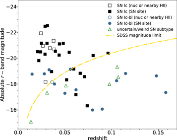
Figure 3. Absolute r-band magnitudes as a function of redshift for the host galaxies of PTF SNe Ic (black squares), SNe Ic-bl (blue circles), and weird/uncertain SN subtype transients (green triangles). For the PTF SN Ic and SN Ic-bl hosts, if the SN site is within the aperture, then closed symbols are used; otherwise, open symbols are used (for both subsets). The r-band magnitudes are global values derived from Pan-STARRS and SDSS photometry and are corrected for shredding if applicable (see text for details). Redshifts are remeasured from the spectra in this work. The SDSS legacy galaxy redshift sample has an apparent r-band magnitude limit of 17.77 mag, which is denoted by the yellow dashed–dotted curve. Sitting below the dashed curve, 2/3 of the SN Ic-bl hosts are too faint to be covered by the SDSS legacy galaxy redshift survey.
Download figure:
Standard image High-resolution imageSelected to be roughly twice the seeing disk, the aperture size used for spectrum extraction usually stays constant in angular size for all data from a given night. Since the sample of host galaxies spans a large range in luminosity and distances, this angular size corresponds to various physical scales. We check here whether this will have a significant impact on the physical sizes that we are actually probing for the SN Ic hosts as a population in comparison with the SN Ic-bl hosts, considering the fact that the hosts of SNe Ic-bl overall lie farther away (see Figure 3). The aperture size varies from 1.2 to 5.9 kpc for the SN Ic hosts with a median of 2.1 kpc and from 0.7 to 7.1 kpc for the SN Ic-bl hosts with a median of 3.0 kpc. The physical scales of the environments that we probe are on average more extended for the hosts of SNe Ic-bl than those for SNe Ic. However, both the Kolmogorov–Smirnov (K-S) test and the Anderson–Darling (A–D) test show that this difference is not statistically significant, assuming a significance level α = 0.05 (see Section 6.1). Because the hosts of SNe Ic-bl are less luminous intrinsically and are at higher redshifts, they are fainter, and thus they were all observed with Keck. The Keck runs have on average better seeing than the P200 ones, giving rise to aperture sizes in physical scales for the SN Ic-bl hosts similar to those for the nearby, more luminous SN Ic hosts observed predominantly with P200.
The SDSS main spectroscopic galaxy sample has an apparent r-band magnitude limit of 17.77 mag (Strauss et al. 2002), which is denoted by the dashed curve for different redshifts in Figure 3. Sitting below the dashed curve, ∼2/3 of the SN Ic-bl hosts are too faint to be covered by the SDSS legacy galaxy redshift survey. For the rest of our sample, presumably the hosts are bright enough so that SDSS spectra exist. However, especially the SN Ic hosts occupying the upper left part of this diagram are bright, are nearby, and thus appear large on the sky. For these galaxies, the SDSS fiber, which is 3'' in diameter, is generally centered on the galaxy nucleus, thus missing the SN site. Most isolated late-type spiral galaxies display strong metallicity gradients, being more metal-rich at the center. The spectra we present here cover the SN sites and hence are crucial for probing the immediate environments of SN explosions.
4. Comparison Samples
In this section, we define three control samples: (1) SN–GRB hosts, (2) local galaxies from the SDSS, and (3) the Local Volume Legacy Survey (LVL). We also describe how we compiled relevant observables and derived galaxy properties from the literature, which include the emission-line fluxes for the SN–GRB hosts and the SDSS galaxies, metallicities for the LVL galaxies, and global M* values and SFRs for all the samples. At the end of this section, we summarize the redshift distributions of the control samples, relative to those of the PTF SN hosts. We show that their very different redshift ranges have little impact on the intercomparison between the samples, specifically for their star formation and metallicity properties.
4.1. Hosts of SN–GRBs
Here we construct a sample of host galaxies of SN–GRBs (SN Ic-bl with an associated GRB) in order to uncover any differences in the host galaxies and environments of SNe Ic-bl with and without observed GRBs, and thus to pinpoint the physical process that gives rise to observed jets during the explosions of some massive stripped stars. If our PTF SNe Ic-bl are associated with off-axis GRBs, we expect to see no significant difference of host environments between the PTF SNe Ic-bl and SN–GRBs, since viewing-angle effects are a random process. If the PTF SNe Ic-bl in our sample have intrinsically no GRB associated with them, then there needs to be some unique property that forces GRBs to occur in some massive stripped stars in contrast to the usual SN Ic-bl without a GRB—and our environmental study could reveal what that unique property is. To distinguish between these two scenarios, we compare the host galaxies of SN–GRBs with the PTF SNe Ic-bl not having GRBs. In Section 7 we discuss whether the PTF SNe Ic-bl harbored off-axis GRBs.
For our comparison sample of SN–GRBs, we are including spectroscopically classified SN–GRBs at z < 0.3 (in order to mitigate any significant cosmic evolution for a fair comparison with the PTF SN sample) with published host galaxy data before 2018 August. There are 10 such SN–GRB hosts in the literature, which we list in Appendix B, along with their nebular emission-line fluxes that we adopt in order to compute their line ratios and metallicities with the same calibrations as we use for the PTF SN hosts (see Section 5.1). If multiple sets of flux measurements exist in the literature, we adopt the ones providing flux uncertainties, since the code we are using requires flux uncertainties for computing metallicity uncertainties (see Section 5.1). If multiple spectra are extracted from the same host at different sites, we include only the one from the SN site. We list notes for individual objects in Appendix B, and we compare the metallicities that we compute to those reported in the literature (based on the same data) in Appendix D. In Section 8, we discuss the caveats that arise from our criteria and future work that can address them. While there are GRBs within this redshift volume with no observed SNe (e.g., Dado & Dar 2018), with the most famous being GRB 060614 with very deep SN limits (e.g., Gal-Yam et al. 2006b), their classification as bona fide LGRBs is debated, as they may be short-duration GRBs in an extended tail (Ofek et al. 2007; Caito et al. 2009; Perley et al. 2009) or another type of GRB altogether (Gehrels et al. 2006; Lu et al. 2008). Indeed, their host properties are very different from those of confirmed GRB-SNe and closer to those of short GRBs (Levesque & Kewley 2007; Stanway et al. 2015).
We further compiled the M* and SFR values for these SN–GRBs from the database of GRB Host Studies (GHostS25 ) and then converted them to be consistent with the stellar IMF that we adopt for the PTF SN host sample (by adding 0.11 dex to log M* and by multiplying the SFR by a factor of 1.3; see Section 5.2), and we list them in Table 2.
The M* values were derived from SED fitting to the "pseudophotometry," that is, homogeneous photometry reconstructed by sampling the observed SEDs from the literature in a reduced set of filters (Savaglio et al. 2009). In particular, the SED is modeled as a young burst component superimposed on a population of older stars, which is more general than assuming a single simple star formation history (SFH). It yields more realistic M* estimates for the low-mass galaxies with bursty star formation behavior (Huang et al. 2012a). We applied a similar approach to obtain M* estimates for the host galaxies of PTF SNe (see Section 5.2), but we used different stellar population synthesis codes and different grids of dust extinction, stellar metallicity, etc., to generate the SED models. One of the SN–GRB hosts, GRB/XRF 060218/SN 2006aj, is detected in SDSS. We confirmed that our SED fitting process making use of the SDSS photometry yields an M* estimate consistent within 2σ with the GHostS value for this source, though our value is slightly lower. Thus, we expect no significant systematic differences in the M* estimates between our PTF SN hosts and the GRB-SN hosts.
In order to estimate the SFRs, the GHostS prefers the Hα luminosity over UV luminosity or over the luminosity of other emission lines (e.g., Hβ or [O ii]). All of the SN–GRB hosts have Hα detected, and thus their SFRs from the GHostS are based on Hα luminosity, corrected for aperture-slit loss and dust extinction. While the computed metallicities for both SN–GRBs and our PTF SN host sample reflect local values in cases where the SN site is distinct from the galaxy nucleus, the M* values and SFRs reflect global values for both the GHostS and our sample (see Section 5.2).
4.2. Galaxy Comparison Samples
In order to understand whether the SNe Ic/Ic-bl or SN–GRBs preferentially occur in certain types of galaxies over others, we select two control samples of low-redshift galaxies to set the baseline of comparison. The first sample is selected from the SDSS, which is frequently invoked in previous works of SN Ic-bl and GRB hosts to represent the overall population of star-forming galaxies (e.g., Modjaz et al. 2008a; Levesque et al. 2010b). However, the SDSS legacy galaxy redshift survey is highly incomplete below M* ≈ 108.5 M⊙ and has a fiber bias. Following Perley et al. (2016b), the second sample is selected from the LVL survey, which provides a volume-complete sample within 11 Mpc. However, limited to such a small volume, the LVL survey suffers from cosmic variance and is biased against the most massive galaxies that are rare in the local universe. Most importantly, there are no homogeneous metallicity measurements for the LVL galaxies.
An ideal control sample should have representative distributions in all physical parameters of interest to us, such as metallicity, M*, and SFR. In particular, Figure 3 shows that the hosts of SNe Ic-bl are generally of low luminosity. Inspection of their SDSS images demonstrates that many of them are dwarf irregulars barely resolved by the survey. It is therefore important to employ a control sample that is inclusive of low-mass galaxies and has star formation behavior typical of that in the local universe. Thus, the two samples that we define here are not ideal, but they are complementary for our purpose of comparison.
4.2.1. SDSS Galaxies
We select the SDSS galaxies from DR8, which is provided by the MPA-JHU catalog of galaxies, including all the main physical parameters of interest to us: M* values, SFRs, and emission-line fluxes for the metallicity calculation.
In order to self-consistently compare with our PTF SN Ic/Ic-bl hosts, we retrieve redshifts from the "galSpecInfo" table and line fluxes from the "galSpecLine" table; from the "galSpecExtra" table we get M* values, SFRs, and metallicities (calculated by Tremonti et al. 2004). The three tables contain the MPA-JHU reanalysis of all the SDSS spectra that are classified as galaxies. Note that for the PTF SN Ic/Ic-bl host galaxies we follow the approach adopted by the MPA-JHU group to obtain line flux measurements (Section 3.1.3) and M* estimates (Section 5.2). Most importantly, we derive metallicities in four calibrations from the line fluxes for the SDSS galaxies, following what we do for the PTF SN Ic/Ic-bl host galaxies (Section 5.1). Some of the calibrations are very recent and thus are not considered by the previous works that compare the SN Ic-bl and GRB hosts with the SDSS galaxies. For the SFR estimates, the MPA-JHU values that we adopt have been improved from their original values as presented by Brinchmann et al. (2004), so that the out-of-fiber SFRs are derived from SED fitting to u, g, r, i, z photometry. For the population of star-forming galaxies in particular, these MPA-JHU SFRs are consistent with the SFRs that are derived from the SED fitting involving the UV bands (Salim et al. 2016), similar to what we do for the PTF SN Ic/Ic-bl hosts (Section 5.2). Therefore, these M* values, metallicities, and SFRs for the SDSS galaxies are consistent with those for the PTF SN hosts.
In particular, the SDSS sample serves the purpose of assessing whether the PTF SN Ic/Ic-bl and SN–GRB hosts follow the same mass–metallicity (M–Z) relation as defined by the local galaxies (Section 6.3). Therefore, to select a parent sample of the SDSS galaxies, we adopt the following criteria, which are similar to those of Kewley & Ellison (2008), who derived the M–Z relation for the overall SDSS galaxies.
- 1.For reliable metallicity estimates, S/N > 8 in the strong emission lines ([O ii] λλ3726, 3729, Hβ, [O iii] λ5007, Hα, [N ii] λ6584, [S ii] λ6717, and [S ii] λ6731), following Kewley & Ellison (2008), and S/N > 3 in [O iii] λ4959.
- 2.A lower redshift limit z > 0.04, which corresponds to a flux covering fractions of >20% on average for normal star-forming galaxies observed through the 3'' SDSS fibers (Kewley & Ellison 2008). Such a covering fraction is required for metallicities to begin to approximate global values (Kewley et al. 2005). Plus, the [O ii] λλ3726, 3729 lines are not measured at z < 0.03.
- 3.The M* value derived from inside the fiber being >20% of that derived from the global photometry, to eliminate the large luminous galaxies that require a higher redshift to satisfy the covering fraction requirement.
- 4.An upper redshift limit z < 0.1, above which the SDSS star-forming sample becomes highly incomplete (Kewley et al. 2006).
- 5.A Baldwin, Phillips, & Terlevich (BPT; Baldwin et al. 1981) class of star-forming galaxy from the "galSpecExtra" table, so that the non-star-forming galaxies and the galaxies containing active galactic nuclei (AGNs) are removed.
- 6.The M* and metallicity estimates (calculated by Tremonti et al. 2004) are both available from the MPA-JHU catalog.
These selection criteria result in a parent sample of 40,879 SDSS galaxies, with a median redshift z ≈ 0.067. To select a subset that is reasonable for metallicity calculation by our code, pyMCZ (Section 5.1), we randomly sample 500 galaxies from the parent sample. We ensure that the differences are not statistically significant between the distributions of metallicities (calculated by Tremonti et al. 2004), M* values, and SFRs for this subset of 500 galaxies and those for the parent sample—that is, the subset is representative of the general SDSS population. In support of this, we can reproduce the Kewley & Ellison (2008) M–Z relation with this subset, based on the Tremonti et al. (2004) metallicities. For a comparison to galaxies hosting SNe, however, one can argue that the SDSS galaxies should not be randomly drawn, but be weighted by their SFR (Graham & Fruchter 2013), or by their sSFR. The fact that we do not do this here may explain the small offset between the SN Ic hosts and that of the unweighted SDSS galaxies to an undetermined degree. The goal here is to try to repeat what other works have done regarding the M–Z question; the community is not yet in a position to try to test fundamentally how GRBs select galaxies out of the M–Z–sSFR phase diagram. A comparison sample of SN II hosts from an untargeted transient survey is needed, since those would be tracers of hosts of massive-star explosions (e.g., K. Taggart et al. 2019, in preparation).
The SDSS legacy galaxy redshift survey is highly incomplete below M* ≈ 108.5 M⊙. While one could correct for incompleteness by applying a volume weight (e.g., Huang et al. 2012b), it is not sufficient for our purpose here because we have applied further selection criteria on emission-line fluxes, etc. The volume weight only corrects for the fact that the faint galaxies below the flux limit are missed, not for the fact that the additional galaxies are missed owing to further selection criteria.
We also note that more recent integral field unit (IFU) based M–Z calibrations have been published, including those based on the CALIFA survey (Sánchez et al. 2017) that mitigate the fiber bias of SDSS. However, since they do not extend to the low galaxy masses in which our PTF SNe Ic-bl and the SN–GRBs are found and are not calculated in the majority of the metallicity scales used in our work, we do not include them here but mention them for completeness.
4.2.2. LVL Galaxies
In contrast to the SDSS, the LVL survey provides a sample of galaxies that is complete in volume within 11 Mpc (Dale et al. 2009), dominated by dwarfs. Thus, the LVL galaxies form a better control sample than the SDSS galaxies (Perley et al. 2016b), for the comparison with the PTF SN host galaxies, especially with the hosts of SNe Ic-bl that have overall low M* values. Furthermore, the LVL catalog includes photometry from the UV to the near-infrared, yielding M* estimates from SED fitting. We adopt UV-based SFRs for the LVL sample because they are known to be more reliable than the Hα-based ones owing to stochastic star formation in the regime of low-mass galaxies (Lee et al. 2009).
However, the LVL survey is limited to only the local volume and thus suffers from cosmic variance. Moreover, the most massive galaxies that are rare in the universe are underrepresented in the local volume. Most importantly, the LVL is a photometric survey without spectroscopy; thus, there are no metallicity measurements as part of the initial survey. Metallicity measurements exist in the literature for about 2/3 of the galaxies in that sample, and we use the compilation of Perley et al. (2016b) (see also other references therein). We caution that these metallicities for the LVL galaxies are literature values in a variety of calibrations (typically electron temperature Te based at low metallicities and various strong-line diagnostics at higher metallicities), whereas for the hosts of PTF SNe and SN–GRBs, we recalculated the metallicities in various calibrations (see Section 5.1). The line fluxes for the LVL galaxies were not published, and thus we cannot run them through pyMCZ, as we do for the SN–GRB hosts. Also, these literature values were derived from spectroscopic observations that covered various fractions of the entire galaxies. Consequently, the average trends as defined by the LVL sample involving metallicities serve the purpose of only a qualitative comparison.
4.3. Redshift Distributions of the Comparison Samples
For the 10 SN–GRB hosts, the redshift distribution has zmedian = 0.146 and zaverage = 0.154, with a standard deviation of 0.104. Among them, GRB 130427A/SN 2013cq has the highest redshift (z = 0.3399). In contrast, all of the hosts of PTF SNe Ic/Ic-bl are at z < 0.158, with zmedian = 0.059 and zaverage = 0.072, with a standard deviation of 0.044. For the 500 SDSS galaxies, zmedian = 0.066 and zaverage = 0.067. Furthermore, all of the LVL galaxies lie within 11 Mpc and thus have much lower redshifts than the PTF SN or SN–GRB hosts do. We fully acknowledge that the redshift distributions of the four samples are vastly different.
However, to be able to compare these samples self-consistently, we still expect the evolutionary effect in metallicity or star formation properties to be negligible. For example, Whitaker et al. (2012) studied the redshift evolution of the SFR–mass sequence of star-forming galaxies, and the lowest redshift bin is defined to be 0.0 < z < 0.5 in that work—a redshift range that encompasses those of all of our samples. Lamareille et al. (2009) defined the same lowest-redshift bin in their study of the evolution of the M–Z relation. The evolution in the metallicity of star-forming galaxies between z ≈ 0.08 and 0.29 is less than 0.1 dex at M* ≈ 109 M⊙ (Zahid et al. 2014). In conclusion, the evolution of the average trends in the SFR–mass sequence or M–Z relation within z ≲ 0.3 is negligible relative to the observed scatter in these correlations. Although the SN–GRB hosts have overall higher redshifts than the PTF SN Ic/Ic-bl hosts and LVL members, all of these galaxies are usually considered to be local in observational studies of redshift evolution of galaxy properties.
5. Derived Host Galaxy Properties
In this section, we explain how we derive galaxy properties from observables, including the metallicities from emission-line fluxes for the SN–GRB and PTF SN Ic/Ic-bl hosts and the SDSS galaxies, as well as the M* values and SFRs from broadband photometry for the hosts of PTF SNe Ic/Ic-bl only.
5.1. Metallicity
Theoretically, metallicity is expected to influence the outcome of the deaths of massive stars as SNe or as GRBs (Heger et al. 2003). Many GRB models favor rapidly rotating massive stars at low metallicities as likely progenitors. Massive stars at low metallicities are likely to avoid losing angular momentum from mass loss, if the mass-loss rate is set by line-driven (and thus metallicity-driven) winds. However, the question will still remain how the outer stellar layers were removed at low metallicity if not by mass loss, since SNe Ic-bl (including those connected with GRBs) do not show lines of H or He.
Observationally, the metallicities of SN Ic/Ic-bl or SN–GRB progenitors can be traced by the oxygen abundance of the H ii regions at the SN sites, given that the massive progenitors have short lifetimes and thus should not move far from their birth H ii regions (see the review by Modjaz 2011, for detailed discussion and caveats). Our observations of the metallicities of SN host galaxies, measured in many cases at the SN sites, will therefore help to test such SN and GRB progenitor models.
5.1.1. Metallicity Estimation
One of the main purposes of this work is to understand the metallicity dependence in the production of different subtypes of the large family of SNe Ic: SNe Ic, SNe Ic-bl, and SN–GRBs. The nebular oxygen abundance is the canonical choice of metallicity indicator for the studies of interstellar medium (ISM), and we use these two terms (metallicity and oxygen abundance) interchangeably in this work. We recalculate the metallicities of the SN–GRB host galaxies and the subset of 500 SDSS galaxies from literature emission-line fluxes by following the same approach we applied to the PTF SN hosts in order to make a self-consistent comparison.
Two main methods of metallicity estimates can be applied to extragalactic studies: the Te-based method and the strong-line method (see a summary in Bianco et al. 2016, and the references therein). The Te-based method requires auroral lines such as [O iii] λ4363. However, the auroral lines are generally very weak, and they saturate above solar metallicity (Stasińska 2002). The strong-line methods estimate metallicities from ratios of strong nebular emission lines emitted from H ii regions.
Commonly used line ratios include the following:
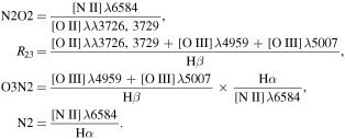
Depending on the calibration of the observed emission-line ratios, the strong-line methods can be further categorized into three types: empirical methods that are calibrated on observed Te-based metallicities, theoretical methods that are calibrated on theoretically simulated line ratios using stellar population and photoionization models, and hybrid methods that are calibrated on a mixture of the above two.
The auroral line that is needed in the Te-based method is too weak to be detected in the host galaxies of PTF SNe. Thus, we derive the metallicities from strong emission lines using an open-source Python package developed by our group, pyMCZ (Bianco et al. 2016). It is based on the original IDL code of Kewley & Dopita (2002), with updates from Kewley & Ellison (2008), and expanded to include more recent calibrations. Specifically, pyMCZ requires the emission-line fluxes and their uncertainties as inputs for Monte Carlo sampling and calculates the probability distributions (and their median and confidence intervals) of the metallicity in various calibrations. The code also calculates from the Balmer decrement the probability distribution of host galaxy extinction values, E(B − V)host, and applies internal extinction correction to the emission-line fluxes in the calculation of metallicities. In order to derive the Balmer decrement, Hα and Hβ fluxes are available for all of the host galaxies of PTF SNe and SN–GRBs.
The pyMCZ code samples the synthetic line flux measurements from a Gaussian distribution with standard deviation equal to the measurement uncertainty and centered on the measured flux value. Therefore, Bianco et al. (2016) suggest that the input lines should have an S/N of at least 3, assuring that fewer than ∼1% of the sampled fluxes fall below zero (and are thus invalid). The lines with S/N < 3 may be eliminated by setting their values to NaN in the input files to pyMCZ. The metallicity will be calculated only for the calibrations that use valid, non-NaN line fluxes. By observational design, all of our spectra have S/N > 15 in Hα and S/N > 3 in Hβ, with the only exception being PTF10aavz, which has S/N = 13.5 in Hα at the SN site. However, this does not ensure that the S/N is above 3 for all the other strong lines that we need; the N2 or R23 ratios are exceptionally low in some host spectra.
We may choose not to input the line fluxes with S/N < 3, following the suggestion of Bianco et al. (2016). However, only in a few cases is the low S/N due to noise in the spectra (e.g., the [O iii] λ5007 line of PTF10ciw falls on a night-sky line). For the rest, the low S/N is caused by that line being particularly weak relative to the Balmer lines. For example, the N2 ratio is sensitive to ionization parameter, but to first order, a low N2 ratio indicates a low metallicity. As a result, eliminating the [N ii] line with S/N < 3 generally causes a bias against the most metal-poor systems in the calibrations that require [N ii] flux for calculation. Four of the PTF SN hosts have S/N < 3 in [N ii] λ6584—two of SNe Ic-bl (PTF10qts, PTF10tqv) and the other two of SNe Ic (PTF10hie, PTF11rka)—and all are computed to be metal-poor. Similarly, in the metal-rich regime of log (O/H) + 12 ≳ 8.7, the lower the R23 ratio, the higher the metallicity (e.g., Kewley et al. 2004). Eliminating the [O ii] or [O iii] lines with S/N < 3 generally causes a bias against the most metal-rich systems.
Therefore, we choose to input NaN to pyMCZ only if the lines are outside of the wavelength coverage (including the [O ii] lines for PTF10bip, PTF12gzk, and PTF12hni) or are not detected at all (including both [O iii] lines for PTF10qqd and PTF10yow). They appear as missing values in Appendix A. For the lines detected with S/N < 3, we keep their flux measurements as derived by platefit in the input files to pyMCZ. The pyMCZ code has been modified to properly deal with input lines that have S/N < 3 since it sets invalid negative synthetic line fluxes to zero during sampling, and we check whether a sufficient sample size is retained from 2000 Monte Carlo trials to build the final distribution of the metallicity.
5.1.2. Metallicity Calibrations
Different metallicity calibrations give systematically different metallicity values, even based on the same line fluxes (e.g., Kewley & Ellison 2008), and there is no consensus on which calibration to use. In order to make sure our results are independent of the chosen metallicity calibration, we present our analysis with four different calibrations that are relatively independent. To decide which calibrations we should present, we examine the intercomparisons between the metallicity values based on our data for all the calibrations implemented by pyMCZ (over 23 of them; for a full definition of the calibrations see Bianco et al. 2016, and references therein).
Although available through pyMCZ, some older calibrations, such as M91 (McGaugh 1991) and Z94 (Zaritsky et al. 1994), are obsolete. We evaluate the performance of the remaining metallicity calibrations in a data-driven fashion, and we do not report metallicities for the calibrations that generally produce measurements with large scatter compared to the results in most of the other calibrations for our 48 PTF SN hosts: that includes M08_O3O2 (Maiolino et al. 2008) and P10_ON and P10_ONS (Pilyugin et al. 2010). In addition, we chose a single calibration for each metallicity diagnostic (set of line ratios). For example, several calibrations are based on N2: D02 (Denicoló et al. 2002), PP04_N2Hα (Pettini & Pagel 2004), KK04_N2Hα (Kobulnicky & Kewley 2004), and M08_N2Hα (Maiolino et al. 2008). We only present the result for one of them, M08_N2Hα. Similarly, where there is more than one calibration based on the same theoretical model, which thus should deliver self-consistent metallicities, we present only one. For example, eight calibrations from Dopita et al. (2013) can be calculated with pyMCZ and our line inputs, but we only present the result for one of them, D13_N2S2_O3S2.
In summary, we choose to present the median values, 16th percentiles, and 84th percentiles of our metallicities, together with E(B − V)host estimates, in the four calibrations KD02comb, D13_N2S2_O3S2, PP04_O3N2, and M08_N2Hα. Table 3 contains these values for the hosts of PTF SNe Ic/Ic-bl (including the six weird/uncertain SN subtype transients). Table 2 contains the same values for the hosts of SN–GRBs. We calculate them using pyMCZ in the same manner for both data sets to make a fair comparison. Among these four calibrations, KD02comb and D13_N2S2_O3S2 are theoretical, while PP04_O3N2 and M08_N2Hα are hybrid. We note that none of them are empirical, calibrated purely on the Te-based metallicities. Historically, there have been large systematic offsets between the Te-based and theoretical calibrations.
Table 2. SN–GRB Hosts: M* and SFR from Literature and Our PYMCZ Computations for Reddening and Metallicities
| SN–GRB Name | log M*a | SFRa | E(B − V)host | log (O/H) + 12 | log (O/H) + 12 | log (O/H) + 12 | log (O/H) + 12 |
|---|---|---|---|---|---|---|---|
| (M⊙) | (M⊙ yr−1) | (mag) | D13_N2S2_O3S2 | KD02_COMB | PP04_O3N2 | M08_N2Hα | |
| GRB 980425/SN 1998bw | 8.79 ± 0.30 | 0.338 ± 0.08 |

|

|

|

|

|
| XRF 020903 | 8.98 ± 0.07 | 3.445 |

|

|

|

|

|
| GRB 030329/SN 2003dh | 7.85 ± 0.06 | 0.143 |

|

|

|

|

|
| GRB 031203/SN 2003lw | 8.93 ± 0.43 | 16.484 |

|
⋯ |

|

|

|
| GRB/XRF 060218/SN 2006aj | 7.89 ± 0.08 | 0.065 |

|

|

|

|

|
| GRB 100316D/SN 2010bh | 9.04 | 0.182 |

|

|

|

|

|
| GRB120422A/SN 2012bz | 9.06 ± 0.04 | 0.52 ± 0.10 |

|

|

|

|

|
| GRB 130427A/SN 2013cq | 9.43 ± 0.15 | 1.17 ± 0.10 |

|

|

|

|

|
| GRB 130702A/SN 2013dx | 8.01 ± 0.70 | 0.065 |

|
⋯ | <8.20 | ⋯ | <8.37 |
| GRB 161219B/SN 2016jcab | 8.88 ± 1.03 | 0.25 ± 0.30 |

|
⋯ |

|

|

|
Notes.
aTaken from the GHosts database (consult it for original data references), unless otherwise indicated for GRB 161219B/SN 2016jca, and converted to be consistent with our adopted Chabrier IMF (by adding 0.11 dex to log M* and by multiplying the SFR by a factor of 1.3; see Section 5.2). bFor GRB 161219B/SN 2016jca, the M* and SFR were taken from Cano et al. (2017a).Download table as: ASCIITypeset image
Table 3. pyMCZ Measurements
| PTF Name | SN Type | E(B − V)host | log (O/H) + 12 | log (O/H) + 12 | log (O/H) + 12 | log (O/H) + 12 |
|---|---|---|---|---|---|---|
| (mag) | D13_N2S2_O3S2 | KD02_COMB | PP04_O3N2 | M08_N2Hα | ||
| SN Ic-bl | ||||||
| 09sk | Ic-bl |

|

|

|

|

|
| 10aavz | Ic-bl |

|

|

|

|

|
| 10bzf/SN10ah | Ic-bl |

|

|

|

|

|
| 10ciw | Ic-bl |

|

|

|

|

|
| 10qts | Ic-bl |

|

|

|

|

|
| 10tqv | Ic-bl |

|

|

|

|

|
| 10vgv | Ic-bl |

|

|

|

|

|
| 10xem | Ic-bl |

|
⋯ |

|

|

|
| 11cmh | Ic-bl |

|

|

|

|

|
| 11gcj | Ic-bl |

|

|

|

|

|
| 11img | Ic-bl |

|

|

|

|

|
| 11lbm | Ic-bl |

|

|

|

|

|
| 11qcj | Ic-bl |

|

|

|

|

|
| 12as | Ic-bl |

|

|

|

|

|
| SN Ic | ||||||
| 09iqd | Ic |

|

|

|

|

|
| 10bhu | Ic |

|

|

|

|

|
| 10fmx | Ic |

|

|

|

|

|
| 10hfe | Ic |

|

|

|

|

|
| 10hie | Ic |

|

|

|

|

|
| 10lbo | Ic |

|

|

|

|

|
| 10ood | Ic |

|

|

|

|

|
| 10osn | Ic |

|

|

|

|

|
| 10qqd | Ic |

|
⋯ |

|
⋯ |

|
| 10tqi | Ic |

|

|

|

|

|
| 10wal | Ic |

|

|

|

|

|
| 10xik | Ic |

|

|

|

|

|
| 10yow | Ic |

|
⋯ |

|
⋯ |

|
| 10ysd | Ic |

|

|

|

|

|
| 10zcn | Ic |

|

|

|

|

|
| 11bov/SN11bm | Ic |

|

|

|

|

|
| 11hyg/SN11ee | Ic |

|

|

|

|

|
| 11ixk | Ic |

|

|

|

|

|
| 11jgj | Ic |

|

|

|

|

|
| 11klg | Ic |

|

|

|

|

|
| 11rka | Ic |

|

|

|

|

|
| 12cjy | Ic |

|

|

|

|

|
| 12dcp | Ic |

|

|

|

|

|
| 12dtf | Ic |

|

|

|

|

|
| 12fgw | Ic |

|

|

|

|

|
| 12hvv | Ic |

|

|

|

|

|
| 12jxd | Ic |

|

|

|

|

|
| 12ktu | Ic |

|

|

|

|

|
| Weird/Uncertain SN Subtype | ||||||
| 09ps | Ic/Ic-bl |

|

|

|

|

|
| 10bip | Ic/Ic-bl |

|

|
⋯ |

|

|
| 10gvb | SLSN/Ic-bl |

|

|

|

|

|
| 10svt | Ib/c |

|

|

|

|

|
| 12gzk | Ic-peculiar |

|

|

|

|

|
| 12hni | SLSN/Ic-bl |

|

|

|

|

|
Download table as: ASCIITypeset image
In Appendix C, we briefly describe pertinent details of each of the four calibrations we adopt.
There is a long-standing debate about which metallicity calibration should be used, and there are known systematic offsets between the various calibrations (see Kewley & Ellison 2008). Having chosen four calibrations that best fit our needs, we are not generally advocating for the use of these over others. Moreover, it should be noted that the pyMCZ code does not include systematic errors between the calibrations, so the reader should refrain from absolute comparisons of calibrations and especially from comparing galaxies across different calibrations. The metallicity uncertainties presented here are statistical ones and account for the flux uncertainties and calibration uncertainties if provided. The four calibrations are chosen to represent a variety, so as to test whether any trends that we see are calibration dependent. Although the absolute metallicity values vary depending on the calibration used, the relative metallicity trends can be robust and thus should be seen across different calibrations if the analysis is performed self-consistently for the same calibration (Kewley & Ellison 2008).
5.2. Stellar Masses and SFRs
As described in Section 3.2, we compile broadband UV to optical photometry with good quality for all 48 PTF SN host galaxies (SDSS u, g, r, i, z for 44 hosts, Pan-STARRS g, r, i, z for 4 hosts, and GALEX FUV and NUV bands for 36 hosts). We present these magnitudes with uncertainties in Table F.1 (including the six weird/uncertain SN subtype transients), corrected for Galactic extinction. In this section, we derive the global M* values and SFRs of these host galaxies via SED fitting and list them in Table F.1. More details of the SED fitting process, which follows the method of Salim et al. (2007), are provided by Huang et al. (2012a) and Huang et al. (2012b). We adopt the same SED models as the ones used by the MPA-JHU group, so that the M* values of the PTF SN Ic/Ic-bl hosts are fully consistent with those that we retrieve from the MPA-JHU catalog for the SDSS galaxies (see Section 4.2.1). We also expect no significant systematic offsets of the M* and SFR values between those derived in this work for the PTF SN Ic/Ic-bl hosts and those compiled from the literature for SN–GRB hosts (see below).
We use a library of 100,000 SED models generated with the Bruzual & Charlot (2003) stellar population synthesis code (Gallazzi et al. 2005), assuming a Chabrier (2003) IMF. Dust is accounted for with the Charlot & Fall (2000) two-component model to include attenuation from both the diffuse ISM and short-lived (10 Myr) giant molecular clouds. A grid of models with an extensive range of stellar metallicity (correlated but different from the gas-phase metallicity as derived in Section 5.1), internal extinction, and SFHs are considered. The stellar metallicity range is 0.1–2.0 solar, and the effective optical depth in the V band, τV, is 0–6. The prior on the distribution of the stellar metallicity is uniform, and that of τV is Gaussian with a standard deviation of 0.55 dex and a mean predicted by Giovanelli et al. (1995), being higher in more massive galaxies and in more inclined galaxies.
A common way to model the SFH is to parameterize it as a smoothly declining exponential, SFH(t; T) = e−t/T, where T is the timescale of the decay, and then calculate a grid in T. The library of SED models that we use is generated following an alternative approach that mimics stochastic processes in which the SFHs are drawn randomly according to some prior assumptions. This technique was introduced for galaxy-parameter estimation by Kauffmann et al. (2003) and is widely used by Gallazzi et al. (2005), Salim et al. (2007), the MPA-JHU group, and others to estimate M* based on the fit to the SDSS photometry. The stochastic effect in star formation may be significant in low-mass galaxies (Lee et al. 2009), and hence the stochastic model, which allows for a wide range of SFHs, is more realistic. In particular, it allows random bursts in SFH that are superimposed on a continuous component. Similarly, for the M* estimates of SN–GRB hosts, we adopt the GHostS values for which the estimation is discussed by Savaglio et al. (2009), who also model the SFH as a young burst component superimposed on a population of older stars, but we convert them such that the adopted IMF is consistent with the one we use by adding 0.11 dex to log M*. However, we note that such methods that include bursts in the SFHs generally result in systematically smaller M* estimates than if assuming a smooth exponential SFH (e.g., Bell et al. 2003). The difference increases with decreasing M* to be ∼0.4 dex on average at M* = 108 M⊙ (Wyder et al. 2007), because the difference is more significant in the galaxies with higher ratios of current to past-averaged SFRs, which many low-mass galaxies have.
Given the SED models, we follow a Bayesian approach to estimate galaxy parameters, such as M* and SFR, by deriving posterior probability density functions (PDFs) from the PDFs that are computed based on priors (the galaxy parameters are known for the models) and the likelihood functions. Assuming Gaussian errors in the flux, the likelihood of data given each model is calculated by minimizing the χ2 of the fit. By convention, all of the models are normalized to have a total of 1 M⊙ in M* formed by the present day. For each model, M* is essentially derived from a scaling factor to minimize the χ2 between the model fluxes and the observed magnitudes (see, e.g., Salim et al. 2007). Owing to the stochastic nature of the star formation behavior in our adopted models, the physical parameters associated with a single best-fit model with the maximum likelihood (the best χ2) might lead to peculiar results at times. We therefore generate a full marginalized posterior PDF for each physical parameter. For the M* and SFR estimates of all 48 PTF SN hosts, we report the median values from such distributions in Appendix F, along with the uncertainties denoting the 16th and 84th percentiles from distributions.
We now describe how we calculate SFRs for the models of galaxies, the physical meaning of this definition, as well as why the SFRs derived in this way (SED fitting) are consistent with those of comparison samples. For each model of a galaxy, the SFR is derived from averaging the SFH over the past 100 Myr. A UV-bright star has a lifetime of ∼100 Myr, and thus the UV luminosity as an SFR indicator also probes a timescale of ∼100 Myr. For 36 of the PTF SN host galaxies with GALEX magnitudes, the SED fitting is applied to UV to optical bands; therefore, their SFRs averaged over the past 100 Myr are based on UV luminosity to first order. Similarly, the SFRs of LVL galaxies that we adopted are also based on UV luminosity. We note, however, that the SFRs of SN–GRB hosts are based on Hα, which traces a more instantaneous timescale (∼10 Myr). It was found among low-mass galaxies from the LVL survey that Hα tends to increasingly underpredict the total SFR relative to the FUV, probably owing to stochasticity in the formation of high-mass stars (Lee et al. 2009). However, this trend only becomes evident for galaxies with SFR ≲ 0.01 M⊙ yr−1, whereas all of the host galaxies we consider in this work have SFR > 0.01 M⊙ yr−1, and most of them have SFR > 0.1 M⊙ yr−1. Accordingly, we think that it is fair to compare the Hα-based SFRs of SN–GRB hosts with the FUV-based SFRs of PTF SN hosts and LVL galaxies. In addition, we conducted a comparison between Hα-based and NUV-based SFR estimates using our work, that of Savaglio et al. (2009), and that of Kelly et al. (2014) and find that in all cases (hosts of two SN–GRBs, four PTF SNe Ic-bl, and five PTF SNe Ic) the values are consistent with each other within 1σ.
For the PTF SN hosts without GALEX magnitudes, our SED fitting process is applied to optical-only bands. Their SFRs are poorly constrained, especially for the two hosts outside of both SDSS and GALEX (PTF09iqd and PTF10svt, with neither u nor FUV/NUV magnitudes). This effect is reflected in the broader posterior PDFs for their SFR estimates and thus gives rise to higher SFR uncertainties. In the following figures that involve SFRs, we plot the PTF SN Ic/Ic-bl hosts without GALEX magnitudes by open symbols, indicating that their SFRs are less reliable. In contrast, the M* derived from a scaling factor is well constrained by SED fitting to optical-only bands and is insensitive to the extra UV data.
6. Results
In this section, we compare the distributions of various physical parameters derived in the previous section for the PTF SN Ic/Ic-bl hosts with those for the SN–GRB hosts and LVL galaxies, in order to address the question whether the SNe Ic-bl or SN–GRBs preferentially occur in certain types of galaxies over others from comparison samples and what these preferences are (if any). Such constraints from the environment will help to test the formation models of SNe Ic-bl and SN–GRBs, which we undertake in Section 7.
6.1. BPT Diagram
We explore the distributions of host galaxies across a BPT diagram, in order to (i) identify the ones having an AGN contribution, so that the quantities derived from emission lines should be taken as approximate; (ii) compare the line-ratio distributions between the hosts of different SN populations; and (iii) study the implications for metallicity, ionization, and age conditions, which together predict a certain location in the diagram (e.g., Dopita et al. 2000), given the different parameter spaces occupied by samples.
6.1.1. Identifying AGNs
The BPT diagram was first proposed by Baldwin et al. (1981) to separate the main excitation mechanism of emission-line objects via the line ratios of [O iii] λ5007/Hβ versus [N ii] λ6584/Hα. The bottomleft panel in Figure 4 shows a BPT diagram for the hosts of PTF SNe Ic/Ic-bl and SN–GRBs. The lower solid line in the BPT diagram is an empirical division derived from SDSS galaxies in Kauffmann et al. (2003), and the upper dashed line is a theoretical upper limit for pure starburst models from Kewley et al. (2001). They are usually invoked to distinguish between classical star-forming objects (below the solid line), AGN-powered sources (above the dashed line), and composite objects (in between the two lines).
Figure 4. BPT diagram for the hosts of PTF SNe Ic (black squares), PTF SNe Ic-bl (blue circles), SN–GRBs (red diamonds), and weird/uncertain SN subtype transients (green triangles), as well as for a representative sample of SDSS galaxies (yellow crossed circles). The top and right panels show cumulative distributions of the two line ratios (respectively) for the hosts of PTF SNe Ic (black dotted line), PTF SNe Ic-bl (blue dashed line), SN–GRBs (red solid line), and the SDSS galaxies (yellow solid line). The flux uncertainties are denoted by error bars in the diagram and by colored bands in the side and top panels. The gray curves in the BPT diagram show the separation between star-forming galaxies (below the solid curve), composite galaxies (in between the solid and dashed curves), and galaxies whose spectra have a significant AGN contribution (above the dashed curve). All of the host galaxies in our sample can be safely classified as star-forming, except for GRB 031203/SN 2003lw, which is at the intersection of the three regions (open diamond; see discussion in text).
Download figure:
Standard image High-resolution imageThe ionization source for all the host galaxies in our PTF SN and SN–GRB samples is star formation rather than AGN activity, except potentially for the host of GRB 031203/SN 2003lw. Thus, the strong-line methods that we adopt for metallicity calculations are valid for almost all of the hosts in our sample; so are the Hα-based SFRs for SN–GRB hosts in particular. However, the AGN contamination may render the metallicity and SFR measurements incorrect for the host of GRB 031203/SN 2003lw. We present our analysis results with and without this object and plot it with a different symbol, in order to assess its impact. See Appendix E for more details on the classification of all host galaxies, especially why we cannot rule out AGN contamination for the host of GRB 031203/SN 2003lw.
6.1.2. Line Flux Ratios
The analysis of line flux ratios is a model-independent diagnostic; thus, line-ratio plots are an important diagnostic tool. Before we study what the line ratios imply in terms of the metallicity, ionization, and age conditions, which are all model-dependent quantities, we can make a direct comparison of the line-ratio distribution between our samples to assess statistical differences.
In the bottom left panel of Figure 4, the hosts of PTF SNe Ic are represented by black squares, SNe Ic-bl by blue circles, and SN–GRBs by red diamonds. For the hosts of SNe Ic and SNe Ic-bl, open (not filled) symbols indicate that the SN sites are outside of the apertures for spectral extraction. Among both samples, the open symbols do not systematically deviate from the closed ones; the metallicities of the regions that are less representative of the SN local environments are not significantly different from those that are representative. The hosts of SNe Ic occupy the full range of the sequence, whereas the hosts of SNe Ic-bl and SN–GRBs belong exclusively to the upper left half of the sequence. The difference between the hosts of SNe Ic-bl and SN–GRBs is more subtle. We therefore perform a quantitative comparison between the samples by investigating the two line ratios separately.
In the top and right panels of Figure 4, we respectively compare the empirical cumulative distribution functions (CDFs) of the three samples for these two line ratios. The colored bands denote 1σ flux measurement uncertainties. For each sample, the CDF includes both open and closed symbols from the plot in the bottom left panel. Note that the two SN Ic hosts with no detections in [O iii] λ5007 show up only in the top panel for [N ii] λ6584/Hα. The host of GRB 130702A/SN 2013dx, which has no detection in [O iii] λ5007 and an upper limit in [N ii] λ6584, also shows up only in the top panel: it appears as a value associated with an arrow pointing to the left.
Considering these upper limits, we should describe the CDF of [N ii] λ6584/Hα for SN–GRBs by the Kaplan–Meier estimator, which uniformly distributes the weight of each upper limit among the detections with lower values. In the absence of censored data (lower or upper limits), the Kaplan–Meier estimator reduces to the usual CDF. We use the ASURV package for survival analysis (Lavalley et al. 1992) to calculate the Kaplan–Meier estimator. However, new methods are still needed that combine the virtues of survival analysis and measurement errors (Lavalley et al. 1992). In order to demonstrate how the differences in distributions compare with the typical measurement errors, we choose to plot the usual CDF rather than Kaplan–Meier estimator for SN–GRBs in the top panel by treating the upper limit as uncensored data but indicating it by an arrow.
In the top panel, the overall [N ii] λ6584/Hα ratios for the three samples follow the order of SN–GRB < SN Ic-bl < SN Ic, though this trend has not yet been statistically tested for actual significance. In the right panel, the overall [O iii] λ5007/Hβ ratios for the three samples follow the order of SN Ic < SN Ic-bl < SN–GRB, though the significance of this trend has also not yet been statistically tested. For both line ratios, the differences between the CDFs of SN Ic and SN Ic-bl hosts are much higher than the 1σ measurement errors (colored bands), but those between the CDFs of SN Ic-bl and SN–GRB hosts are less so. For the [N ii] λ6584/Hα ratio in particular, the CDF offset between the hosts of SNe Ic-bl and SN–GRBs can be largely explained by measurement errors.
Thus, in order to assess whether the differences in line-ratio distributions are significant, we perform statistical tests. The tests account for the fact that the CDFs are based on our data, which do not sample the full underlying populations, but the tests do not account for the measurement errors. For each pair of the samples that are adjacent in the sequence of SN Ic, SN Ic-bl, and SN–GRB, we test the null hypothesis that their line ratios are drawn from the same underlying distribution. The ASURV package applies the Logrank test and various generalized Wilcoxon tests on censored data, but the Logrank test can only be used when observations are censored. To be consistent, we report results of the Peto & Peto generalized Wilcoxon test for censored data and apply the Wilcoxon rank sum test with scipy in the absence of censored data. Our conclusion is based on computing the p-value, which is the probability of obtaining an effect at least as extreme as the one observed assuming the truth of the null hypothesis. Throughout this work, we choose a significance level α = 0.05, which indicates a 5% risk of concluding that a difference exists when there is no actual difference (i.e., Type I error). If the p-value we obtain is less than or equal to this significance level, we reject the null hypothesis—that is, we conclude that the difference is statistically significant at the 2σ level.
Between the samples of SN Ic and SN Ic-bl hosts, the p-value of the Wilcoxon rank sum test on the distributions of [N ii] λ6584/Hα ratios is very close to zero and that on the distributions of [O iii] λ5007/Hβ ratios is 0.002 (<0.05).
Now we turn to the important case of comparison between the SN Ic-bl and SN–GRB hosts. If GRB 031203/SN 2003lw with a potential AGN contribution is included in the SN–GRB sample, the p-value of the Peto & Peto generalized Wilcoxon test on the distributions of the [N ii] λ6584/Hα ratio is 0.210 (>0.05), but that of the Wilcoxon rank sum test on the distributions of the [O iii] λ5007/Hβ ratio is 0.022 (<0.05). However, if GRB 031203/SN 2003lw is excluded, the same p-values are 0.26 and 0.08 (both >0.05), respectively, for the [N ii] λ6584/Hα and [O iii] λ5007/Hβ ratios. Owing to the fact that the GRB 031203/SN 2003lw host has a high [O iii] λ5007/Hβ ratio and that the Wilcoxon rank sum test is sensitive to the difference in the tails of the distributions, the null result is reliable for the comparison between the [O iii] λ5007/Hβ ratios of the SN Ic-bl and SN–GRB hosts excluding potential AGNs.
To conclude, we infer from our data that the differences in line-ratio distributions between the populations of SN Ic and SN Ic-bl hosts are statistically significant, but not those between the SN Ic-bl and SN–GRB hosts, especially if the host that may harbor potential AGNs is excluded. We have applied several other hypothesis tests, including the Logrank test and various Generalized Wilcoxon tests on censored data, as well as the K-S test and the A–D test on uncensored data. All of them reach the same conclusion, except for the tests on the [O iii] λ5007/Hβ ratios between the SN Ic-bl and SN–GRB hosts, if potential AGNs are included. However, we note that the small sample sizes of both the SN Ic-bl and SN–GRB hosts may affect the power of these tests, leading to a higher Type II error rate in the presence of inherently different populations.
Even if additional correction for stellar absorption is applied to the SN–GRB hosts, it has little impact on the CDF of [N ii] λ6584/Hα, since the correction is low for Hα. Given a sample of 46 GRB hosts (only five of them are SN–GRB hosts), Savaglio et al. (2009) derive the mean correction for Hα to be 4%, which, if applied to all of our SN–GRB hosts, would suggest a shift in CDF for SN–GRBs by only 0.02 dex to the left in the top panel of Figure 4. However, as the overall correction for Hβ is higher, the CDF of [O iii] λ5007/Hβ for SN–GRB hosts would shift more in the right panel (downward by 0.08 dex, assuming a 20% correction for Hβ from Savaglio et al. 2009, derived from the full sample of GRB hosts), and therefore it would appear even closer to that of SN Ic-bl hosts. This consideration strengthens our result that we find no significant difference in the line-ratio distributions between SN Ic-bl and SN–GRB hosts.
6.1.3. Implications for Physical Parameters of Galaxies Hosting SNe
In order to interpret observed line ratios, various theoretical works have combined stellar population synthesis with photoionization models to predict line ratios, given variations in the metallicity, ionization parameter, electron density, and SFH (e.g., Dopita et al. 2000; Kewley et al. 2001). In particular, expected grids of constant metallicities and ionization parameters have been overlaid on a BPT diagram, with all the other parameters fixed—for example, grids calculated based on instantaneous zero-age starburst models or on continuous starburst models. In these works, a well-known degeneracy exists such that a given location in the BPT diagram can be explained by different combinations of metallicity and ionization parameters, especially for continuous starburst models (e.g., Kewley et al. 2001). Therefore, it appears that only when fixing one of the two parameters involved in the grid (metallicity or ionization parameter) is it possible to derive a trend with the other parameter across the BPT diagram.
On the other hand, observations show that the more metal-poor H ii regions are generally located in the upper left corner of the diagram and the more metal-rich ones are located toward the lower right corner (e.g., Sánchez et al. 2015), which cannot be explained purely by the theoretical grids. In fact, the metallicity is observed to anticorrelate with ionization parameter (e.g., Dopita & Evans 1986; Perez-Montero 2014, with metallicities derived from Te), so that not any arbitrary combination of the two is allowed by nature. For example, given the model grids calculated by Kewley et al. (2001) that assume continuous starbursts, the upper left corner (−1, 0.5) can be explained either by a model with a supersolar metallicity but extremely high ionization parameter or by a model with a subsolar metallicity and moderate ionization parameter. The former model is unrealistic owing to the anticorrelation between the metallicity and ionization parameter, and thus the upper left corner is generally associated with metal-poor H ii regions. In a BPT diagram, the parameter space populated by real H ii regions is therefore much more restricted than that predicted by model grids (see the narrow sequence in Figure 4, though the exact location depends on redshift; e.g., Erb et al. 2006; Shapley et al. 2015). More importantly, after the models with unrealistic combinations of the two parameters are excluded, the rest define a cleaner trend of the increasing metallicity from the upper left to the lower right corner along the sequence. Such a trend sets the foundation of some strong-line methods, which derive metallicities from the line ratios like O3N2 and N2 in certain ranges monotonically. Similarly, an overall trend of decreasing ionization parameter from the upper left to the lower right along the sequence is observed (e.g., Sánchez et al. 2015).
Based on this understanding, we can infer the average trends of gas-phase metallicities and ionization parameters for the hosts of PTF SNe Ic, PTF SNe Ic-bl, and SN–GRBs as populations by comparing their distributions on a BPT diagram in Figure 4, regardless of the apparent degeneracy in model grids. Furthermore, Sánchez et al. (2015) link a location on the BPT diagram to the average age and metallicity of the underlying stellar populations derived from the CALIFA observations. They find that [N ii] λ6584/Hα increases with increasing stellar age and stellar metallicity, whereas [O iii] λ5007/Hβ decreases with increasing stellar age and stellar metallicity. We can therefore infer the properties of underlying stellar populations of the hosts as well by comparing their distributions of line ratios.
We find that the hosts of SNe Ic occupy the full range of the sequence, whereas the hosts of SNe Ic-bl and SN–GRBs belong exclusively to the upper left half of the sequence. In our samples, there seems to be an upper limit in the metallicity of host environment for the formation of SNe Ic-bl and SN–GRBs. In the side panels, the CDFs indicate that the overall metallicities for the three samples appear to follow the order of ZGRB < ZIc-bl < ZIc and that the overall ionization parameters appear to follow the opposite order of qIc < qIc-bl < qGRB. Regarding the underlying stellar populations, the overall metallicities and ages follow the order of SN–GRB < SN Ic-bl < SN Ic. However, these trends have not yet been statistically tested for actual significance, which we perform below. We note that such qualitative trends are implied by the overall physical conditions of H ii regions observed along the sequence, even without having computed model-dependent values for the quantities of interest, such as metallicity and ionization parameter. We will present direct comparisons of the derived quantities like metallicities in the following sections, as well as test for the significance of the differences between the populations.
6.2. Metallicity Distribution
In this section, we compare the metallicity distributions in four calibrations for the samples of PTF SN Ic, PTF Ic-bl, and SN–GRB hosts, in order to uncover any differences between the samples. We also compare the metallicity distributions for the same sample across different calibrations, to uncover any biases in these calibrations and their possible impact on our conclusions.
6.2.1. Statistics of the Distributions
The statistics of the metallicity distributions are summarized in Table 4 for each sample and in the four calibrations (D13_N2S2_O3S2, KD02_COMB, PP04_O3N2, and M08_N2Hα), which were chosen for reasons given in Section 5.1. Owing to possible AGN contamination to the hosts of GRB 031203/SN 2003lw and GRB 091127/SN 2009nz, we consider both the cases with and without them in the SN–GRB sample. For the KD02comb, PP04_O3N2 (if potential AGNs are included), and M08_N2Hα calibrations, the SN–GRB sample contains one upper limit (because of GRB 130702A/SN 2013dx), so these statistics are calculated using the ASURV package Kaplan–Meier estimators.
Table 4. Metallicity Distributions in Various Calibrations for the Different Host Samples
| SN Type | N | Mean | SEM | 25th | Median | 75th |
|---|---|---|---|---|---|---|
| D13_N2S2_O3S2 | ||||||
| PTF SN Ic | 26 | 8.782 | 0.08 | 8.677 | 8.867 | 9.103 |
| PTF SN Ic-bl | 13 | 8.373 | 0.067 | 8.152 | 8.363 | 8.545 |
| SN Ic-bl+GRB (excluding potential AGN) | 7 | 8.211 | 0.137 | 8.163 | 8.343 | 8.375 |
| KD02_COMB | ||||||
| PTF SN Ic | 28 | 8.779 | 0.055 | 8.73 | 8.828 | 8.938 |
| PTF SN Ic-bl | 14 | 8.421 | 0.062 | 8.242 | 8.48 | 8.57 |
| SN Ic-bl+GRB (including potential AGN)a | 10 | 8.339 | 0.071 | 8.115 | 8.183 | 8.515 |
| SN Ic-bl+GRB (excluding potential AGN)a | 9 | 8.304 | 0.070 | 8.107 | 8.160 | 8.479 |
| PP04_O3N2 | ||||||
| PTF SN Ic | 26 | 8.594 | 0.048 | 8.515 | 8.642 | 8.774 |
| PTF SN Ic-bl | 14 | 8.318 | 0.036 | 8.266 | 8.308 | 8.400 |
| SN Ic-bl+GRB (including potential AGN) | 9 | 8.202 | 0.058 | 8.066 | 8.259 | 8.329 |
| SN Ic-bl+GRB (excluding potential AGN) | 8 | 8.219 | 0.063 | 8.098 | 8.282 | 8.344 |
| M08_N2Hα | ||||||
| PTF SN Ic | 28 | 8.810 | 0.058 | 8.781 | 8.898 | 8.972 |
| PTF SN Ic-bl | 14 | 8.480 | 0.057 | 8.353 | 8.486 | 8.669 |
| SN Ic-bl+GRB (including potential AGN)a | 10 | 8.295 | 0.110 | 8.068 | 8.282 | 8.521 |
| SN Ic-bl+GRB (excluding potential AGN)a | 9 | 8.287 | 0.124 | 7.917 | 8.298 | 8.535 |
Note.
aContaining an upper limit (GRB 130702A/SN 2013dx).Download table as: ASCIITypeset image
The sample sizes (Column (2) in Table 4) are calibration dependent. Among these four calibrations, KD02comb and M08_N2Hα are the ones computable for all of the hosts in our samples: 28 SNe Ic, 14 SNe Ic-bl, and 10 SN–GRBs (including potential AGNs). Assuming a solar metallicity of log(O/H) + 12 = 8.69 (Asplund et al. 2009), the mean metallicities for the hosts of SNe Ic, SNe Ic-bl, and SN–GRBs excluding potential AGNs are in the ranges of 0.80–1.32 Z⊙, 0.42–0.62 Z⊙, and 0.33–0.41 Z⊙, respectively, across the four scales. Alternatively, assuming a solar metallicity of log(O/H) + 12 = 8.76 ± 0.07 (Caffau et al. 2011), the same values are in the ranges of 0.68–1.12 Z⊙, 0.36–0.52 Z⊙, and 0.28–0.35 Z⊙, respectively. Both the mean and median values show that the metallicities of the three samples follow the sequence of ZGRB < ZIc-bl < ZIc, which agrees with the implication from line ratios, though these trends have not yet been statistically tested for actual significance. The mean and median metallicities for the SN Ic hosts are about solar, but those for the SN Ic-bl and SN–GRB hosts are well below solar. The average differences between the SN Ic and SN Ic-bl hosts range from 0.28 dex (PP04_O3N2) to 0.41 dex (D13_N2S2_O3S2).
The average differences between the SN Ic-bl and SN–GRB hosts (excluding potential AGNs) range from only 0.10 dex (in PP04_O3N2) to 0.19 dex (in M08_N2Hα), which are comparable to the standard errors of sample means (SEMs), as listed in Table 4. With the smallest size, the sample of SN–GRB hosts always has the highest SEM among the three (from 0.06 dex for PP04_O3N2 to 0.14 dex for D13_N2S2_O3S2). Columns (5) and (7) list the 25th and 75th percentiles, respectively, and their difference characterizes the standard deviation of the distribution. For the only calibration without upper limits (D13_N2S2_O3S2), the SN Ic sample has the highest standard deviation—that is, SNe Ic occur in galaxies with a large range of metallicities, whereas SNe Ic-bl and SN–GRBs from our samples occur exclusively in galaxies with low metallicities.
6.2.2. Statistical Tests on Distributions
In this section, we apply hypothesis tests on the metallicity distributions to determine whether the observed differences between the hosts of SNe Ic, SNe Ic-bl, and SN–GRBs are statistically significant.
For each pair of the samples that are adjacent in the sequence of SN Ic, SN Ic-bl, and SN–GRB, we perform the same tests as in Section 6.1.2 on the line-ratio distributions and adopt the same criteria—we perform the Wilcoxon rank sum test for the null hypothesis that the metallicities are drawn from the same underlying distributions. If an upper limit is involved, we perform the Peto & Peto generalized Wilcoxon test instead. The p-values from these tests are listed in Table 5.
Table 5. Testing Hosts of PTF SNe Ic-bl vs. Hosts of PTF SNe Ic and of SNe Ic-bl with GRBs (Wilcoxon Test p-values)
| PTF SN Ic-BL Hosts | ||||
|---|---|---|---|---|
| D13_N2S2_O3S2 | KD02_COMB | PP04_O3N2 | M08_N2Hα | |
| PTF SN Ic hosts | 0.001 | 0.0003 | 0.0004 | 0.0001 |
| SN Ic-bl+GRB hosts (including potential AGN) | ⋯ | 0.438a | 0.114 | 0.168a |
| SN Ic-bl+GRB hosts (excluding potential AGNs) | 0.452 | 0.225a | 0.219 | 0.310a |
Note. p-values of Wilcoxon tests on metallicity distributions for the different samples. Throughout this work, we choose a significance level α = 0.05. If the p-value we obtain is less than or equal to this significance level, we reject the null hypothesis that the two samples were drawn from the same parent distribution, i.e., we conclude that the difference is statistically significant at the 2σ level.
aContaining an upper limit (GRB 130702A/SN 2013dx).Download table as: ASCIITypeset image
In all calibrations, the differences in metallicities between the samples of SN Ic and SN Ic-bl hosts are statistically significant. We deliberately chose a 2σ statistical significance threshold, as we would not want to hide a small effect by requiring higher statistical significance. However, we note that the difference between SNe Ic and SNe Ic-bl is significant not only at 2σ (p < 0.05) but also at 3σ (p < 0.007) for all but the D13, N2S2, and O3S2 scales, whereas the difference between the samples of SN Ic-bl and SN–GRB hosts is never significant at the 2σ level (p > 0.05; the lowest value we measure is p = 0.081 in the PP04-O3N2 calibration when potential AGNs are included in the sample; Table 5).
These results are consistent with the test results on the line-ratio distributions. We have applied several other hypothesis tests, including the K-S and A–D tests, all of which suggest the same null results.26
Our results agree with the previous findings from K-S tests on host galaxies of untargeted SNe Ic and SNe Ic-bl. For example, Sanders et al. (2012) and Galbany et al. (2016) both find statistically significant differences in metallicity distributions between the samples of SN Ic and SN Ic-bl hosts, in the PP04_N2 and M13_O3N2 calibrations, respectively. However, the PP04_N2 calibration suffers from saturation above solar metallicity. The M13_O3N2 calibration gives systematically lower metallicities for more metal-rich systems compared to all the other calibrations that we consider here, so that the M13_O3N2 calibration results in the smallest variance in metallicities, given the same galaxies. Together with the fact that our sample sizes are larger than theirs by a factor of 3 (for Sanders et al. 2012), we find a difference between the SN Ic and SN Ic-bl hosts that is more significant (i.e., a lower p-value from the K-S test) than those found by Sanders et al. (2012) or Galbany et al. (2016). We note that those two works are not independent, since the untargeted hosts in Galbany et al. (2016) are from the literature, including those presented by Sanders et al. (2012).
However, our results are somewhat at odds with previous works that compare SN Ic-bl hosts with SN–GRB hosts. Based on the metallicities in the KD02 calibration (updated by Kobulnicky & Kewley 2004), Modjaz et al. (2008a) derived a K-S test p value of 0.03 (<0.05) from samples of six SN Ic-bl hosts found in an untargeted fashion and five SN–GRB hosts. Modjaz et al. (2008a), for the first time, pointed out that the targeted surveys are biased toward galaxies that are massive and thus more metal-rich, and they tried to include as many SNe Ic-bl from untargeted surveys as possible. However, owing to the very limited data from untargeted surveys at that time, only half of the SNe Ic-bl in the sample of Modjaz et al. (2008a) were found in an untargeted fashion, whereas the SN–GRBs are always found in an untargeted fashion. Moreover, their SN–GRB sample at that time was small and contained GRB 031203/SN 2003lw with potential AGN contamination. Levesque et al. (2010a) expanded the sample size of GRB hosts to 10, including higher-redshift GRBs without observed SN associations, and compared them with a sample of eight SN Ic-bl hosts selected from Modjaz et al. (2008a) (six of the SNe Ic-bl detected by untargeted surveys). They derived a K-S test p value of 0.03 (<0.05), but a value of 0.06 if GRB 031203/SN 2003lw is excluded (>0.05), which in turn agrees with our null results. The conclusion of Levesque et al. (2010a) was based on the metallicities in the KK04_R23 calibration (see its caveat below). Given that our test results are based on twice larger samples of untargeted SN Ic-bl and SN–GRB hosts, which are all detected in the same untargeted fashion, together with the fact that the metallicity calibrations used by us are more appropriate for such a study (see below), we think that our null results are more reliable.
Indeed, Japelj et al. (2018) also obtain a null result (see their first line in the A–D test results in their Table 5, which gives a p value of 0.43 and 0.23 (both ≫0.05) for two metallicity calibrations), even though they claim the opposite in their conclusions since they do not consider their own statistical evidence. Their SN Ic-bl metallicity sample consists mostly of the untargeted SNe Ic-bl from Modjaz et al. (2008a) and Modjaz et al. (2011), with the remaining few from Sanders et al. (2012), and they compare them to a smaller subset of six SN–GRBs, also included in our sample.
Specifically, the KK04_R23 calibration used by Levesque et al. (2010a) results in a gap in the metallicity distribution among all the SDSS galaxies, which is unphysical. According to Figure 1 from Kewley & Ellison (2008), the gap resides at ∼8.4–8.6 for KK04_R23. It is caused by the relation between R23 and metallicity, which is double valued and has a turnaround point at log(O/H) + 12 ≈ 8.4. While this artificial metallicity gap does not affect rank-order statistics, it does negatively affect the results of computing mass–metallicity relations, as was done by Levesque et al. (2010a), since it obscures the true metallicity distribution. Indeed, the samples of SN Ic-bl hosts and SN–GRB hosts are revealed to be roughly separated by a gap at ∼8.4–8.6 from Levesque et al. (2010a). The difference between the two samples (GRBs vs. SNe Ic-bl) therefore may be exaggerated by this gap, which is artificially introduced by the KK04_R23 calibration.
Other calibrations that rely on R23 are also affected, such as M91 (McGaugh 1991) and KD02 (Kewley & Dopita 2002). However, the KD02 calibration was updated to KD02comb by Kewley & Ellison (2008) (the latter one is used by this work), with modifications that include alleviating the artificial lack of objects with metallicities ∼8.4.
Thus, as we stressed by Modjaz et al. (2008a, 2011) and Modjaz (2012), it is always advisable to present metallicity trends in many different, independent calibrations so as to ensure that any observed trends are not due to artifacts in a particular calibration.
6.2.3. Plots of Metallicity Distributions
The statistical tests in the previous section account for the fact that the data do not sample the full underlying populations, but they do not include the metallicity uncertainties. In this section, we show the plots of metallicity distributions with confidence bands that are derived from the metallicity uncertainties. In addition, we compare the combined sample across different metallicity calibrations, in order to understand the characteristics intrinsic to these calibrations and the possible impact on our conclusions.
The plots of metallicity distributions are presented in Figure 5. These distributions include objects with host spectra extracted from both the apertures that cover the SN sites (filled markers in Figure 4) and those that do not (unfilled markers in Figure 4). Plotting both together is valid given the fact that the open symbols do not systematically deviate from the closed ones in Figure 4 (except for the open diamond that denotes GRB 031203/SN 2003lw, which may have AGN contamination).
Figure 5. Stacked histogram (top panels) and normalized cumulative distribution (bottom panels) of metallicities in four different calibrations as calculated by pyMCZ. Color codes for PTF SN Ic/Ic-bl and SN–GRB follow the same convention as in Figure 4. In the bottom panels, the darker shaded area denotes the confidence band calculated by pyMCZ, accounting for line measurement uncertainties, and the lighter shaded bands represent the uncertainty induced by the limited sample size, obtained by bootstrapping over the metallicity observations (see discussion in the text). The arrows indicate the contribution to the cumulative distributions of the upper-limit measurement for GRB 130702A/SN 2013dx. The host environments of SNe Ic are more metal-rich than those of SNe Ic-bl and SN–GRBs, and the difference is statistically significant. In contrast, SN–GRBs are found in environments with similar metallicities to those of the SNe Ic-bl. These trends are seen in all panels, indicating that they are robust to the calibration adopted.
Download figure:
Standard image High-resolution imageIn Figure 5, the top panels show stacked histograms for the metallicity distributions in four calibrations. We compare the combined distributions from all samples across the calibrations, in order to understand the characteristic of each calibration. The well-known systematic offsets between the calibrations (e.g., Kewley & Ellison 2008) are evident in the plots. For the most metal-rich galaxies in the SN Ic host sample, the metallicities in the KD02comb calibration are on average ∼0.2 dex higher than those in the PP04_O3N2 calibration, which reinforced our statement that the comparison between samples should be performed with metallicities calculated in the same calibration.
Among these four calibrations, the distribution in PP04_O3N2 is the narrowest; it has the lowest standard deviation (0.26 dex for the combined sample of 50 hosts), even though the host galaxies are over a large range of masses and thus should have a large range of metallicities. While Marino et al. (2013) claimed that the M13_O3N2 calibration (not shown) is superior to PP04_O3N2, we think that the M13 calibration is not appropriate for the study of metal-poor galaxies such as those in our sample. Together with the fact that the line ratios of several low-metallicity SN–GRB hosts are outside of the range for the M13_O3N2 calibration, the M13_O3N2 calibration results in an even lower standard deviation than PP04_O3N2 does (0.14 dex for the combined sample of 44 hosts), which is unrealistic considering that the host galaxies are over a large range of masses. The small difference in metallicity distributions between the SN Ic-bl and SN–GRB samples becomes completely indistinguishable if the M13_O3N2 calibration is used.
The bottom panels in Figure 5 show CDFs of metallicities in the four calibrations. The upper limits of GRB 130702A/SN 2013dx in the KD02comb and M08_N2Hα calibrations are denoted by arrows. The statistical tests account for the fact that the data do not sample the full underlying populations, but they do not include the metallicity uncertainties. We hereby derive the confidence bands for the CDFs from metallicity uncertainties via Monte Carlo simulations, which are shown by colored bands around the associated CDFs (central lines).
For each CDF we compute two confidence intervals: one induced by the uncertainty in the line measurements as they propagate into the metallicity calculation, and the other as induced by the limited sample size. The former is an output of the pyMCZ code calculated via Monte Carlo as the 16th and 84th percentiles of the metallicity distribution. The latter is computed by the standard jackknife resampling technique over the SNe, with the upper and lower intervals representing the standard deviation of the bootstrapped sample.
With these confidence intervals the differences between the SN Ic-bl and SN–GRB samples are not statistically significant for all metallicity calibrations, but those between the SN Ic and SN Ic-bl samples are.
Plotting the uncertainty intervals gives us a visual confirmation of our statistical conclusions (Section 6.2.2). The SNe Ic-bl and SN–GRB samples are not statistically significantly different in all metallicity calibrations: the cumulative plots overlap at the 1σ level even when the two uncertainty bands are shown separately, rather than combined. In the literature, cumulative distributions of metallicity are often plotted without uncertainties, and at times these plots have led to statements at odds with the statistical conclusions derived from the same data. For example, Japelj et al. (2018) obtained a positive K-S test at 2σ, p < 0.05 (actual p = 0.03), but, like we do, they obtain a null result at the 2σ level (p = 0.06 > 0.05) if GRB 031203/SN 2003lw is excluded.
In Section 6.2.2 we did not find statistically significant differences between the SN Ic-bl and GRB host populations (p > 0.05) even without consideration of the observational uncertainties, while the tests (e.g., K-S and A–D) naturally account for the limited sample size. Adding the observational uncertainties to these tests is not trivial (doing it with a Monte Carlo approach would indeed expose us to data dredging). But even when simply considering the 2σ upper metallicity limit for the hosts of SNe Ic-bl and the lower limit for the hosts of SNe Ic, which would favor a null result, we find the differences between hosts of SNe Ic-bl and those of SNe Ic to be 2σ significant for all but the KD02 scales.
Finally, we now show that stellar absorption corrections will not change our results significantly, though we do not consider the second-order effect on extinction corrections. While the stellar absorption correction is applied to all the SN Ic and SN Ic-bl hosts, this is the case for only four out of 10 SN–GRB hosts. Assuming typical corrections of 4% for Hα and 20% for Hβ, which are the mean values derived from a sample of GRB hosts by Savaglio et al. (2009), only the calibrations that directly depend on Hβ are highly affected by stellar absorption. Among the four calibrations that we choose, those are KD02comb (it depends on R23 for log (O/H) + 12 < 8.4) and PP04_O3N2. Given the line ratios and the lower-branch relation between the metallicity and log R23 from Kobulnicky & Kewley (2004), applying stellar absorption correction would result in a decrease of ≲0.08 dex in log (O/H) + 12 for only one object, GRB 161219B/SN 2016jca. Considering the small difference between the CDFs of SN Ic-bl and SN–GRB hosts in the KD02comb calibration from Figure 5, a tiny shift of ≲0.08 dex to the left for only one object is unlikely to change our result. Likewise, if Hα increases by 4% and Hβ increases by 20%, the log O3N2 value decreases by 0.06 dex, which corresponds to an increase of only 0.02 dex in log (O/H) + 12 (Pettini & Pagel 2004). A tiny shift of 0.02 dex to the right for five SN–GRB hosts only slightly strengthens our result that the difference between the SN Ic-bl and SN–GRB hosts is not statistically significant. However, this probably explains the fact that the difference between the CDFs of SN Ic-bl and SN–GRB hosts is the most evident in the PP04_O3N2 calibration among the four, although the PP04_O3N2 calibration results in the smallest standard deviation in the metallicity distribution for each sample.
To conclude, the PTF SN Ic-bl host metallicity distribution is statistically consistent with that of the SN–GRB hosts, but inconsistent with the PTF SN Ic hosts, which are generally found at higher metallicities. While no GRBs were observed in conjunction with the PTF SNe Ic-bl, we will discuss in Section 7.1 whether our null result could be due to the fact that the PTF SNe Ic-bl actually hosted off-axis GRBs or on-axis low-luminosity GRBs like GRB 060218.
6.3. Mass–Metallicity Relation
As shown in Section 6.2, the PTF SN Ic hosts have overall higher metallicities than the SN Ic-bl or SN–GRB hosts.
Given the various galaxy correlations between metallicity, mass, and sSFR, it is hard to pinpoint the physical driver for the preference of a specific SN type toward certain galaxies. Galaxy mass is a fundamental measurement, and we use it to elucidate whether the metallicity preference is intrinsic or a side effect.
In this section, we take out this effect (i.e., that the SN Ic hosts are more massive) by deriving the M–Z relations for the three SN host samples (SN Ic, SN Ic-bl, and SN–GRB) and assess whether they are consistent with each other. We also compare these M–Z relations with the ones derived for the SDSS or LVL galaxies, in order to answer the question whether the SN hosts fall significantly below the standard M–Z relations of local galaxies. The M–Z relation has been well known and may be attributed to the larger neutral-gas fractions and more efficient stripping of heavy elements by galactic winds in lower-mass galaxies (e.g., Tremonti et al. 2004). If the SN hosts do not obey the M–Z relation as defined by the standard local galaxies, they may have experienced a different regulation between the physical processes of metal enrichment (e.g., SN explosion) and metal depletion (e.g., star formation and gas removal by feedback), which might suggest that they are a unique galaxy population.
6.3.1. M–Z Relations for the SN Hosts
In Figure 6, we plot the metallicities in the four calibrations versus M* for the SN host galaxies. To quantify the average M–Z relations, we fit a linear model to each SN host sample and show the results as lines in Figure 6, which share the same color codes as the symbols.

Figure 6. M–Z relation for PTF SN Ic/Ic-bl hosts (black squares and blue circles, respectively), compared to the SN–GRB hosts (red diamonds) and LVL galaxies (gray circles with symbol size proportional to SFR). Linear fits that characterize the average M–Z relations for the PTF SN Ic, PTF SN Ic-bl, and SN–GRB hosts are denoted by black dotted lines, blue dashed lines, and red solid lines, respectively, and the corresponding 68% prediction intervals are denoted by the shaded regions for SN–GRB hosts. The average M–Z relation for SDSS galaxies and its 68% prediction interval are also shown, in yellow (see text on how the prediction interval was computed). Metallicities of the PTF SN Ic/Ic-bl hosts, SN–GRB hosts, and SDSS galaxies are calculated by pyMCZ for the four different calibrations across panels. Metallicities of the LVL galaxies are compiled from the literature in various calibrations and stay the same across panels. The metallicity of GRB 130702A/SN 2013dx can be calculated only as an upper limit, and only for the KD02 combined and M08-N2Hα scales, and is denoted by arrows pointing downward. These upper limits are excluded from the linear fits, as are the hosts with potential AGN contamination (open red diamonds). The PTF SNe Ic-bl and SN–GRBs tend to inhabit galaxies with low masses and metallicities, compared to those of PTF SNe Ic. However, all of the hosts generally follow the same M–Z relation as discussed in the text.
Download figure:
Standard image High-resolution imageWe are fully aware that the M–Z relation is not perfectly linear. As a result, Kewley & Ellison (2008) fit the M–Z relation by a third-order polynomial, and Tremonti et al. (2004) fit it by a second-order polynomial. Specifically, a gradual flattening occurs above M* ≈ 1010.5 M⊙ (Tremonti et al. 2004). Below M* ≈ 108.5 M⊙, the M–Z relation is not constrained by the SDSS main spectroscopic galaxy sample, which becomes highly incomplete at the low-mass end. However, the correlation is roughly linear from 108.5 to 1010 M⊙ (Tremonti et al. 2004). All of the PTF SN Ic-bl and SN–GRB hosts have M* < 109.5 M⊙ and thus are not affected by the obvious flattening observed over the range for massive galaxies. Together with the fact that the hosts from these two samples (PTF SN Ic-bl and SN–GRB hosts) span a similar M* range (from 107.5 to 109.5 M⊙), we expect the linear fits to provide a fair comparison of the average M–Z trends between the two samples. We note that the linear fit to the PTF SN Ic hosts is less representative of the average M–Z trend, because 11 out of all 28 PTF SN Ic hosts have M* > 1010.5 M⊙. However, we still fit linear models to all three SN host samples to make fair comparisons. Plus, fitting higher-order polynomials may fail to catch the intrinsic trends, given the small sample sizes of SN hosts.
In all the calibrations, the linear fit to the M–Z relation for the SN–GRB hosts falls slightly below that for the PTF SN Ic-bl hosts (red solid lines fall below blue dashed lines in Figure 6). However, the relative position between the M–Z relation for the PTF SN Ic hosts and those for the other two samples depends on the calibration (black dotted lines vs. the others). Not only does the y-intercept of the M–Z relation vary with the metallicity calibration, but so does its slope and even its shape (Kewley & Ellison 2008). Owing to the caveat of nonlinearity in the intrinsic M–Z relation over a large M* range, a linear fit to the M–Z relation of PTF SN Ic hosts is not robust and varies with the calibration.
To assess whether these differences are significant between the M–Z relations as obeyed by different SN host samples (with the emphasis on the difference between the SN Ic-bl and SN–GRB hosts, owing to the caveat of a linear fit to the SN Ic M–Z relation as discussed above), we fit a linear model for galaxies from each pair of the samples adjacent in the sequence of SN Ic, SN Ic-bl, and SN–GRB:
where βi (i = 0, ..., 3) are coefficients to be fit and R is a variable that denotes the SN Ic-bl sample as the reference level:
This multivariant model allows for different y-intercepts and slopes of the average trends as defined by different samples. For example, in the comparison between the SN Ic-bl and SN–GRB hosts, Equation (1) reduces to

for the SN Ic-bl hosts (blue dashed lines in Figure 6), and it reduces to

for the SN–GRB hosts (red solid lines in Figure 6). We exclude GRB 031203/SN 2003lw (with potential AGN contamination) and GRB 130702A/SN 2013dx (the metallicity value is an upper limit) from the fit.
The estimates of the coefficients in Equation (1) follow the Student's t-distribution, and thus we apply Student's t-tests on the hypothesis that β2 = 0 or β3 = 0, which is equivalent to testing whether the two average trends are the same as defined by different host samples. Between the SN Ic-bl and SN–GRB hosts, we find that the p-values of the t-tests on the hypothesis that β2 = 0 or β3 = 0 are much higher than 0.05 for all four calibrations—that is, the difference between the average M–Z relations as defined by the SN Ic-bl and SN–GRB hosts is not statistically significant. The tests on coefficients from the linear fits to the SN Ic-bl versus SN Ic hosts show similar results. Note that the statistical tests account for the fact that our data do not sample the full underlying populations, but they do not include our data's measurement uncertainties. Considering the uncertainties, the average trends between the samples become even more indistinguishable.
To conclude, in all the calibrations, although the average M–Z relation for the SN–GRB hosts lies slightly below that for the SN Ic-bl hosts, we find this difference to be not statistically significant. Similarly, the difference between the average M–Z relations for the SN Ic-bl and SN Ic hosts is not statistically significant. Nevertheless, the range of SN Ic hosts extends to higher metallicities and higher masses than the other two SN host samples, with the caveat that the M–Z relation becomes nonlinear at this high masses.
6.3.2. Comparisons with Local Galaxies
Modjaz et al. (2008a), Levesque et al. (2010b), Han et al. (2010), and Graham & Fruchter (2013) argue that the hosts of SN–GRBs lie significantly below the standard luminosity–metallicity (L–Z) relations of local galaxies. In contrast, Leloudas et al. (2015) conclude only that the GRB hosts do not occupy the same region as the SDSS galaxies, which are more massive and more metal-rich. Leloudas et al. (2015) suggest that the GRB hosts form a possible extension toward lower masses, as there are only a small number of low-mass galaxies (M* < 108.5 M⊙) in the SDSS. However, Graham & Fruchter (2013) accounted for the SDSS mass/luminosity cutoff by both limiting the GRB sample to those with luminosities above a cutoff and extrapolating the SDSS population to lower luminosities, and they showed that in all cases the GRB hosts preferred lower metallicities than expected from the SDSS sample.
Savaglio et al. (2009) argued that GRB hosts lie on the same M–Z relation as regular galaxies. Now with a larger sample size, we examine here whether SN–GRBs occur in host galaxies below the standard M–Z relation. Owing to a positive correlation between the galaxy M*/L and optical color, the M–Z relation is intrinsically tighter than the L–Z relation, so the former is more appropriate for this investigation.
We first compare the SN host galaxies with 500 galaxies that are representative of the overall SDSS population (Section 4.2.1), in terms of the average M–Z relations. We keep in mind that the SDSS main spectroscopic galaxy sample becomes highly incomplete at the low-mass end. The average SDSS M–Z relations are overlaid in Figure 6 by yellow dashed–dotted lines extending between 108.5 < M* < 1011 M⊙, as a third-order polynomial fit to the SDSS galaxies. Indeed, the majority of the SN–GRB hosts with M* > 108.5 M⊙ appear to fall below these average SDSS relations. Likewise, all three average M–Z relations for the SN hosts (SN Ic in black dotted line, SN Ic-bl in blue dashed line, and SN–GRB in red solid line) fall below this SDSS curve above 108.5 M⊙ in all four calibrations, with the caveat in mind of the nonlinearity for SN Ic M–Z relations. The confidence intervals plotted as shaded regions around the line fit represent the uncertainty on the line fit calculated as a two-sided 68% confidence interval—i.e., for α = 0.32, ±t1–α/2,n–2 × s , where t is the value of the t-distribution, with n–2 degrees of freedom for the α confidence threshold, and s is the estimated standard deviation of the fit.
However, we argue that the difference between the average SDSS and the average SN–GRB M–Z relations, in particular, is not statistically significant, except for perhaps the metallicities in the KD02comb calibration. In Figure 6, we overlay the 68% confidence intervals of the linear fits to the SN–GRB M–Z relations as red shaded bands. Owing to small sample sizes of the SN–GRB hosts, as well as large scatter of data points around the average relations, the confidence intervals associated with the linear fits are generally wide at a fixed M*. The yellow dashed–dotted curves for the SDSS M–Z relations therefore always fall within the confidence intervals of the SN–GRB M–Z relations (i.e., the differences are not statistically significant at the 2σ level), except for the KD02comb calibration (the yellow dashed–dotted curve falls outside of the red region). We note that the KD02comb calibration is mildly affected by the discontinuity in the metallicity distribution around log (O/H) + 12 ≈ 8.4. Furthermore, we do not consider the confidence intervals for the SDSS relations here, and the confidence intervals should become even wider if measurement uncertainties are included. Meanwhile, the average SDSS relation is derived from the metallicities measured within the fibers, which preferentially target the nuclear regions, but these have overall higher metallicities compared to the rest of the galaxy owing to negative metallicity gradients, from metal-rich centers to metal-poor outskirts. Thus, the average SDSS relation should shift downward if the metallicities were to be measured at similar galactocentric radii to those for the SN hosts; they would be even closer to the SN–GRB M–Z relation. If we take into account all of these factors, our conclusion is strengthened that the difference between the average SDSS and the average SN–GRB M–Z relation is not significant.
The above analysis, however, is a one-dimensional test that answers the question, "Given a mass value, is the Z value of an SN–GRB host consistent with that of an SDSS galaxy at the same mass on average?" One could conversely ask whether the SDSS galaxies and the SN–GRB hosts occupy the M–Z space in a similar way—this would be a two-dimensional (2D) test.
To answer this question, we performed a cross-match test (Rosenbaum 2005), which compares two multivariate distributions by measuring distances between observations. This is a nonparametric test. The distance between points in the 2D space is measured, and observations are paired according to optimal non-bipartite matching. Optimal non-bipartite matching algorithms find the set of matches that minimize the sum of distances based on a given distance matrix (for a review on optimal non-bipartite matching, see Lu et al. 2011). In the presence of observations from two samples, the test measures the cross-match statistics, which is the number of pairs containing one observation for the first sample and one from the second (in this case, the SDSS galaxies and SN–GRB hosts are the two samples). The fraction of cross-matches has a well-defined probability distribution if the two samples are identically distributed in that space. Thus, a given cross-match fraction is associated with a p-value for the null hypothesis that the two samples are identically distributed. Since our SN–GRB hosts have lower masses (with a maximum mass of 109.5 M⊙) than SDSS galaxies, we restrict the comparison to the same mass range of SN–GRB host and SDSS hosts—that is, we impose a mass cutoff at 109.5 M⊙ for the SDSS galaxies.
The cross-matching algorithm uses the Mahalanobis distance, which takes into account the variance of each variable and the covariance between samples by measuring the Euclidean distance of the decorrelated standardized samples, as a distance metric to assign pairs. This is necessary since the samples are obviously covariant with positive Z versus M relations (Mahalanobis 1936).
Since we have more SDSS galaxies than SN–GRB hosts, to minimize the computational burden of the matching algorithm,27 we randomly select N SDSS galaxies at M < 109.5 M⊙ for each Z diagnostic, where N is the number of SN–GRB hosts (which varies between 7 and 10 for different metallicity calibrations), and then measure the cross-match statistics for this subset of SDSS galaxies and the SN–GRB hosts, repeating this procedure 500 times. We take the mean over the 500 tests to be the value for the cross-match statistics for each Z diagnostic.
The p-value associated with the null hypothesis is 0.028 for KD02comb, 0.23 for D13_N2S2_O3S2, 0.16 for PP04_O3N2, and 0.07 for M08_N2Hα (as listed in Table 6). Three out of the four values are above the 0.05 threshold, and thus the two samples (SN–GRB hosts and the SDSS galaxies) are consistent with each other at the 2σ level based on this second test.
Table 6. Testing Whether SN–GRB Hosts Lie on the SDSS M–Z Relationship
| D13_N2S2_O3S2 | KD02_COMB | PP04_O3N2 | M08_N2Hα | |
|---|---|---|---|---|
| SN Ic-bl+GRB hosts (including potential AGN) | 0.23 | 0.028a | 0.16 | 0.07a |
Note. The p-values of the cross-match test of Rosenbaum (2005). Throughout this work, we choose a significance level of α = 0.05. If the p-value we obtain is less than or equal to this significance level, we reject the null hypothesis that the two samples were drawn from the same parent distribution, i.e., we conclude that the difference is statistically significant at the 2σ level.
aContaining an upper limit (GRB 130702A/SN 2013dx).Download table as: ASCIITypeset image
Unfortunately, the power of the test is limited by the small number of objects in the SN–GRB sample, which varies between 7 and 10 depending on the metallicity diagnostic. The power of the test would be much increased with a larger SN–GRB sample, since with such a small number of objects the p-value is high for the smallest possible number of cross-matches. For example, D13_N2S2_O3S2 only has seven SN–GRB hosts with measured Z, and for samples of N = 7 the minimum number of cross-matches (one cross-match) already has a probability of 0.08, which is above the 2σ threshold.
We are aware that the average SN–GRB M–Z relations are not well constrained. The small sample size of SN–GRB hosts may weaken the power of our test to distinguish the small difference between the SDSS and SN–GRB M–Z relations.
We also compare the SN hosts with the LVL galaxies, which are represented by light-gray circles in Figure 6 with symbol sizes proportional to SFRs, following Perley et al. (2016b). The LVL survey is expected to provide a volume-complete sample in the local universe. However, it suffers from cosmic variance, and the metallicities for LVL galaxies are compiled from the literature in heterogeneous calibrations, which are typically based on Te at low metallicities and on various strong-line diagnostics at higher metallicities (Perley et al. 2016b). Consequently, the M–Z relation as defined by the LVL galaxies serves the purpose of only a qualitative comparison. Qualitatively, the data points for the LVL galaxies, whose metallicity values stay constant across panels, occupy a parameter space similar to that of the overall SN hosts. In the low-mass regime, the LVL galaxies provide a nice supplement to the SDSS galaxies. The SN Ic-bl or SN–GRB hosts give no strong indication of an offset relative to the LVL galaxies. At the high-mass end, the offset between the LVL galaxies and the SN Ic hosts is also inconclusive, given that the LVL survey is biased against the most massive galaxies and that the metallicity values are in heterogeneous calibrations. Only in the PP04_O3N2 calibration do LVL galaxies have systematically higher metallicities at a fixed M* than the SN Ic hosts.
In conclusion, the average M–Z relations as defined by the SN Ic, SN Ic-bl, and SN–GRB hosts fall slightly below the same relations as defined by the SDSS galaxies above M* = 108.5 M⊙. However, the differences between these relations are not statistically significant at the 2σ level. In contrast to Levesque et al. (2010b), we do not find a significant offset between SN–GRB host galaxies and those in SDSS, having used a larger data set (by a factor of two larger for SN–GRBs) and a more thorough statistical analysis. When comparing in detail the five SN–GRB hosts we have in common, we find not only that our metallicities are different (though we are using different scales) but also that our host masses are different, which we took from Savaglio et al. (2009). Indeed, Levesque et al. (2010b) use a different code to compute host masses than Savaglio et al. (2009), and their error bars for the host masses are larger than in Savaglio et al. (2009), such that for most SN–GRBs in common (four out of the five) the host masses are formally consistent with each other between the two works within one standard deviation.
6.4. M* and SFR
SNe Ic, SNe Ic-bl, and SN–GRBs mark the deaths of massive stars with short lifetimes, and thus they are generally found in galaxies with active star formation. In this section, we compare the global SFRs of the PTF SN Ic/Ic-bl with those of the SN–GRB host galaxies, to see whether they show preferences to galaxies with very different star formation levels. Moreover, the SFR is strongly correlated with M*: the star-forming galaxies form a sequence in the SFR versus M* diagram (e.g., Salim et al. 2007), known as the main sequence of star formation. In addition to the absolute levels of SFRs, we compare the relative positions of PTF SN Ic/Ic-bl and SN–GRB host galaxies to local star-forming galaxies from the SDSS and LVL surveys, in order to quantify the relative effect of enhanced star formation.
Figure 7 shows the PTF SN Ic/Ic-bl and SN–GRB host galaxies on and off this main sequence of star formation. The diagonal lines mark constant sSFR values. The majority of the PTF SN Ic/Ic-bl and SN–GRB host galaxies lie within the band between 10−10 yr−1 < sSFR < 10−9 yr−1, which roughly coincides with the main sequence of star formation. For the PTF SN Ic and PTF SN Ic-bl hosts, open symbols denote that the SFRs are derived from SED fittings without GALEX bands. For the SN–GRB hosts, the SFRs are all derived from Hα luminosity, and open symbols denote the objects with potential AGNs. In both cases, the open symbols represent objects with unreliable SFR estimates. In fact, all the extreme outliers from the sequence are open symbols: above the sequence, only the host of GRB 031203/SN 2003lw with a potential AGN has sSFR > 10−8 yr−1; far below the sequence, all the hosts that are found in non-star-forming galaxies are likely due to poor SFR estimates. Among the solid cases, there are three moderate outliers above the sequence (starbursts with high sSFR by definition): two SN Ic-bl hosts (PTF10xem and PTF11qcj; both of their SDSS spectra are indeed classified as starbursts by the MPA-JHU catalog) and one SN–GRB (XRF 020903). In general, the PTF SN Ic/Ic-bl and SN–GRB host galaxies follow the main sequence of star formation, with a few moderate outliers as starbursts above the sequence.

Figure 7. SFRs vs. M* values of the PTF SN Ic/Ic-bl host galaxies compared to the SN–GRB hosts (symbols as in Figures 4 and 6) and local galaxies from the LVL (gray circles along with an average trend denoted by a dashed line in gray, and with the corresponding prediction interval denoted by the gray shaded area). The SDSS average trend is denoted by the yellow dashed–dotted line and the corresponding 68% prediction interval by the shaded region. In this plot, open symbols denote the hosts with less reliable SFR estimates (see text). As in Figure 6, linear fits to the PTF SN Ic, PTF SN Ic-bl, and SN–GRB hosts are denoted by black dotted lines, blue dashed lines, and red solid lines, respectively, with a red shaded area that denotes the confidence interval for only the SN–GRB fit. Gray diagonal lines indicate lines of constant sSFR. Most of the SN host galaxies lie along the main sequence of star formation—that is, falling between the diagonal lines with sSFR of 10−10 and 10−9 yr−1. Only one of the SN–GRBs is found in a starburst galaxy with sSFR above 10−8 yr−1, but it is potentially contaminated by AGN activity. The top and right panels show cumulative distributions of M* values and SFRs, respectively, for the hosts of PTF SNe Ic (black dotted line), SNe Ic-bl (blue dashed line), and SN–GRBs (red solid line). The PTF SNe Ic-bl and SN–GRBs tend to inhabit similar galaxies with low absolute levels of M* values and SFRs, compared to PTF SNe Ic. However, all hosts generally follow the same main sequence of star formation.
Download figure:
Standard image High-resolution imageWe now compare the absolute levels of SFRs between the SN host samples. The side panels show the CDFs of three samples (PTF SNe Ic, PTF SNe Ic-bl, and SN–GRBs) for the M* and SFR, respectively. The open symbols are included in these CDFs, but the basic conclusions that we draw from the hypothesis tests on the CDFs are the same even if the open symbols are excluded. The overall M* for the three samples seem to follow by eye the order of M*GRB ≈ M*Ic-bl < M*Ic, and the overall SFRs follow the same order of SFRGRB ≈ SFRIc-bl < SFRIc; however, these trends have not yet been statistically tested for actual significance. All the hypothesis tests that we have applied (the K-S test, the Wilcoxon rank sum test, and the A–D test) show the same results for the distributions of both M* values and SFRs: the difference between the SN–GRB and SN Ic-bl hosts is not statistically significant, but it is between the SN Ic-bl and SN Ic hosts, assuming a significance level α = 0.05. The SNe Ic occur in galaxies with a large range of M* values and SFRs, whereas the SNe Ic-bl and SN–GRBs only reside in galaxies with low M* values and low absolute levels of SFR. However, the bulk of star formation is contributed by more massive galaxies with higher SFRs in the local universe (e.g., Blanton et al. 2005). Indeed, the GRB hosts do not form a representative subset of all star-forming galaxies, and thus it is unlikely that GRBs are unbiased tracers of the overall star formation in the local universe (e.g., Stanek et al. 2006; Graham & Fruchter 2013; Vergani et al. 2015; Chen et al. 2017), at least out to the redshifts we are probing here (z < 0.3).
We next investigate the relative enhancement of star formation between samples by comparing the SFRs of objects with similar M* values. Specifically, we take out the effect of increasing SFRs with M* values by fitting an SFR versus M* relation to each sample. All the open symbols (less reliable or unreliable values) are excluded from this analysis. Note that all of the extreme outliers that may affect the fit are open symbols. The comparison between the fitted lines in Figure 7 shows that the SN Ic-bl relation (blue dashed line) lies slightly above the SN Ic relation (black dotted line) and that the SN Ic relation lies slightly above the SN–GRB relation (red solid line), over most of the M* ranges in common. The GRB hosts are well known for their vigorous star formation activity, and we find that the PTF SN Ic/Ic-bl hosts experience even slightly enhanced star formation relative to the SN–GRB hosts. However, as for the comparison between the M–Z relations in Section 6.3, the differences between the SFR versus M* relations of the hosts of different kinds of SNe are not statistically significant.
Kelly et al. (2014) found that host galaxies of SNe Ic-bl are not substantially more strongly star-forming for their M* than other core-collapse host galaxies and the SDSS star-forming population. We also compare the PTF SN Ic/Ic-bl and SN–GRB host galaxies with galaxies from the SDSS. We derive the average SDSS trend in Figure 7 (yellow dashed–dotted line) from a representative subset of all the SDSS star-forming galaxies (see Section 4.2.1). With the MPA-JHU SFRs and M* values that we adopt for this subset, we can reproduce the average sSFR versus M* relation of Salim et al. (2007) (UV-based SFRs in that work), as a benchmark of the local star-forming sequence defined by all the pure star-forming galaxies from the SDSS (with no AGN contribution). Over the M* ranges in common, all three average SFR–M* relations of the SN host galaxies lie slightly above the same relation of the SDSS galaxies—that is, the SN host galaxies on average experience somewhat more enhanced star formation relative to the star-forming galaxies from the SDSS. However, the SN–GRB SFR–M* relation (red shaded band) still falls within the 68% confidence interval of the SDSS SFR–M* relation (yellow shaded band); the difference in the average relations is not statistically significant. Similarly, most of the SN host galaxies fall within the 68% prediction interval of the SDSS SFR–M* relation; we cannot rule out the hypothesis that the SN host galaxies are drawn from the same underlying population as the SDSS star-forming galaxies in such an SFR versus M* diagram.
Finally, we compare the PTF SN Ic/Ic-bl and SN–GRB host galaxies with galaxies from the LVL survey. Unlike the SDSS sample, which contains only the star-forming galaxies, the LVL sample is inclusive of all the local galaxies within 11 Mpc, including also the non-star-forming ones that are far below the main sequence. As expected, the LVL SFR–M* relation (gray dashed line, with the 68% prediction interval as a gray shaded band) is below the same relations of all the other samples. In particular, the LVL SFR–M* relation falls below the same relation of the SN–GRB hosts: the star formation of the SN–GRB hosts is enhanced relative to the local galaxies from the LVL survey with similar masses. However, again, this offset is not statistically significant, given the large confidence intervals of the SFR–M* relations for both the SN–GRB and LVL samples.
In summary, in terms of the absolute levels of SFR and M*, the SN–GRB and PTF SN Ic-bl hosts are comparable, and they are on average below those of the PTF SN Ic hosts. However, in terms of the relative enhancement of star formation activity as gauged by the SFR versus M* relation (preference to the starbursts), all three SN host samples have similar SFR versus M* relations that are only slightly above the same relation as defined by the star-forming galaxies from the SDSS.
6.5. High sSFR versus Low Metallicity: Which One Is Driving SN–GRB and SN Ic-bl Production?
In Section 6.3, we showed that the PTF SN Ic/Ic-bl and SN–GRB hosts have metallicities that are on average lower than those of typical star-forming galaxies of the same M* values. In Section 6.4, we showed that the PTF SN Ic/Ic-bl and SN–GRB hosts have SFRs that are on average slightly higher than those of typical star-forming galaxies of the same M* values. To explain these two effects, Mannucci et al. (2011) argued that the apparent GRB preference for low-metallicity hosts is due to a more fundamental mass, metallicity, and SFR relation. This proposed relationship, which is an extension of the well-known M–Z relation, claims that the metallicity of a galaxy of a given stellar mass is anticorrelated with its SFR (Mannucci et al. 2010), a relationship that is highly debated in the field, with some works confirming it (e.g., Hirschauer et al. 2018; Sanders et al. 2018), while others are not able to reproduce it (e.g., Kashino et al. 2016; Sánchez et al. 2017.
In any case, Mannucci et al. (2011) and Kocevski & West (2010) suggest that the low metallicities of GRB hosts may not be intrinsic to their formation, but rather a consequence of the preference for starburst galaxies. Meanwhile, these preferences could have the same physical origin as the preference toward low-mass galaxies: low-mass galaxies tend to have low metallicities and high sSFR values in the general galaxy population.
In this section, we compare these two competing factors (low metallicity and high sSFR) in order to answer the question of which one is the key requirement for the formation of SN–GRB and SN Ic-bl progenitors. In this comparison, the sSFR is chosen over SFR to characterize the star formation activity in the host galaxies, because the former parameter should be more informative for the local environments of SN progenitors. Just as the global M* of a galaxy is a summation of the M* values from all local regions, the global SFR of a galaxy is a summation of the SFRs from all local star-forming regions; thus, the M* and SFR are expected to scale up with galaxy size. However, a local star-forming region in principle cannot know about the global M* or SFR. In contrast, like metallicity, the global sSFR of a galaxy is a luminosity-weighted average of the same values from all local star-forming regions. In terms of a more physical property that may be related to the local environment for the progenitor formation, a high sSFR could, for example, indicate a young stellar population, which could therefore contain very massive stars capable of forming SN–GRBs and SNe Ic-bl (Chen et al. 2017). Alternatively, a high sSFR could be interpreted as evidence for a progenitor favored by an altered (e.g., top-heavy) IMF or dense clusters with abundant dynamical interactions (Perley et al. 2016b).
The frequent observation of very high sSFR values within the population of host galaxies for a given SN type necessarily implies a progenitor with a short delay time, since it is unlikely to be older than the ongoing starburst. However, if a short delay time is the only feature that distinguishes the progenitor of a rare SN type from the broader population of core-collapse explosions, this cannot explain the rarity of explosion in massive or more modestly star-forming hosts. Massive galaxies form plenty of stars outside of the starburst phase, and our own Local Group is not lacking in quite massive stars even though the Milky Way and LMC have unremarkable sSFR values. Therefore, while the occasional presence of SNe in highly starbursting galaxies (those with large sSFR) can be seen as an indicator of a young progenitor age (Leloudas et al. 2015; Schulze et al. 2017), other factors are necessary to explain a high frequency of such occurrences. Metallicity could indirectly increase this frequency, since metal-poor galaxies are typically dwarfs with burstier SFHs (Lee et al. 2009) likely to form more stars during burst phases. If low-metallicity starbursts produce an excess of massive stars (i.e., top-heavy IMF; Crowther et al. 2010; Schneider et al. 2018) or of close binaries, this could be even more effective in increasing the rate.
Figure 8 shows a diagram of sSFR versus metallicity in the four calibrations that we choose. Indeed, all data points from the PTF SN Ic/Ic-bl and SN–GRB hosts demonstrate a weak anticorrelation between the sSFR and metallicity. Relative to the PTF SN Ic hosts, the SN–GRB and PTF SN Ic-bl hosts show a preference to the upper left portion in all the panels that is associated with both low metallicities and high sSFR values. We test whether the preference to high sSFR is statistically significant. Similar to the hypothesis test results on the differences between the metallicity distributions for the three samples, the sSFR distributions of the SN–GRB and PTF SN Ic-bl hosts are comparable (p > 0.05), but the PTF SN Ic-bl hosts have significantly higher sSFR than the PTF SN Ic hosts (p < 0.05). The same results hold regardless of whether we include the objects with less reliable SFR estimates in the comparison, for all the tests that we have applied (the K-S test, the Wilcoxon rank sum test, and the A–D test).
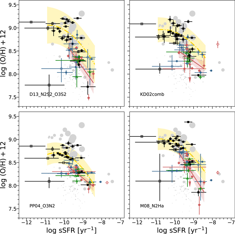
Figure 8. The sSFR vs. metallicity of the PTF SN Ic and PTF SN Ic-bl host galaxies compared to the SN–GRB hosts and local galaxies from the SDSS and LVL survey. Definitions of the symbols, lines, and color shaded areas are the same as those in Figures 4, 6, and 7. As in Figure 6, the metallicity of GRB 130702A/SN 2013dx is an upper limit, indicated by an arrow. High absolute sSFR values and low metallicities are two features present in the host samples of the SN–GRBs and PTF SNe Ic-bl. However, as gauged by a comparison with the SDSS galaxies, low metallicity is likely to be a fundamental cause for the formation of SN–GRB progenitors, whereas high sSFR is only a consequence of the low metallicity (see text).
Download figure:
Standard image High-resolution imageAs the next step, we will break the degeneracy between low metallicity and high sSFR in order to disentangle the needed conditions for the formation of SN–GRB and SN Ic-bl progenitors. In order to address this issue, we compare the hosts of SN–GRBs and PTF SNe Ic-bl with the star-forming galaxies from the SDSS on the same diagram. The two competing factors (low metallicity and high sSFR) have opposite effects on the sSFR versus metallicity relation of the SN host galaxies with respect to the same relation of the SDSS galaxies. The SDSS galaxies set the baseline for this comparison. If the sSFR versus metallicity relation of the SN host galaxies is below the same relation of the SDSS galaxies (i.e., skewed toward lower metallicities), then a low metallicity is likely the dominant effect. Otherwise, if the sSFR versus metallicity relation of the SN host galaxies is above that of the SDSS galaxies, it is likely that a high sSFR is the dominant effect.
In Figure 8, over the sSFR range in common and across all four metallicity calibrations, the sSFR versus metallicity relation of the SN–GRB hosts (red solid line) lies well below the same relation of the SDSS galaxies (yellow dashed–dotted line). This comparison demonstrates that the SN hosts are biased toward low metallicities even if we take the excess sSFR into account. In addition, if it were merely an sSFR effect such that the SN–GRB host galaxies just produced more massive stars for their galaxy mass than comparison samples like the SDSS galaxies, as suggested by Savaglio (2015), then the SN Ic hosts should also exhibit high sSFR, since SNe Ic are also explosions of massive stars, like SN–GRBs. However, this is not what we observe; rather, PTF SN Ic hosts have sSFR values lower than those of PTF SNe Ic-bl and SN–GRBs and more consistent with those of SDSS galaxies. Therefore, low metallicity is likely to be the fundamental cause for the formation of SN–GRB progenitors, whereas a high sSFR is only a consequence of the low metallicity. We note that the hosts with unreliable SFR estimates (open symbols) or metallicities as upper limits (arrows pointing to the left) are excluded from the fits.
The result of the same analysis but with the LVL galaxies as a baseline is ambiguous. The anticorrelation between sSFR and metallicity appears to be much weaker among the LVL galaxies, which may be partly due to the fact that the metallicities of the LVL galaxies are in heterogeneous calibrations.
In summary, we show that the hosts of SN–GRBs and of PTF SNe Ic-bl both exhibit high absolute sSFR values and low metallicities. In addition, we are able to break the degeneracy between the two competing factors by comparing our samples to the SDSS galaxies and to PTF SN Ic host galaxies. We find that low metallicity is likely to be the fundamental cause for the formation of SN–GRB progenitors, whereas high sSFR is only a consequence of low metallicity.
6.6. Hosts of Weird Transients and Transients with Uncertain SN Subtype
As discussed in Section 2, we consider six weird transients and transients with uncertain SN subtype, in addition to the PTF SNe Ic/Ic-bl with clean IDs. These transients are included because they are all potential SNe Ic or SNe Ic-bl, or SNe Ic with peculiar behaviors (PTF12gzk). We follow the same approach as for the PTF SNe Ic/Ic-bl with clean IDs to observe these hosts (Table 1) and to derive their host properties, including line fluxes (Table A.1), metallicities (Table 3), M* values, and SFRs (Table 4).
They are shown in all the plots as green open triangles. They do not form a unified class of SN hosts, and thus we do not summarize their distributions by CDFs or linear fits as we do for the other SN host samples. However, we note here that they generally occupy similar parameter spaces in all the plots, just as the SN–GRB and PTF SN Ic-bl hosts do: the hosts of weird transients and transients with uncertain SN subtype have overall low absolute levels of metallicity, M*, and SFR. In particular, the host of PTF12gzk is the least luminous (Ben-Ami et al. 2012) and least massive among all the SN hosts (M* = 106.95 M⊙). In terms of the 2D distributions in the M–Z (Figure 6), SFR versus M* (Figure 7), and sSFR versus metallicity (Figure 8) diagrams, the hosts of weird transients and transients with uncertain SN subtype are not outliers that significantly deviate from the average relations as defined by the SN–GRB or PTF SN Ic-bl hosts. Therefore, we do not expect qualitative changes to our analysis results on the PTF SN Ic-bl sample by including the additional SN Ic-bl candidates from these transients. Meanwhile, low-M* hosts with low SFRs and low metallicities already exist in the sample of PTF SN Ic hosts with clean IDs. We also do not expect qualitative changes to our analysis results of the PTF SN Ic sample by including a few more SN Ic candidates with similarly low M* values, SFRs, and metallicities.
In conclusion, these hosts of weird transients and transients with uncertain SN subtype exhibit similar distributions to the SN–GRB or PTF SN Ic-bl hosts in the various diagrams of host galaxy properties. They do not change our conclusions about sample comparisons.
7. Discussion: Implications for Jet Production and SN–GRB Progenitor Models
In the previous section, we found that while SN–GRBs prefer somewhat more metal-poor environments than PTF SNe Ic-bl, this preference is not statistically significant. Our finding that SN–GRBs and PTF SNe Ic-bl thus inhabit statistically similar environments could be due to the fact that indeed both types of explosions had the same low-metallicity progenitors that were able to produce a GRB—and that was not detected for the cases of SNe Ic-bl—regardless of whether those GRBs are off-axis, choked, low luminosity, missed entirely, or otherwise. Here, off-axis GRBs refer to GRBs that produced gamma-ray emission that was not observed on Earth, owing to the jet axis not being aligned with our line of sight, while their more spherical SN component was observed (though SN Ic-bl themselves, as well as CCSNe more generally, are not fully spherical; e.g., Leonard et al. 2006; Modjaz et al. 2008b; Mazzali et al. 2001). Indeed, since cosmological GRBs are highly collimated events with beaming angles of ∼10° (Frail et al. 2001; Racusin et al. 2009; Ryan et al. 2015; Zhang et al. 2015), a large number of GRBs should be viewed off-axis (though see Ryan et al. 2015 for the claim that even the GRBs are seen slightly off-axis). We discuss the evidence for whether the PTF SNe Ic-bl in our sample harbored such off-axis GRBs below, in Section 7.1.
Indeed, Mösta et al. (2015) showed that the ingredients for jet production, namely, large-scale dynamo and strong MHD turbulence, are set up in rapidly rotating stars, which would more preferably occur in low-metallicity environments via a number of different mechanisms that include binaries (e.g., Levan et al. 2016). Once the jet is produced and travels through the star, it leaves an observable imprint on the stellar envelope set into motion in the form of broad lines in the SN spectrum, indicating a significant amount of mass accelerated to high velocities. This was shown for the first time by Barnes et al. (2018), who perform an end-to-end simulation of SN–GRBs via state-of-the-art hydrodynamic and spectral synthesis simulations. Thus, broad lines would be an indicator of a central engine.
Broad lines would presumably be produced even when the jet becomes choked and does not fully reach the surface of the star; however, one may expect lower SN velocities for chocked jet engines. Indeed, Modjaz et al. (2016) showed that SNe Ic-bl without observed GRBs (including three of the PTF SNe Ic-bl in our host sample) have generally lower velocities and less broadened lines than SNe Ic-bl with GRBs but higher values and more broadening than SNe Ic. On the other hand, the spectra of SNe Ic-bl without observed GRBs may also exhibit lower velocities than those of SN–GRBs because the GRB was not pointing toward Earth. Future work that extends the pioneering research of Barnes et al. (2018) is needed to disentangle the effects of a choked jet from an off-axis GRB on the SN spectrum.
The natural implication of Barnes et al. (2018) is that the engines of SNe Ic-bl both with and without GRBs may be similar, but very different from those of their SNe Ic cousins. Indeed, we show here that PTF SNe Ic prefer environments that have statistically significant higher metallicities than SNe Ic-bl and SN–GRBs—that is, SNe Ic have environments probably not conducive for jet production. Thus, our results are in strong tension with the suggestion that all SNe Ib/c produced jets that were choked (Sobacchi et al. 2017).
While we break the degeneracy between high sSFR and low metallicity as the driver for SN Ic-bl production by favoring low metallicity (Section 6.5), it may not be the only necessary ingredient for producing SNe Ic-bl. Kelly et al. (2014) showed that a (small) sample of SNe Ic-bl from a melange of untargeted surveys and low-redshift GRBs have other host properties in common, namely, much higher SFR densities and mass densities compared to SDSS galaxies. They suggest that dense star-forming regions may be preferentially producing massive binary systems that give rise to SNe Ic-bl with and without GRBs. The SN Ic hosts in their sample seem to have more typical densities, similar to SDSS galaxies, supporting the notion that not all subtypes of stripped SNe live and die in the same environments as GRBs and thus probably did not all produce jets.
Lastly, our finding that the mass–metallicity relations as defined by SN–GRBs are not significantly different from the same relations as defined by the SDSS galaxies (in most of our considered metallicity scales and in most of our tests) contradicts earlier works based on smaller samples that used a metallicity scale that is probably not appropriate for the comparison. Thus, our finding resolves the dilemma of why SN–GRBs would have chosen a completely different galaxy population not found in the local universe of star-forming galaxies—because they do not.
7.1. Did the PTF SNe Ic-bl Harbor Off-axis GRBs?
Here we discuss whether the PTF SNe Ic-bl could have harbored off-axis GRBs. A common diagnostic for the presence of off-axis GRBs is the detection of late-time radio emission from the relativistic ejecta that have decelerated over time and are emitting more isotropically. Such an extensive radio search was conducted by Corsi et al. (2016), who observed a total of 15 broad-lined SNe Ic from PTF and iPTF, including ∼2/3 of the SNe Ic-bl in our sample (9 SNe Ic-bl out of 14 SNe Ic-bl in our sample: PTF10bzf, PTF10qts, PTF10xem, PTF10aavz, PTF11cmh, PTF11img, PTF11lbm, PTF11qcj, PTF12as) at late times with the VLA.
Corsi et al. (2016) detected radio emission from 3 out of the 15 SNe, which they cannot securely rule out as being caused by off-axis low-luminosity GRBs expanding into a constant-density ISM with nISM ≈ 10 cm−3. Two of those SNe are in our sample (PTF11cmh and PTF11qcj). Even for the nondetections, the radio limits are not deep enough to exclude on-axis GRBs similar to the radio-quiet and low-energy GRB 060218, off-axis GRBs similar to the low-energy but radio-loud GRB 980425, or high-energy off-axis GRBs such as GRB 031203 expanding into a low-density environment.
Thus, we conclude that our finding that SN–GRBs and PTF SNe Ic-bl prefer the same low-metallicity environments could be simply due to the fact that the PTF SNe Ic-bl also hosted GRBs, but whose jetted gamma-ray emission was not seen by us because of viewing-angle effects. There are two distinct possibilities of why they were not observed at radio wavelengths: (a) the GRBs were of low radio luminosity, and indeed those may be the most common kinds of GRBs (e.g., Soderberg et al. 2006), and (b) the GRBs were of high luminosity but were expanding into a low-density medium.
In addition, it is entirely possible that the PTF SNe Ic-bl are part of a continuum of engine-driven SN Ic-bl explosions that extend from the fully relativistic to the subrelativistic (Margutti et al. 2014).
8. Caveats and Future Work
8.1. Sample Bias
Samples of galaxies are biased by the survey techniques that define them, with further impact from additional selection criteria that are applied. In this section, we discuss the impacts of survey and selection biases on our conclusions, for both the SDSS and PTF SN samples.
The SDSS legacy galaxy redshift sample has an apparent r-band magnitude limit of 17.77 mag. It misses a larger fraction of galaxies with low luminosities at a higher redshift (below the yellow dashed–dotted line in Figure 3). To first order, this incompleteness is a function of M*, and thus it has mild impact on our studies of the M–Z (Figure 6) or SFR versus M* (Figure 7) relations, which are both functions of M*. Considering that metallicities are strongly correlated with M*, the impact of incompleteness on our analysis of the sSFR versus metallicity (Figure 8) is also minor. We note, however, that the incompleteness has to be taken into account in order to quantitatively address the question whether the SN–GRB hosts are unbiased tracers of the overall population of star-forming galaxies (e.g., Stanek et al. 2006; Graham & Fruchter 2013; Vergani et al. 2015).
If the sample is only affected by this magnitude limit, we can potentially correct for the incompleteness by applying a volume weight (e.g., Huang et al. 2012b). However, the volume correction only accounts for the fact that the less luminous objects are observed to be more nearby. In order to obtain valid metallicities from strong-line methods, we require a BPT class of star-forming, and thus the non-star-forming galaxies and AGNs are further eliminated. Meanwhile, the S/N cutoff in all major emission lines may result in an additional bias against metal-poor galaxies with weak [N ii] λ6584 lines. The biases with respect to the metallicity, M*, and SFR that are introduced by these selection criteria cannot be easily recovered. Therefore, our subset of SDSS galaxies only represents a population of star-forming galaxies that can reproduce the M–Z relation of Kewley & Ellison (2008) and the main star-forming sequence of Salim et al. (2007). It is not a complete sample, but it ensures a fair comparison with the previous works that usually use a similar SDSS population to the baseline of local galaxies.
Unlike the targeted SN surveys that preferentially monitor the most luminous galaxies in order to maximize the chance of SN detection, the PTF as an untargeted survey avoids such bias to massive galaxies with overall high metallicities. However, the PTF survey relies on automated detection and verification pipelines to identify all the candidates of transients (Brink et al. 2013), which may introduce a bias against transients that occur in the brightest regions of luminous galaxies. Specifically, the initial candidates are extracted from a subtraction image, which is constructed by subtracting a deep reference image of the static sky from a new image obtained nightly. The subtraction images are noisy in the brightest regions of luminous galaxies, and thus any transients there may be missed by the detection pipeline. This effect has a higher impact on the completeness of the PTF SN Ic sample, relative to the SN Ic-bl sample, owing to the fact that the PTF SNe Ic are preferentially found in the central bright regions of luminous galaxies (e.g., Anderson et al. 2015). If more SN Ic hosts with high luminosities were to be added, the difference between the SN Ic and SN Ic-bl hosts would become even more significant. Therefore, we do not expect any qualitative change to our main conclusions owing to the incompleteness of the PTF survey.
Another potential bias may have been introduced when the PTF transients were chosen for spectroscopic classification, since only a minority of PTF transients could be observed spectroscopically. However, Perley et al. (2016b) argued that in the first few years of PTF, from which our sample is drawn, any spectroscopic classification bias did not introduce a large impact on the obtained host galaxy population, since the host galaxies of PTF CCSNe (Arcavi et al. 2010) traced the general population of star-forming galaxies well. Nevertheless, any spectroscopic classification bias will be mitigated by the Zwicky Transient Facility (ZTF; Bellm 2014; Bellm & Kulkarni 2017), since they have a dedicated low-resolution prism, the SED machine (Blagorodnova et al. 2018), that is supposed to obtain spectroscopic IDs for all transients, thereby yielding bias-free samples.
8.2. Small Number Statistics and SN Bias
Compared to the effect of survey bias, our conclusion is more vulnerable to the effect of small number statistics. Although our analysis is based on the largest homogeneous samples of untargeted SNe Ic/Ic-bl from a single survey to date, as well as on all the SN–GRB hosts published recently, we still only have 14 SNe Ic-bl with clean IDs and 10 SN–GRBs in total. The power of our statistical tests is highly limited by the small sample sizes, especially for the SNe Ic-bl and SN–GRBs. In the 2D analysis, the confidence intervals of the SN–GRB relations are so broad at a fixed M* that the differences between the relations of different samples are always insignificant. Our conclusions are mostly drawn from the p-values, which only account for Type I error rates. However, the small sample sizes of the SNe Ic-bl and SN–GRBs may lead to Type II errors—that is, the tests lack power to distinguish the true small differences between the intrinsic populations.
Larger sample sizes of untargeted SNe Ic-bl and SN–GRBs are highly desired to enhance the test power. For SN–GRBs, every nearby system should be observed and published. Indeed, the host of the recent long-duration GRB 171205A may be a massive galaxy (see the GCNs by Perley & Taggart 2017 and Wang et al. 2018), though Hubble Space Telescope data are required to exclude the possibility that the GRB did not originate in a satellite galaxy of that massive galaxy, as was the case for GRB 130702A (Kelly et al. 2014). For SNe, current and upcoming surveys, such as ZTF and the Large Synoptic Survey Telescope (Ivezic et al. 2008), are expected to yield a large number of transients, which will solve this problem of small number statistics.
For our science goals, we have chosen to compare our SN hosts to hosts of GRBs that have accompanied SNe. However, there are a number of GRBs with no observed SNe (for a compilation, see, e.g., Dado & Dar 2018), with the most famous being GRB 060614 with very deep SN limits (e.g., Gal-Yam et al. 2006b)—though some of them may not be bona fide long-duration GRBs, but rather GRBs in an extended short-GRB tail (e.g., Caito et al. 2009). Those short-duration GRBs masquerading as long GRBs are not expected to be connected to CCSNe or may be altogether another type of GRB (Gehrels et al. 2006). Future work should include a complete host galaxy study of all GRBs within a certain volume, some of which do have very different host properties than those of long-duration GRBs and are more similar to those of short GRBs (e.g., Levesque & Kewley 2007 for GRB 060605).
8.3. Integrated versus IFU Studies
Ideally, we want to probe the metallicities of SN progenitor stars by measuring their metallicities from their immediate environments centered on the exact SN sites. However, our long-slit observations limit our ability to obtain such ideal measurements.
In terms of the centering accuracy, the majority of our host spectra were obtained long after the SNe themselves had faded. During observations, the exact SN sites are precisely localized by offsetting from the reference stars, and the SN sites are put at the slit centers. However, the slit-center locations are not easy to find during SN host spectrum extraction, and thus we use the positions of standard stars that are always in the slit center for guidance. Consequently, we can only localize the positions of SN sites to an accuracy that is comparable to the seeing disk. Owing to the fact that the exact SN sites are not determined, we instead try to center the aperture for spectrum extraction at the nearest Hα emission peak in the slit.
Given the above considerations and the requirement to obtain sufficiently high S/N for the spectrum, the size of the aperture for spectrum extraction corresponds to a larger physical scale than what would be ideal. By setting the aperture sizes to be twice the seeing disk, the SN sites safely fall within the apertures in most cases, and thus we name such apertures SN sites. However, rather than the metallicities at the exact SN sites, our metallicity measurements are closer to the metallicities at the nearest H ii regions, with the caveats in mind that a cluster of Hα emission may be a result of the superposition of multiple H ii regions and that the truly nearest H ii region may not be in slit. As found by the CALIFA IFS observations, the nearest H ii regions provide the best approximations of local metallicities at the exact SN sites (unbiased and with the least scatter), compared to either global metallicities or local metallicities estimated using gradients (Galbany et al. 2016).
Despite the limitations of long-slit observations, we try our best to characterize the metallicities at the SN sites by the approximations of metallicities at the nearest H ii regions. These apertures probe a typical physical scale of 2–3 kpc. They may be considered local for the SN Ic hosts that are massive, but they are indeed closer to global for the low-mass SN Ic-bl hosts. In contrast to our long-slit observations that are still integrated by nature, IFU observations with high angular resolution provide a more comprehensive way to study the very immediate environments of SN explosions.
For example, Krühler et al. (2017) present spatially resolved spectroscopy of environments obtained with MUSE throughout the host galaxy of GRB 980425/SN 1998bw. They suggest that the common strong-line calibrations using the O3N2 or N2 diagnostics lead to unrealistic variations in metallicities on subkiloparsec scales, which are likely due to the variations in ionization parameters. Using a more realistic calibration that relies on Hα, [N ii], and [S ii] (Dopita et al. 2016), those authors derive an immediate metallicity of log (O/H) + 12 ≈ 8.2 at the SN site, log (O/H) + 12 ≈ 8.3 for a galaxy-integrated spectrum, and log (O/H) + 12 ≈ 8.4 for the nearby WR region. Among the four calibrations that we choose, the D13_N2S2_O3S2 calibration should be the most comparable. For the host of GRB 980425/SN 1998bw, we obtain a metallicity of log (O/H) + 12 ≈ 8.3 in the D13_N2S2_O3S2 calibration based on data of Christensen et al. (2008), which is broadly consistent with their results.
While pioneering IFU studies have been conducted that combine high spatial resolutions, sensitivity, and broad wavelength coverage to measure the oxygen abundance of the immediate environs of different types of SNe (Kuncarayakti et al. 2013; Galbany et al. 2016; Kuncarayakti et al. 2018) and of some SN–GRBs (e.g., Christensen et al. 2008; Krühler et al. 2017), we suggest such a study for a large SN set from untargeted surveys like the one we use (PTF). Such a study would provide unarguably better constraints on the properties of SN progenitor stars. In addition, we encourage wide-field, deep studies to constrain any galaxy companions or prior mergers that may have caused the episode of star formation responsible for the SN–GRB progenitor (e.g., Izzo et al. 2017). We also suggest deeper spectra of all objects in order to measure the iron abundance from the faint emission line of [Fe iii] λ4658, since iron is the element important for stellar evolution, and since using oxygen as a tracer in young galaxies such as GRB host galaxies may overestimate the iron abundance (Hashimoto et al. 2018).
9. Conclusions
In this work, we present the largest set of host galaxy spectra of 28 SNe Ic and 14 SNe Ic-bl, all discovered by the same untargeted survey (PTF) before 2013, as well as hosts of five SN Ic/Ic-bl candidates with uncertain IDs. These spectra were taken with the Keck, Palomar, and Gemini-South telescopes. They are supplemented by SDSS spectra of the hosts of one PTF SN Ic and one PTF SN Ic-peculiar and by the broadband photometry data from SDSS, Pan-STARRS, and GALEX for all host galaxies. Taking advantage of the pyMCZ code that was developed by the SNYU group, we calculate the metallicities from the host spectra in various calibrations, including recently introduced ones. The global M*, SFR, and sSFR are derived from SED fitting to the UV to optical bands following a Bayesian approach. Combined with the emission-line fluxes and global stellar properties from the literatures for 10 SN–GRB hosts, we compare three SN host samples with each other (SN Ic vs. SN Ic-bl vs. SN–GRB) and with typical local galaxies from the SDSS and LVL, in order to uncover whether any of these SNe occur preferentially in certain types of galaxies over others, in terms of their metallicities, M* values, SFRs, and sSFR values. Such an SN host environment study provides constraints on the properties of SN progenitors that are not directly observable from the pre-explosion images for these SN types.
Compared to prior research, our study has the following strengths:
- 1.Our work is based on a homogeneous data set of the largest samples of SNe Ic and SNe Ic-bl to date that are selected from a single untargeted survey. Therefore, these host galaxies are not biased toward massive galaxies with systematically higher metallicities.
- 2.We carefully designed the strategies for observation and spectrum extraction, so that the line fluxes probe the metallicities of immediate environments of the SN explosions to the best extent allowed by our long-slit observations. In particular, most of our host spectra cover the SN sites and thus are crucial for probing the immediate environments of SN explosions, since most isolated late-type spiral galaxies display strong metallicity gradients, being more metal-rich at the center. Furthermore, the far background regions that we choose are free from the extended emission in the host galaxies, and the emission lines are corrected for stellar absorption. These measures all result in more reliable line ratios and thus metallicity measurements.
- 3.We calculate (recalculate) the gas-phase metallicities of the PTF SNe Ic/Ic-bl hosts, as well as those of SN–GRB hosts and SDSS galaxies, with the pyMCZ code, such that the metallicities of different samples can be compared for the same calibrations in a self-consistent manner. Meanwhile, we present the results in multiple calibrations to ensure that any observed trends are independent of the calibrations adopted. The four calibrations we choose (KD02, PP04, M08, and D13) include different strong-line methods, including both theoretical and hybrid ones, as well as calibrations based on several different line diagnostics (N2O2, R23, O3N2, N2, etc.). Some of them are recent calibrations and thus are not considered by previous works that compare the SN Ic-bl and GRB hosts with SDSS galaxies.
- 4.We carefully gather reliable UV to optical SEDs for the PTF SN Ic/Ic-bl hosts and apply the same methods to derive the M*, SFR, and sSFR as the MPA-JHU group does for the SDSS galaxies. In addition, if the SDSS photometry pipeline suffers significantly from shredding, we use the NS-Atlas to recover the bad pipeline photometry. We also make sure that these global values for the SN Ic/Ic-bl hosts make fair comparisons with those for the SN–GRB hosts, which we compiled from the literature. These global properties are therefore directly comparable across samples.
- 5.We identify one SN–GRB host with potential AGN contamination in a BPT diagram, as had been suggested in the literature, which may render its metallicity and SFR measurements incorrect. This has a particular impact on the statistical analysis, owing to both the very small sample size of SN–GRBs and the extreme line ratios due to AGN contamination.
- 6.We adopt rigorous analytical methods to draw quantitative results. For example, we always present the uncertainties along with the estimates for the physical parameters that are derived in this work, we apply survival analysis for upper limits, and we conduct hypothesis tests to assess the statistical significance of the observed differences in the underlying populations.
Given these improvements, we reach the following main conclusions:
- 1.As suggested by our comparisons between the distributions of line ratios, as well as of the metallicities in various calibrations (our Table 5), the three samples appear to follow the order of ZGRB ⪅ ZIc-bl < ZIc; however, the differences between the SN–GRB and SN Ic-bl hosts are not statistically significant (our Table 6), whereas those between the SN Ic-bl and SN Ic hosts are.
- 2.Given the M–Z relations, the higher metallicities of the SN Ic hosts may be explained by the fact that they are overall more massive. We isolate this effect by comparing the M–Z relations between samples. Indeed, the SN–GRBs follow an average M–Z relation that is below that for the SN Ic-bl hosts, and the average M–Z relations as defined by the SN Ic, SN Ic-bl, and SN–GRB hosts all fall slightly below the same relations as defined by the SDSS galaxies. However, none of these differences in the average relations are statistically significant at the 95% confidence level. Our result contradicts earlier works based on smaller samples that used a metallicity scale that is probably not appropriate for the comparison. Thus, our finding resolves the dilemma of why SN–GRBs would have chosen a completely different galaxy population not found in the local universe of star-forming galaxies—because they do not.
- 3.In terms of the absolute levels of global SFRs and M* values, the SN–GRB and SN Ic-bl hosts are comparable, and they are significantly below those of the SN Ic hosts. However, in terms of the relative enhancement of star formation activity as gauged by the main sequence of star formation, all three SN host samples follow similar SFR versus M* relations that are only slightly above the same relation as defined by the star-forming galaxies from SDSS.
- 4.We show that the hosts of SN–GRBs and of PTF SNe Ic-bl exhibit high absolute sSFR values and low metallicities. However, we are able to break the degeneracy between these two factors by comparing our samples to SDSS galaxies. We find that low metallicity is likely to be the fundamental cause for the formation of SN–GRB progenitors, whereas high sSFR is only a consequence of low metallicity. Thus, we resolve a major debate in the field.
Since we find that SN–GRBs and PTF SNe Ic-bl prefer statistically similar environments, in particular low metallicity, we suggest that the PTF SNe Ic-bl may have produced jets that were choked inside the star or were able to break out of the star as GRBs that were either off-axis GRBs or low-luminosity radio-quiet on-axis GRBs. Thus, broad lines in the spectra of SNe Ic may be a good indicator for the presence of a jet that either was able to break out of the star (Barnes et al. 2018) or not. However, PTF SNe Ic live and die in very different environments than both SN–GRBs and PTF SNe Ic-bl, namely, in higher-metallicity regions with lower sSFR, and may have had different progenitors than SN–GRBs and PTF SNe Ic-bl. There is no evidence supporting jet formation, in contrast to suggestions by Sobacchi et al. (2017) of all SNe Ib/c producing jets that are choked.
However, we should bear the following caveats in mind. The truly nearest H ii region to the SN site or the birth cloud of the SN progenitor star may be outside of the slit that we chose to cover both the SN site and the galaxy center, so a long-slit observation may still miss the region that is more representative of the progenitor properties. Most importantly, the strengths of our statistical tests are limited by the small sample sizes of the SN–GRBs and SNe Ic-bl. Future transient surveys that provide even larger samples of SNe Ic-bl and with homogeneous data sets of their host galaxies will help to overcome this problem of small number statistics. Future IFU studies that combine high spatial resolution, sensitivity, and broad wavelength coverage will better probe the physical conditions of the progenitor stars, and in the context of different regions across the whole galaxies. Adopting a similar analytical approach to that in the current work, such observations in the future will provide further insights into progenitor models for the formation of SNe, especially the SN–GRBs and SNe Ic-bl.
We suggest that radio searches conduct even deeper follow-up observations of SNe Ic-bl from untargeted galaxy searches in low-metallicity environments because they appear to be the best candidates for hosting off-axis GRBs, as well as extending them to later times since GRBs may stay collimated longer than was previously thought (Ryan et al. 2015).
We are grateful to Andrew MacFadyen, Brian Metzger, and Patrick Kelly for useful discussions and comments. We kindly thank S. Ben-Ami, T. G. Brink, K. I. Clubb, O. D. Fox, M. L. Graham, A. A. Miller, I. Shivvers, J. M. Silverman, and O. Yaron for co-observing at Keck and C. Ott for being the PI of some proposals submitted before 2015 September and for co-observing at Keck on 2014 November 21. M.M. and the SNYU group are supported by National Science Foundation (NSF) CAREER award AST-1352405, by NSF award AST-1413260, and by a Humboldt Faculty Fellowship. Y.-Q.L. was supported in part by an NYU GSAS Dean's Dissertation Fellowship. Support for I.A. was provided by the National Aeronautics and Space Administration (NASA) through the Einstein Fellowship Program, grant PF6-170148. A.G.-Y. is supported by the EU via ERC grant No. 725161, the Quantum universe I-Core program, the ISF, the BSF Transformative program, and a Kimmel award. Support for A.V.F.'s research group has been provided by the TABASGO Foundation, the Christopher R. Redlich Fund, and the Miller Institute for Basic Research in Science (UC Berkeley).
These results are based in part on observations obtained at the 200-inch Hale telescope, Palomar Observatory, as part of a collaborative agreement between Caltech, JPL, and Cornell University. Some of the data presented herein were obtained at the W. M. Keck Observatory, which is operated as a scientific partnership among the California Institute of Technology, the University of California, and NASA. The Observatory was made possible by the generous financial support of the W. M. Keck Foundation. The authors wish to recognize and acknowledge the very significant cultural role and reverence that the summit of Maunakea has always had within the indigenous Hawaiian community. We are most fortunate to have the opportunity to conduct observations from this mountain. Observations with the Gemini Observatory were conducted through proposals GN-2011A-Q-93 and GS-2011A-C-5 (PI Modjaz) and processed using the Gemini IRAF package. The Gemini Observatory is operated by the Association of Universities for Research in Astronomy, Inc., under a cooperative agreement with the NSF on behalf of the Gemini partnership: the NSF (United States), the National Research Council (Canada), CONICYT (Chile), Ministerio de Ciencia, Tecnología e Innovación Productiva (Argentina), and Ministério da Ciência, Tecnologia e Inovação (Brazil).
This research has made use of the GHostS database (www.grbhosts.org), which is partly funded by Spitzer/NASA grant RSA agreement No. 1287913. Furthermore, we used NASA's Astrophysics Data System Bibliographic Services (ADS) and the NASA/IPAC Extragalactic Database (NED), which is operated by the Jet Propulsion Laboratory, California Institute of Technology, under contract with NASA. This material is based on work supported by AURA through the NSF under AURA Cooperative Agreement AST-0132798 as amended.
Funding for the Sloan Digital Sky Survey IV has been provided by the Alfred P. Sloan Foundation, the U.S. Department of Energy Office of Science, and the Participating Institutions. SDSS-IV acknowledges support and resources from the Center for High-Performance Computing at the University of Utah. The SDSS website is www.sdss.org. SDSS-IV is managed by the Astrophysical Research Consortium for the Participating Institutions of the SDSS Collaboration, including the Brazilian Participation Group, the Carnegie Institution for Science, Carnegie Mellon University, the Chilean Participation Group, the French Participation Group, Harvard-Smithsonian Center for Astrophysics, Instituto de Astrofísica de Canarias, Johns Hopkins University, Kavli Institute for the Physics and Mathematics of the Universe (IPMU)/University of Tokyo, Lawrence Berkeley National Laboratory, Leibniz Institut für Astrophysik Potsdam (AIP), Max-Planck-Institut für Astronomie (MPIA Heidelberg), Max-Planck-Institut für Astrophysik (MPA Garching), Max-Planck-Institut für Extraterrestrische Physik (MPE), National Astronomical Observatories of China, New Mexico State University, New York University, University of Notre Dame, Observatário Nacional/MCTI, The Ohio State University, Pennsylvania State University, Shanghai Astronomical Observatory, United Kingdom Participation Group, Universidad Nacional Autónoma de México, University of Arizona, University of Colorado Boulder, University of Oxford, University of Portsmouth, University of Utah, University of Virginia, University of Washington, University of Wisconsin, Vanderbilt University, and Yale University.
We gratefully acknowledge NASA's support for construction, operation, and science analysis of the GALEX mission, developed in cooperation with the Centre National d'Etudes Spatiales of France and the Korean Ministry of Science and Technology.
Facilities: GALEX - Galaxy Evolution Explorer satellite, Gemini:Gillett - , Gemini:South - , Palomar:Hale - , Keck:I (LRIS) - , Keck:II (DEIMOS) - , SDSS - .
Appendix A: Tables with Emission-line Values
Here we present line-flux measurements for the full sample of 48 hosts of PTF SNe Ic/Ic-nl in Table A.1, (including 46 from new observations presented in this work and two from SDSS; see Section 3.1.4). Column (1) lists the name of the PTF SN.Column (2) indicates the type of aperture used for spectrumextraction; values other than "SNsite" indicate that the SN site is outside of the aperture (see above). Column (3) lists the emission-line redshift measured within the aperture. Because the host redshifts reported by the PTF survey are some times extracted from the host nucleus, they can be slightly different from the redshifts presented here owing to galaxy rotation. Columns (4)–(11) list flux measurements for all eight of the nebular emission lines needed to derive oxygen abundances, including [OII] λλ 3726, 3729, Hβ λ 4861, [OIII] λ 4959, [OIII] λ 5007, Hα λ 6563, [NII] λ 6584, [SII] λ 6717, and [SII] λ 6731( in units of 10−15 erg s−1 cm−2, corrected for Galactic reddeningand stellar absorption, but not for internal extinction).
Table A1. Emission-line Fluxes of PTF SN Host Galaxies in Units of 10−15 erg s−1 cm−2, Corrected for Stellar Absorption and Galactic Extinction
| PTF | Region | Redshift | [O ii] λλ3726, 3729 | Hβ λ4861 | [O iii] λ4959 | [O iii] λ5007 | Hα λ6563 | [N ii] λ6584 | [S ii] λ6717 | [S ii] λ6731 |
|---|---|---|---|---|---|---|---|---|---|---|
| Name | ||||||||||
| SN Ic-bl | ||||||||||
| 09sk | nuc | 0.036 | 16.996 ± 0.187 | 5.000 ± 0.033 | 3.762 ± 0.031 | 9.106 ± 0.057 | 15.954 ± 0.046 | 1.650 ± 0.018 | 2.903 ± 0.021 | 1.990 ± 0.020 |
| 10aavz | SNsite | 0.062 | 0.090 ± 0.004 | 0.028 ± 0.003 | 0.002 ± 0.003 | 0.031 ± 0.003 | 0.054 ± 0.004 | 0.010 ± 0.003 | 0.014 ± 0.003 | 0.010 ± 0.003 |
| 10bzf | SNsite | 0.050 | 0.116 ± 0.036 | 0.060 ± 0.005 | 0.027 ± 0.005 | 0.087 ± 0.006 | 0.153 ± 0.007 | 0.013 ± 0.005 | 0.036 ± 0.005 | 0.025 ± 0.005 |
| 10ciw | SNsite | 0.115 | 4.110 ± 0.284 | 1.046 ± 0.087 | 0.546 ± 0.077 | 2.077 ± 1.102 | 3.960 ± 0.093 | 0.703 ± 0.076 | 0.908 ± 0.054 | 0.617 ± 0.047 |
| 10qts | SNsite | 0.090 | 19.599 ± 1.018 | 8.673 ± 0.456 | 7.891 ± 0.463 | 22.479 ± 0.588 | 22.354 ± 0.702 | 0.425 ± 0.504 | 1.552 ± 0.725 | 1.341 ± 0.986 |
| 10tqv | SNsite | 0.080 | 0.089 ± 0.006 | 0.026 ± 0.002 | 0.013 ± 0.002 | 0.040 ± 0.002 | 0.075 ± 0.003 | 0.004 ± 0.002 | 0.011 ± 0.003 | 0.009 ± 0.002 |
| 10vgv | SNsite | 0.015 | 24.929 ± 2.019 | 12.483 ± 0.705 | 7.180 ± 0.673 | 22.342 ± 0.749 | 38.253 ± 1.306 | 6.204 ± 0.922 | 3.626 ± 0.900 | 2.414 ± 1.159 |
| 10xem | SNsite | 0.056 | 12.023 ± 0.093 | 10.542 ± 0.062 | 18.984 ± 0.111 | 42.328 ± 0.252 | 48.036 ± 0.062 | 1.618 ± 0.008 | 1.517 ± 0.008 | 1.263 ± 0.008 |
| 11cmh | SNsite | 0.105 | 0.164 ± 0.029 | 0.024 ± 0.006 | 0.005 ± 0.006 | 0.017 ± 0.006 | 0.068 ± 0.004 | 0.013 ± 0.006 | 0.016 ± 0.002 | 0.012 ± 0.003 |
| 11gcj | SNsite | 0.148 | 0.479 ± 0.011 | 0.130 ± 0.006 | 0.098 ± 0.005 | 0.286 ± 0.006 | 0.340 ± 0.004 | 0.028 ± 0.003 | 0.054 ± 0.006 | 0.041 ± 0.004 |
| 11img | SNsite | 0.158 | 0.135 ± 0.008 | 0.026 ± 0.006 | 0.028 ± 0.004 | 0.071 ± 0.005 | 0.141 ± 0.009 | 0.012 ± 0.004 | 0.018 ± 0.004 | 0.015 ± 0.005 |
| 11lbm | SNsite | 0.039 | 0.525 ± 0.010 | 0.169 ± 0.002 | 0.080 ± 0.002 | 0.314 ± 0.003 | 0.672 ± 0.006 | 0.039 ± 0.003 | 0.122 ± 0.004 | 0.077 ± 0.003 |
| 11qcj | SNsite | 0.028 | 5.300 ± 0.447 | 1.303 ± 0.010 | 1.120 ± 0.010 | 3.290 ± 0.018 | 3.472 ± 0.021 | 0.355 ± 0.008 | 0.617 ± 0.010 | 0.448 ± 0.009 |
| 12as | SNsite | 0.033 | 0.622 ± 0.029 | 0.133 ± 0.002 | 0.055 ± 0.001 | 0.180 ± 0.002 | 0.601 ± 0.005 | 0.089 ± 0.003 | 0.120 ± 0.004 | 0.076 ± 0.003 |
| SN Ic | ||||||||||
| 09iqd | HII3 | 0.034 | 0.341 ± 0.062 | 0.130 ± 0.005 | 0.047 ± 0.005 | 0.125 ± 0.006 | 0.590 ± 0.018 | 0.189 ± 0.014 | 0.095 ± 0.014 | 0.067 ± 0.013 |
| 10bhu | SNsite | 0.036 | 0.937 ± 0.129 | 0.284 ± 0.023 | 0.088 ± 0.024 | 0.208 ± 0.024 | 0.965 ± 0.020 | 0.228 ± 0.014 | 0.304 ± 0.017 | 0.190 ± 0.016 |
| 10fmx | SNsite | 0.044 | 0.249 ± 0.041 | 0.071 ± 0.013 | 0.026 ± 0.013 | 0.037 ± 0.014 | 0.223 ± 0.013 | 0.068 ± 0.012 | 0.049 ± 0.012 | 0.031 ± 0.011 |
| 10hfe | SNsite | 0.048 | 3.633 ± 0.270 | 0.991 ± 0.018 | 0.282 ± 0.014 | 0.716 ± 0.018 | 2.419 ± 0.024 | 0.697 ± 0.013 | 0.627 ± 0.013 | 0.463 ± 0.012 |
| 10hie | SNsite | 0.067 | 0.299 ± 0.036 | 0.103 ± 0.013 | 0.075 ± 0.014 | 0.241 ± 0.019 | 0.268 ± 0.010 | 0.005 ± 0.006 | 0.040 ± 0.008 | 0.043 ± 0.009 |
| 10lbo | SNsite | 0.052 | 0.529 ± 0.036 | 0.183 ± 0.017 | 0.013 ± 0.017 | 0.117 ± 0.018 | 0.501 ± 0.021 | 0.138 ± 0.018 | 0.135 ± 0.016 | 0.075 ± 0.015 |
| 10ood | SNsite | 0.060 | 1.353 ± 0.132 | 0.502 ± 0.011 | 0.427 ± 0.011 | 1.190 ± 0.017 | 1.769 ± 0.020 | 0.186 ± 0.010 | 0.217 ± 0.010 | 0.166 ± 0.010 |
| 10osn | HII | 0.038 | 0.168 ± 0.201 | 0.104 ± 0.007 | 0.018 ± 0.007 | 0.050 ± 0.009 | 0.584 ± 0.013 | 0.220 ± 0.010 | 0.093 ± 0.009 | 0.067 ± 0.008 |
| 10qqd | SNsite | 0.080 | 0.032 ± 0.031 | 0.071 ± 0.011 | ⋯ | ⋯ | 0.867 ± 0.021 | 0.187 ± 0.014 | 0.145 ± 0.015 | 0.095 ± 0.018 |
| 10tqi | HII2 | 0.038 | 0.940 ± 0.015 | 0.374 ± 0.003 | 0.078 ± 0.002 | 0.285 ± 0.003 | 1.229 ± 0.007 | 0.285 ± 0.005 | 0.280 ± 0.005 | 0.183 ± 0.004 |
| 10wal | SNsite | 0.028 | 0.124 ± 0.010 | 0.055 ± 0.002 | 0.005 ± 0.002 | 0.025 ± 0.002 | 0.177 ± 0.004 | 0.046 ± 0.003 | 0.052 ± 0.004 | 0.033 ± 0.005 |
| 10xik | SNsite | 0.071 | 0.187 ± 0.011 | 0.063 ± 0.002 | 0.032 ± 0.002 | 0.130 ± 0.002 | 0.164 ± 0.004 | 0.014 ± 0.003 | 0.031 ± 0.003 | 0.015 ± 0.003 |
| 10yow | HII1 | 0.025 | 0.063 ± 0.029 | 0.241 ± 0.021 | ⋯ | ⋯ | 1.287 ± 0.022 | 0.385 ± 0.014 | 0.096 ± 0.014 | 0.105 ± 0.015 |
| 10ysd | SNsite | 0.096 | 0.555 ± 0.128 | 0.667 ± 0.017 | 0.032 ± 0.015 | 0.107 ± 0.017 | 2.377 ± 0.021 | 1.025 ± 0.013 | 0.413 ± 0.012 | 0.301 ± 0.011 |
| 10zcn | SNsite | 0.021 | 0.233 ± 0.110 | 0.192 ± 0.008 | 0.014 ± 0.007 | 0.029 ± 0.007 | 0.826 ± 0.014 | 0.270 ± 0.010 | 0.164 ± 0.009 | 0.090 ± 0.011 |
| 11bov | SNsite | 0.022 | 1.035 ± 0.050 | 0.270 ± 0.006 | 0.238 ± 0.006 | 0.660 ± 0.009 | 0.659 ± 0.006 | 0.066 ± 0.003 | 0.166 ± 0.004 | 0.083 ± 0.003 |
| 11hyg | SNsite | 0.029 | 0.158 ± 0.038 | 0.200 ± 0.008 | 0.017 ± 0.007 | 0.050 ± 0.007 | 1.136 ± 0.014 | 0.459 ± 0.010 | 0.184 ± 0.010 | 0.123 ± 0.011 |
| 11ixk | SNsite | 0.024 | 0.451 ± 0.194 | 0.161 ± 0.016 | 0.003 ± 0.014 | 0.087 ± 0.015 | 0.475 ± 0.013 | 0.176 ± 0.011 | 0.114 ± 0.011 | 0.107 ± 0.011 |
| 11jgj | SNsite | 0.040 | 0.319 ± 0.115 | 0.173 ± 0.015 | 0.034 ± 0.013 | 0.045 ± 0.014 | 1.005 ± 0.016 | 0.340 ± 0.010 | 0.162 ± 0.011 | 0.139 ± 0.011 |
| 11klg | HII2 | 0.026 | 0.115 ± 0.007 | 0.109 ± 0.002 | 0.011 ± 0.002 | 0.019 ± 0.002 | 0.393 ± 0.006 | 0.159 ± 0.003 | 0.088 ± 0.004 | 0.057 ± 0.003 |
| 11rka | SNsite | 0.074 | 89.090 ± 1.447 | 57.711 ± 0.601 | 64.998 ± 0.653 | 179.874 ± 1.029 | 180.433 ± 1.291 | 3.248 ± 0.550 | 13.202 ± 0.602 | 8.788 ± 0.647 |
| 12cjy | SNsite | 0.044 | 0.452 ± 0.030 | 0.359 ± 0.011 | 0.015 ± 0.009 | 0.033 ± 0.010 | 1.161 ± 0.012 | 0.407 ± 0.008 | 0.238 ± 0.008 | 0.160 ± 0.007 |
| 12dcp | SNsite | 0.031 | 6.228 ± 0.112 | 1.788 ± 0.037 | 0.780 ± 0.021 | 2.233 ± 0.045 | 6.878 ± 0.034 | 1.497 ± 0.014 | 1.090 ± 0.013 | 0.802 ± 0.012 |
| 12dtf | SNsite | 0.062 | 0.884 ± 0.052 | 0.348 ± 0.009 | 0.302 ± 0.009 | 0.962 ± 0.015 | 1.609 ± 0.013 | 0.156 ± 0.007 | 0.192 ± 0.008 | 0.142 ± 0.007 |
| 12fgw | SNsite | 0.055 | 2.597 ± 0.074 | 1.602 ± 0.019 | 0.248 ± 0.015 | 0.742 ± 0.018 | 8.329 ± 0.029 | 2.454 ± 0.013 | 1.309 ± 0.011 | 0.891 ± 0.010 |
| 12hvv | nuc | 0.029 | 0.705 ± 0.328 | 0.172 ± 0.019 | 0.034 ± 0.019 | 0.100 ± 0.019 | 0.498 ± 0.015 | 0.136 ± 0.012 | 0.173 ± 0.015 | 0.087 ± 0.012 |
| 12jxd | SNsite | 0.025 | 0.854 ± 0.017 | 0.504 ± 0.004 | 0.139 ± 0.003 | 0.240 ± 0.003 | 2.353 ± 0.010 | 0.805 ± 0.006 | 0.527 ± 0.006 | 0.349 ± 0.006 |
| 12ktu | SNsite | 0.031 | 0.292 ± 0.109 | 0.406 ± 0.010 | 0.025 ± 0.008 | 0.054 ± 0.008 | 1.648 ± 0.016 | 0.567 ± 0.011 | 0.229 ± 0.011 | 0.177 ± 0.011 |
| Weird/Uncertain SN Subtype | ||||||||||
| 09ps | SNsite | 0.107 | 0.757 ± 0.047 | 0.244 ± 0.019 | 0.162 ± 0.023 | 0.329 ± 0.034 | 0.930 ± 0.016 | 0.083 ± 0.011 | 0.169 ± 0.010 | 0.120 ± 0.009 |
| 10bip | nuc | 0.051 | ⋯ | 0.135 ± 0.008 | 0.171 ± 0.009 | 0.409 ± 0.010 | 0.636 ± 0.008 | 0.078 ± 0.006 | 0.115 ± 0.005 | 0.100 ± 0.005 |
| 10gvb | SNsite | 0.098 | 0.205 ± 0.083 | 0.074 ± 0.004 | 0.082 ± 0.005 | 0.274 ± 0.007 | 0.293 ± 0.006 | 0.011 ± 0.004 | 0.039 ± 0.006 | 0.022 ± 0.005 |
| 10svt | SNsite | 0.031 | 1.188 ± 0.037 | 0.546 ± 0.009 | 0.459 ± 0.009 | 1.303 ± 0.015 | 1.613 ± 0.019 | 0.096 ± 0.011 | 0.172 ± 0.015 | 0.116 ± 0.013 |
| 12gzk | SNsite | 0.148 | ⋯ | 0.750 ± 0.016 | 0.645 ± 0.015 | 1.928 ± 0.022 | 2.322 ± 0.020 | 0.051 ± 0.006 | 0.125 ± 0.007 | 0.091 ± 0.007 |
| 12hni | SNsite | 0.106 | ⋯ | 1.012 ± 0.023 | 1.246 ± 0.018 | 3.639 ± 0.031 | 3.170 ± 0.029 | 0.266 ± 0.010 | 0.370 ± 0.011 | 0.312 ± 0.011 |
Appendix B: Notes on Individual SN–GRBs
In Table B1 we present the emission line values of the SN-GRB hosts discussed in Section 4.1, along with their nebular emission-line fluxes that we adopt in order to compute their line ratios and metallicities with the same calibrations as we use for the PTF SN hosts (see Section 5.1). As we explain below for each object in detail, if multiple sets of flux measurements exist in the literature, we adopt the ones providing flux uncertainties, since the code we are using requires flux uncertainties for computing metallicity uncertainties (see Section 5.1). If multiple spectra are extracted from the same host at different sites, we include only the one from the SN site. Here follow some individual notes for all SN–GRBs discussed in Section 4.1.
- 1.GRB 980425/SN 1998bw.—We adopt the host line fluxes presented by Christensen et al. (2008) because they are based on IFU observations and are detected at the SN site. However, neither the [O iii] λ4959 line flux nor its flux uncertainty is reported therein. We assume the [O iii] λ4959 flux to be one-third that of [O iii] λ5007 and the flux uncertainties to be at the 10% level.
- 2.XRF 020903, GRB 030329/SN 2003dh, and GRB/XRF 060218/SN 2006aj.—For these three SN–GRB hosts we use the host line fluxes from Han et al. (2010), who reanalyze archival Very Large Telescope (VLT) spectra of GRB host galaxies. Being a systematic study of multiple sources, Han et al. (2010) correct for stellar absorption by modeling the continuum and stellar absorption lines, as we do for the PTF SN hosts.
- 3.GRB 031203/SN 2003lw.—We use the host line fluxes averaged from four VLT observations in Margutti et al. (2007). Because this source is very close to the Galactic plane, the far-infrared map from Schlegel et al. (1998) is unreliable along our line of sight toward this galaxy. In order to correct for Galactic extinction, we follow Margutti et al. (2007) and assume E(B − V)MW = 0.72 mag.
- 4.GRB 100316D/SN 2010bh.—We use line fluxes from Izzo et al. (2017), which are extracted at the SN site from IFU observations and have been corrected for stellar absorption in the host galaxy and extinction due to the Milky Way. We note that if we use the line ratios of Levesque et al. (2011), who neither correct for stellar absorption nor provide uncertainties, then we compute a lower metallicity for this host than when using the values from Izzo et al. (2017).
- 5.GRB 120422A/SN 2012bz.—We adopt the line fluxes measured by Schulze et al. (2014) for the galaxy center rather than for the explosion site because fewer emission lines of interest are detected at the explosion site, including the Hβ line that is only marginally detected at the explosion site. According to Schulze et al. (2014), a slightly higher metallicity is derived at the explosion site (log (O/H) + 12 ≳ 8.57 ± 0.05) than for the galaxy center (log (O/H) + 12 = 8.43 ± 0.01), in the PP04_N2Hα calibration (Pettini & Pagel 2004). Therefore, with our choice of galaxy center spectrum over SN site spectrum, we are likely to slightly underestimate the metallicity of the immediate SN–GRB environment in this case.
- 6.GRB 130427A/SN 2013cq.—Xu et al. (2013) report the final metallicity values in a specific calibration, but not the emission-line fluxes on which that value is based. We requested the original spectra from the authors and measured the line fluxes via IRAF's splot.
- 7.GRB 130702A/SN 2013dx.—We note that this is the first GRB host galaxy that has been recognized as the satellite dwarf galaxy of a more massive, metal-rich galaxy (Kelly et al. 2013). The [N ii] flux for its host galaxy is an upper limit in Kelly et al. (2013), and the [O iii] lines are unavailable, so we can only obtain upper limits on metallicities in the KD02comb (N2 based in this case) and M08_N2Hα calibrations (see Section 5.1).
- 8.GRB 161219B/SN 2016jca.—Ashall et al. (2017) report the final metallicity range of the host galaxy for various calibrations, but not the emission-line fluxes on which that range is based. We requested the emission-line fluxes from the authors. The fluxes for the host galaxy of this most recent event are from an afterglow spectrum. We adopt the M* and SFR values for this host from Cano et al. (2017b). Note that the emission-line fluxes are also available in Cano et al. (2017b), which result in line ratios that are consistent with the values that we adopt. However, the Hβ line is unavailable in Cano et al. (2017b), which is important for extinction estimation.
Table B1. SN–GRB Host Galaxy Emission-line Fluxes, in Units of 10−17 erg s−1 cm−2, Corrected for Galactic Extinction
| SN–GRB Name | z | [O ii] λλ3726, 3729 | Hβ λ4861 | [O iii] λ4959 | [O iii] λ5007 | Hα λ6563 | [N ii] λ6584 | [S ii] λ6717 | [S ii] λ6731 |
|---|---|---|---|---|---|---|---|---|---|
| GRB 980425/SN 1998bwa | 0.00867 | 260.7 ± 26.07 | 75.5 ± 7.55 | 60.9 ± 6.09 | 182.7 ± 18.27 | 449.4 ± 44.94 | 50.3 ± 5.03 | 91.9 ± 9.19 | 68.4 ± 6.84 |
| XRF 020903b | 0.2506 | 11.48 ± 0.36 | 8.58 ± 0.29 | 15.56 ± 0.31 | 44.11 ± 0.33 | 26.03 ± 0.21 | 0.77 ± 0.1 | 2.14 ± 0.17 | 1.28 ± 0.09 |
| GRB 030329/SN 2003dhc | 0.16867 | 19.62 ± 0.32 | 9.8 ± 0.16 | 11.74 ± 0.2 | 30.53 ± 0.26 | 30.94 ± 0.27 | 0.29 ± 0.15 | 3.82 ± 0.09 | 1.89 ± 0.08 |
| GRB 031203/SN 2003lwd | 0.10536 | 529.54 ± 34.22 | 624.65 ± 40.06 | 1391.93 ± 88.99 | 4200.29 ± 268.59 | 2517.63 ± 188.04 | 130.84 ± 9.71 | 86.14 ± 5.53 | 68.28 ± 4.37 |
| GRB/XRF 060218/SN 2006aje | 0.03342 | 224.25 ± 1.01 | 91.43 ± 0.65 | 108.4 ± 0.48 | 291.23 ± 0.66 | 261.51 ± 0.54 | 10.73 ± 0.32 | 15.4 ± 0.36 | 11.56 ± 0.41 |
| GRB 100316D/SN 2010bhf | 0.0592 | ⋯ | 6.542 ± 0.142 | 6.688 ± 0.148 | 19.268 ± 0.203 | 22.785 ± 0.208 | 2.15 ± 0.108 | 3.097 ± 0.115 | 2.42 ± 0.109 |
| GRB120422A/SN 2012bzg | 0.28253 | 58.0 ± 6.7 | 12.8 ± 0.4 | 8.3 ± 0.3 | 25.1 ± 0.5 | 53.6 ± 0.5 | 8.1 ± 0.4 | 9.1 ± 0.2 | 6.7 ± 0.3 |
| GRB 130427A/SN 2013cqh | 0.3399 | 18.55 ± 1.33 | 5.401 ± 0.384 | 4.21 ± 0.448 | 9.766 ± 0.756 | 18.76 ± 0.705 | 3.189 ± 0.583 | 3.477 ± 1.403 | 7.689 ± 2.078 |
| GRB 130702A/SN 2013dxi | 0.145 | ⋯ | 4.3 ± 0.52 | ⋯ | ⋯ | 11.10 ± 0.05 | 0.54 | ⋯ | ⋯ |
| GRB 161219B/SN 2016jcaj | 0.1475k | 8.31 ± 0.38 | 2.58 ± 0.29 | 1.6 ± 0.28 | 3.99 ± 0.47 | 5.59 ± 0.18 | 0.41 ± 0.12 | ⋯ | ⋯ |
Notes.
aChristensen et al. (2008), for the SN region. We assume that the flux uncertainties are at the 10% level and that the line flux for [O iii] λ4959 is one-third of that for [O iii] λ5007. bHan et al. (2010), who correct for stellar absorption. cHan et al. (2010), who correct for stellar absorption. dMargutti et al. (2007), line fluxes averaged from four VLT observations. eHan et al. (2010), who correct for stellar absorption. fIzzo et al. (2017), who correct for extinction and stellar absorption. gSchulze et al. (2014), at the host center site. hSpectrum from Xu et al. (2013), and we remeasured the line fluxes via splot in IRAF. iKelly et al. (2013). Note that their [N ii] flux is a 2σ upper limit. jAshall et al. (2017). kCano et al. (2017a).Download table as: ASCIITypeset image
Owing to our limited access to raw spectra, we are not able to run platefit on this sample of SN–GRB host galaxies to correct for stellar absorption. The only SN–GRB hosts for which stellar absorption has been removed are from Han et al. (2010) (XRF 020903, GRB 030329/SN 2003dh, and GRB/XRF 060218/SN 2006aj) and from Izzo et al. (2017) (GRB 100316D/SN 2010bh). We note that the stellar absorption correction is mostly ignored in the other SN–GRB works. However, the GRB hosts are generally known to be vigorously star-forming, so that stellar absorption is expected to be minimal.
Appendix C: More Details about the Metallicity Calibrations and Scales We Adopt in This Paper
- 1.The KD02comb calibration is theoretical. It automatically chooses the optimal calibration from KD02_N2O2 (Kewley & Dopita 2002), KK04_N2Hα, and KK04_R23 (Kobulnicky & Kewley 2004), given the input line fluxes, and is implemented by pyMCZ following Appendices 2.2 and 2.3 from Kewley & Ellison (2008). The N2O2 ratio is not influenced by the diffuse ionized gas (Zhang et al. 2016) and is not sensitive to the ionization parameter (q), defined as the number of hydrogen-ionizing photons passing through a unit area per second, divided by the hydrogen density of the gas. Moreover, the N2O2 ratio is a strong monotonic function of the metallicity at log([N ii]/[O ii]) > −1.2 (Kewley & Dopita 2002). For log([N ii]/[O ii]) > −1.2, or log (O/H) + 12 ≳ 8.4, the KD02comb calibration chooses KD02_N2O2, if the desired line fluxes are available. For log([N ii]/[O ii]) < −1.2, or log (O/H) + 12 < 8.4, the KD02comb calibration uses an average of the KK04_R23 lower branch and the M91_R23 lower branch. The relation between oxygen abundance and R23 is double valued, but the parameter q can break the degeneracy. To calculate the R23-based metallicities, pyMCZ follows the recommendation of Kewley & Ellison (2008) to derive a consistent q and metallicity solution via an iterative approach. Note that the sample of 500 SDSS galaxies reveals a mild effect of discontinuity in the metallicity distribution around log(O/H) + 12 ≈ 8.4 in the KD02comb calibration. A similar gap is more evident in the KD02 calibration, originally introduced by Kewley & Dopita (2002). This discontinuity may be caused by the S/N cutoff in line detections that are applied on the SDSS sample. We discuss the impact of this effect in Section 6.2.
- 2.The D13_N2S2_O3S2 calibration is theoretical. It is the only calibration out of the four that relies on the [S ii] λ6717 and [S ii] λ6731 lines. This calibration is calculated by the Python module pyqz (version 0.4, the first publicly released version), following the MAPPINGS IV simulations (Dopita et al. 2013). In particular, the photoionization models used by Kewley & Dopita (2002) and by Kewley et al. (2004) are updated by including new atomic data within a modified photoionization code and by assuming a more realistic κ distribution for the energy of the electrons in the H ii regions, rather than the simple Maxwell–Boltzmann distribution assumed in prior works.
- 3.The PP04_O3N2 calibration is hybrid. It is a linear calibration with O3N2 (Pettini & Pagel 2004). This calibration is included mostly for comparison reasons, because it is commonly used in the literature investigating SN and GRB environments (see Modjaz et al. 2011, and references therein). We note that the PP04 calibrations are superseded by the M13 ones (Marino et al. 2013), including another O3N2-based calibration, M13_O3N2. Working with empirical calibrations, Marino et al. (2013) find a significantly shallower slope in the relationship between the N2 and O3N2 ratios and the metallicity. We confirmed by our PTF SN hosts that the M13_N2 and M13_O3N2 calibrations give systematically lower metallicities for more metal-rich systems, relative to all the other theoretical or hybrid calibrations that we have presented here. As expected, purely empirical calibrations give lower metallicity values. However, the M13_O3N2 calibration is calibrated over −1 < log [([O iii] λ5007/Hβ)/([N ii] λ6584/Hα)] < 1.7. This calibration is only valid for half of the SN–GRB hosts. To avoid the problem of small number statistics, it is critical to use a calibration that is valid for more SN–GRB hosts, and thus we choose the PP04_O3N2 calibration over M13_O3N2.
- 4.The M08_N2Hα calibration relies on only two lines with small separation in wavelength, Hα and N2, and thus is available for all of the host galaxies of PTF SNe and SN–GRBs. The employed [N ii] λ6584 line saturates at high metallicities, and thus usually the N2-based calibrations saturate in high-metallicity galaxies, at log(O/H) + 12 ≳ 8.8 (Kewley & Ellison 2008). As a hybrid calibration, M08_N2Hα in particular is Te based at low metallicities but uses KD02 photoionization models at high metallicities, and thus it is less affected by such saturation. However, the sample of 500 SDSS galaxies reveals a clear discontinuity in the metallicity distribution around log(O/H) + 12 ≈ 9.2 in the M08_N2Hα calibration. To derive a smooth M–Z relation, we eliminate the SDSS galaxies with log(O/H) + 12 > 9.2 in the M08_N2Hα calibration. Note that among all the PTF SN Ic/Ic-bl and SN–GRB hosts, only one SN Ic host has log(O/H) + 12 > 9.2 in the M08_N2Hα calibration and thus is affected by the discontinuity.
Appendix D: Comparison with Literature Values for All Samples
In order to perform a self-consistent analysis, we have calculated metallicities for the SDSS galaxies and the host galaxies of all the PTF SNe Ic/Ic-bl and SN–GRBs in our sample using the same approach and code. Here, we compare our metallicity values with the literature values for the same galaxies for all our samples (PTF SNe, SN–GRBs, and SDSS).
- 1.SDSS galaxies.—For the SDSS galaxies, we can reproduce the Kewley & Ellison (2008) M–Z relation with the metallicities in the PP04_O3N2 calibration that we have in common.
- 2.PTF host galaxies.—For the hosts of PTF SNe Ic/Ic-bl, we compare our values with those of Valenti et al. (2012) for PTFbov/SN 2011bm and those of Sanders et al. (2012) for seven PTF Ic/Ic-bl hosts. In summary, their values are in excellent agreement with our results, with ours being superior since we either have higher-S/N data, provide detailed error bars, or have better IDs for the SNe.Valenti et al. (2012) obtain line fluxes from the "vicinity" of PTFbov/SN 2011bm and calculate a metallicity in the PP04_O3N2 scale that is consistent with our value (though they do not provide error bars). Sanders et al. (2012) present seven PTF SN Ic/Ic-bl hosts in their sample, including PTF10bzf (SN Ic-bl), which is listed as SN 2010ah by Sanders et al. (2012). However, there have been changes in the IDs of some of the PTF SNe owing to our improved SN identification (see Section 2): PTF09q is listed as an SN Ic by Sanders et al. (2012), but we reclassify it as an SN Ia and thus eliminate it from this work; PTF10bip and PTF10vgv are classified as SNe Ic by Sanders et al. (2012), but we update the ID of PTF10bip to be of uncertain SN type and PTF10vgv to be an SN Ic-bl, as shown by Modjaz et al. (2016). In conclusion, there are three SNe Ic-bl, two SNe Ic, and one SN with an uncertain type in common between our and their samples of the PTF SNe Ibc, according to our improved IDs. Among them, the host of PTF10aavz (SN Ic-bl) has weak emission-line detections that are not sufficient to estimate the metallicities in Sanders et al. (2012), whereas we have obtained the metallicities for this host based on our spectroscopic observations. Among the six different metallicity calibrations that are considered by Sanders et al. (2012), there are two for which we overlap (KD02comb and PP04_O3N2). In Sanders et al. (2012), the metallicity in the KD02comb calibration is only reported for PTF11hyg, and the metallicity in the PP04_O3N2 calibration is reported for PTF10bzf, PTF10bip, and PTF11hyg. Only three out of the five SN hosts that we have in common can be compared in the same calibrations. Their values are in excellent agreement with ours within 1σ, except for PTF11hyg in PP04_O3N2. The line ratios for the host of PTF11hyg are measured at the SN site, which is not coincident with the nucleus, but suggest an ionization source from an AGN according to the BPT diagram (see Section 6.1). Though an off-nuclear AGN-like spectrum is possible, our own line fluxes suggest an ionization source from star formation at the SN site, and we adopt them as being more reliable. In short, our metallicities agree with those of Sanders et al. (2012) in almost all cases; in the one case where they do not, we think that our data are superior.
- 3.Host galaxies of SN–GRBs.—For the host galaxies of SN–GRBs, we compare our metallicities with those derived in the same papers from which we collected the line fluxes. Based on the same input of line fluxes, the metallicity results are generally in agreement within the uncertainties for the same calibrations, as expected. We note that the metallicities from the literature have no uncertainties reported for GRB 130702A/SN 2013dx (Kelly et al. 2013, upper limit) and GRB 161219B/SN 2016jca (Ashall et al. 2017). If the exact same calibration used in the literature is not calculated by pyMCZ, we choose the one that is based on the same line ratios. For example, line fluxes for three of the following SN–GRB hosts are drawn from Han et al. (2010), who reanalyze all archival VLT data of nearby GRB host galaxies (z < 1), including those of SN–GRBs XRF 020903, GRB 030329/SN 2003dh, and GRB/XRF 060218/SN 2006aj. Those authors report the metallicities in the K99 calibration (Kobulnicky et al. 1999), which is an R23-based one. These three hosts have low metallicities and low N2O2 ratios, so that their pyMCZ-derived metallicities for the KD02comb calibration are also R23 based. We therefore compare the literature values in the KK99 scale from Han et al. (2010) with the metallicities that we compute in the KD02comb calibration and find excellent agreement for all three hosts. The only exception with a large discrepancy comes from the comparison for GRB 031203/SN 2003lw, which may be due to AGN contamination (see Section 6.1). Note that Margutti et al. (2007) and Han et al. (2010) derived different line ratios for this host from almost the same observational data (Han et al. 2010 uses additional archival VLT data from 2005 that Margutti et al. 2007 do not show). The Han et al. (2010) values are less reliable in this case (X. Han and F. Hammer 2019, private communication), so we adopt the line fluxes from Margutti et al. (2007) for GRB 031203/SN 2003lw. Margutti et al. (2007) report a Te-based metallicity of log(O/H) + 12 = 8.12 ± 0.04, and Han et al. (2010) report one of 8.11 ± 0.11 in the K99 calibration. Similarly, pyMCZ yields a low metallicity in both the PP04_O3N2 and M08_N2Hα calibrations but a high metallicity in the KD02comb calibration: log(O/H) + 12 =
 . It is outside the grid of Dopita et al. (2013), so the value in the D13_N2S2_O3S2 calibration is not calculated. This source has a high N2O2 ratio with log([N ii]/[O ii]) > −1.2. Without additional information from the auroral [O iii] λ4363 line, pyMCZ places it on the upper branch of R23, and its metallicity value for the KD02comb calibration is based on the N2O2 diagnostic. The host spectra of GRB 031203/SN 2003lw most likely have a contribution from AGN activity. The effect of an AGN contribution is small for the N2O2-based calibrations but larger for the calibrations using [O iii] as a diagnostic (e.g., Kewley et al. 2004; Kewley & Ellison 2008). We therefore keep its N2O2-based metallicity in the KD02comb calibration, which is much higher than our O3N2-based value or the R23-based and Te-based values from the literature. As mentioned in Section 6.1, we present our analysis results with and without this object in order to assess its impact, and we plot it with a different symbol in our plots.

Appendix E: Identifying AGNs from the BPT Diagram
Usually all relevant lines are required to be detected with S/N > 3 to place the source on a BPT diagram, but we include sources with detected lines even at S/N < 3 in Figure 4, in order to not introduce systematic bias (see Section 5.1). However, there are three hosts with nondetections in certain lines such that they are excluded from the diagram. Two of them are SN Ic hosts (PTF10qqd and PTF10yow), with nondetections in [O iii] λ5007. The third is an SN–GRB host (GRB 130702A/SN 2013dx), with a nondetection in [O iii] λ5007 and only an upper limit in [N ii] λ6584. Following the classification scheme proposed by Brinchmann et al. (2004), they all have [N ii] λ6584/Hα < 0.6, so we can rule out the possibility of them being low-S/N AGNs. In addition, these three hosts have Hα lines detected at S/N > 2, so we can further classify them as low-S/N star-forming galaxies.
All the other host galaxies in our PTF SN and SN–GRB samples are shown in the bottom left panel of Figure 4, and all of them lie below the solid division; they are not classified as AGNs, but rather as star-forming galaxies. Another similar diagram is constructed by, for example, Kewley et al. (2001), which depends on the same emission lines except that the [N ii] λ6584 line is substituted with the [S ii] λλ6717, 6731 lines.
Thus, the strong-line methods that we adopt for the metallicity calculations are valid, and so are the Hα-based SFRs for SN–GRB hosts in particular. All of the hosts form a clean sequence on the diagram. As a sanity check, there is no apparent scatter of host galaxies off this sequence, which would have otherwise rendered the line flux measurements suspicious.
We examine whether these classifications are robust against the effects of extinction. In general, the BPT diagram is designed to be less affected by extinction, since it depends on two line ratios, each involving two lines with small separation in wavelengths. We use line fluxes from Table A.1 (for PTF SNe Ic/Ic-bl, weird transients, and transients with uncertain SN subtype) and Table 4 (for SN–GRBs) to make the plots, which are corrected for Galactic extinction but not for internal extinction. Applying extinction correction has the effect of shifting a data point downward and to the left in a BPT diagram, though always by a small amount. With the extra corrections for internal extinction, all the data points are expected to move even farther away from the divisions, making no changes to their classifications. However, if the Galactic extinction correction is not applied, all the data points are expected to move slightly toward the division, which again makes no change to their classifications, except for the host of GRB 031203/SN 2003lw.
The host of GRB 031203/SN 2003lw appears as a moderate outlier above the main distribution but sits just below the two divisions in Figure 4—that is, still in the regime of star-forming galaxy. It will shift into the regime of AGN-powered objects if its line fluxes are not corrected for Galactic extinction. Note that GRB 031203/SN 2003lw happens to lie very close to the Galactic plane, and thus the Galactic extinction is both large and highly uncertain. We follow Margutti et al. (2007) to assume E(B − V)MW = 0.72 mag, which results in its current location in Figure 4. With its data point sitting near the divisions and the error bars crossing them, plus large and highly uncertain Galactic extinction, this host has a classification that is highly uncertain. Based on several diagnostics, Levesque et al. (2010a) conclude that it shows definitive evidence of AGN activity and cannot be classified as a purely star-forming galaxy. On the contrary, Margutti et al. (2007) and Prochaska et al. (2004) both classify it as star-forming but did not account for the considerable error bars.
Thus, for the host of GRB 031203/SN 2003lw, the metallicities derived from strong-line methods in Section 5.1 should be taken as approximate, with the same caveat applying to their SFRs, which are based on Hα. Accordingly, we denote them by open diamonds in all plots to indicate that their metallicity and SFR estimates are less reliable. For the hypothesis tests on metallicity distributions (see Section 6.2), we present p-values in both cases, with and without it in the SN–GRB sample.
For the host galaxy sample of PTF SNe Ic and SNe Ic-bl we do not detect any AGN emission. However, we note that for a majority of our PTF sample our spectra do not probe the very center of the host galaxy where an AGN would reside. Studies that do probe the center of the SN host galaxies, such as the CALIFA survey, do find that a high fraction of SN hosts founded in a variety of targeted galaxies harbor AGNs (22% of the SN Ibc hosts; Galbany et al. 2018).
Appendix F
In Table F1 we list input SDSS and GALEX photometry of the 48 PTF host galaxies, which we use for our SED fitting as described in Section 5.2, as well as the output values for the computed stellar masses and SFRs. We report the output values as the median values of the full PDFs, along with the uncertainties denoting the 16th and 84th percentiles from the distributions.
Table F1. SED Fitting of PTF SN Ic and PTF SN Ic-bl Hosts: Input Photometry and Output Parameters
| PTF | u | g | r | i | z | FUV | NUV | log M* | log SFR |
|---|---|---|---|---|---|---|---|---|---|
| Name | (mag) | (mag) | (mag) | (mag) | (mag) | (mag) | (mag) | (M⊙) | (M⊙ yr−1) |
| SN Ic-bl | |||||||||
| 09sk | 18.741 ± 0.033 | 17.811 ± 0.008 | 17.522 ± 0.007 | 17.301 ± 0.01 | 17.134 ± 0.021 | 19.596 ± 0.151 | 19.127 ± 0.08 |

|

|
| 10aavz | 20.827 ± 0.157 | 19.575 ± 0.026 | 19.056 ± 0.022 | 18.892 ± 0.029 | 18.588 ± 0.071 | 21.68 ± 0.186 | 21.089 ± 0.12 |

|

|
| 10bzf/SN10ah | 20.111 ± 0.11 | 19.382 ± 0.024 | 19.019 ± 0.025 | 18.701 ± 0.032 | 18.574 ± 0.091 | 21.631 ± 0.317 | 21.637 ± 0.197 |

|

|
| 10ciw | 20.669 ± 0.122 | 19.651 ± 0.024 | 19.187 ± 0.024 | 18.884 ± 0.026 | 18.808 ± 0.071 | 21.387 ± 0.412 | 21.301 ± 0.317 |

|

|
| 10qts | 22.562 ± 0.372 | 21.884 ± 0.079 | 21.509 ± 0.086 | 22.162 ± 0.208 | 21.208 ± 0.394 | 21.846 ± 0.493 | 21.215 ± 0.433 |

|

|
| 10tqv | 23.212 ± 0.799 | 21.686 ± 0.103 | 21.085 ± 0.084 | 20.926 ± 0.121 | 20.498 ± 0.305 | ⋯ | ⋯ |

|

|
| 10vgv | 16.293 ± 0.015 | 15.278 ± 0.003 | 14.755 ± 0.003 | 14.498 ± 0.003 | 14.34 ± 0.008 | 17.845 ± 0.025 | 16.81 ± 0.014 |

|

|
| 10xem | 18.547 ± 0.025 | 17.761 ± 0.007 | 18.359 ± 0.012 | 17.861 ± 0.011 | 18.346 ± 0.055 | 19.298 ± 0.042 | 19.056 ± 0.028 |

|

|
| 11cmh | 21.054 ± 0.271 | 20.022 ± 0.044 | 19.572 ± 0.047 | 19.356 ± 0.07 | 19.575 ± 0.333 | ⋯ | ⋯ |

|

|
| 11gcj | 21.197 ± 0.148 | 20.386 ± 0.036 | 19.979 ± 0.034 | 19.842 ± 0.048 | 19.906 ± 0.188 | 21.047 ± 0.034 | 20.913 ± 0.016 |

|

|
| 11img | 23.858 ± 1.67 | 21.817 ± 0.148 | 22.275 ± 0.294 | 21.74 ± 0.28 | 21.852 ± 0.964 | ⋯ | ⋯ |

|

|
| 11lbm | 19.306 ± 0.082 | 18.121 ± 0.011 | 17.751 ± 0.014 | 17.599 ± 0.018 | 17.505 ± 0.061 | 20.44 ± 0.156 | 20.455 ± 0.182 |

|

|
| 11qcj | 17.256 ± 0.014 | 16.616 ± 0.004 | 16.531 ± 0.005 | 16.457 ± 0.007 | 16.522 ± 0.079 | 17.953 ± 0.022 | 17.71 ± 0.009 |

|

|
| 12as | 17.617 ± 0.02 | 16.665 ± 0.004 | 16.312 ± 0.004 | 16.11 ± 0.005 | 15.964 ± 0.014 | 18.481 ± 0.011 | 18.072 ± 0.007 |

|

|
| SN Ic | |||||||||
| 09iqd | ⋯ | 15.043 ± 0.01 | 14.45 ± 0.092 | 14.037 ± 0.01 | 13.872 ± 0.01 | ⋯ | ⋯ |

|

|
| 10bhu | 18.086 ± 0.03 | 16.971 ± 0.006 | 16.554 ± 0.005 | 16.339 ± 0.007 | 16.123 ± 0.016 | 19.278 ± 0.106 | 18.874 ± 0.063 |

|

|
| 10fmx | 17.016 ± 0.019 | 15.287 ± 0.003 | 14.488 ± 0.002 | 14.108 ± 0.002 | 13.794 ± 0.005 | 18.598 ± 0.097 | 17.688 ± 0.048 |

|

|
| 10hfe | 16.134 ± 0.024 | 15.436 ± 0.003 | 15.22 ± 0.004 | 15.01 ± 0.005 | 14.924 ± 0.012 | 16.633 ± 0.008 | 16.228 ± 0.003 |

|

|
| 10hie | 19.968 ± 0.135 | 18.448 ± 0.016 | 18.092 ± 0.018 | 17.873 ± 0.021 | 18.015 ± 0.091 | ⋯ | ⋯ |

|

|
| 10lbo | 19.534 ± 0.075 | 18.417 ± 0.015 | 17.914 ± 0.013 | 17.635 ± 0.017 | 17.469 ± 0.051 | 20.817 ± 0.198 | 20.443 ± 0.084 |

|

|
| 10ood | 18.991 ± 0.075 | 17.875 ± 0.011 | 17.691 ± 0.012 | 17.457 ± 0.013 | 17.498 ± 0.043 | 19.896 ± 0.054 | 19.474 ± 0.027 |

|

|
| 10osn | 15.971 ± 0.023 | 14.712 ± 0.003 | 13.997 ± 0.002 | 13.708 ± 0.002 | 13.452 ± 0.005 | 17.946 ± 0.058 | 17.165 ± 0.027 |

|

|
| 10qqd | 18.68 ± 0.061 | 17.481 ± 0.009 | 16.924 ± 0.008 | 16.598 ± 0.008 | 16.422 ± 0.025 | ⋯ | ⋯ |

|

|
| 10tqi | 16.495 ± 0.013 | 15.418 ± 0.002 | 15.016 ± 0.008 | 14.745 ± 0.003 | 14.585 ± 0.007 | 17.265 ± 0.04 | 16.854 ± 0.024 |

|

|
| 10wal | 16.436 ± 0.023 | 15.15 ± 0.003 | 14.525 ± 0.004 | 14.224 ± 0.004 | 13.977 ± 0.008 | 17.704 ± 0.061 | 17.2 ± 0.036 |

|

|
| 10xik | ⋯ | 18.851 ± 0.1 | 18.554 ± 0.084 | 18.396 ± 0.052 | 18.377 ± 0.04 | 20.934 ± 0.365 | 20.415 ± 0.265 |

|

|
| 10yow | 14.688 ± 0.011 | 13.175 ± 0.001 | 12.381 ± 0.001 | 11.961 ± 0.001 | 11.685 ± 0.002 | 17.108 ± 0.054 | 16.159 ± 0.026 |

|

|
| 10ysd | 18.945 ± 0.037 | 17.701 ± 0.007 | 17.107 ± 0.006 | 16.706 ± 0.006 | 16.464 ± 0.013 | 21.479 ± 0.341 | 20.332 ± 0.135 |

|

|
| 10zcn | 15.403 ± 0.015 | 14.255 ± 0.002 | 13.743 ± 0.005 | 13.419 ± 0.003 | 13.199 ± 0.005 | 17.372 ± 0.055 | 16.602 ± 0.026 |

|

|
| 11bov/SN11bm | 15.931 ± 0.009 | 15.078 ± 0.002 | 14.79 ± 0.002 | 14.644 ± 0.002 | 14.559 ± 0.008 | 16.628 ± 0.013 | 16.353 ± 0.003 |

|

|
| 11hyg/SN11ee | 14.163 ± 0.005 | 12.994 ± 0.001 | 12.604 ± 0.001 | 12.285 ± 0.001 | 12.023 ± 0.002 | 15.817 ± 0.009 | 15.335 ± 0.005 |

|

|
| 11ixk | 15.983 ± 0.01 | 14.581 ± 0.002 | 13.924 ± 0.001 | 13.567 ± 0.002 | 13.276 ± 0.004 | 17.165 ± 0.017 | 16.614 ± 0.007 |

|

|
| 11jgj | 17.291 ± 0.026 | 15.624 ± 0.003 | 14.77 ± 0.003 | 14.326 ± 0.003 | 13.936 ± 0.005 | ⋯ | ⋯ |

|

|
| 11klg | 16.123 ± 0.042 | 14.319 ± 0.001 | 13.564 ± 0.001 | 13.098 ± 0.001 | 12.884 ± 0.008 | ⋯ | ⋯ |

|

|
| 11rka | 21.649 ± 0.199 | 21.201 ± 0.058 | 21.126 ± 0.078 | 20.831 ± 0.092 | 20.722 ± 0.268 | 21.755 ± 0.496 | 22.247 ± 0.402 |

|

|
| 12cjy | 17.341 ± 0.024 | 16.132 ± 0.003 | 15.546 ± 0.004 | 15.222 ± 0.003 | 14.974 ± 0.01 | 19.011 ± 0.108 | 18.287 ± 0.046 |

|

|
| 12dcp | 15.708 ± 0.035 | 14.458 ± 0.002 | 13.912 ± 0.002 | 13.622 ± 0.002 | 13.411 ± 0.006 | ⋯ | ⋯ |

|

|
| 12dtf | 21.047 ± 0.096 | 19.942 ± 0.018 | 19.72 ± 0.02 | 19.298 ± 0.021 | 19.332 ± 0.066 | ⋯ | ⋯ |

|

|
| 12fgw | 17.602 ± 0.016 | 16.398 ± 0.004 | 15.838 ± 0.003 | 15.433 ± 0.003 | 15.211 ± 0.008 | 19.097 ± 0.116 | 18.562 ± 0.06 |

|

|
| 12hvv | 18.454 ± 0.046 | 17.333 ± 0.007 | 16.809 ± 0.007 | 16.545 ± 0.008 | 16.416 ± 0.024 | 19.688 ± 0.055 | 19.288 ± 0.037 |

|

|
| 12jxd | 15.241 ± 0.011 | 13.995 ± 0.001 | 13.324 ± 0.001 | 12.947 ± 0.001 | 12.633 ± 0.002 | 16.358 ± 0.024 | 15.926 ± 0.014 |

|

|
| 12ktu | ⋯ | 13.121 ± 0.012 | 12.528 ± 0.015 | 12.242 ± 0.003 | 12.01 ± 0.004 | 16.223 ± 0.037 | 15.647 ± 0.019 |

|

|
| Weird/Uncertain SN Subtype | |||||||||
| 09ps | 20.749 ± 0.112 | 19.773 ± 0.019 | 19.482 ± 0.02 | 19.194 ± 0.021 | 19.203 ± 0.085 | ⋯ | ⋯ |

|

|
| 10bip | 20.024 ± 0.074 | 18.835 ± 0.012 | 18.591 ± 0.013 | 18.372 ± 0.015 | 18.293 ± 0.05 | 20.998 ± 0.21 | 20.52 ± 0.109 |

|

|
| 10gvb | 21.131 ± 0.202 | 20.125 ± 0.041 | 19.883 ± 0.05 | 19.519 ± 0.051 | 19.884 ± 0.308 | 21.477 ± 0.44 | 21.289 ± 0.308 |

|

|
| 10svt | ⋯ | 18.302 ± 0.063 | 18.002 ± 0.05 | 17.958 ± 0.051 | 17.809 ± 0.085 | ⋯ | ⋯ |

|

|
| 12gzk | 18.958 ± 0.194 | 18.782 ± 0.015 | 18.804 ± 0.018 | 18.86 ± 0.03 | 18.61 ± 0.075 | 19.341 ± 0.022 | 19.409 ± 0.005 |

|

|
| 12hni | 19.685 ± 0.102 | 18.961 ± 0.018 | 18.624 ± 0.02 | 18.391 ± 0.023 | 18.386 ± 0.09 | 20.203 ± 0.31 | 19.939 ± 0.178 |

|

|
Footnotes
- 18
Note the caveat that this SN Ic-bl rate is based on only one object in the LOSS sample.
- 19
- 20
PTF09q (Ic
Ia), PTF10bip (Ic uncertain: Ic/Ic-bl), PTF10vgv (Ic Ic-bl); see also Modjaz et al. (2016). - 21
- 22
- 23
- 24
- 25
- 26
We acknowledge that we are running multiple tests on the same data, which may cause one to find statistical significance when there is none owing to data dredging (i.e., just by chance) if the threshold is not adjusted accordingly. But since we instead find a null result in each case, we are not concerned about this being an issue here.
- 27
Optimal non-bipartite matching algorithms perform naively as O(N4), though they can be optimized to O(N3); e.g., Papadimitriou & Steiglitz (1982).


