


Abstract
Based on the early-year observations from Neil Gehrels Swift Observatory, Liang et al. performed a systematic analysis for the shallow decay component of gamma-ray bursts (GRBs) X-ray afterglow, in order to explore its physical origin. Here we revisit the analysis with an updated sample (with Swift/XRT GRBs between 2004 February and 2017 July). We find that with a larger sample, (1) the distributions of the characteristic properties of the shallow decay phase (e.g., tb, SX, ΓX,1, and αX,1) still accord with normal or lognormal distribution; (2) ΓX,1 and Γγ still show no correlation, but the tentative correlations of durations, energy fluences, and isotropic energies between the gamma-ray and X-ray phases still exist; (3) for most GRBs, there is no significant spectral evolution between the shallow decay segment and its follow-up segment, and the latter is usually consistent with the external-shock models; (4) assuming that the central engine has a power-law luminosity release history as  , we find that the value q is mainly distributed between −0.5 and 0.5, with an average value of 0.16 ± 0.12; (5) the tentative correlation between
  and
and  disappears, so that the global three-parameter correlation (
 ) becomes less significant; (6) the anticorrelation between LX and
  and the three-parameter correlation (
 ) indeed exist with a high confidence level. Overall, our results are generally consistent with Liang et al., confirming their suggestion that the shallow decay segment in most bursts is consistent with an external forward shock origin, probably due to a continuous energy injection from a long-lived central engine.
Export citation and abstract BibTeX RIS
1. Introduction
Gamma-ray bursts (GRBs) are considered to be the most extreme explosive events in the universe, which contains two phenomenological emission phases: the prompt phase (with an initial prompt  -ray emission) and the afterglow phase (with a longer-lived broadband emission) (Zhang 2019). Although there are many uncertainties in the detailed physics of the prompt emission, mainly due to our poor understanding of the degree of magnetization of the GRB jet (Zhang 2014; Kumar & Zhang 2015), a generic synchrotron external-shock model has been constructed for interpreting the broadband afterglow data (Rees & Meszaros 1992, 1994; Meszaros & Rees 1993; Mészáros & Rees 1997; Gao et al. 2013; Wang et al. 2015).
In the pre-Swift era, the simple external-shock signal was found to successfully explain a bunch of late-time afterglow data (Waxman 1997; Wijers et al. 1997; Huang et al. 1999, 2000; Wijers & Galama 1999; Panaitescu & Kumar 2001, 2002; Yost et al. 2003). With the successful launch of the Neil Gehrels Swift Observatory, unprecedented new information about early-time afterglows was revealed (Burrows et al. 2005b; Tagliaferri et al. 2005; Nousek et al. 2006; O'Brien et al. 2006; Zhang et al. 2006; Evans et al. 2009), especially in the X-ray band, thanks mainly to the rapid slewing and precise localization capability of its onboard X-ray Telescope (XRT; Burrows et al. 2005a). After 6 months of data accumulating, a five-segment canonical X-ray afterglow light curve was proposed (Zhang et al. 2006), including a distinct rapidly decaying component, a shallow decay component, a normal decay component, a post jet break component and X-ray flares. With two years of data (with ∼100 GRBs), a series of systematic analysis of the Swift XRT data was performed, in order to explore the physical origin for each segment of the canonical light curve (Liang et al. 2007, 2008; Willingale et al. 2007; Zhang et al. 2007b; Evans et al. 2009).
After 14 years of operation, thousands of Swift GRBs were detected by XRT, it is of great interest to revisit the early analysis and see whether the previous results are still consistent with the larger sample. In this work, we focus on the analysis of the shallow decay component from Liang et al. (2007; hereafter L07). L07 made a comprehensive analysis of the properties of the shallow decay segment with a sample of 53 long Swift GRBs detected before 2007 February. Their statistic results are summarized as follows: (1) the distributions of shallow decay segment parameters are normal and lognormal, with  ,
,  ,
,  , and
, and  (2) The spectrum of the shallow decay phase is softer than that of the prompt gamma-ray phase, while the X-ray fluence and isotropic energy are almost linearly correlated with gamma-ray fluence and gamma-ray energy, respectively; (3) there is no significant spectral evolution between the shallow decay segment and its follow-up segment, and the follow-up segment in most bursts is consistent with the closure relations of external-shock models; (4) within the scenario of refreshed external shocks, the average energy injection index q ∼ 0, suggesting a roughly constant injection luminosity from the central engine; (5) there is an empirical multivariate relation between parameters
  (henceforth the prime marks properties in the burst rest frame). Based on these results, L07 proposed that the shallow decay segment in most bursts is consistent with an external forward shock origin with continuous energy injection from a long-lived central engine. For a small fraction of bursts, whose post-break phases significantly deviate from the external-shock models, the shallow decay phase might be of internal origin and demand a long-lived emission component directly from the central engine.
In this work, we revisit the results of L07 with Swift-observed GRBs between 2004 February and 2017 July. In addition, it has been discovered that there exists a rough anticorrelation between the rest frame X-ray plateau end time ( ) and X-ray luminosity LX (Dainotti et al. 2008, 2010, 2011a). The slope is roughly −1 (Dainotti et al. 2013b). This suggests that the total plateau energy has relatively small scatter: a longer plateau tends to have a lower luminosity and vice versa. Dainotti et al. (2011b) analyzed and suggested correlations between LX with several prompt emission parameters, including the isotropic energy
  . Xu & Huang (2012) claimed that a three-parameters collection, expressed as
  , becomes tighter. On the other hand, Dainotti et al. (2016, 2017) extend the
  correlation by adding a third parameter (the peak luminosity in the prompt emission
  ), and find that the new
  correlation becomes much tighter, which is 37% tighter than the Xu & Huang (2012) correlation. In this work, we also test these relations based on our new sample.
2. Data Reduction and Sample Selection
The XRT light curve data were downloaded from the Swift/XRT team website5 (Belokurov et al. 2009), and processed with HEASOFT v6.12. 1291 Swift GRBs were detected by Swift/XRT between 2004 February and 2017 July, with 625 GRBs having well-sampled XRT light curves, which contain at least six data points, excluding upper limits. We then fit the XRT light curves (in logarithmic scale) with the multisegment broken power-law (BPL) function. Here the multivariate adaptive regression spline (MARS) technique (e.g., Friedman 1991) is adopted, which can automatically determine both variable selection and functional form, resulting in an explanatory predictive model. It has been proven that MARS can automatically fit the XRT light curve with the multisegment BPL function (results are consistent with fitting results provided by the XRT GRB online catalog), detect and optimize all breaks, and record all break times and power-law indices for each segment (see Zhang et al. 2014 and Gao et al. 2017 for details). We find that the distribution of the index difference between adjacent segments for all GRBs could be fitted with a Gaussian function (with mean value 0.6 and standard deviation 0.3). To avoid the potential overfitting problem from the MARS technique, we treat the adjacent segments with index difference smaller than 0.3 as one component when calculating the segment time span.
We define segments with decay slopes shallower than 0.8 and time spans in log scale larger than 0.4 dex6 as the shallow decay component candidates. 284 GRBs are excluded due to the lack of any shallow decay candidates. Among the rest of the 341 GRBs, 67 bursts are further excluded because there are too few data points or there seem to be weak flare signatures in the shallow decay segments. Moreover, we excluded 54 GRBs whose shallow decay candidate segments lack a follow-up segment; namely, the shallow decay segment is the only segment, or the last segment, in the light curve. 18 GRBs are excluded because they consist of more than one nonadjacent shallow decay candidate, which will be discussed in a separate work. GRB 060218 is excluded because its early shallow decay behavior in the X-ray light curve should be mainly determined by the shock break-out emission instead of external-shock emission (Campana et al. 2006).
For the remaining 201 GRBs, we record the beginning time (t1) of the shallow decay segment and the end time (t2) of its follow-up segment. We then fit the light curve in the time interval [t1, t2] with a smoothed BPL function
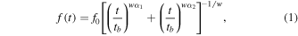
with  and
and  representing the decay scopes of the pre-break segment and the post-break segment, and w determining the sharpness of the break. Here we adopt w = 3 as suggested in L07, in order to make a better comparison with their results. All fitting light curves are shown in Figure 1, and the best fitting parameters are collected in Table 1. The X-ray fluence (SX) of the shallow decay segment is obtained by integrating the fitted light curve from t1 to tb. Note that here we further exclude three bursts in our sample because the difference between their
  and
and  are smaller than 0.3.

Figure 1.
XRT light curves for the bursts in our sample. The solid red lines are the best fits with a smooth broken power law for the shallow decay phase and its follow-up decay phase. All the component figures are available in the figure set. (The complete figure set (198 images) is available.)
Download figure:
Standard image High-resolution imageTable 1. Part I: XRT Observations and Fitting Results for Our Sample
| GRB Name |
 a
a
|
 a
a
|
 b
b
|
αX,1b | αX,2b |
 b
b
|
SXc | ΓX,1d | ΓX,2d |
|---|---|---|---|---|---|---|---|---|---|
| (s) | (s) | (s) | ( ) ) |
||||||
| 050319 | 2.61 | 6.32 | 4.52 | 0.5 ± 0.03 | 1.54 ± 0.11 | 96.98/91 | 3.1 ± 0.46 |

|

|
| 050401 | 2.1 | 5.91 | 3.67 | 0.55 ± 0.02 | 1.43 ± 0.04 | 429.9/317 | 6.51 ± 0.8 | 1.91 ± 0.04 |

|
| 050416A | 2.26 | 6.77 | 3.22 | 0.39 ± 0.1 | 0.9 ± 0.02 | 111.4/91 | 0.31 ± 0.15 |

|

|
| 050505 | 3.5 | 6.2 | 4.31 | 0.68 ± 0.07 | 1.65 ± 0.06 | 233.1/188 | 2.32 ± 0.57 |

|

|
| 050607 | 2.84 | 6.21 | 3.99 | 0.57 ± 0.1 | 1.17 ± 0.08 | 19.9/20 | 0.15 ± 0.11 |

|

|
| 050712 | 3.68 | 6.19 | 4.82 | 0.65 ± 0.07 | 1.3 ± 0.1 | 75.22/41 | 0.74 ± 0.47 |

|

|
| 050713A | 2.41 | 6.23 | 3.99 | 0.58 ± 0.03 | 1.29 ± 0.03 | 97.41/79 | 2.43 ± 0.64 |

|

|
| 050713B | 3.06 | 6.14 | 4.04 | −0.2 ± 0.1 | 1.02 ± 0.03 | 151/107 | 1.72 ± 0.22 |

|
1.83 ± 0.13 |
| 050714B | 3.75 | 5.89 | 4.56 | 0.22 ± 0.29 | 0.85 | 17.6/11 | 0.1 ± 0.05 |

|

|
| 050802 | 2.89 | 6.08 | 3.72 | 0.48 ± 0.07 | 1.56 ± 0.02 | 208.4/143 | 2.18 ± 0.31 |

|
1.88 ± 0.08 |
| 050803 | 3.5 | 6.2 | 4.04 | −0.46 ± 0.13 | 1.57 ± 0.02 | 307.2/104 | 1.51 ± 0.14 | 1.8 ± 0.14 | 2.07 ± 0.11 |
| 050814 | 3.82 | 5.96 | 4.95 | 0.67 ± 0.05 | 2.08 ± 0.16 | 44.62/40 | 0.76 ± 0.15 | 1.98 ± 0.16 |

|
| 050822 | 3.02 | 6.66 | 4.27 | 0.29 ± 0.07 | 1.08 ± 0.03 | 131.8/91 |

|

|

|
| 050824 | 3.75 | 6.41 | 4.82 | 0.24 ± 0.1 | 0.93 ± 0.08 | 67.98/37 | 0.67 ± 0.34 |

|

|
| 050826 | 4.03 | 5.1 | 4.61 | 0.27 ± 0.33 | 1.96 ± 0.71 | 1.045/5 | 0.12 ± 0.06 |

|

|
| 050915B | 2.86 | 5.97 | 5.03 | 0.46 ± 0.04 | 1.6 ± 0.28 | 10.68/14 | 0.53 ± 0.19 |

|

|
| 050922B | 3.22 | 6.37 | 5.31 | 0.35 ± 0.05 | 1.53 ± 0.12 | 36.68/16 | 1.65 ± 10.43 |

|

|
| 051109B | 2.51 | 5.2 | 3.5 | 0.24 ± 0.13 | 1.28 ± 0.07 | 21.88/19 | 0.13 ± 0.04 |

|

|
| 051221A | 2.86 | 6.03 | 4.63 | 0.56 ± 0.04 | 1.43 ± 0.07 | 92.32/55 | 0.66 ± 0.15 | 1.91 ± 0.15 |

|
| 060108 | 2.66 | 5.57 | 4.11 | 0.26 ± 0.06 | 1.25 ± 0.08 | 46.49/25 | 0.36 ± 0.1 |

|

|
| 060109 | 2.8 | 5.57 | 3.79 | −0.08 ± 0.07 | 1.49 ± 0.05 | 66.51/48 | 0.44 ± 0.05 |

|

|
| 060115 | 2.9 | 5.62 | 4.5 | 0.62 ± 0.05 | 1.2 ± 0.12 | 39.9/23 | 0.48 ± 0.28 |

|

|
| 060203 | 3.5 | 5. 59 | 4.46 | 0.77 ± 0.15 | 1.49 ± 0.22 | 55.94/34 | 0.08 ± 0.7 |

|

|
| 060204B | 2.63 | 5. 8 | 3.9 | 0.63 ± 0.06 | 1.52 ± 0.05 | 79.3/59 | 1.23 ± 0.27 | 2.03 ± 0.11 |

|
| 060219 | 2.35 | 5.75 | 4.35 | 0.51 ± 0.05 | 1.35 ± 0.11 | 13.94/14 | 0.19 ± 0.08 |

|

|
| 060306 | 2.57 | 5.58 | 3.51 | 0.31 ± 0.14 | 1.06 ± 0.03 | 94.32/76 | 0.58 ± 0.33 |

|
2.1 ± 0.13 |
| 060312 | 2.39 | 5.46 | 4.37 | 0.72 ± 0.07 | 1.56 ± 0.46 | 54.06/21 | 0.5 ± 0.37 |

|

|
| 060413 | 3.07 | 5.3 | 4.41 | 0.17 ± 0.05 | 3.03 ± 0.1 | 393.1/145 | 7.16 ± 0.55 |

|

|
| 060428A | 2.15 | 6.52 | 4.98 | 0.53 ± 0.02 | 1.37 ± 0.05 | 170/141 | 6.48 ± 1.15 |

|

|
| 060502A | 2.35 | 6.2 | 4.57 | 0.59 ± 0.03 | 1.18 ± 0.05 | 64.41/62 | 2.22 ± 0.67 | 1.89 ± 0.13 |

|
| 060510A | 2.14 | 5.76 | 3.77 | 0.09 ± 0.05 | 1.5 ± 0.02 | 196.2/158 |

|

|

|
| 060604 | 3.56 | 6.2 | 4.32 | 0.39 ± 0.09 | 1.29 ± 0.06 | 98.72/66 | 0.51 ± 0.14 |

|

|
| 060605 | 2.24 | 5.25 | 3.92 | 0.42 ± 0.03 | 2.06 ± 0.08 | 85.71/74 | 1.22 ± 0.1 |

|

|
| 060607A | 2.68 | 5 | 4.11 | 0.44 ± 0.02 | 3.58 ± 0.08 | 253.9/173 | 12.01 ± 0.71 |

|
1.56 ± 0.08 |
| 060614 | 3.66 | 6.4 | 4.69 | 0.09 ± 0.04 | 1.94 ± 0.04 | 181/150 |

|

|

|
| 060707 | 2.58 | 6.53 | 5.09 | 0.62 ± 0.03 | 1.32 ± 0.12 | 59.43/33 | 1.91 ± 0.88 |

|

|
| 060712 | 2.55 | 6 | 3.97 | 0.34 ± 0.08 | 1.13 ± 0.05 | 23.93/22 | 0.17 ± 0.06 |

|

|
| 060714 | 2.47 | 6.11 | 3.67 | 0.38 ± 0.09 | 1.27 ± 0.04 | 81.86/47 | 0.88 ± 0.27 |

|

|
| 060719 | 2.71 | 5.88 | 3.87 | 0.48 ± 0.07 | 1.25 ± 0.04 | 60.03/50 | 0.55 ± 0.17 |

|

|
| 060729 | 2.83 | 7.1 | 4.8 | 0.12 ± 0.02 | 1.37 ± 0.01 | 1011/706 | 10.69 ± 0.38 | 1;96 ± 0.05 | 1.97 ± 0.05 |
| 060804 | 2.16 | 5.41 | 2.9 | −0.31 ± 0.16 | 1.17 ± 0.06 | 38.76/28 | 0.5 ± 0.12 |

|

|
| 060805A | 2.16 | 5.46 | 3.56 | 0.19 ± 0.17 | 1.5 ± 0.1 | 15.69/8 | 0.09 ± 0.03 |

|

|
| 060807 | 2.43 | 5.7 | 3.88 | 0.001 ± 0.04 | 1.64 ± 0.04 | 169.6/92 | 1.13 ± 0.08 | 1.9 ± 0.12 |

|
| 060813 | 2 | 5.5 | 3.24 | 0.6 ± 0.03 | 1.3 ± 0.02 | 333/234 | 4.08 ± 0.75 | 1.83 ± 0.08 | 1.78 ± 0.09 |
| 060814 | 3.15 | 6.12 | 4.1 | 0.44 ± 0.08 | 1.36 ± 0.03 | 272.1/161 | 1.96 ± 0.34 | 1.97 ± 0.12 | 2.08 ± 0.09 |
| 060906 | 2.8 | 5.41 | 4.05 | 0.24 ± 0.06 | 1.74 ± 0.09 | 66.64/32 | 0.39 ± 0.05 |

|

|
| 060908 | 1.8 | 5.94 | 2.84 | 0.56 ± 0.07 | 1.44 ± 0.04 | 62.81/33 | 0.86 ± 0.23 |

|

|
| 060923C | 2.88 | 6.08 | 5.32 | 0.54 ± 0.06 | 1.85 ± 0.29 | 14.88/16 | 1.11 ± 0.38 |

|

|
| Part II: XRT Observations and Fitting Results for Our Sample | |||||||||
| 060927 | 1.82 | 5 | 3.79 | 0.76 ± 0.05 | 2.49 ± 0.81 | 5.479/13 | 0.45 ± 0.16 |

|

|
| 061004 | 2.72 | 5.28 | 4.19 | 0.68 ± 0.07 | 1.64 ± 0.29 | 24.67/17 | 0.4 ± 0.24 |

|

|
| 061019 | 3.4 | 5.86 | 5.07 | 0.81 ± 0.05 | 1.96 ± 0.39 | 80.89/42 | 1.46 ± 0.73 |

|

|
| 061121 | 2.37 | 6.32 | 3.71 | 0.36 ± 0.03 | 1.4 ± 0.02 | 369.5/269 | 7.04 ± 0.84 |

|
1.79 ± 0.06 |
| 061201 | 1.9 | 5.08 | 3.44 | 0.54 ± 0.07 | 2.05 ± 0.11 | 33.23/23 | 1.39 ± 0.27 |

|

|
| 061202 | 2.94 | 5.78 | 4.22 | −0.1 ± 0.05 | 1.73 ± 0.03 | 202.2/116 | 2.55 ± 0.15 |

|

|
| 061222A | 2.33 | 6.19 | 4.68 | 0.73 ± 0.01 | 1.72 ± 0.03 | 516.3/327 | 12.37 ± 0.89 | 1.84 ± 0.06 | 2.05 ± 0.1 |
| 070103 | 2.2 | 5.13 | 3.16 | −0.23 ± 0.14 | 1.42 ± 0.06 | 31.95/24 | 0.21 ± 0.04 |

|

|
| 070110 | 3.5 | 4.5 | 4.31 | 0.066 ± 0.05 | 9.05 ± 0.52 | 111.1/107 | 2.45 ± 0.13 | 2.04 ± 0.08 |

|
| 070129 | 3.15 | 6.21 | 4.25 | 0.15 ± 0.08 | 1.14 ± 0.03 | 102.4/80 | 0.62 ± 0.12 | 2.21 ± 0.16 |

|
| 070306 | 2.73 | 6.05 | 4.48 | 0.11 ± 0.03 | 1.81 ± 0.04 | 193.4/140 | 5.24 ± 0.34 | 1.8 ± 0.09 |

|
| 070328 | 2.18 | 5.92 | 2.84 | 0.25 ± 0.03 | 1.46 ± 0.01 | 683.4/531 | 5.57 ± 0.35 | 2.09 ± 0.04 | 1.9 ± 0.07 |
| 070420 | 2.51 | 5.72 | 3.51 | 0.23 ± 0.07 | 1.37 ± 0.02 | 230/139 | 2.53 ± 0.32 |

|

|
| 070429A | 3.33 | 6.05 | 5.69 | 0.36 ± 0.08 | 3.03 ± 0.5 | 34.6/12 | 0.92 ± 0.14 |

|

|
| 070508 | 1.83 | 5.9 | 2.46 | 0.18 ± 0.32 | 0.95 ± 0.18 | 611/484 | 0.15 ± 0.55 | 1.8 ± 0.06 | 1.76 ± 0.04 |
| 070529 | 2.31 | 5.78 | 3.02 | 0.48 ± 0.16 | 1.25 ± 0.04 | 38.09/30 | 0.42 ± 0.17 |

|

|
| 070621 | 2.60 | 5.90 | 3.47 | 0.68 ± 0.19 | 1.14 ± 0.06 | 31.29/25 | 0.18 ± 0.83 |

|

|
| 070628 | 2 | 4.91 | 3.93 | 0.44 ± 0.02 | 1.29 ± 0.03 | 301.4/192 | 4.12 ± 0.26 | 1.9 ± 0.13 | 2.01 ± 0.11 |
| 070809 | 2.74 | 4.82 | 3.78 | −0.06 ± 0.19 | 1.30 ± 0.15 | 16.71/11 | 0.16 ± 0.07 |

|

|
| 070810A | 2.1 | 4.54 | 3.14 | 0.36 ± 0.25 | 1.32 ± 0.06 | 46.44/31 | 0.37 ± 0.24 |

|

|
| 071118 | 2.99 | 5.06 | 4.11 | 0.59 ± 0.06 | 2.18 ± 0.13 | 83.57/60 | 2.52 ± 0.4 | 1.36 ± 0.11 |

|
| 080320 | 3 | 6.32 | 4.85 | 0.60 ± 0.04 | 1.25 ± 0.06 | 131/96 | 2.03 ± 0.6 | 1.97 ± 0.11 |

|
| 080328 | 2.4 | 4.7 | 3.08 | 0.43 ± 0.09 | 1.19 ± 0.03 | 235.6/155 | 2.33 ± 0.64 | 1.72 ± 0.16 |

|
| 080409 | 2.16 | 5.03 | 3.27 | −0.01 ± 0.14 | 1.3 ± 0.14 | 15.24/8 | 0.14 ± 0.04 |

|

|
| 080413B | 2.1 | 5.24 | 2.6 | 0.38 ± 0.12 | 1 ± 0.01 | 328.2/225 | 0.73 ± 0.27 |

|
1.84 ± 0.07 |
| 080430 | 2.5 | 6.48 | 4.53 | 0.43 ± 0.02 | 1.16 ± 0.03 | 128.2/141 | 1.78 ± 0.28 | 1.97 ± 0.1 | 1.95 ± 0.13 |
| 080516 | 2.1 | 4.67 | 3.67 | 0.33 ± 0.09 | 1.07 ± 0.11 | 37.66/27 | 0.3 ± 0.1 |

|

|
| 080703 | 2 | 5.21 | 4.40 | 0.6 ± 0.03 | 2.36 ± 0.17 | 108.2/68 | 1.73 ± 0.32 |

|

|
| 080707 | 2.4 | 5.45 | 4.03 | 0.28 ± 0.07 | 1.17 ± 0.1 | 42.8/22 | 0.33 ± 0.14 |

|

|
| 080723A | 2.53 | 5.67 | 3.4 | −0.04 ± 0.13 | 1.06 ± 0.03 | 62.74/35 | 0.44 ± 0.1 |

|

|
| 080903 | 1.8 | 4.28 | 2.26 | 0.07 ± 0.26 | 1.57 ± 0.12 | 382.1/90 | 1.4 ± 0.53 |

|

|
| 080905B | 2.27 | 4.75 | 4.16 | 0.47 ± 0.02 | 2.18 ± 0.25 | 103.5/69 | 6.19 ± 1.05 |

|

|
| 081007 | 2.43 | 6.24 | 4.62 | 0.67 ± 0.03 | 1.27 ± 0.06 | 81.85/58 | 1.83 ± 0.61 | 1.92 ± 0.13 |

|
| 081029 | 3.4 | 5.84 | 4.21 | 0.4 ± 0.05 | 2.46 ± 0.09 | 125.3/80 | 1.03 ± 0.01 |

|

|
| 081210 | 3.71 | 5.83 | 5.3 | 0.64 ± 0.04 | 2.67 ± 0.57 | 16.29/21 | 1.4 ± 0.3 |

|

|
| 081230 | 2.53 | 5.94 | 4.19 | 0.48 ± 0.07 | 1.25 ± 0.1 | 57.91/39 | 0.48 ± 0.2 |

|

|
| 090102 | 2.5 | 5.84 | 3.16 | 0.89 ± 0.05 | 1.45 ± 0.01 | 166.6/138 | 4.96 ± 0.67 |

|
1.72 ± 0.08 |
| 090113 | 2 | 5.52 | 2.75 | 0.13 ± 0.16 | 1.29 ± 0.04 | 37.88/22 | 0.45 ± 0.11 |

|

|
| 090205 | 2.63 | 5.53 | 4.18 | 0.54 ± 0.06 | 1.98 ± 0.23 | 61.18/30 | 0.42 ± 0.12 |

|

|
| 090313 | 4.45 | 5.86 | 4.89 | 0.6 ± 0.18 | 2.3 ± 0.12 | 28.47/34 | 1.27 ± 0.33 |

|

|
| 090404 | 2.49 | 6.16 | 4.23 | 0.20 ± 0.07 | 1.25 ± 0.06 | 200.1/109 | 1.24 ± 0.33 |

|

|
| 090407 | 3.07 | 6.05 | 4.86 | 0.38 ± 0.03 | 1.67 ± 0.09 | 177.4/107 | 1.65 ± 0.22 |

|

|
| 090418A | 2.09 | 5.64 | 3.49 | 0.47 ± 0.05 | 1.58 ± 0.04 | 109.7/101 | 3.3 ± 0.6 |

|
1.98 ± 0.1 |
| 090424 | 2.43 | 6.70 | 2.97 | 0.57 ± 0.17 | 1.17 ± 0.02 | 517.5 /510 | 7.94 ± 0.45 | 1.9 ± 0.05 | 1.99 ± 0.08 |
| 090429B | 2.1 | 5.64 | 2.9 | −0.7 ± 0.23 | 1.31 ± 0.08 | 22.16/16 | 0.1 ± 0.02 |

|

|
| 090510 | 2 | 4.81 | 3.19 | 0.65 ± 0.04 | 2.18 ± 0.08 | 103.2/69 | 1.42 ± 0.22 |

|

|
| 090518 | 2.29 | 5.06 | 3.72 | 0.51 ± 0.09 | 1.14 ± 0.12 | 48.83/34 | 0.33 ± 0.22 |

|

|
| 090529 | 3.41 | 5.89 | 5.36 | 0.51 ± 0.1 | 1.69 ± 0.43 | 3.054/5 | 0.43 ± 0.24 |

|

|
| Part III: XRT Observations and Fitting Results for Our Sample | |||||||||
| 090530 | 2.2 | 5.90 | 4.77 | 0.61 ± 0.02 | 1.35 ± 0.1 | 84.28/49 | 1.27 ± 0.35 |

|

|
| 090727 | 3.65 | 6.33 | 5.57 | 0.5 ± 0.05 | 1.56 ± 0.25 | 26.34/17 | 1.22 ± 0.45 |

|

|
| 090728 | 2.56 | 4.90 | 3.25 | −0.03 ± 0.22 | 1.8 ± 0.09 | 22.97/22 | 0.37 ± 0.08 |

|

|
| 090813 | 2.03 | 5.82 | 2.73 | 0.23 ± 0.06 | 1.25 ± 0.01 | 403.4/286 | 1.78 ± 0.21 | 2.01 ± 0.07 | 1.79 ± 0.09 |
| 090904A | 2.91 | 5.49 | 4.1 | 0.13 ± 0.12 | 1.31 ± 0.09 | 13.19/15 | 0.29 ± 0.07 |

|

|
| 091018 | 1.7 | 5.9 | 2.78 | 0.43 ± 0.05 | 1.2 ± 0.02 | 232/137 | 1.53 ± 0.31 |

|
1.88 ± 0.09 |
| 091029 | 2.86 | 6.28 | 4.07 | 0.19 ± 0.04 | 1.15 ± 0.02 | 183.4/125 | 0.91 ± 0.13 | 2.1 ± 0.12 | 2.01 ± 0.11 |
| 091130B | 3.58 | 6.13 | 4.70 | 0.29 ± 0.06 | 1.17 ± 0.05 | 147.7/96 | 0.78 ± 0.17 |

|

|
| 100111A | 1.75 | 5.38 | 3.26 | 0.5 ± 0.09 | 1.05 ± 0.06 | 38.72/31 | 0.3 ± 0.17 |

|

|
| 100219A | 2.95 | 5.07 | 4.53 | 0.56 ± 0.03 | 3.75 ± 0.3 | 28.34/22 | 1.82 ± 0.31 |

|

|
| 100302A | 3.10 | 6.04 | 4.35 | 0.35 ± 0.12 | 0.95 ± 0.08 | 18.49/20 | 0.2 ± 0.1 |

|

|
| 100418A | 3 | 6.47 | 4.91 | −0.16 ± 0.06 | 1.44 ± 0.08 | 31.65/22 | 0.63 ± 0.1 |

|

|
| 100425A | 2.53 | 5.7 | 4.51 | 0.54 ± 0.05 | 1.2 ± 0.13 | 20.87/19 | 0.35 ± 0.2 |

|

|
| 100508A | 2.82 | 5.3 | 4.37 | 0.36 ± 0.05 | 2.83 ± 0.2 | 71.43/48 | 2.1 ± 0.36 | 1.3 ± 0.13 |

|
| 100522A | 2.28 | 5.59 | 4.31 | 0.5 ± 0.03 | 1.28 ± 0.06 | 128.3/98 | 1.8 ± 0.37 | 2.11 ± 0.15 |

|
| 100614A | 3.76 | 5.75 | 5.22 | 0.41 ± 0.05 | 2.28 ± 0.27 | 28.87/26 | 1.21 ± 0.18 |

|

|
| 100704A | 2.67 | 6.29 | 4.53 | 0.67 ± 0.03 | 1.32 ± 0.05 | 202/155 | 3.52 ± 0.85 | 2.09 ± 0.12 |

|
| 100725B | 2.81 | 5.76 | 4.19 | 0.39 ± 0.06 | 1.4 ± 0.07 | 53.09/50 | 1.23 ± 0.24 |

|

|
| 100901A | 3.59 | 5.98 | 4.58 | −0.02 ± 0.03 | 1.5 ± 0.03 | 543.9/264 | 3.56 ± 0.16 | 2.02 ± 0.07 |

|
| 100902A | 3.18 | 6.17 | 5.93 | 0.71 ± 0.03 | 4.58 ± 0.96 | 84.64/53 | 3.67 ± 0.62 |

|

|
| 100905A | 2.86 | 4.87 | 3.28 | 0.05 ± 0.4 | 1.12 ± 0.11 | 21/8 | 0.05 ± 0.03 |

|

|
| 100906A | 2.57 | 5.62 | 4.1 | 0.7 ± 0.03 | 2.01 ± 0.05 | 344.3/127 | 4 ± 0.4 |

|

|
| 101117B | 1.75 | 4.98 | 3.22 | 0.77 ± 0.06 | 1.29 ± 0.06 | 53.09/36 | 0.64 ± 0.39 |

|

|
| 110102A | 2.72 | 6.4 | 4.09 | 0.49 ± 0.03 | 1.41 ± 0.02 | 397.7/294 | 5.12 ± 0.51 |

|
1.98 ± 0.07 |
| 110106B | 2.5 | 5.73 | 4.12 | 0.58 ± 0.05 | 1.41 ± 0.07 | 76.87/50 | 1.48 ± 0.41 |

|

|
| 110312A | 2.75 | 5.96 | 4.91 | 0.53 ± 0.04 | 1.38 ± 0.2 | 31.74/25 | 2 ± 1.06 |

|

|
| 110319A | 2.16 | 5.48 | 3.89 | 0.58 ± 0.04 | 1.34 ± 0.08 | 72.05/52 | 0.82 ± 0.24 |

|

|
| 110411A | 2.38 | 5.1 | 3.53 | 0.43 ± 0.12 | 1.23 ± 0.1 | 57.95/35 | 0.31 ± 0.22 |

|

|
| 110530A | 2.6 | 5.84 | 3.85 | 0.47 ± 0.07 | 1.22 ± 0.05 | 93.57/39 | 0.6 ± 0.18 |

|

|
| 110808A | 2.69 | 5.79 | 5.22 | 0.57 ± 0.05 | 1.41 ± 0.41 | 8.851/10 | 0.57 ± 0.38 |

|

|
| 111008A | 2.47 | 6.01 | 3.9 | 0.32 ± 0.04 | 1.31 ± 0.03 | 207.2/135 | 2.69 ± 0.42 | 1.83 ± 0.1 | 1.84 ± 0.09 |
| 111228A | 2.62 | 6.47 | 4.13 | 0.4 ± 0.03 | 1.27 ± 0.02 | 188.3/149 | 3.56 ± 0.44 |

|
2.01 ± 0.11 |
| 120106A | 2.23 | 5.49 | 3.07 | 0.3 ± 0.15 | 1.1 ± 0.04 | 50.3/29 | 0.24 ± 0.1 |

|

|
| 120224A | 2.43 | 5.74 | 3.29 | −0.54 ± 0.11 | 0.98 ± 0.02 | 110.1/77 | 0.35 ± 0.04 |

|

|
| 120308A | 2.64 | 4.28 | 3.75 | 0.52 ± 0.07 | 1.32 ± 0.13 | 107.6/86 | 1.68 ± 0.59 | 1.47 ± 0.1 |

|
| 120324A | 2.38 | 5.16 | 3.73 | 0.31 ± 0.06 | 1.12 ± 0.04 | 224.4/149 | 3.2 ± 0.85 |

|

|
| 120326A | 2.37 | 6.21 | 4.71 | −0.24 ± 0.02 | 2.04 ± 0.06 | 364.1/191 | 4.87 ± 0.18 | 1.77 ± 0.06 |

|
| 120521C | 2.75 | 5.15 | 4.06 | 0.35 ± 0.14 | 1.1 ± 0.2 | 5.505/7 | 0.17 ± 0.15 |

|

|
| 120703A | 2 | 5.73 | 3.91 | 0.64 ± 0.04 | 1.22 ± 0.05 | 137/81 | 2.09 ± 0.75 |

|

|
| 120811C | 2.4 | 5 | 3.34 | 0.43 ± 0.11 | 1.12 ± 0.08 | 61.36/45 | 0.96 ± 0.58 |

|

|
| 120907A | 1.75 | 5.45 | 3.2 | 0.43 ± 0.07 | 1.08 ± 0.03 | 140.4/86 | 0.79 ± 0.24 |

|
1.76 ± 0.11 |
| 121024A | 2.69 | 5.63 | 4.64 | 0.88 ± 0.04 | 1.72 ± 0.27 | 66.73/48 | 1.76 ± 1.03 |

|

|
| 121031A | 2.91 | 4.76 | 4.07 | 0.39 ± 0.06 | 1.05 ± 0.09 | 190.6/177 | 3.45 ± 1.35 |

|
2.24 ± 0.1 |
| 121123A | 3.11 | 5.26 | 4.56 | 0.73 ± 0.07 | 1.99 ± 0.17 | 54.85/39 | 0.89 ± 0.22 | 1.88 ± 0.11 |

|
| 121125A | 2.27 | 5.01 | 3.78 | 0.71 ± 0.05 | 1.35 ± 0.07 | 72.98/90 | 2.03 ± 1.03 |

|
2.03 ± 0.12 |
| 121128A | 2.13 | 5.19 | 3.2 | 0.55 ± 0.04 | 1.63 ± 0.04 | 126.6/95 | 2.46 ± 0.39 |

|
1.89 ± 0.12 |
| 121211A | 3.6 | 5.56 | 4.63 | 0.73 ± 0.06 | 1.55 ± 0.13 | 90.64/65 | 1.39 ± 0.53 |

|

|
| 130131A | 2.83 | 5.61 | 3.88 | 0.63 ± 0.21 | 1.23 ± 0.16 | 11.51/17 | 0.16 ± 0.5 |

|

|
| Part IV: XRT Observations and Fitting Results for Our Sample | |||||||||
| 130603B | 1.6 | 5.1 | 3.36 | 0.31 ± 0.05 | 1.53 ± 0.05 | 154.8/74 | 1.23 ± 0.17 |

|

|
| 130609B | 2.74 | 5.49 | 3.65 | 0.64 ± 0.04 | 1.82 ± 0.03 | 373.4/278 | 9.69 ± 1.07 | 1.81 ± 0.05 |

|
| 131018A | 3.07 | 4.91 | 4.59 | 0.26 ± 0.05 | 1.35 ± 0.28 | 76.53/53 | 1.2 ± 0.31 |

|

|
| 131105A | 2.61 | 5.87 | 3 .66 | 0.16 ± 0.11 | 1.19 ± 0.04 | 63.77/49 | 0.88 ± 0.22 | 1.92 ± 0.17 |

|
| 140108A | 2.88 | 5.63 | 3.8 | 0.33 ± 0.06 | 1.33 ± 0.03 | 240.5/150 | 4.5 ± 0.85 |

|

|
| 140114A | 2.91 | 5.56 | 4.34 | 0.24 ± 0.06 | 1.25 ± 0.12 | 43.81/31 | 0.45 ± 0.13 |

|

|
| 140323A | 2.34 | 5.07 | 3.95 | 0.56 ± 0.03 | 1.62 ± 0.08 | 162.3/105 | 6.07 ± 1.18 |

|

|
| 140331A | 3.16 | 5.32 | 4.71 | 0.3 ± 0.06 | 2.07 ± 0.47 | 25.97/17 | 0.71 ± 0.24 |

|

|
| 140430A | 2.66 | 5.66 | 4.68 | 0.6 ± 0.09 | 1.53 ± 0.4 | 45.08/37 | 1.17 ± 0.59 |

|

|
| 140512A | 2.46 | 5.65 | 4.12 | 0.73 ± 0.02 | 1.57 ± 0.06 | 488.5/379 | 19.4 ± 3.03 | 1.8 ± 0.07 | 1.86 ± 0.1 |
| 140518A | 2.8 | 4.27 | 3.28 | −0.16 ± 0.31 | 1.38 ± 0.2 | 35.32/27 | 0.28 ± 0.11 |

|

|
| 140703A | 2.34 | 5.48 | 4.16 | 0.62 ± 0.03 | 2.16 ± 0.09 | 122.8/76 | 6.82 ± 0.65 | 1.76 ± 0.11 | 1.94 ± 0.15 |
| 140706A | 2.36 | 5.05 | 3.83 | 0.36 ± 0.07 | 1.25 ± 0.1 | 28.23/20 | 0.49 ± 0.16 |

|

|
| 140709A | 2.43 | 5.5 | 4.22 | 0.56 ± 0.03 | 1.39 ± 0.07 | 72.03/74 | 3.63 ± 0.75 |

|

|
| 140916A | 2.92 | 5.55 | 4.61 | 0.14 ± 0.02 | 2.05 ± 0.13 | 183.8/137 | 2.92 ± 0.23 | 2.09 ± 0.09 |

|
| 141017A | 2.41 | 5.6 | 3.32 | 0.07 ± 0.13 | 1.12 ± 0.03 | 144.1/79 | 0.8 ± 0.17 |

|
2.01 ± 0.13 |
| 141031A | 3.74 | 5.88 | 4.47 | 0.06 ± 0.18 | 1.07 ± 0.11 | 36.86/23 | 0.68 ± 0.3 |

|

|
| 141121A | 4.45 | 6.17 | 5.52 | 0.46 ± 0.1 | 2.24 ± 0.18 | 25.1/20 | 2.86 ± 0.5 |

|

|
| 150120B | 2.6 | 5.3 | 3.03 | −0.23 ± 0.28 | 1.16 ± 0.04 | 61.48/40 | 0.15 ± 0.04 |

|

|
| 150201A | 2.19 | 5.38 | 2.88 | 0.46 ± 0.04 | 1.27 ± 0.01 | 456.9/355 | 4.62 ± 0.73 | 1.84 ± 0.05 |

|
| 150203A | 2.19 | 5.38 | 4.59 | 0.687 ± 0.07 | 1.56 ± 0.9 | 54.18/11 | 0.36 ± 2.03 |

|

|
| 150323A | 2.65 | 5.58 | 4.16 | 0.43 ± 0.05 | 1.26 ± 0.09 | 30.87/18 | 0.52 ± 0.17 |

|

|
| 150323C | 2.9 | 5.8 | 3.85 | 0.38 ± 0.22 | 1.13 ± 0.14 | 9.361/12 | 0.07 ± 0.17 |

|

|
| 150424A | 2.6 | 5.8 | 5.06 | 0.79 ± 0.04 | 1.43 ± 0.17 | 62.65/39 |

|

|

|
| 150607A | 2.1 | 4.61 | 3.76 | 0.73 ± 0.05 | 1.21 ± 0.14 | 114.9/76 | 2.7 ± 2.59 |

|

|
| 150615A | 2.87 | 5.5 | 4.12 | −0.01 ± 0.13 | 0.79 ± 0.13 | 27.83/23 | 0.3 ± 0.18 |

|

|
| 150626A | 2.87 | 4.81 | 4.15 | 0.21 ± 0.09 | 1.03 ± 0.19 | 25.99/28 | 0.51 ± 0.26 |

|

|
| 150711A | 2.82 | 4.79 | 4.18 | 0.5 ± 0.07 | 1.43 ± 0.19 | 38.73/20 | 0.79 ± 0.32 |

|

|
| 150910A | 3.03 | 5.5 | 3.94 | 0.61 ± 0.14 | 2.36 ± 0.16 | 201.9/101 | 11.9 ± 4.84 |

|
1.78 ± 0.08 |
| 151027A | 2.71 | 6.1 | 3.6 | 0.06 ± 0.03 | 1.65 ± 0.02 | 635.3/447 | 13.8 ± 0.61 | 2.03 ± 0.04 | 1.77 ± 0.12 |
| 151112A | 3.63 | 5.83 | 4.76 | 0.64 ± 0.08 | 1.6 ± 0.25 | 34.09/38 | 1.09 ± 0.63 |

|

|
| 151228B | 2.7 | 5.37 | 4.45 | 0.59 ± 0.06 | 1.7 ± 0.33 | 16.02/14 | 0.41 ± 0.31 |

|

|
| 151229A | 1.9 | 4.66 | 2.44 | 0.27 ± 0.15 | 0.94 ± 0.03 | 108.3/75 | 0.42 ± 0.2 |

|
2.05 ± 0.14 |
| 160119A | 3.2 | 6.05 | 4.29 | 0.55 ± 0.08 | 1.43 ± 0.06 | 138/106 | 1.58 ± 0.39 |

|
2.14 ± 0.13 |
| 160127A | 2.35 | 5 | 3.64 | 0.83 ± 0.06 | 1.57 ± 0.1 | 38.51/41 | 0.79 ± 0.35 |

|

|
| 160227A | 3.2 | 6.4 | 4.37 | 0.28 ± 0.09 | 1.2 ± 0.04 | 196/102 | 3.41 ± 0.92 | 1.67 ± 0.1 | 1.72 ± 0.1 |
| 160327A | 2.53 | 5 | 3.62 | 0.3 ± 0.14 | 1.56 ± 0.09 | 56.85/28 | 0.42 ± 0.14 |

|

|
| 160412A | 2.72 | 5.95 | 4.32 | 0.11 ± 0.08 | 1.01 ± 0.1 | 33.55/18 | 0.37 ± 0.15 |

|

|
| 160630A | 2.22 | 5.41 | 3.2 | 0.06 ± 0.11 | 1.16 ± 0.03 | 92.93/73 | 0.97 ± 0.17 |

|

|
| 160804A | 3.02 | 6.13 | 3.96 | −0.28 ± 0.27 | 0.92 ± 0.05 | 75.62/43 | 0.37 ± 0.1 |

|

|
| 160824A | 2.59 | 4.54 | 3.93 | 0.4 ± 0.05 | 1.45 ± 0.14 | 111.5/85 | 2.74 ± 0.68 |

|
2.04 ± 0.17 |
| 161001A | 2.45 | 5.36 | 3.53 | 0.69 ± 0.09 | 1.38 ± 0.05 | 65.41/41 | 1.46 ± 0.7 |

|

|
| 161011A | 2.86 | 5.5 | 4.64 | −0.1 ± 0.04 | 3.08 ± 0.18 | 131.9/48 | 1.71 ± 0.87 | 1.9 ± 0.15 |

|
| 161108A | 2.81 | 5.96 | 4.36 | −0.02 ± 0.16 | 0.86 ± 0.07 | 33.44/24 | 0.43 ± 0.18 |

|

|
| 161129A | 2.44 | 4.24 | 3.56 | 0.38 ± 0.11 | 2.18 ± 0.11 | 80.76/51 | 1.75 ± 0.37 |

|

|
| 161202A | 2.53 | 5.16 | 4.17 | 0.75 ± 0.13 | 1.82 ± 0.36 | 34.26/31 | 2.29 ± 3.73 |

|

|
| 161214B | 2.9 | 5.71 | 4.48 | 0.45 ± 0.06 | 1.32 ± 0.1 | 41.46/40 | 0.98 ± 0.31 |

|

|
| 170113A | 2.41 | 5.94 | 3.64 | 0.48 ± 0.04 | 1.25 ± 0.02 | 211/148 | 2.87 ± 0.52 | 1.85 ± 0.12 | 1.79 ± 0.08 |
| Part V: XRT Observations and Fitting Results for Our Sample | |||||||||
| 170202A | 2.47 | 5.73 | 3.32 | −0.12 ± 0.1 | 1.15 ± 0.04 | 50.64/39 | 0.66 ± 0.11 |

|

|
| 170208B | 2.91 | 5.78 | 3.83 | 0.53 ± 0.14 | 1.07 ± 0.06 | 47/40 | 0.56 ± 0.75 |

|

|
| 170317A | 2.18 | 5.16 | 3.32 | 0.44 ± 0.08 | 1.33 ± 0.08 | 56.84/45 | 0.39 ± 0.14 |

|

|
| 170330A | 2 | 5.39 | 2.71 | 0.56 ± 0.08 | 1.33 ± 0.08 | 210.1/164 | 1.59 ± 0.14 |

|

|
| 170607A | 3.13 | 6.29 | 4.25 | 0.29 ± 0.05 | 1.03 ± 0.03 | 204.7/166 | 2.86 ± 0.63 |

|
1.93 ± 0.1 |
| 170711A | 2.37 | 5.45 | 4.66 | 0.46 ± 0.03 | 1.48 ± 0.3 | 85.36/42 | 1.17 ± 0.51 |

|

|
Notes.
at1 and t2 represent the beginning time (t1) of the shallow decay segment and the end time (t2) of its follow-up segment. bBreak time and decay slopes before and after the break, and the fit /dof.
cThe X-ray fluence of the shallow decay segment.
dPhoton index of shallow decay segment and its follow-up segment.
/dof.
cThe X-ray fluence of the shallow decay segment.
dPhoton index of shallow decay segment and its follow-up segment.
There is no spectral evolution during the shallow decay and the following normal decay phases (Liang et al. 2007), so we extract the time-integrated spectra in the time interval of [t1, tb] and [tb, t2]. We fit the X-ray spectrum with the Xspec package, and an absorbed power-law model is invoked to fit the spectrum, i.e., abs × zabs × zdust × power law, where zdust is the dust extinction of the GRB host galaxy, abs and zabs are the absorption models for the Milky Way and the GRB host galaxy, respectively. Then, we derived the photon indices ΓX,1 and ΓX,2 for the shallow decay and the following normal decay phases.
3. L07 Revisited
3.1. Distributions of the Characteristic Properties of the Shallow Decay Phase
For our sample, we find that the distributions of the characteristic properties of the shallow decay phase (e.g., tb, SX, ΓX,1, and αX,1) accords with normal or lognormal distribution,7
with  ,
,  ,
,  , and
, and  . For comparison, we plot our result together with L07's result in Figure 2. It is found that when a larger sample is involved, the distributions for all the parameters become slightly broader, but the peaks of each distribution barely change, for instance, the mean value for distributions of
  ,
,  , ΓX,1, and αX,1 differs by 3%, 7%, 6%, and 23% respectively, between L07 results and our results.

Figure 2. Distributions of the characteristic properties of the shallow decay phase for GRBs in our sample, comparing with L07's results. The solid red and pink lines are the results of Gaussian fits.
Download figure:
Standard image High-resolution image3.2. Relationship of the Shallow Decay Phase to the Prompt Gamma-Ray Phase
In order to investigate the relationship of the shallow decay phase to the prompt gamma-ray phase, we first collect relevant parameters of prompt gamma-ray emission for our sample, including the duration (T90), fluence ( ), photon indices (Γγ), and the peak energy of the
  spectrum (Ep) through published articles and GCN Circulars (the results are presented in Table 2). For a BAT spectrum that can be fitted by a single power law, we estimate Ep through the correlation between the BAT photon index Γ and Ep (Zhang et al. 2007a; Sakamoto et al. 2009c; Virgili et al. 2012), namely,

Table 2. Part I: BAT Observations and Redshift for Our Sample
| GRB Name |

|
 a
a
|
 b
b
|
Epb | BAT Refc | z | z Refc | Group of GRBsd |
|---|---|---|---|---|---|---|---|---|
| (s) | ( ) ) |
(keV) | ||||||
| 050319 | 10 ± 2 | 8 ± 0.8 | 2.2 ± 0.2 | 33.41 ± 12.22 | 3119 | 3.24 | 3136 | case1(regime 2) |
| 050401 | 33 ± 2 | 140 ± 14 | 1.5 ± 0.06 | 133.14 ± 29.35 | 3173 | 2.9 | 3176 | case2 |
| 050416A | 2.4 ± 0.2 | 69 | 2.9 ± 0.2 | 12.32 ± 4.45 | 3273 | 0.6528 | 3542 | case1(regime 1) |
| 050505 | 60 ± 2 | 41 ± 4 | 1.5 ± 0.1 | 133.14 ± 38.15 | 3364 | 4.27 | 3368 | case1(regime 2) |
| 050607 | 26.5 | 8.9 ± 1.2 | 1.93 ± 0.14 | 53.6 ± 16.4 | 3525 | ... | ... | case1(regime 1) |
| 050712 | 48 ± 2 | 18 | 1.56 ± 0.18 | 115.56 ± 42.64 | 3576 | ... | ... | case1(regime 2) |
| 050713A | 70 ± 10 | 91±6 | 1.58 ± 0.07 | 110.37 ± 25.84 | 3597 | ... | ... | case1(regime 1) |
| 050713B | 54.2 | 82±10 | 1.56 ± 0.13 | 115.56 ± 34.64 | 3600 | ... | ... | case1(regime 2) |
| 050714B | 46.7 | 6.5 ± 1.4 | 2.6 ± 0.3 | 18.28 ± 8.08 | 3615 | 2.438 | ... | case1(regime 1) |
| 050802 | 13 ± 2 | 28 ± 3 | 1.6 ± 0.1 | 105.47 ± 28.37 | 3737 | 1.7102 | 3749 | case1(regime 2) |
| 050803 | 85 ± 10 | 39 ± 3 | 1.5 ± 0.1 | 133.14 ± 35.98 | 3757 | ... | ... | case1(regime 2) |
| 050814 | 65 ± 20 | 21.7 ± 3.6 | 1.8 ± 0.17 | 68.94 ± 24.5 | 3803 | 5.3 | 3809 | case1(regime 3) |
| 050822 | 102 ± 2 | 34 ± 3 | 2.5 ± 0.1 | 21.06 ± 6.04 | 3856 | 1.434 | H12 | case1(regime 1) |
| 050824 | 25 ± 5 | 2.8 ± 0.5 | 2.7 ± 0.4 | 15.95 ± 12.45 | 3871 | 0.8278 | 3874 | case1(regime 1) |
| 050826 | 35 ± 8 | 4.3 ± 0.7 | 1.2 ± 0.3 | 297.96 ± 61.25 | 3888 | 0.296 | 5982 | case1(regime 2) |
| 050915B | 40 ± 1 | 34 ± 1 | 1.89 ± 0.06 | 57.81 ± 13.27 | 3993 | ... | ... | case1(regime 2) |
| 050922B | 80 ± 10 | 18 ± 3 | 1.89 ± 0.23 | 57.81 ± 24.92 | 4019 | ... | ... | case1(regime 2) |
| 051109B | 15 ± 1 | 2.7 ± 0.4 | 1.96 ± 0.25 | 50.69 ± 24.63 | 4237 | ... | ... | case1(regime 2) |
| 051221A | 1.4 | 32 ± 1 | 1.08 ± 0.14 |

|
4363 4394 | 0.5465 | 4384 | case1(regime 2) |
| 060108 | 14.4 ± 1 | 3.7 ± 0.4 | 2.01 ± 0.17 | 46.29 ± 15.58 | 4445 | 2.03 | 4539 | case1(regime 1) |
| 060109 | 116 ± 3 | 6.4 ± 1 | 1.96 ± 0.25 | 50.69 ± 24.47 | 4476 | ... | ... | case1(regime 1) |
| 060115 | 142 ± 5 | 19 ± 1 | 1.76 ± 0.12 | 74.77 ± 20.42 | 4518 | 3.5328 | 4520 | case1(regime 1) |
| 060203 | 60 ± 10 | 8.5 ± 1.2 | 1.62 ± 0.23 | 100.84 ± 45.17 | 4656 | ... | ... | case1(regime 2) |
| 060204B | 134 ± 5 | 30 ± 2 | 0.82 ± 0.4 | 96.8 ± 41 | 4671 | ... | ... | case1(regime 1) |
| 060219 | 62 ± 2 | 4.2 ± 0.8 | 2.6 ± 0.4 | 18.28 ± 11.64 | 4811 | ... | ... | case1(regime 1) |
| 060306 | 61 ± 2 | 22 ± 1 | 1.85 ± 0.1 | 62.45 ± 16.47 | 4851 | 1.55 | P13 | case1(regime 1) |
| 060312 | 43 ± 3 | 18 ± 1 | 1.35 ± 0.34 | 62.8 ± 21.5 | 4864 | ... | ... | case1(regime 3) |
| 060413 | 150 ± 10 | 36 ± 1 | 1.67 ± 0.08 | 90.36 ± 22.8 | 4961 | ... | ... | case2 |
| 060428A |

|
14 ± 1 | 2.04 ± 0.11 | 43.88 ± 13.27 | 5022 | ... | ... | case1(regime 2) |
| 060502A | 33 ± 5 | 22 ± 1 | 1.43 ± 0.08 | 158.21 ± 39.79 | 5053 | 1.5026 | 5052 | case1(regime 2) |
| 060510A | 21 | 255 ± 7 | 1.661 ± 0.072 |

|
5113 | ... | ... | case1(regime 2) |
| 060604 | 10 ± 3 | 1.3 ± 0.3 | 1.9 ± 0.41 | 56.72 ± 31.64 | 5214 | 2.1357 | 5218 | case1(regime 1) |
| 060605 | 15 ± 2 | 4.6 ± 0.4 | 1.34 ± 0.15 | 200.06 ± 75.23 | 5231 | 3.773 | 5226 | case1(regime 3) |
| 060607A | 100 ± 5 | 26 ± 1 | 1.45 ± 0.07 | 150.47 ± 35.27 | 5242 | 3.0749 | 5237 | case4 |
| 060614 | 102 | 409 ± 18 | 1.57 ± 0.12 |

|
5264 | 0.1257 | 5276 | case1(regime 3) |
| 060707 | 68 ± 5 | 17 ± 2 | 0.66 ± 0.63 |

|
5289 | 3.4240 | 5298 | case1(regime 2) |
| 060712 | 26 ± 5 | 13 ± 2 | 1.64 ± 0.32 | 96.47 ± 25.27 | 5304 | ... | ... | case1(regime 1) |
| 060714 | 115 ± 5 | 30 ± 2 | 1.99 ± 0.1 | 47.99 ± 12.52 | 5334 | 2.7108 | 5320 | case1(regime 2) |
| 060719 | 55 ± 5 | 16 ± 1 | 2 ± 0.11 | 47.13 ± 12.88 | 5349 | 1.5320 | K12 | case1(regime 1) |
| 060729 | 116 ± 10 | 27 ± 2 | 1.86 ± 0.14 | 61.24 ± 17.75 | 5370 | 0.5428 | F09 | case1(regime 2) |
| 060804 | 16 ± 2 | 5.1 ± 0.9 | 1.78 ± 0.28 | 71.78 ± 56.05 | 5395 | ... | ... | case1(regime 2) |
| 060805A | 5.4 ± 0.5 | 0.74 ± 0.2 | 2.23 ± 0.42 | 31.81 ± 12.26 | 5403 | 2.44 | ... | case1(regime 2) |
| 060807 | 34 ± 4 | 7.3 ± 0.9 | 1.57 ± 0.2 | 112.93 ± 12.14 | 5421 | ... | ... | case1(regime 1) |
| 060813 | 14.9 ± 0.5 | 55 ± 1 | 1 ± 0.09 | 176 ± 83 | 5443 | ... | ... | case1(regime 2) |
| 060814 | 134 ± 4 | 269 ± 12 | 1.43 ± 0.16 |

|
5460 | 1.9229 | K12 | case1(regime 1) |
| 060906 |

|
22.1 ± 1.4 | 2.02 ± 0.11 | 45.47 ± 12.14 | 5534 5538 | 3.6856 | 5535 | case1(regime 3) |
| 060908 | 19.3 ± 0.3 | 29 ± 1 | 1.33 ± 0.07 | 205.54 ± 48.55 | 5551 | 1.8836 | F09 | case1(regime 2) |
| 060923C | 76 ± 2 | 16 ± 2 | 2.72 ± 0.24 | 15.53 ± 5.36 | 5611 | ... | ... | case1(regime 3) |
| Part II: BAT Observations and Redshift for Our Sample | ||||||||
| 060927 | 22.6 ± 0.3 | 11 ± 1 | 0.93 ± 0.38 | 71.7 ± 17.6 | 5639 | 5.467 | 5651 | case1(regime 2) |
| 061004 | 6.2 ± 0.3 | 5.7 ± 0.3 | 1.81 ± 0.10 | 67.57 ± 18.13 | 5964 | ... | ... | case1(regime 1) |
| 061019 | 191 ± 3 | 17 ± 2 | 1.85 ± 0.26 | 62.45 ± 31.63 | 5732 | ... | ... | case1(regime 3) |
| 061121 | 81 ± 5 | 137 ± 2 | 1.32 ± 0.05 |

|
5831 5837 | 1.3145 | 5826 | case1(regime 2) |
| 061201 | 0.8 ± 0.1 | 3.3 ± 0.3 | 0.36 ± 0.65 |

|
5882 5890 | 0.111 | 5952 | case1(regime 3) |
| 061202 | 91 ± 5 | 35 ± 1 | 1.63 ± 0.27 | 98.63 ± 23.83 | 5887 | ... | ... | case1(regime 2) |
| 061222A | 72 ± 3 | 83 ± 2 | 1.02 ± 0.11 |

|
5984 | 2.088 | P09 | case1(regime 2) |
| 070103 | 19 ± 1 | 3.4 ± 0.5 | 2 ± 0.2 | 47.13 ± 17.93 | 5991 | 2.6208 | K12 | case1(regime 1) |
| 070110 | 85 ± 5 | 16 ± 1 | 1.57 ± 0.12 | 112.93 ± 35.26 | 6007 | 2.3521 | 6010 | case4 |
| 070129 | 460 ± 20 | 31 ± 3 | 2.05 ± 0.16 | 43.11 ± 14.57 | 6058 | 2.3384 | K12 | case1(regime 1) |
| 070306 |

|
53.80 ± 2.86 | 1.72 ± 0.1 | 84.74 ± 22.84 | 6173 | 1.49594 | 6202 | case1(regime 3) |
| 070328 | 69 ± 5 | 90.6 ± 1.79 | 1.09 ± 0.08 | 421.59 ± 111.87 | 6225 6230 | ... | ... | case1(regime 2) |
| 070420 | 77 ± 4 | 140 ± 4.48 | 1.08 ± 0.13 |

|
6342 6344 | ... | ... | case1(regime 2) |
| 070429A | 163 ± 5 | 9.1 ± 1.43 | 2.11 ± 0.27 | 38.85 ± 15.97 | 6362 | ... | ... | case1(regime 3) |
| 070508 | 21 ± 1 | 196 ± 2.73 | 0.81 ± 0.07 | 188 ± 8 | 6390 6403 | 0.82 | 6398 | case1(regime 1) |
| 070529 |

|
25.70 ± 2.45 | 1.38 ± 0.16 | 179.9 ± 57.53 | 6468 | 2.4996 | 6470 | case1(regime 1) |
| 070621 | 33.3 | 33 ± 1 | 1.57 ± 0.06 | 112.93 ± 24.8 | 6560 6571 | ... | ... | case1(regime 1) |
| 070628 |

|
35 ± 2 | 1.91 ± 0.09 | 55.65 ± 14.86 | 6589 | ... | ... | case1(regime 2) |
| 070809 | 1.3 ± 0.1 | 1 ± 0.1 | 1.69 ± 0.22 | 86.56 ± 38.97 | 6732 | 0.2187 | 7889 | case1(regime 3) |
| 070810A | 11 ± 1 | 6.9 ± 0.6 | 2.04 ± 0.14 | 43.88 ± 13.64 | 6748 | 2.17 | 6741 | case1(regime 1) |
| 071118 | 71 ± 20 | 5 ± 1 | 1.63 ± 0.29 | 98.63 ± 15.24 | 7109 | ... | ... | case2 |
| 080320 | 14 ± 2 | 2.7 ± 0.4 | 1.7 ± 0.22 | 84.74 ± 36.47 | 7505 | ... | ... | case1(regime 1) |
| 080328 | 90.6 ± 1.5 | 94 ± 2 | 1.52 ± 0.04 | 126.92 ± 25.43 | 7533 | ... | ... | case1(regime 2) |
| 080409 |

|
6.1 ± 0.7 | 2.1 ± 0.2 | 39.52 ± 13.18 | 7582 | ... | ... | case1(regime 2) |
| 080413B | 8 ± 1 | 32 ± 1 | 1.26 ± 0.27 | 73.3 ± 15.8 | 7606 | 1.1014 | 7601 | case1(regime 1) |
| 080430 | 16.2 ± 2.4 | 12 ± 1 | 1.73 ± 0.09 | 79.55 ± 20.16 | 7656 | 0.767 | 7654 | case1(regime 2) |
| 080516 | 5.8 ± 0.3 | 2.6 ± 0.4 | 1.82 ± 0.27 | 66.24 ± 41.3 | 7736 | 3.2 | 7747 | case1(regime 1) |
| 080703 | 3.4 ± 0.8 | 2 ± 0.3 | 1.53 ± 0.22 | 123.95 ± 63.34 | 7938 | ... | ... | case3(regime 4) |
| 080707 | 27.1 ± 1.1 | 5.2 ± 0.6 | 1.77 ± 0.19 | 73.25 ± 29.4 | 7953 | 1.2322 | 7949 | case1(regime 2) |
| 080723A |

|
3.3 ± 0.4 | 1.77 ± 0.21 | 73.25 ± 28.43 | 8007 | ... | ... | case1(regime 2) |
| 080903 | 66 ± 11 | 14 ± 1 | 0.84 ± 0.52 | 60 ± 15 | 8176 | ... | ... | case1(regime 3) |
| 080905B | 128 ± 16 | 18 ± 2 | 1.78 ± 0.15 | 71.78 ± 23.48 | 8188 | 2.3739 | 8191 | case1(regime 3) |
| 081007 | 10 ± 4.5 | 7.1 ± 0.8 | 2.51 ± 0.2 | 20.76 ± 7.15 | 8338 | 0.5295 | 8335 | case1(regime 2) |
| 081029 | 270 ± 45 | 21 ± 2 | 1.43 ± 0.18 | 158.21 ± 63.37 | 8447 | 3.8479 | 8438 | case1(regime 3) |
| 081210 | 146 ± 8 | 18 ± 2 | 1.42 ± 0.14 | 162.27 ± 55.22 | 8649 | ... | ... | case1(regime 3) |
| 081230 | 60.7 ± 13.8 | 8.2 ± 0.8 | 1.97 ± 0.16 | 49.77 ± 16.49 | 8759 | ... | ... | case1(regime 2) |
| 090102 | 27 ± 2.2 | 0.68 ± 0.02 | 1.36 ± 0.08 | 189.64 ± 47.5 | 8769 | 1.547 | 8766 | case1(regime 3) |
| 090113 | 9.1 ± 0.9 | 7.6 ± 0.4 | 1.6 ± 0.1 | 105.47 ± 28.92 | 8808 | 1.7493 | K12 | case1(regime 1) |
| 090205 | 8.8 ± 1.8 | 1.9 ± 0.3 | 2.15 ± 0.23 | 36.3 ± 12.57 | 8886 | 4.6497 | 8892 | case1(regime 3) |
| 090313 | 78 ± 19 | 14 ± 2 | 1.91 ± 0.29 | 55.65 ± 28.37 | 8986 | 3.375 | 8994 | case1(regime 3) |
| 090404 | 84 ± 14 | 30 ± 1 | 2.32 ± 0.08 | 27.58 ± 7.22 | 9089 | 3 | P13 | case1(regime 1) |
| 090407 | 310 ± 70 | 11 ± 2 | 1.73 ± 0.29 | 79.55 ± 36.98 | 9104 | 1.4485 | K12 | case1(regime 2) |
| 090418A | 56 ± 5 | 46 ± 2 | 1.48 ± 0.07 | 139.75 ± 32.45 | 9157 | 1.608 | 9151 | case1(regime 2) |
| 090424 | 52 | 201 | 0.9 ± 0.02 | 177 ± 3 | 9230 | 0.544 | 9243 | case1(regime 2) |
| 090429B |

|
3.1 ± 0.3 | 0.47 ± 0.77 | 42.1 ± 5.6 | 9290 | 9.4 | C11 | case1(regime 2) |
| 090510 | 0.3 ± 0.1 | 3.4 ± 0.4 | 0.98 ± 0.2 | 618.98 ± 30.97 | 9337 | 0.903 | 9353 | case1(regime 3) |
| 090518 | 6.9 ± 1.7 | 4.7 ± 0.4 | 1.54 ± 0.14 | 121.07 ± 40.95 | 9393 | ... | .. | case1(regime 1) |
| 090529 | 100 | 6.8 ± 1.7 | 2 ± 0.3 | 47.13 ± 26.19 | 9434 | 2.625 | 9457 | case1(regime 3) |
| Part III: BAT Observations and Redshift for Our Sample | ||||||||
| 090530 | 48 ± 36 | 11 ± 1 | 1.61 ± 0.17 | 103.12 ± 34.85 | 9443 | 1.266 | 15571 | case1(regime 2) |
| 090727 | 302 ± 23 | 14 ± 2 | 1.24 ± 0.24 | 264.7 ± 140.61 | 9724 | ... | ... | case1(regime 2) |
| 090728 | 59 ± 18 | 10 ± 2 | 2.05 ± 0.26 | 43.11 ± 19.87 | 9736 | ... | ... | case1(regime 3) |
| 090813 | 9 | 13 ± 1 | 1.43 ± 0.08 | 158.21 ± 39.97 | 9792 | ... | ... | case1(regime 2) |
| 090904A | 122 ± 10 | 30 ± 2 | 2.01 ± 0.1 | 46.29 ± 12.36 | 9888 | ... | ... | case1(regime 2) |
| 091018 | 4.4 ± 0.6 | 14 ± 1 | 1.77 ± 0.24 |

|
10040 | 0.971 | 10038 | case1(regime 2) |
| 091029 |

|
24 ± 1 | 1.46 ± 0.27 | 61.4 ± 17.5 | 10103 | 2.752 | 10100 | case1(regime 1) |
| 091130B | 112.5 ± 17.1 | 13 ± 1 | 2.15 ± 0.15 | 36.3 ± 12.26 | 10221 | ... | ... | case1(regime 1) |
| 100111A | 12.9 ± 2.1 | 6.7 ± 0.5 | 1.69 ± 0.13 | 86.56 ± 25.02 | 10322 | ... | ... | case1(regime 2) |
| 100219A |

|
3.7 ± 0.6 | 1.34 ± 0.25 |

|
10434 | 4.6667 | 10445 | case3(regime 4) |
| 100302A | 17.9 ± 1.7 | 3.1 ± 0.4 | 1.72 ± 0.19 | 81.23 ± 29.1 | 10462 | 4.813 | 10466 | case1(regime 1) |
| 100418A | 7 ± 1 | 3.4 ± 0.5 | 2.16 ± 0.25 | 35.7 ± 13.96 | 10615 | 0.6235 | 10620 | case1(regime 2) |
| 100425A | 37 ± 2.4 | 4.7 ± 0.9 | 2.42 ± 0.32 | 23.68 ± 12.53 | 10685 | 1.755 | 10684 | case1(regime 2) |
| 100508A | 52 ± 10 | 7 ± 1.1 | 1.23 ± 0.25 | 272.55 ± 146.57 | 10732 | ... | ... | case2 |
| 100522A | 35.3 ± 1.8 | 21 ± 1 | 1.89 ± 0.08 | 57.81 ± 14.68 | 10788 | ... | ... | case1(regime 1) |
| 100614A | 225 ± 55 | 27 ± 2 | 1.88 ± 0.15 | 58.92 ± 18.98 | 10852 | ... | ... | case1(regime 3) |
| 100704A | 197.5 ± 23.3 | 60 ± 2 | 1.73 ± 0.06 | 79.55 ± 17.95 | 10932 | ... | ... | case1(regime 2) |
| 100725B | 200±30 | 68 ± 2 | 1.89 ± 0.06 | 57.81 ± 13.41 | 10993 | ... | ... | case1(regime 1) |
| 100901A | 439±33 | 21 ± 3 | 1.59 ± 0.21 | 107.88 ± 53.74 | 11169 | 1.408 | 11164 | case1(regime 2) |
| 100902A | 428.8±43 | 32 ± 2 | 1.98 ± 0.13 | 48.87 ± 14.16 | 11202 | ... | ... | case2 |
| 100905A | 3.4 ± 0.5 | 1.7 ± 0.2 | 1.09 ± 0.19 | 421.59 ± 40.24 | ... | ... | case1(regime 2) | |
| 100906A | 114.4 ± 1.6 | 120 | 1.78 ± 0.03 | 71.78 ± 14.63 | 11233 | 1.727 | 11230 | case1(regime 3) |
| 101117B | 5.2 ± 1.8 | 11 ± 1 | 1.5 ± 0.09 | 133.14 ± 34.9 | 11414 | ... | ... | case1(regime 2) |
| 110102A | 264 ± 8 | 165±3 | 1.6 ± 0.04 | 105.47 ± 21.62 | 11511 | ... | ... | case1(regime 2) |
| 110106B | 24.8 ± 4.8 | 20±1 | 1.76 ± 0.11 | 74.77 ± 20.26 | 11533 | 0.618 | 11538 | case1(regime 3) |
| 110312A | 28.7 ± 7.6 | 8.2±1.3 | 2.32 ± 0.26 | 27.58 ± 10.97 | 11783 | ... | ... | case1(regime 1) |
| 110319A | 19.3 ± 1.6 | 14±1 | 1.31 ± 0.43 |

|
11811 | ... | ... | case1(regime 1) |
| 110411A | 80.3 ± 5.2 | 33±2 | 1.51 ± 0.31 |

|
11921 | ... | ... | case2 |
| 110530A | 19.6 ± 3.1 | 3.3±0.5 | 2.06 ± 0.24 | 42.36 ± 16.22 | 12049 | ... | ... | case1(regime 1) |
| 110808A | 48 ± 23 | 3.3±0.8 | 2.32 ± 0.43 | 27.58 ± 49.72 | 12262 | 1.348 | 12258 | case1(regime 3) |
| 111008A | 63.46 ± 2.19 | 53±3 | 1.86 ± 0.09 | 61.24 ± 16.32 | 12424 | 4.9898 | 12431 | case1(regime 2) |
| 111228A | 101.2 ± 5.42 | 85±2 | 2.27 ± 0.06 | 29.84 ± 7.59 | 12749 | 0.716 | 12761 | case1(regime 2) |
| 120106A | 61.6 ± 4.1 | 9.7±1.1 | 1.53 ± 0.17 | 123.95 ± 45.81 | 12815 | ... | ... | case1(regime 1) |
| 120224A | 8.13 ± 1.99 | 2.4±0.5 | 2.25 ± 0.36 |

|
12983 | ... | ... | case1(regime 1) |
| 120308A | 60.6 ± 17.1 | 12±1 | 1.71 ± 0.13 | 82.96 ± 23.8 | 13022 | ... | ... | case1(regime 3) |
| 120324A | 118 ± 10 | 101±3 | 1.34 ± 0.04 | 200.06 ± 38.03 | 13096 | ... | ... | case1(regime 1) |
| 120326A | 69.6 ± 8.3 | 26±3 | 1.41 ± 0.34 | 41.1 ± 6.9 | 13120 | 1.798 | 13118 | case1(regime 3) |
| 120521C | 26.7 ± 4.4 | 11±1 | 1.73 ± 0.11 | 79.55 ± 22.68 | 13333 | 6 | 13348 | case1(regime 1) |
| 120703A | 25.2 ± 4.3 | 35±1 | 1.51 ± 0.06 | 129.98 ± 27.54 | 13414 | ... | ... | case1(regime 2) |
| 120811C | 26.8 ± 3.7 | 30±3 | 1.4 ± 0.3 | 42.9 ± 5.7 | 13634 | 2.671 | 13628 | case1(regime 1) |
| 120907A | 16.9 ± 8.9 | 6.7±1.1 | 1.73 ± 0.25 | 79.55 ± 42.57 | 13720 | 0.97 | 13723 | case1(regime 2) |
| 121024A | 69 ± 32 | 11±1 | 1.41 ± 0.22 | 166.46 ± 100.22 | 13899 | 0.97 | 13890 | case1(regime 1) |
| 121031A | 226 ± 19 | 78±2 | 1.5 ± 0.05 | 133.14 ± 28.49 | 13949 | ... | ... | case1(regime 1) |
| 121123A | 317 ± 14 | 150±10 | 0.96 ± 0.2 |

|
13990 | ... | ... | case1(regime 3) |
| 121125A | 53.2 ± 4.6 | 47±1 | 1.52 ± 0.06 | 126.92 ± 27.68 | 13996 | ... | ... | case1(regime 2) |
| 121128A | 23.3 ± 1.6 | 69±4 | 1.32 ± 0.18 | 64.5 ± 6.8 | 14011 | 2.2 | 14009 | case1(regime 3) |
| 121211A | 182 ± 39 | 13±2.67 | 2.36 ± 0.26 | 25.93 ± 10.67 | 14067 | 1.023 | 14059 | case1(regime 3) |
| 130131A | 51.6 ± 2.4 | 3.1±0.6 | 2.12 ± 0.32 | 38.19 ± 25.72 | 14163 | ... | ... | case1(regime 1) |
| Part IV: BAT Observations and Redshift for Our Sample | ||||||||
| 130603B | 0.18 ± 0.02 | 6.3±0.3 | 0.82 ± 0.07 | 1177.96 ± 322.01 | 14741 | 0.356 | 14744 | case1(regime 2) |
| 130609B | 210.6 ± 15.1 | 160 | 1.32 ± 0.04 | 211.22 ± 40.09 | 14867 | ... | ... | case1(regime 3) |
| 131018A | 73.22 ± 18.97 | 11±1 | 2.24 ± 0.14 | 31.3 ± 9.47 | 15354 | ... | ... | case1(regime 2) |
| 131105A | 112.3 ± 4.1 | 71±5 | 1.45 ± 0.11 | 150.47 ± 44.64 | 15459 | 1.686 | 15450 | case1(regime 2) |
| 140108A | 94 ± 4 | 70±2 | 1.62 ± 0.05 | 100.84 ± 22.11 | 15717 | ... | ... | case1(regime 1) |
| 140114A | 139.7 ± 16.4 | 32±1 | 2.06 ± 0.09 | 42.36 ± 11.23 | 15738 | ... | ... | case1(regime 2) |
| 140323A | 104.9 ± 2.6 | 160 | 1.35 ± 0.17 | 127.1 ± 59.2 | 16029 | ... | ... | case1(regime 2) |
| 140331A | 209 ± 33 | 6.7 ± 1.3 | 2.01 ± 0.29 | 46.29 ± 26.12 | 16063 | ... | ... | case1(regime 3) |
| 140430A | 173.6 ± 3.7 | 11 ± 2 | 2 ± 0.22 | 47.13 ± 20.29 | 16200 | 1.6 | 16194 | case1(regime 2) |
| 140512A | 154.8 ± 4.88 | 140 ± 3 | 1.45 ± 0.04 | 150.47 ± 29.96 | 16258 | 0.725 | 16310 | case1(regime 3) |
| 140518A | 60.5 ± 2.4 | 10 ± 1 | 0.92 ± 0.61 | 43.9 ± 7.6 | 16306 | 4.707 | 16301 | case1(regime 2) |
| 140703A | 67.1 ± 67.9 | 39 ± 3 | 1.74 ± 0.13 | 77.91 ± 23.87 | 16509 | 3.14 | 16505 | case1(regime 3) |
| 140706A | 48.3 ± 4.3 | 20 ± 1 | 1.8 ± 0.1 | 68.94 ± 18.46 | 16539 | ... | ... | case1(regime 2) |
| 140709A | 98.6 ± 7.7 | 53 ± 2 | 1.23 ± 0.27 |

|
16553 | ... | ... | case1(regime 2) |
| 140916A | 80.1 ± 15.6 | 17 ± 3 | 2.15 ± 0.27 | 36.3 ± 16.26 | 16827 | ... | ... | case1(regime 3) |
| 141017A | 55.7 ± 2.8 | 31 ± 1 | 1.05 ± 0.28 | 80.4 ± 17.2 | 16927 | ... | ... | case1(regime 1) |
| 141031A | 920 ± 10 | 29 ± 5 | 1.21 ± 0.13 | 289.16 ± 99.79 | 17010 | ... | ... | case1(regime 1) |
| 141121A | 549.9 ± 37.4 | 53 ± 4 | 1.73 ± 0.13 | 79.55 ± 22.45 | 17083 | 1.47 | 17081 | case1(regime 3) |
| 150120B | 24.30 ± 3.39 | 5.4 ± 0.8 | 2.20 ± 0.25 | 33.41 ± 13.05 | 17330 | ... | ... | case1(regime 1) |
| 150201A | 26.1±5.2 | 7.8 ± 1.2 | 2.32 ± 0.24 | 27.58 ± 11.34 | 17374 | ... | ... | case1(regime 1) |
| 150203A | 25.8±5 | 9.1 ± 0.6 | 1.9 ± 0.12 | 56.72 ± 15.74 | 17410 | ... | ... | case1(regime 1) |
| 150323A | 149.6±8.9 | 61 ± 2 | 1.85 ± 0.07 | 62.45 ± 14.78 | 17628 | 0.593 | 17616 | case1(regime 2) |
| 150323C | 159.4±54 | 13 ± 3 | 2.09 ± 0.32 |

|
17637 | ... | ... | case1(regime 1) |
| 150424A | 91±22 | 15 ± 1 | 1.23 ± 0.15 | 272.55 ± 104.2 | 17761 | 0.3 | 17758 | case1(regime 2) |
| 150607A | 26.3 ± 0.7 | 23 ± 2 | 0.99 ± 0.41 | 84.9 ± 40.1 | 17907 | ... | ... | case1(regime 2) |
| 150615A | 27.6 ± 5.1 | 5.5 ± 0.7 | 1.84 ± 0.21 | 63.68 ± 27.83 | 17930 | ... | ... | case1(regime 1) |
| 150626A | 599.5 ± 99.3 | 18 ± 2 | 1.37 ± 0.25 | 92.5 ± 45.9 | 17941 | ... | ... | case1(regime 1) |
| 150711A | 64.2 ± 14.2 | 43 ± 2 | 1.79 ± 0.08 | 70.34 ± 17.49 | 18020 | ... | ... | case1(regime 2) |
| 150910A | 112.2 ± 38.3 | 48 ± 4 | 1.42 ± 0.12 | 162.27 ± 45.97 | 18268 | 1.359 | 18273 | case3(regime 4) |
| 151027A | 129.69 ± 5.55 | 78 ± 2 | 1.72 ± 0.05 | 81.23 ± 17.55 | 18496 | 0.81 | 18487 | case1(regime 3) |
| 151112A | 19.32 ± 31.24 | 9.4 ± 1.2 | 1.77 ± 0.21 | 73.25 ± 28.15 | 18593 | 4.1 | 18603 | case1(regime 2) |
| 151228B | 48 ± 16 | 24 ± 1 | 1.09 ± 0.34 |

|
18752 | ... | ... | case1(regime 3) |
| 151229A | 1.78 ± 0.44 | 5.9 ± 0.4 | 1.84 ± 0.1 | 63.68 ± 18.03 | 18751 | ... | ... | case1(regime 1) |
| 160119A | 116 ± 14 | 71 ± 2 | 1.68 ± 0.05 | 83.44 ± 19.62 | 18899 | ... | ... | case1(regime 1) |
| 160127A | 6.16 ± 0.94 | 3.3 ± 0.5 | 0.99 ± 1.11 | 25.6 | 18944 | ... | ... | case1(regime 3) |
| 160227A | 316.5 ± 75.4 | 31 ± 2 | 0.75 ± 0.51 | 65.8 ± 16.4 | 19106 | 2.38 | 19109 | case1(regime 2) |
| 160327A | 28 ± 9 | 14 ± 1 | 1.84 ± 0.11 | 63.68 ± 17.11 | 19240 | 4.99 | 19245 | case1(regime 2) |
| 160412A |

|
19 ± 1 | 1.88 ± 0.08 | 58.92 ± 14.57 | 19301 | ... | ... | case1(regime 2) |
| 160630A | 29.5 ± 5.51 | 12 ± 1 | 1.32 ± 0.14 | 211.22 ± 76.23 | 19639 | ... | ... | case1(regime 2) |
| 160804A | 144.2 ± 19.2 | 114 ± 3 | 1.4 ± 0.23 | 52.7 ± 5.4 | 19765 | 0.736 | 19773 | case1(regime 1) |
| 160824A | 99.3 ± 7.8 | 26 ± 2 | 1.64 ± 0.11 | 96.47 ± 22.41 | 19861 | ... | ... | case1(regime 2) |
| 161001A | 2.6 ± 0.4 | 6.7 ± 0.4 | 1.14 ± 0.09 | 358.57 ± 99.67 | 19974 | ... | ... | case1(regime 1) |
| 161011A | 4.3 ± 1.3 | 2.3 ± 0.4 | 1.15 ± 0.35 | 347.44 ± 43.24 | 20032 | ... | ... | case1(regime 3) |
| 161108A | 105.1 ± 11.9 | 11 ± 1 | 1.85 ± 0.17 | 62.45 ± 22.88 | 20151 | 1.159 | 20150 | case1(regime 1) |
| 161129A | 35.53 ± 2.09 | 36 ± 1 | 1.57 ± 0.06 | 112.93 ± 24.12 | 20220 | 0.645 | 20245 | case1(regime 3) |
| 161202A | 181 | 86 ± 3 | 1.43 ± 0.3 |

|
20238 | ... | ... | case2 |
| 161214B | 24.8 ± 3.1 | 21 ± 1 | 1.76 ± 0.09 |

|
20270 | ... | ... | case1(regime 1) |
| 170113A | 20.66 ± 4.4 | 6.7 ± 0.7 | 0.75 ± 0.59 | 73.3 ± 33.6 | 20456 | 1.968 | 20458 | case1(regime 2) |
| Part V: BAT Observations and Redshift for Our Sample | ||||||||
| 170202A | 46.2 ± 11.5 | 33 ± 1 | 1.68 ± 0.07 | 88.44 ± 20.87 | 20596 | 3.645 | 20584 | case1(regime 2) |
| 170208B | 128.07 ± 5.75 | 61 ± 2 | 1.18 ± 0.21 | 97.8 ± 27.4 | 20654 | ... | ... | case1(regime 1) |
| 170317A | 11.94 ± 4.87 | 13 ± 1 | 0.8 ± 0.49 | 58.8 ± 10.5 | 20896 | ... | ... | case1(regime 1) |
| 170330A | 144.73 ± 3.51 | 56 ± 3 | 1.38 ± 0.09 | 179.9 ± 45.88 | 20968 | ... | ... | case1(regime 2) |
| 170607A | 23 | 75 ± 3 | 1.61 ± 0.07 | 103.12 ± 23.51 | 21218 | ... | ... | case1(regime 1) |
| 170711A | 31.3 ± 7.6 | 14 ± 1 | 1.75 ± 0.1 | 76.32 ± 20.03 | 21331 | ... | ... | case1(regime 2) |
Notes.
a represents the fluence of gamma-rays in the 15–150 keV band.
b
represents the fluence of gamma-rays in the 15–150 keV band.
b
 represents the power-law index of the time-averaged spectrum.
cThe references of BAT observations and redshift for our sample.
dExternal shock model regimes for individual bursts (adjusted by closure relations with temporal and spectrum properties of shallow decay's follow-up phase).
represents the power-law index of the time-averaged spectrum.
cThe references of BAT observations and redshift for our sample.
dExternal shock model regimes for individual bursts (adjusted by closure relations with temporal and spectrum properties of shallow decay's follow-up phase).
References. (F09) Fynbo et al. (2009), (P09) Perley et al. (2009), (C11) Cucchiara et al. (2011), (H12) Hjorth et al. (2012), (K12) Krühler et al. (2012), (P13) Perley et al. (2013), (3119) Krimm et al. (2005b), (3136) Fynbo et al. (2005a), (3173) Sakamoto et al. (2005b), (3176) Fynbo et al. (2005b), (3273) Sakamoto et al. (2005a), (3364) Hullinger et al. (2005b), (3368) Berger et al. (2005), (3525) Retter et al. (2005), (3542) Cenko et al. (2005), (3576) Markwardt et al. (2005a), (3597) Palmer et al. (2005b), (3600) Parsons et al. (2005b), (3615) Tueller et al. (2005a), (3737) Palmer et al. (2005a), (3749) Fynbo et al. (2005d), (3757) Parsons et al. (2005a), (3803) Tueller et al. (2005b), (3809) Jensen et al. (2005), (3856) Hullinger et al. (2005a), (3871) Krimm et al. (2005a), (3874) Fynbo et al. (2005c), (3888) Markwardt et al. (2005b), (3993) Cummings et al. (2005), (4019) Hullinger et al. (2005c), (4237) Hullinger et al. (2005d), (4363) Parsons et al. (2005c), (4384) Berger & Soderberg (2005), (4394) Golenetskii et al. (2005), (4445) Sakamoto et al. (2006a), (4476) Palmer et al. (2006a), (4518) Barbier et al. (2006a), (4520) Piranomonte et al. (2006), (4539) Melandri et al. (2006), (4656) Krimm et al. (2006a), (4671) Markwardt et al. (2006a), (4811) Sakamoto et al. (2006b), (4851) Hullinger et al. (2006a), (4864) Krimm et al. (2006b), (4961) Barbier et al. (2006b), (5022) Markwardt et al. (2006b), (5052) Cucchiara et al. (2006), (5053) Parsons et al. (2006a), (5113) Golenetskii et al. (2006a), (5214) Parsons et al. (2006b), (5218) Castro-Tirado et al. (2006), (5226) Still et al. (2006), (5231) Sato et al. (2006a), (5237) Ledoux et al. (2006), (5242) Tueller et al. (2006a), (5264) Golenetskii et al. (2006b), (5276) Fugazza et al. (2006), (5289) Stamatikos et al. (2006a), (5298) Jakobsson et al. (2006a), (5304) Hullinger et al. (2006b), (5320) Jakobsson et al. (2006b), (5334) Krimm et al. (2006c), (5349) Sakamoto et al. (2006d), (5370) Parsons et al. (2006c), (5395) Tueller et al. (2006b), (5403) Barbier et al. (2006c), (5421) Barthelmy et al. (2006), (5443) Cummings et al. (2006), (5460) Golenetskii et al. (2006c), (5534) Sakamoto et al. (2006c), (5535) Vreeswijk et al. (2006), (5538) Sato et al. (2006b), (5551) Palmer et al. (2006b), (5611) Sakamoto et al. (2006e), (5639) Stamatikos et al. (2006b), (5651) Fynbo et al. (2006), (5732) Sakamoto et al. (2006f), (5826) Bloom et al. (2006), (5831) Fenimore et al. (2006), (5837) Golenetskii et al. (2006d), (5882) Markwardt et al. (2006c), (5887) Sakamoto et al. (2006g), (5890) Golenetskii et al. (2006e), (5952) Berger (2006), (5964) Tueller et al. (2006c), (5982) Halpern & Mirabal (2006), (5984) Pal'Shin (2006), (5991) Barbier et al. (2007), (6007) Cummings et al. (2007), (6010) Jaunsen et al. (2007a), (6058) Krimm et al. (2007a), (6173) Barthelmy et al. (2007a), (6202) Jaunsen et al. (2007b), (6225) Stamatikos et al. (2007), (6230) Golenetskii et al. (2007a), (6342) Parsons et al. (2007a), (6344) Golenetskii et al. (2007b), (6362) Cannizzo et al. (2007), (6390) Barthelmy et al. (2007b), (6398) Jakobsson et al. (2007), (6403) Golenetskii et al. (2007c), (6468) Parsons et al. (2007b), (6470) Berger et al. (2007), (6560) Sbarufatti et al. (2007), (6571) Fenimore et al. (2007), (6589) Krimm et al. (2007b), (6732) Krimm et al. (2007c), (6741) Thoene et al. (2007), (6748) Markwardt et al. (2007a), (7109) Markwardt et al. (2007b), (7505) McLean et al. (2008), (7533) Krimm et al. (2008b), (7582) Palmer et al. (2008a), (7601) Vreeswijk et al. (2008b), (7606) Barthelmy et al. (2008a), (7654) Cucchiara & Fox (2008), (7656) Stamatikos et al. (2008a), (7736) Krimm et al. (2008a), (7747) Filgas et al. (2008), (7889) Perley et al. (2008), (7938) Sakamoto et al. (2008), (7949) Fynbo et al. (2008), (7953) Schady & Marshall (2008), (8007) Stamatikos et al. (2008b), (8176) Tueller et al. (2008), (8188) Barthelmy et al. (2008b), (8191) Vreeswijk et al. (2008a), (8335) Berger et al. (2008), (8338) Markwardt et al. (2008), (8438) D'Elia et al. (2008), (8447) Cummings et al. (2008), (8649) Barthelmy et al. (2008c), (8759) Palmer et al. (2008b), (8766) de Ugarte Postigo et al. (2009), (8769) Sakamoto et al. (2009a), (8808) Tueller et al. (2009a), (8886) Cummings et al. (2009a), (8986) Sakamoto et al. (2009b), (9089) Tueller et al. (2009b), (9104) Ukwatta et al. (2009a), (9151) Chornock et al. (2009a), (9157) Fenimore et al. (2009), (9230) Connaughton (2009), (9243) Chornock et al. (2009b), (9290) Stamatikos et al. (2009), (9337) Ukwatta et al. (2009b), (9353) Rau et al. (2009), (9393) Cummings et al. (2009b), (9434) Markwardt et al. (2009a), (9443) Palmer et al. (2009a), (9457) Malesani et al. (2009), (9724) Markwardt et al. (2009b), (9736) Palmer et al. (2009b), (9792) von Kienlin (2009), (9888) Palmer et al. (2009c), (10038) Chen et al. (2009), (10040) Markwardt et al. (2009c), (10100) Chornock et al. (2009c), (10103) Barthelmy et al. (2009), (10322) Krimm et al. (2010), (10445) de Ugarte Postigo et al. (2010). References Continued:(10462) Cummings et al. (2010a), (10466) Chornock et al. (2010b), (10615) Ukwatta et al. (2010), (10620) Antonelli et al. (2010), (10684) Goldoni et al. (2010), (10685) Markwardt et al. (2010), (10732) Stamatikos et al. (2010a), (10788) Barthelmy et al. (2010a), (10852) Sakamoto et al. (2010a). (10932) Cummings et al. (2010b), (10993) Sakamoto et al. (2010b), (11164) Chornock et al. (2010a), (11169) Sakamoto et al. (2010c), (11202) Stamatikos et al. (2010b), (11218) Barthelmy et al. (2010b), (11230) Tanvir et al. (2010), (11233) Barthelmy et al. (2010c), (11414) Baumgartner et al. (2010), (11511) Sakamoto et al. (2011a), (11533) Ukwatta et al. (2011), (11538) Chornock et al. (2011), (11691) Stamatikos et al. (2011), (11783) Barthelmy et al. (2011a), (11811) Fruchter et al. (2011), (11921) Barthelmy et al. (2011b), (12049) Baumgartner et al. (2011a), (12258) de Ugarte Postigo et al. (2011), (12262) Sakamoto et al. (2011b), (12424) Baumgartner et al. (2011b), (12431) Wiersema et al. (2011), (12749) Cummings et al. (2011), (12761) Cucchiara & Levan (2011), (12815) Barthelmy et al. (2012e), (12983) Barthelmy et al. (2012b), (13022) Sakamoto et al. (2012), (13096) Cummings et al. (2012a), (13118 ) Tello et al. (2012), (13120) Barthelmy et al. (2012g), (13333) Markwardt et al. (2012), (13348) Tanvir et al. (2012b), (13414) Stamatikos et al. (2012a), (13628) Thoene et al. (2012), (13634) Krimm et al. (2012), (13720) Stamatikos et al. (2012b), (13723) Sanchez-Ramirez et al. (2012), (13890) Tanvir et al. (2012a), (13899) Barthelmy et al. (2012f), (13949) Cummings et al. (2012b), (13990) Barthelmy et al. (2012c), (13996) Barthelmy et al. (2012a), (14011) Palmer et al. (2012), (14067) Barthelmy et al. (2012d), (14163) Palmer et al. (2013), (14741) Barthelmy et al. (2013), (14867) Krimm & Cummings (2013), (15354) Ukwatta et al. (2013), (15459) Baumgartner et al. (2013), (15571) Goldoni et al. (2013), (15717) Cummings (2014), (15738) Krimm et al. (2014a), (16029) Sakamoto et al. (2014a), (16063) Stamatikos et al. (2014a), (16194) Kruehler et al. (2014), (16200) Krimm et al. (2014b), (16258) Sakamoto et al. (2014b), (16301) Chornock et al. (2014), (16306) Ukwatta et al. (2014a), (16310) de Ugarte Postigo et al. (2014), (16505) Castro-Tirado et al. (2014), (16509) Krimm et al. (2014c), (16539) Markwardt et al. (2014a), (16553) Markwardt et al. (2014b), (16827) Stamatikos et al. (2014b), (16927) Markwardt et al. (2014c), (17010) Ukwatta et al. (2014b), (17081) Perley et al. (2014), (17083) Krimm et al. (2014d), (17330) Markwardt et al. (2015b), (17374) Palmer et al. (2015b), (17410) Ukwatta et al. (2015), (17616) Perley & Cenko (2015), (17628) Markwardt et al. (2015a), (17637) Palmer et al. (2015a), (17758) Castro-Tirado et al. (2015), (17761) Barthelmy et al. (2015), (17907) Palmer et al. (2015c), (17930) Sakamoto et al. (2015), (17941) Stamatikos et al. (2015), (18020) Krimm et al. (2015a), (18268) Lien et al. (2015a), (18273) Zheng et al. (2015), (18487) Perley et al. (2015), (18496) Palmer et al. (2015d), (18593) Krimm et al. (2015b), (18603) Bolmer et al. (2015), (18751) Lien et al. (2015b), (18752) Krimm et al. (2015c), (18899) Stamatikos et al. (2016), (18944) Barthelmy et al. (2016), (19106) Sakamoto et al. (2016a), (19109) Xu et al. (2016a), (19240) Markwardt et al. (2016a), (19245) de Ugarte Postigo et al. (2016b), (19301) Ukwatta et al. (2016a), (19639) Krimm et al. (2016a), (19765) Krimm et al. (2016b), (19773) Xu et al. (2016b), (19861) Sakamoto et al. (2016b), (19974) Markwardt et al. (2016b), (20032) Ukwatta et al. (2016b), (20150) de Ugarte Postigo et al. (2016a), (20151) Palmer et al. (2016), (20220) Mooley et al. (2016), (20238) Kozlova et al. (2016), (20245) Cano et al. (2016), (20270) Krimm et al. (2016c), (20456) Markwardt et al. (2017a), (20458) Xu et al. (2017), (20584) de Ugarte Postigo et al. (2017), (20596) Barthelmy et al. (2017a), (20654) Barthelmy et al. (2017a), (20896) Barthelmy et al. (2017b), (20968) Lien et al. (2017), (21218) Markwardt et al. (2017b).
Within our sample, 97 GRBs have redshift measurements and their isotropic-equivalent radiation energies ( ,
,  ) in the prompt phase and in the shallow decay phase could be calculated as

where DL is the luminosity distance. Here H0 = 71 km  are adopted for calculating DL. We then calculate the bolometric energy
  in the 1 ∼ 104 keV band with the k-correction method proposed by Bloom et al. (2001),

where

assuming the gamma-ray spectrum for all GRBs following Band function with photon indices −1 and −2.3 before and after Ep.
Figure 3 shows parameter relationships of the shallow decay phase to the prompt gamma-ray phase, including tb–T90, SX– ,
,  , and
, and  –
– relationships. We find that with a larger sample, ΓX,1 and Γγ still show no correlation, with ΓX,1 being systemically larger than Γγ. The result is consistent with the relevant findings in Dainotti et al. (2015). The tentative correlations of duration, energy fluences, and isotropic energies between the gamma-ray and X-ray phases still exist, with the best fit as
  (Spearman correlation coefficient r = 0.39, significance level
  for N = 198, fraction of the variance
  , and significance of Anderson–Darling test
  ),
),  (r = 0.55,
  for N = 198,
  and
and  ), and
  (r = 0.77,
  for N = 198,
  and
and  ). With the exception of
  –
– , the correlations of tb–T90 and
  –
– become weaker with a larger sample, and the correlation coefficients were reduced by approximately 18% (for duration) and 21% (for energy fluence). The fitting results and Cook distance for the fitting are shown in Figure 3. Here we also apply the bivariate linear regression procedure to fit the data (see Kelly 2007 for details). We find that the best-fit results for different regression methods are consistent. The intrinsic scatter to the population
  is shown in Figure 3. In order to compare with L07, we also check the possible linear correlations for the quantities in the two phases by defining 2σ linear correlation regions8
(see Figure 3 for details), and we find that most of our GRBs fall in this region, suggesting that the radiation during the shallow decay phase might indeed be correlated with that in the prompt gamma-ray phase.
is shown in Figure 3. In order to compare with L07, we also check the possible linear correlations for the quantities in the two phases by defining 2σ linear correlation regions8
(see Figure 3 for details), and we find that most of our GRBs fall in this region, suggesting that the radiation during the shallow decay phase might indeed be correlated with that in the prompt gamma-ray phase.
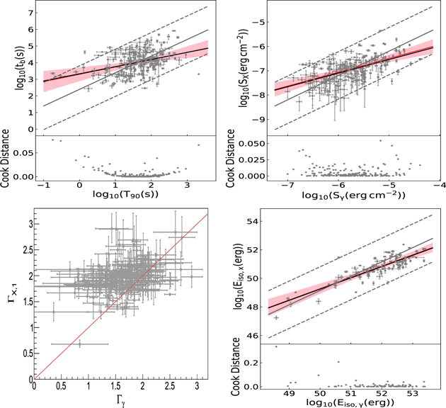
Figure 3. Parameter relationship between the shallow decay phase and the prompt emission phase, including tb– , SX–
, SX– ,
,  , and
, and  –
– . The black solid line represents the best fit with the least square regression method. The red solid line presents the best fit with the bivariate linear regression method and the pink shadowed region shows the intrinsic scatter to the population
  . The gray lines mark the best fitting results (solid) and its 2σ linear correlation region (dotted), which is defined with
  , where y and x are the two quantities in question and A and
  are the mean and its 1σ standard error for the y–x correlation. The orange solid lines show y = x.
Download figure:
Standard image High-resolution image3.3. Test Physical Origin of the Shallow Decay Segment
We first check whether there is any spectral evolution between shallow decay segment and its follow-up segment. The left panel of Figure 4 plots ΓX,2 as a function of ΓX,1. We find that all GRBs in our sample fall in the 2σ linear correlation regions. The middle of Figure 4 shows the comparison between the distributions of ΓX,1 and ΓX,2. For L07's sample, the Kolmogorov–Smirnov test suggests that these two distributions are consistent with the significance level of 0.96. With the larger sample, we find that the two distributions are still consistent, but the significance level of this consistency decreases to 0.40. As suggested by L07, here we define a new parameter as

to verify this consistency within the observational uncertainty for individual bursts. The right panel of Figure 4 shows μ distribution. We find that 84% of GRBs in our sample have  , and only 2 GRBs (GRB 080903 and GRB 150201A) show significant spectral evolution (
 ). Considering all of this evidence, we confirm L07's conclusion that there is no significant spectral evolution between the shallow decay segment and its follow-up segment, indicating that the shallow decay phase is a refreshed forward shock (Dai & Lu 1998; Rees & Mészáros 1998; Zhang & Mészáros 2001; Nousek et al. 2006; Zhang et al. 2006).
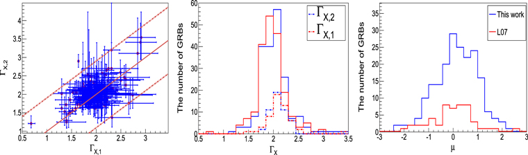
Figure 4. Left panel: comparison between ΓX,1 and ΓX,2. The orange lines represent  (solid) and its 2σ region (dotted). Middle panel: the distribution of ΓX,1 and ΓX,2, with solid lines showing our results and dotted lines showing L07's results. Right panel: the distribution of μ.
Download figure:
Standard image High-resolution imageIn this scenario, the shallow decay's follow-up segment should be consistent with the predictions of the forward shock models, namely the observed spectral index  and temporal decay index
  should follow the so-called "closure relations" (Gao et al. 2013, for a review). Although the closure correlations vary for different spectral regimes, different cooling schemes or different properties of the ambient medium, as illustrated in L07, three regimes are relevant here:
- 1.regime 1:
 (for either ISM or wind medium), where
- 2.regime 2: (for ISM medium), where
- 3.regime 3: (for wind medium), where .

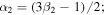


We define a new parameter  to test how well individual bursts being consistent with the closure relations under regime
  :
:

where  and
and  are the temporal decay slope from the observations and from the closure relations, and
  and
and  represent their uncertainties. For an individual burst, if there exists
  , we conclude that this burst belongs to the regime i model within 3σ significance. For those bursts that have more than one regime satisfying
  , we choose the regime with the smallest ϕ value.
Overall, we find that 66/198 bursts belong to regime 1, 82/198 bursts belong to regime 2, and 45/198 bursts belong to regime 3. For the other 5 bursts, we test their consistency with the curvature effect curve  (Kumar & Panaitescu 2000; Panaitescu et al. 2006) with the ϕ parameter. We find that three bursts cannot be excluded within 3σ significance by the curvature effect regime. These bursts could still be interpreted with the external-shock model once the jet break effect is invoked. We name regime 4 for these bursts. The other two bursts that could be excluded within 3σ significance by the curvature effect regime are difficult to interpret under an external-shock framework. As suggested by many previous works, the early X-ray plateau for these cases should be of internal origin and is directly connected to a long-lasting central engine (Troja et al. 2007; Rowlinson et al. 2010, 2013, 2014; Dall'Osso et al. 2011; Gompertz et al. 2013, 2014, 2015; Lü & Zhang 2014; Lü et al. 2015; Rea et al. 2015; Gibson et al. 2017, 2018; Gompertz & Fruchter 2017; Li et al. 2018; Stratta et al. 2018). We did not assign these bursts into either regime. Above all, we divided the GRBs of our sample into four groups, case1, case2, case3, and
  . Which case of each GRB in our sample belongs to and which regime is consistent with are list in Table 2. The relationships of αX,2 and
  in difference cases are shown in Figure 5.
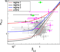
Figure 5. Temporal decay index αX,2 as a function of the spectral index  for shallow decay's follow-up segment, compared with the closure correlations of various spectral regimes. The gray dots show GRBs belonging to regimes 1–3 (case1). Pink dots show GRBs whose shallow decay segment and follow-up segment belongs to different spectrum regimes (case2). Black dots show GRBs that do not belong to regime 1–3 but that cannot be excluded within 3σ significance by the curvature effect regime (case3). Green dots show GRBs that could be excluded within 3σ significance by the curvature effect regime (case4).
Download figure:
Standard image High-resolution imageThe normal decay phases for 196/198 bursts in our sample are consistent with the external-shock models, inferring that their shallow decay phase might also be of external origin and may be related to continuous energy injection from the central engine. Here we assume that the central engine has a power-law luminosity release history as  , so that the injected energy would be
  (Zhang & Mészáros 2001). When
  is larger than the impulsively injected energy during the prompt emission phase, the dynamics of the external shock wave would be related to q as
  (
( ) and
) and  (
( ) for the ISM (wind) case. Consequently, we have
  (
( ),
),  (
( ), and
  (
( ) for the ISM (wind) models for p > 2, and
 ,
,  (
( ), and
  (
( ) for the ISM (wind) models for
  , where p is the electronic power-law index, and
  is the observed peak flux. The relationship between decay slope α and energy injection index q for different spectral regimes could thus be derived (see the results in Tables 13–16 of Gao et al. 2013).
In this case, the decay indices difference between the shallow decay segment and its follow-up segment in different regimes would be (Gao et al. 2013).
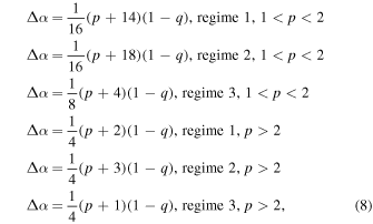
where p could be derived from the observed spectral index, depending on the observed spectral regime. Given the regime models for each burst (here we only test bursts in regimes 1–3), its energy injection parameter q could be thus derived based on αX,1 and αX,2. The upper panels of Figure 6 show the distributions of these GRBs in the two-dimensional q–Δα and q–p planes along with the contours of constant p and Δα. The distribution of derived p and q values are plotted in the lower panels of Figure 6. We find that q values are mainly distributed between −0.5 and 0.5, with an average value of 0.16 ± 0.12, which is consistent with the model prediction (q value around zero) where a spinning-down pulsar acts as the energy injection central engine (Dai & Lu 1998; Zhang & Mészáros 2001). With the derived q value, we can further test whether the αX,1 and  satisfy the corresponding closure relations with energy injection (see Table 14 and 16 in Gao et al. 2013) with the ϕ parameter. It turns out the shallow decay phases for all 194 GRBs satisfy the closure relations with energy injection, and their corresponding spectral regime for 189/196 (96.4%) bursts are consistent with their follow-up phases, which is expected because there is no systematic spectral evolution between these two segments.9
The results reinforce the conclusion that the shallow decay segment in most bursts is consistent with an external forward shock origin, probably due to a continuous energy injection from a long-lived central engine.
satisfy the corresponding closure relations with energy injection (see Table 14 and 16 in Gao et al. 2013) with the ϕ parameter. It turns out the shallow decay phases for all 194 GRBs satisfy the closure relations with energy injection, and their corresponding spectral regime for 189/196 (96.4%) bursts are consistent with their follow-up phases, which is expected because there is no systematic spectral evolution between these two segments.9
The results reinforce the conclusion that the shallow decay segment in most bursts is consistent with an external forward shock origin, probably due to a continuous energy injection from a long-lived central engine.

Figure 6. Upper panels: distributions of bursts in regimes 1–3 in the two-dimensional q–Δα and q–p planes, along with the model prediction for  (thick solid lines) and
  (thin solid lines). Lower panels: distributions of p values and q values.
Download figure:
Standard image High-resolution image3.4. Empirical Relations Revisited
3.4.1. Empirical Relation among , and


Based on their sample, L07 have investigated the relations among the energies  and
and  and other parameters
  and
and  , with a regression model as

where  ,
,  , and
, and  are multiple regression coefficients. The probability from a t-test (pt) was invoked to measure the significance of the dependence of each variable on the model and the probability from an F-test (pF) was invoked to justify the global regression of the three-parameter relation. For the
  relation, L07 yields
  (
( ) and
) and  ,
,  , and the pF is less than 10−4. Their results suggest a strong correlation between
  and
and  but a tentative correlation between
  and
and  , and thus a tentative global three-parameter correlation. We apply the regression model to our sample, we yield
  (
( ),
),  , and
, and  , with
  ,
,  , and
, and  . We find that with a larger sample, a strong correlation between
  and
and  still exists but the tentative correlation between
  and
and  has completely disappeared, so that the global three-parameter correlation becomes less significant. Note that in Dainotti et al. (2011b) it was already clear that
  was a weak correlation, while
  was a stronger correlation. Dainotti et al. (2016) thus proposed the
  correlation given the already established two-parameter
  (e.g., Dainotti et al. 2008) and
  correlations (Dainotti et al. 2011b, 2015). With an extended sample (updated to 2016 July) of long GRBs with X-ray plateau, Dainotti et al. (2017) yielded
  , with the Pearson correlation coefficient r = 0.90 with a probability of the same sample occurring by chance,
  .
.
For the  relation, L07 yields
  (
( ) and
) and  ,
,  , and the pF is less than 10−4. Their results suggest a strong correlation between
  and
and  but no correlation between
  and
and  . A tentative global three-parameter correlation might exist. With a larger sample, we yield
  (
( ),
),  , and
, and  , with
  ,
,  , and
, and  . We confirm that a strong correlation between
  and
and  and a tentative global three-parameter correlation exist and there is no correlation between
  and
and  . The data and regression modeling results are shown in Figure 7. It is worth noticing that Dainotti et al. (2011b) also investigated the
  –
– relation with 62 long GRBs with known redshift, and the correlation coefficient and the random occurrence probability p for their sample are
  and p = 0.1, also inferring that the correlation between
  and
and  was very weak.
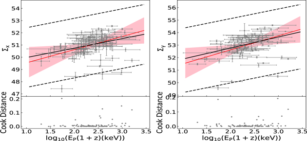
Figure 7. Left panel: the correlation between  and
and  . Right panel: the correlation between
  and
and  . The black lines represent the best fitting results (solid) and its 3σ uncertainty region (dotted) with least square regression method. The red line presents the best fitting results with the bivariate linear regression method and the pink shadowed region shows the intrinsic scatter to the population
  .
.
Download figure:
Standard image High-resolution image3.4.2. Revisit Correlations between (tb), LX, and


Dainotti et al. (2008) discovered a formal anticorrelation between X-ray luminosity at the end of plateau LX and rest frame plateau end time  , described as
  . Dainotti et al. (2010) fitted the correlation between LX and
  and achieved the results
  ,
,  . It is of interest to justify this empirical relationship with our updated sample. With the multivariate linear regression method, we find that the anticorrelation indeed exists between LX and
  , with
  (
( ) and
) and  , where
  ,
,  , and
, and  . In addition, the LX for individual GRBs in our sample are listed in Table 3. Basically speaking, our results in general agree well with Dainotti et al. (2013a), indicating that an intrinsic relationship between LX and
  indeed exist. This correlation has been tested against selection bias robustly (Dainotti et al. 2013a). It is worth noticing that LX is roughly inversely proportional to the timescale of the energy injection, inferring that the energy reservoir should be roughly a constant. This is consistent with the energy injection model, where the central engine is a newborn magnetar (Dai 2004).
Table 3. Part I: Rest-frame Properties for Bursts with Known Redshifts
| GRB Name |

|

|

|

|

|

|

|
|---|---|---|---|---|---|---|---|
| (s) | (keV) | (erg) | (erg) | (erg) | (s) | (erg s−1) | |
| 050319 | 0.37 ± 0.08 | 2.15 ± 0.18 | 52.23 ± 0.04 | 52.58 ± 0.08 | 51.82 ± 0.06 | 3.89 ± 0.06 | 47.05 ± 0.05 |
| 050401 | 0.93 ± 0.03 | 2.72 ± 0.1 | 53.39 ± 0.04 | 53.77 ± 0.04 | 52.06 ± 0.05 | 3.08 ± 0.04 | 48.13 ± 0.03 |
| 050416A | 0.16 ± 0.03 | 1.31 ± 0.17 | 50.47 ± 0.03 | 50.91 ± 0.06 | 49.52 ± 0.17 | 3 ± 0.14 | 46.21 ± 0.11 |
| 050505 | 1.06 ± 0.01 | 2.85 ± 0.13 | 53.13 ± 0.04 | 53.55 ± 0.05 | 51.88 ± 0.1 | 3.59 ± 0.07 | 47.43 ± 0.08 |
| 050714B | 1.13 | 1.8 ± 0.22 | 51.93 ± 0.09 | 52.3 ± 0.09 | 50.13 ± 0.18 | 4.03 ± 0.19 | 45.53 ± 0.13 |
| 050802 | 0.68 ± 0.06 | 2.46 ± 0.13 | 52.29 ± 0.04 | 52.65 ± 0.06 | 51.18 ± 0.18 | 3.29 ± 0.04 | 47.38 ± 0.06 |
| 050814 | 1.01 ± 0.12 | 2.64 ± 0.17 | 52.99 ± 0.07 | 53.33 ± 0.11 | 51.54 ± 0.08 | 4.15 ± 0.06 | 46.35 ± 0.08 |
| 050822 | 1.62 ± 0.01 | 1.71 ± 0.14 | 52.24 ± 0.04 | 52.59 ± 0.04 | 50.7 ± 0.09 | 3.89 ± 0.08 | 46.34 ± 0.07 |
| 050824 | 1.14 ± 0.08 | 1.46 ± 0.27 | 50.6 ± 0.09 | 51 ± 0.11 | 50.07 ± 0.17 | 4.56 ± 0.16 | 45.2 ± 0.1 |
| 050826 | 1.43 ± 0.09 | 2.59 ± 0.38 | 49.95 ± 0.07 | 50.55 ± 0.5 | 48.39 ± 0.18 | 4.51 ± 0.15 | 43.83 ± 0.15 |
| 051109B | 1.14 ± 0.03 | 1.74 ± 0.23 | 48.58 ± 0.06 | 48.92 ± 0.09 | 47.25 ± 0.12 | 3.46 ± 0.1 | 43.72 ± 0.09 |
| 051221A | −0.04 | 2.79 ± 0.14 | 51.38 ± 0.01 | 52.09 ± 0.07 | 49.69 ± 0.09 | 4.45 ± 0.08 | 44.78 ± 0.08 |
| 060108 | 0.68 ± 0.03 | 2.15 ± 0.17 | 51.55 ± 0.05 | 51.89 ± 0.05 | 50.53 ± 0.1 | 3.63 ± 0.1 | 46.34 ± 0.08 |
| 060115 | 1.5 ± 0.02 | 2.53 ± 0.14 | 52.67 ± 0.02 | 53 ± 0.11 | 51.07 ± 0.19 | 3.84 ± 0.18 | 46.27 ± 0.16 |
| 060306 | 1.38 ± 0.01 | 2.2 ± 0.13 | 52.11 ± 0.02 | 52.46 ± 0.08 | 50.54 ± 0.17 | 3.11 ± 0.16 | 46.97 ± 0.14 |
| 060502A | 1.12 ± 0.06 | 2.6 ± 0.12 | 52.09 ± 0.02 | 52.53 ± 0.05 | 51.08 ± 0.11 | 4.17 ± 0.11 | 46.2 ± 0.1 |
| 060604 | 0.5 ± 0.11 | 2.25 ± 0.34 | 51.13 ± 0.09 | 51.46 ± 0.18 | 50.72 ± 0.11 | 3.83 ± 0.08 | 46.37 ± 0.08 |
| 060605 | 0.5 ± 0.05 | 2.98 ± 0.19 | 52.1 ± 0.04 | 52.57 ± 0.1 | 51.52 ± 0.03 | 3.25 ± 0.03 | 47.41 ± 0.03 |
| 060607A | 1.39 ± 0.02 | 2.79 ± 0.11 | 52.71 ± 0.02 | 53.16 ± 0.05 | 52.37 ± 0.03 | 3.5 ± 0.01 | 48.08 ± 0.02 |
| 060614 | 1.95 | 2.53 ± 0.26 | 51.16 ± 0.02 | 51.71 ± 0.13 | 49.03 ± 0.03 | 4.64 ± 0.02 | 44.34 ± 0.03 |
| 060707 | 1.19 ± 0.03 | 2.47 ± 0.62 | 52.6 ± 0.05 | 52.95 ± 0.09 | 51.64 ± 0.16 | 4.45 ± 0.16 | 46.18 ± 0.15 |
| 060714 | 1.49 ± 0.02 | 2.25 ± 0.13 | 52.68 ± 0.03 | 52.99 ± 0.01 | 51.13 ± 0.11 | 3.1 ± 0.1 | 47.35 ± 0.11 |
| 060719 | 1.34 ± 0.04 | 2.08 ± 0.13 | 51.97 ± 0.03 | 52.28 ± 0.01 | 50.49 ± 0.12 | 3.47 ± 0.1 | 46.47 ± 0.1 |
| 060729 | 1.88 ± 0.04 | 1.98 ± 0.15 | 51.3 ± 0.03 | 51.63 ± 0.07 | 50.9 ± 0.02 | 4.61 ± 0.01 | 46.04 ± 0.01 |
| 060805A | 0.2 ± 0.04 | 2.04 ± 0.31 | 50.98 ± 0.11 | 51.33 ± 0.22 | 50.06 ± 0.16 | 3.03 ± 0.14 | 46.45 ± 0.15 |
| 060814 | 1.66 ± 0.01 | 2.88 ± 0.49 | 53.37 ± 0.02 | 53.89 ± 0.1 | 51.23 ± 0.07 | 3.64 ± 0.05 | 47.02 ± 0.06 |
| 060906 | 0.97 ± 0.01 | 2.33 ± 0.14 | 52.76 ± 0.03 | 53.09 ± 0.01 | 51.01 ± 0.05 | 3.38 ± 0.05 | 46.89 ± 0.05 |
| 060908 | 0.83 ± 0.01 | 2.77 ± 0.11 | 52.39 ± 0.01 | 52.84 ± 0.05 | 50.85 ± 0.11 | 2.38 ± 0.08 | 47.85 ± 0.09 |
| 060927 | 0.54 ± 0.01 | 2.67 ± 0.62 | 52.72 ± 0.04 | 53.06 ± 0.03 | 51.32 ± 0.14 | 2.98 ± 0.12 | 47.1 ± 0.15 |
| 061121 | 1.54 ± 0.03 | 3.15 ± 0.14 | 52.77 ± 0.01 | 53.58 ± 0.04 | 51.48 ± 0.05 | 3.34 ± 0.04 | 47.65 ± 0.05 |
| 061201 | −0.14 ± 0.05 | 2.99 ± 0.2 | 48.96 ± 0.04 | 49.86 ± 0.12 | 48.58 ± 0.08 | 3.4 ± 0.06 | 44.9 ± 0.09 |
| 061222A | 1.37 ± 0.02 | 3 ± 0.21 | 52.92 ± 0.01 | 53.57 ± 0.05 | 52.1 ± 0.03 | 4.19 ± 0.03 | 46.96 ± 0.03 |
| 070103 | 0.72 ± 0.02 | 2.23 ± 0.19 | 51.70 ± 0.06 | 52.03 ± 0.06 | 50.49 ± 0.08 | 2.6 ± 0.06 | 47.44 ± 0.05 |
| 070110 | 1.4 ± 0.02 | 2.58 ± 0.15 | 52.3 ± 0.03 | 52.66 ± 0.07 | 51.48 ± 0.02 | 3.79 ± 0.01 | 47.22 ± 0.02 |
| 070129 | 2.14 ± 0.02 | 2.16 ± 0.16 | 52.58 ± 0.04 | 52.90 ± 0.15 | 50.88 ± 0.08 | 3.73 ± 0.06 | 46.61 ± 0.05 |
| 070306 | 0.48 ± 0.09 | 2.33 ± 0.13 | 50.92 ± 0.25 | 51.26 ± 0.09 | 51.46 ± 0.03 | 4.08 ± 0.02 | 46.94 ± 0.02 |
| 070508 | 1.06 ± 0.02 | 2.67 ± 0.33 | 52.52 ± 0.01 | 53.07 ± 0.11 | 50.79 ± 0.33 | 2.2 ± 0.24 | 48.35 ± 0.16 |
| 070529 | 1.49 ± 0.01 | 2.8 ± 0.2 | 52.55 ± 0.04 | 53 ± 0.11 | 50.75 ± 0.15 | 2.48 ± 0.11 | 47.69 ± 0.12 |
| 070809 | 0.03 ± 0.03 | 2.02 ± 0.22 | 49.05 ± 0.04 | 49.39 ± 0.25 | 48.24 ± 0.15 | 3.69 ± 0.13 | 44.53 ± 0.11 |
| 070810A | 0.54 ± 0.04 | 2.14 ± 0.15 | 51.87 ± 0.04 | 52.21 ± 0.04 | 50.61 ± 0.21 | 2.64 ± 0.17 | 47.38 ± 0.19 |
| 080413B | 0.58 ± 0.05 | 2.19 ± 0.18 | 52 ± 0.01 | 52.34 ± 0.02 | 50.34 ± 0.14 | 2.28 ± 0.1 | 47.83 ± 0.08 |
| 080430 | 0.96 ± 0.06 | 2.15 ± 0.12 | 51.25 ± 0.04 | 51.6 ± 0.07 | 50.42 ± 0.07 | 4.28 ± 0.06 | 45.68 ± 0.05 |
| 080516 | 0.14 ± 0.02 | 2.44 ± 0.25 | 51.73 ± 0.06 | 52.07 ± 0.14 | 50.79 ± 0.17 | 3.12 ± 0.16 | 47 ± 0.14 |
| 080707 | 1.08 ± 0.02 | 2.21 ± 0.2 | 51.3 ± 0.05 | 52.61 ± 0.12 | 50.1 ± 0.16 | 3.68 ± 0.14 | 45.97 ± 0.12 |
| 080905B | 1.58 ± 0.05 | 2.38 ± 0.16 | 52.35 ± 0.05 | 52.7 ± 0.12 | 51.88 ± 0.07 | 3.64 ± 0.07 | 47.5 ± 0.05 |
| 081007 | 0.82 ± 0.16 | 1.5 ± 0.17 | 50.7 ± 0.05 | 51.06 ± 0.07 | 50.1 ± 0.3 | 4.44 ± 0.12 | 45.09 ± 0.12 |
| 081029 | 1.75 ± 0.07 | 2.88 ± 0.21 | 52.77 ± 0.04 | 53.22 ± 0.15 | 51.46 ± 0.03 | 3.53 ± 0.02 | 47.2 ± 0.03 |
| 090102 | 1.03 ± 0.03 | 2.68 ± 0.12 | 50.6 ± 0.02 | 51.06 ± 0.05 | 51.46 ± 0.06 | 2.75 ± 0.03 | 48.16 ± 0.04 |
| Part II: Rest-frame Properties for Bursts with Known Redshifts | |||||||
| 090113 | 0.52 ± 0.04 | 2.46 ± 0.13 | 51.75 ± 0.02 | 52.12 ± 0.05 | 50.51 ± 0.1 | 2.31 ± 0.08 | 47.81 ± 0.07 |
| 090205 | 0.19 ± 0.08 | 2.31 ± 0.2 | 51.85 ± 0.06 | 52.18 ± 0.1 | 51.19 ± 0.11 | 3.43 ± 0.1 | 46.77 ± 0.11 |
| 090313 | 1.25 ± 0.09 | 2.39 ± 0.26 | 52.5 ± 0.06 | 52.80 ± 0.1 | 51.46 ± 0.1 | 4.25 ± 0.06 | 46.64 ± 0.09 |
| 090404 | 1.32 ± 0.07 | 2.04 ± 0.13 | 52.75 ± 0.01 | 53.08 ± 0.05 | 51.36 ± 0.1 | 3.63 ± 0.08 | 47.06 ± 0.07 |
| 090407 | 2.1 ± 0.09 | 2.29 ± 0.27 | 51.75 ± 0.07 | 52.12 ± 0.27 | 50.93 ± 0.05 | 4.47 ± 0.05 | 45.89 ± 0.04 |
| 090418A | 1.33 ± 0.04 | 2.56 ± 0.11 | 52.46 ± 0.02 | 52.87 ± 0.04 | 51.31 ± 0.08 | 3.07 ± 0.06 | 47.64 ± 0.08 |
| 090424 | 1.53 | 2.44 ± 0.01 | 52.35 ± 0.25 | 52.8 ± 0.01 | 50.78 ± 0.18 | 2.79 ± 0.17 | 47.73 ± 0.16 |
| 090429B | −0.28 ± 0.07 | 2.64 ± 0.56 | 52.51 ± 0.04 | 52.83 ± 0.01 | 50.98 ± 0.1 | 1.88 ± 0.08 | 48.34 ± 0.04 |
| 090510 | −0.8 ± 0.12 | 3.07 ± 0.3 | 50.84 ± 0.05 | 51.46 ± 0.13 | 50.47 ± 0.07 | 2.91 ± 0.05 | 47.03 ± 0.06 |
| 090529 | 1.44 | 2.23 ± 0.25 | 52 ± 0.1 | 52.34 ± 0.11 | 50.81 ± 0.19 | 2.91 ± 0.05 | 47.03 ± 0.18 |
| 090530 | 1.33 ± 0.24 | 2.37 ± 0.19 | 51.64 ± 0.04 | 52 ± 0.26 | 50.7 ± 0.11 | 4.42 ± 0.1 | 45.47 ± 0.09 |
| 091018 | 0.35 ± 0.06 | 1.58 ± 0.57 | 51.52 ± 0.03 | 51.91 ± 0.38 | 50.56 ± 0.08 | 2.49 ± 0.07 | 47.65 ± 0.06 |
| 091029 | 1.02 ± 0.05 | 2.36 ± 0.41 | 52.59 ± 0.02 | 52.93 ± 0.05 | 51.17 ± 0.06 | 3.5 ± 0.05 | 47.06 ± 0.04 |
| 100219A | 0.52 ± 0.1 | 3.05 ± 0.29 | 52.14 ± 0.07 | 52.61 ± 0.31 | 51.83 ± 0.07 | 3.77 ± 0.03 | 47.05 ± 0.06 |
| 100302A | 0.49 ± 0.04 | 2.67 ± 0.2 | 52.09 ± 0.05 | 52.4 ± 0.15 | 50.94 ± 0.22 | 3.58 ± 0.22 | 46.47 ± 0.16 |
| 100418A | 0.63 ± 0.06 | 1.76 ± 0.21 | 50.52 ± 0.6 | 50.83 ± 0.13 | 49.79 ± 0.22 | 4.7 ± 0.06 | 44.95 ± 0.05 |
| 100425A | 1.13 ± 0.03 | 1.81 ± 0.24 | 51.54 ± 0.08 | 51.91 ± 0.21 | 50.41 ± 0.18 | 4.07 ± 0.18 | 45.63 ± 0.14 |
| 100901A | 2.26 ± 0.03 | 2.41 ± 0.22 | 52 ± 0.06 | 52.35 ± 0.32 | 51.24 ± 0.02 | 4.2 ± 0.02 | 46.72 ± 0.01 |
| 100906A | 1.62 ± 0.01 | 2.29 ± 0.1 | 53.12 ± 0.25 | 53.46 ± 0.04 | 51.46 ± 0.04 | 3.66 ± 0.03 | 47.02 ± 0.05 |
| 110106B | 1.19 ± 0.08 | 2.08 ± 0.14 | 51.28 ± 0.02 | 51.62 ± 0.1 | 50.14 ± 0.11 | 3.91 ± 0.1 | 45.76 ± 0.1 |
| 110808A | 1.31 ± 0.17 | 1.81 ± 0.3 | 51.17 ± 0.09 | 51.52 ± 0.24 | 50.43 ± 0.21 | 4.85 ± 0.21 | 44.86 ± 0.16 |
| 111008A | 1.03 ± 0.01 | 2.56 ± 0.12 | 53.35 ± 0.02 | 53.68 ± 0.01 | 52.05 ± 0.06 | 3.12 ± 0.06 | 48.04 ± 0.05 |
| 111228A | 1.77 ± 0.02 | 1.71 ± 0.12 | 52.04 ± 0.01 | 52.4 ± 0.07 | 50.66 ± 0.05 | 3.89 ± 0.05 | 46.37 ± 0.04 |
| 120326A | 1.4 ± 0.05 | 2.06 ± 0.19 | 52.3 ± 0.05 | 52.64 ± 0.01 | 51.57 ± 0.05 | 4.27 ± 0.01 | 46.96 ± 0.01 |
| 120521C | 0.58 ± 0.07 | 2.75 ± 0.13 | 52.78 ± 0.04 | 53.12 ± 0.12 | 51 ± 0.24 | 3.22 ± 0.23 | 46.81 ± 0.17 |
| 120811C | 0.86 ± 0.06 | 2.2 ± 0.2 | 52.67 ± 0.04 | 52.96 ± 0.01 | 51.17 ± 0.2 | 2.77 ± 0.17 | 47.74 ± 0.13 |
| 120907A | 0.93 ± 0.18 | 2.2 ± 0.2 | 51.2 ± 0.07 | 51.53 ± 0.2 | 50.27 ± 0.2 | 4.35 ± 0.17 | 45.45 ± 0.1 |
| 121024A | 1.54 ± 0.17 | 2.52 ± 0.25 | 51.42 ± 0.04 | 51.87 ± 0.25 | 50.63 ± 0.2 | 4.35 ± 0.17 | 45.45 ± 0.18 |
| 121128A | 0.86 ± 0.03 | 2.31 ± 0.14 | 52.88 ± 0.03 | 53.22 ± 0.01 | 51.43 ± 0.07 | 2.7 ± 0.05 | 48.06 ± 0.06 |
| 121211A | 1.95 ± 0.08 | 1.72 ± 0.21 | 51.53 ± 0.08 | 51.88 ± 0.19 | 50.56 ± 0.14 | 4.32 ± 0.11 | 45.69 ± 0.11 |
| 130603B | −0.88 ± 0.05 | 3.2 ± 0.15 | 50.29 ± 0.02 | 51.29 ± 0.11 | 49.58 ± 0.06 | 3.23 ± 0.05 | 46.08 ± 0.06 |
| 131105A | 1.62 ± 0.02 | 2.61 ± 0.14 | 52.69 ± 0.03 | 53.14 ± 0.07 | 50.77 ± 0.1 | 3.23 ± 0.08 | 47.1 ± 0.08 |
| 140430A | 1.82 ± 0.01 | 2.09 ± 0.2 | 51.83 ± 0.08 | 52.16 ± 0.07 | 50.86 ± 0.17 | 4.26 ± 0.16 | 45.86 ± 0.16 |
| 140512A | 1.95 ± 0.01 | 2.41 ± 0.09 | 52.27 ± 0.01 | 52.71 ± 0.04 | 51.4 ± 0.06 | 3.88 ± 0.06 | 46.92 ± 0.06 |
| 140518A | 1.03 ± 0.02 | 2.4 ± 0.4 | 52.58 ± 0.04 | 52.92 ± 0.01 | 50.94 ± 0.16 | 2.53 ± 0.12 | 47.86 ± 0.08 |
| 140703A | 1.21 ± 0.3 | 2.51 ± 0.15 | 52.9 ± 0.03 | 53.21 ± 0.1 | 52.13 ± 0.04 | 3.54 ± 0.03 | 47.66 ± 0.04 |
| 141121A | 2.35 ± 0.03 | 2.3 ± 0.15 | 52.45 ± 0.03 | 52.78 ± 0.12 | 51.18 ± 0.07 | 5.13 ± 0.05 | 45.52 ± 0.07 |
| 150323A | 1.97 ± 0.03 | 2 ± 0.11 | 51.73 ± 0.01 | 52.06 ± 0.01 | 49.66 ± 0.13 | 3.96 ± 0.11 | 45.32 ± 0.09 |
| 150424A | 1.85 ± 0.09 | 2.55 ± 0.2 | 50.51 ± 0.03 | 51.09 ± 0.12 | 49.51 ± 0.2 | 4.94 ± 0.18 | 43.96 ± 0.17 |
| 150910A | 1.68 ± 0.13 | 2.58 ± 0.15 | 52.34 ± 0.04 | 52.81 ± 0.08 | 51.73 ± 0.15 | 3.56 ± 0.07 | 47.65 ± 0.12 |
| 151027A | 1.86 ± 0.02 | 2.17 ± 0.1 | 52.11 ± 0.04 | 52.46 ± 0.03 | 51.34 ± 0.02 | 3.34 ± 0.02 | 47.78 ± 0.02 |
| 151112A | 0.58 ± 0.42 | 2.57 ± 0.21 | 52.46 ± 0.05 | 52.81 ± 0.17 | 51.54 ± 0.18 | 4.06 ± 0.16 | 46.55 ± 0.15 |
| 160227A | 1.97 ± 0.09 | 2.35 ± 0.33 | 52.59 ± 0.03 | 52.90 ± 0.04 | 51.63 ± 0.1 | 3.85 ± 0.09 | 47.18 ± 0.08 |
| 160327A | 0.67 ± 0.12 | 2.58 ± 0.14 | 52.78 ± 0.03 | 53.09 ± 0.01 | 51.23 ± 0.13 | 2.84 ± 0.11 | 47.55 ± 0.13 |
| 160804A | 1.92 ± 0.05 | 1.96 ± 0.07 | 52.19 ± 0.01 | 52.49 ± 0.01 | 49.7 ± 0.1 | 3.72 ± 0.07 | 45.88 ± 0.04 |
| 161108A | 1.69 ± 0.05 | 2.13 ± 0.17 | 51.57 ± 0.04 | 51.91 ± 0.09 | 50.16 ± 0.15 | 4.03 ± 0.14 | 45.82 ± 0.08 |
| 161129A | 1.33 ± 0.02 | 2.27 ± 0.1 | 51.57 ± 0.01 | 51.96 ± 0.03 | 50.26 ± 0.09 | 3.34 ± 0.07 | 46.59 ± 0.11 |
| 170113A | 0.84 ± 0.08 | 2.34 ± 0.49 | 51.78 ± 0.04 | 52.13 ± 0.13 | 51.41 ± 0.07 | 3.16 ± 0.06 | 47.61 ± 0.06 |
| 170202A | 1 ± 0.1 | 2.61 ± 0.11 | 52.93 ± 0.01 | 53.28 ± 0.04 | 51.22 ± 0.07 | 2.65 ± 0.06 | 48.01 ± 0.04 |
Xu & Huang (2012) introduced a third parameter  to the above relation (replacing
  by tb) and claimed that the three-parameter correlation would be tighter. The relation could be expressed as
  , with
  ,
,  , and
, and  . We have also justified this empirical relationship with our updated sample. With multiple regression analysis methods, we find that the three-parameter correlation indeed exists, with
  ,
,  , and
, and  (
( ), where
  ,
,  , and
, and  . The data and fitting results regarding this relationship are shown in Figure 8. It is interesting to note that besides the Xu & Huang (2012) correlation, more recently Dainotti et al. (2016, 2017) showed that the
  correlation is 37% tighter than the Xu & Huang (2012) correlation, making the
  correlation the tighest correlation in the literature so far involving the plateau emission.
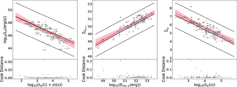
Figure 8. Left panel: the correlation between LX and  . Middle panel: the correlation between
  and
and  . Right panel: the correlation between
  and tb. The black lines represent the best fitting results (solid) and its 3σ uncertainty region (dotted) with the least square regression method. The red line presents the best fitting results with the bivariate linear regression method and the pink shadowed region shows the intrinsic scatter to the population
  .
.
Download figure:
Standard image High-resolution image4. Conclusions and Discussion
With Swift/XRT light curves of GRBs between 2004 February and 2017 July, we revisit the analysis of the shallow decay component from Liang et al. (2007). Our results and the comparison with L07's results are summarized as follows:
- 1.We find that with a larger sample, the distributions of the characteristic properties of the shallow decay phase (e.g., tb, SX, ΓX,1, and αX,1) still accord with normal or lognormal distribution with, , , and . Comparing with L07's results, the distributions for all the parameters become slightly broader but the peaks of each distribution barely change.
- 2.We find that with a larger sample, ΓX,1 and Γγ still show no correlation, with ΓX,1 systemically larger than Γγ. The tentative correlations of durations, energy fluences, and isotropic energies between the gamma-ray and X-ray phases still exist, but all correlations become significantly weaker than L07's results.
- 3.We find that for most GRBs, there is no significant spectral evolution between the shallow decay segment and its follow-up segment, and the follow-up segment for most bursts in our sample are consistent with the external-shock models. These two findings are consistent with L07's results, which infer that the shallow decay phase for most GRBs should be of external origin and may be related to continuous energy injection from the central engine.
- 4.Assuming that the central engine has a power-law luminosity release history as, we find that q values are mainly distributed between −0.5 and 0.5, with an average value of 0.16 ± 0.12, which is consistent with L07's results and is well consistent with the model prediction (q value around zero) where a spinning-down pulsar acts as the energy injection central engine (Dai & Lu 1998; Zhang & Mészáros 2001). With the derived q value, we find that the shallow decay phases for 196/198 GRBs satisfy the closure relations with energy injection, and their corresponding spectral regime for most bursts (96.4%) is consistent with their follow-up phases.
- 5.We find that with a larger sample, L07 suggested that a correlation between and still exists but the tentative correlation between and is completely disappeared, so that the global three-parameter correlation becomes less significant. On the other hand, we confirm that a strong correlation between and and a tentative global three-parameter correlation () exist but there is no correlation between and .
- 6.We find that the anticorrelation indeed exists between LX and (as suggested by Dainotti et al. 2008), with () and , where the pF is less than 10−4. Xu & Huang (2012) introduced a three-parameter correlation by inserting into the above relation (and replacing by tb) and we find that with our updated sample, the three-parameter correlation indeed exists, with , , and (), where the pF is . More recently Dainotti et al. (2016, 2017) showed that the correlation is 37% tighter than the Xu & Huang (2012) correlation, making the correlation the tightest correlation in the literature involving plateau emission. In addition, we note that this correlation is the result of two correlations that have been tested for selection bias.


In conclusion, with an updated sample, our results are consistent with most of L07's results and confirm their suggestion that the shallow decay segment in most bursts is consistent with an external forward shock origin, probably due to a continuous energy injection from a long-lived central engine.
This work was supported by the National Natural Science Foundation of China (under grant Nos. 11722324, 11603003, 11633001, 11690024, and 11603006), and the Strategic Priority Research Program of the Chinese Academy of Sciences (grant No. XDB23040100). L.H.J. acknowledges support by the GuangXi Science Foundation (grant Nos. 2017GXNSFFA198008 and 2016GXNSFCB380005), the One-Hundred-Talents Program of GuangXi colleges, and Bagui Young Scholars Program of GuangXi. B.B.Z. acknowledges support from National Thousand Young Talents program of China and National Key Research and Development Program of China (2018YFA0404204) and The National Natural Science Foundation of China (grant No. 11833003).
Software: XSPEC (Arnaud 1996), HEAsoft (v6.12; NASA High Energy Astrophysics Science Archive Research Center (HEASARC), 2014), root (v5.34; Brun & Rademakers 1997), Linmix_err (Kelly 2007).
Footnotes
- 5
- 6
We have tested that reasonably adjusting the criteria values of 0.8 and 0.4 might slightly change the size of the final sample but would not affect the main conclusions.
- 7
In our analysis, we have checked several different distribution functions, including Weibull distribution, Beta distribution, Gamma distribution, normal distribution, lognormal distribution, exponential distribution, and so on. We compare these distribution functions by comparing their fitting square error (the sum of squared discrepancies between histogram frequencies and fitted-distribution frequencies), and find that normal or lognormal functions are always the best or very close to the best to fit our interested distributions. In order to better compare our results with L07 findings, and considering that normal or lognormal functions have stronger physical meaning than other functions, here we only use normal and lognormal functions to fit relevant distributions.
- 8
2σ linear correlation regions are defined with
, where y and x are the two quantities in question and A and are the mean and its 1σ standard error for the y–x correlation. - 9
There are seven GRBs (050401, 060413, 071118, 100508A, 100902A, 110411A, and 161202A) whose shallow decay phase and normal decay phase belong to different spectral regimes. For GRBs 050401, 071118, 110411A, and 161202A, too few data points around tb might cause greater uncertainty for αX,2 and/or
. GRBs 060413, 100508A, and 100902A marginally belongs to regime 3 but with a large decay slope for the normal decay phase.


