


Abstract
We present the first results from a detailed analysis of a new, long (∼100 ks) XMM-Newton observation of the narrow-line Seyfert 1 galaxy PG 1404+226, which showed a large-amplitude, rapid X-ray variability by a factor of ∼7 in ∼10 ks with an exponential rise and a sharp fall in the count rate. We investigate the origin of the soft X-ray excess emission and rapid X-ray variability in the source through time-resolved spectroscopy and fractional rms spectral modeling. The strong soft X-ray excess below 1 keV observed in both the time-averaged and time-resolved spectra is described by the intrinsic disk Comptonization model as well as the relativistic reflection model where the emission is intense merely in the inner regions ( ) of an ionized accretion disk. We detected no significant UV variability, while the soft X-ray excess flux varies together with the primary power-law emission (as
  ), although with a smaller amplitude, as expected in the reflection scenario. The observed X-ray fractional rms spectrum is approximately constant with a drop at ∼0.6 keV and is described by a non-variable emission line component with the observed energy of ∼0.6 keV and two variable spectral components: a more variable primary power-law emission and a less variable soft excess emission. Our results suggest the "lamppost geometry" for the primary X-ray-emitting hot corona, which illuminates the innermost accretion disk due to strong gravity and gives rise to the soft X-ray excess emission.
Export citation and abstract BibTeX RIS
1. Introduction
The narrow-line Seyfert 1 (NLS1) galaxies, a subclass of active galactic nuclei (AGNs), have been of great interest because of their extreme variability in the X-ray band (Boller et al. 1996; Leighly 1999a; Komossa & Meerschweinchen 2000). The defining properties of this class of AGNs are: Balmer lines with FWHM(Hβ) < 2000 km s−1 (Osterbrock & Pogge 1985; Goodrich 1989), strong permitted optical/UV Fe ii emission lines (Boroson & Green 1992; Grupe et al. 1999; Véron-Cetty et al. 2001), and weaker [O iii] emission, ![$\tfrac{[{\rm{O}}\,{\rm{III}}]\lambda 5007}{{{\rm{H}}}_{\beta }}\leqslant 3$](https://content.cld.iop.org/journals/0004-637X/863/2/178/revision1/apjaad193ieqn3.gif) (Osterbrock & Pogge 1985; Goodrich 1989). The X-ray spectra of Seyfert galaxies show a power-law-like primary continuum, which is thought to arise due to thermal Comptonization of the optical/UV seed photons in a corona of hot electrons surrounding the central supermassive black hole (SMBH) (e.g., Haardt & Maraschi 1991, 1993). The optical/UV seed photons are thought to arise from an accretion disk (Shakura & Sunyaev 1973). However, the interplay between the accretion disk and the hot corona is not well understood. Many type 1 AGNs also show strong "soft X-ray excess" emission over the power-law continuum below ∼2 keV in their X-ray spectra. The existence of this component (∼0.1–2 keV) was discovered around 30 years ago (e.g., Arnaud et al. 1985; Singh et al. 1985), and its origin is still controversial. Initially, it was considered to be the high-energy tail of the accretion disk emission (Arnaud et al. 1985; Leighly 1999b), but the temperature of the soft X-ray excess is in the range ∼0.1–0.2 keV, which is much higher than the maximum disk temperature expected in AGNs. It was then speculated that the soft X-ray excess could result from the Compton up-scattering of the disk photons in an optically thick, warm plasma (e.g., Magdziarz et al. 1998; Janiuk et al. 2001). Currently, there are two competing models for the origin of the soft X-ray excess: optically thick, low-temperature Comptonization (Magdziarz et al. 1998; Dewangan et al. 2007; Done et al. 2012) and relativistic reflection from an ionized accretion disk (Fabian et al. 2002; Crummy et al. 2006; García et al. 2014; Mallick et al. 2018). However, these models sometimes give rise to spectral degeneracy because of the presence of multiple spectral components in the energy spectra of NLS1 galaxies (Dewangan et al. 2007; Ghosh et al. 2016). One efficient approach to overcome the spectral degeneracy is to study the rms spectrum, which links the energy spectrum with variability and has been successfully applied in a number of AGNs (MCG–6-30-15: Miniutti et al. 2007; 1H 0707–495: Fabian et al. 2012; RX J1633.3+4719: Mallick et al. 2016; Ark 120: Mallick et al. 2017). Observational evidence for the emission in different bands such as UV, soft and hard X-rays during large-variability events may help us to probe the connection between the disk, the hot corona, and the regions emitting the soft X-ray excess.
(Osterbrock & Pogge 1985; Goodrich 1989). The X-ray spectra of Seyfert galaxies show a power-law-like primary continuum, which is thought to arise due to thermal Comptonization of the optical/UV seed photons in a corona of hot electrons surrounding the central supermassive black hole (SMBH) (e.g., Haardt & Maraschi 1991, 1993). The optical/UV seed photons are thought to arise from an accretion disk (Shakura & Sunyaev 1973). However, the interplay between the accretion disk and the hot corona is not well understood. Many type 1 AGNs also show strong "soft X-ray excess" emission over the power-law continuum below ∼2 keV in their X-ray spectra. The existence of this component (∼0.1–2 keV) was discovered around 30 years ago (e.g., Arnaud et al. 1985; Singh et al. 1985), and its origin is still controversial. Initially, it was considered to be the high-energy tail of the accretion disk emission (Arnaud et al. 1985; Leighly 1999b), but the temperature of the soft X-ray excess is in the range ∼0.1–0.2 keV, which is much higher than the maximum disk temperature expected in AGNs. It was then speculated that the soft X-ray excess could result from the Compton up-scattering of the disk photons in an optically thick, warm plasma (e.g., Magdziarz et al. 1998; Janiuk et al. 2001). Currently, there are two competing models for the origin of the soft X-ray excess: optically thick, low-temperature Comptonization (Magdziarz et al. 1998; Dewangan et al. 2007; Done et al. 2012) and relativistic reflection from an ionized accretion disk (Fabian et al. 2002; Crummy et al. 2006; García et al. 2014; Mallick et al. 2018). However, these models sometimes give rise to spectral degeneracy because of the presence of multiple spectral components in the energy spectra of NLS1 galaxies (Dewangan et al. 2007; Ghosh et al. 2016). One efficient approach to overcome the spectral degeneracy is to study the rms spectrum, which links the energy spectrum with variability and has been successfully applied in a number of AGNs (MCG–6-30-15: Miniutti et al. 2007; 1H 0707–495: Fabian et al. 2012; RX J1633.3+4719: Mallick et al. 2016; Ark 120: Mallick et al. 2017). Observational evidence for the emission in different bands such as UV, soft and hard X-rays during large-variability events may help us to probe the connection between the disk, the hot corona, and the regions emitting the soft X-ray excess.
In this paper, we investigate the origin of the soft X-ray excess emission, the rapid X-ray variability, and the disk–corona connection in PG 1404+226 with the use of both model-dependent and model-independent techniques. PG 1404+226 is an NLS1 galaxy at a redshift z = 0.098 with FWHM(Hβ) ∼ 800 km s−1 (Wang et al. 1996). Previously, the source was observed with ROSAT (Ulrich-Demoulin & Molend 1996), ASCA (Leighly et al. 1997; Vaughan et al. 1999), Chandra (Dasgupta et al. 2005), and XMM-Newton (Crummy et al. 2005). From the ASCA observation, the 2–10 keV spectrum was found to be quite flat (Γ = 1.6 ± 0.4) with flux  erg cm−2 s−1 (Vaughan et al. 1999). The detection of an absorption edge at ∼1 keV was claimed in previous studies and interpreted as the high-velocity (0.2c–0.3c) outflow of ionized oxygen (Leighly et al. 1997). The source is well known for its strong soft X-ray excess and large-amplitude X-ray variability on short timescales (Ulrich-Demoulin & Molend 1996; Dasgupta et al. 2005). Here we explore the X-ray light curves, time-averaged as well as time-resolved energy spectra, fractional rms variability spectrum, and flux–flux plot through a new ∼100 ks XMM-Newton observation of PG 1404+226.
We describe the XMM-Newton observation and data reduction in Section 2. In Section 3, we present the analysis of the X-ray light curves and hardness ratio. In Section 4, we present time-averaged and time-resolved spectral analyses with the use of both phenomenological and physical models. In Sections 5 and 6, we present the flux−flux analysis and modeling of the X-ray fractional rms variability spectrum, respectively. Finally, we summarize and discuss our results in Section 7. Throughout the paper, the cosmological parameters H0 = 70 km s−1 Mpc−1, Ωm = 0.27, ΩΛ = 0.73 are adopted.
2. Observation and Data Reduction
We observed PG 1404+226 with the XMM-Newton telescope (Jansen et al. 2001) on 2016 January 25 (Obs. ID 0763480101) for an exposure time of ∼100 ks. Here we analyze data from the European Photon Imaging Camera (EPIC-PN: Strüder et al. 2001; EPIC-MOS: Turner et al. 2001), Reflection Grating Spectrometer (RGS: den Herder et al. 2001), and Optical Monitor (OM: Mason et al. 2001) on board XMM-Newton. We processed the raw data with the Scientific Analysis System (SAS v.15.0.0) and the most recent (as of 2016 August 2) calibration files. The EPIC-PN and MOS detectors were operated in the large- and small-window modes respectively using the thin filter. We processed EPIC-PN and MOS data using epproc and emproc respectively to produce the calibrated photon event files. We checked for photon pileup using the task epatplot and found no pileup in either the PN or MOS data. To filter the processed PN and MOS events, we included unflagged events with pattern ≤ 4 and pattern ≤ 12, respectively. We excluded the proton background flares by generating a GTI (good time interval) file above 10 keV for the full field with RATE <3.1 counts s−1, 1.3 counts s−1, and 2.1 counts s−1 for PN, MOS 1, and MOS 2, respectively, to obtain the maximum signal-to-noise ratio. It resulted in a filtered duration of ∼73 ks for both the cleaned EPIC-PN and MOS data. We extracted the PN and MOS source events from circular regions of radii 35 arcsec and 25 arcsec, respectively, centered on the source, while the background events were extracted from a nearby source-free circular region with a radius of 50 arcsec for both the PN and MOS data. We produced the redistribution matrix file (rmf) and ancillary region file (arf) with the tasks rmfgen and arfgen, respectively. We extracted the deadtime-corrected source and background light curves for different energy bands and bin times from the cleaned PN and MOS event files using the task epiclccorr. We combined the background-subtracted EPIC-PN, MOS 1, and MOS 2 light curves with the FTOOLS (Blackburn 1995) task lcmath. The source count rate was rather low above 8 keV, and therefore we considered only the 0.3−8 keV band for both the spectral and timing analyses. For spectral analysis, we used only the EPIC-PN data due to their higher signal-to-noise ratio compared to the MOS data. We grouped the average PN spectrum using the HEASOFT v.6.19 task grppha to have a minimum of 50 counts per energy bin. The net count rate estimated for EPIC-PN is 0.32 ± 0.03 counts s−1, resulting in a total of 1.65 × 10⁴ PN counts. Figure 1 shows the 0.3–8 keV EPIC-PN background-subtracted source (in red circles) and background (in black squares) spectra of PG 1404+226.
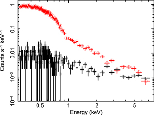
Figure 1. The 0.3–8 keV XMM-Newton/EPIC-PN background-subtracted source (in red circles) and background (in black squares) spectra of PG 1404+226 observed in 2016.
Download figure:
Standard image High-resolution imageWe processed the RGS data with the SAS task rgsproc. The response files were generated using the task rgsrmfgen. We combined the spectra and response files for two RGS 1+2 using the task rgscombine. Finally, we grouped the RGS spectral data using the grppha tool with a minimum of 50 counts per bin. This restricts the applicability of the χ2 statistics.
The OM was operated in the imaging fast mode using only the UVW1 (λeff ∼ 2910 Å) filter for a total duration of 94 ks. There are a total of 20 UVW1 exposures, and we found that only the last 14 exposures were acquired simultaneously with the filtered EPIC-PN data. We did not use the fast-mode OM data because of the presence of a variable background. We processed only the imaging-mode OM data with the SAS task omichain and obtained the background-subtracted count rate of the source, corrected for coincidence losses.
3. Timing Analysis: Light Curves and Hardness Ratio
We perform a timing analysis of PG 1404+226 to investigate the time and energy dependence of the variability. Figure 2 shows the 0.3–8 keV, background-subtracted, deadtime-corrected EPIC-PN, MOS 1, and MOS 2 light curves of PG 1404+226 with time bins of 500 s. The X-ray time series clearly shows a short-term, large-amplitude variability event in which PG 1404+226 varied by a factor of ∼7 in ∼10 ks during the 2016 observation. The fractional rms variability amplitude estimated in the 0.3–8 keV band is Fvar,X = (82.5 ± 1.4)%. The uncertainty on Fvar was calculated in accordance with Vaughan et al. (2003). Based on the variability pattern, we divided the entire ∼73 ks light curve into five intervals. Int 1 consists of the first 38 ks of the time series and has the lowest flux and moderate fractional rms variability of  . In Int 2, the X-ray flux increases exponentially by a factor of ∼3 with fractional rms variability of
  . The duration of Int 2 is ∼10 ks. During Int 3, the source was in the highest flux state with a fractional rms amplitude of
  . The source was in the brightest state for only ∼6 ks and then the count rate started decreasing. In Int 4, the source flux dropped by a factor of ∼3 in ∼6 ks with
  . At the end of the observation, the source was moderately variable with
  . In Figure 3, we show the UVW1 light curve of PG 1404+226 simultaneously with the X-ray light curve. The amplitude of the observed UV variability is only ∼3% of the mean count rate on a timescale of ∼62 ks. The fractional rms variability amplitude in the UVW1 band is
  , which is much less than the X-ray variability. The X-ray and UV variability patterns appear to be significantly different, suggesting the lack of any correlation between the X-ray and UV emission at zero time lag.
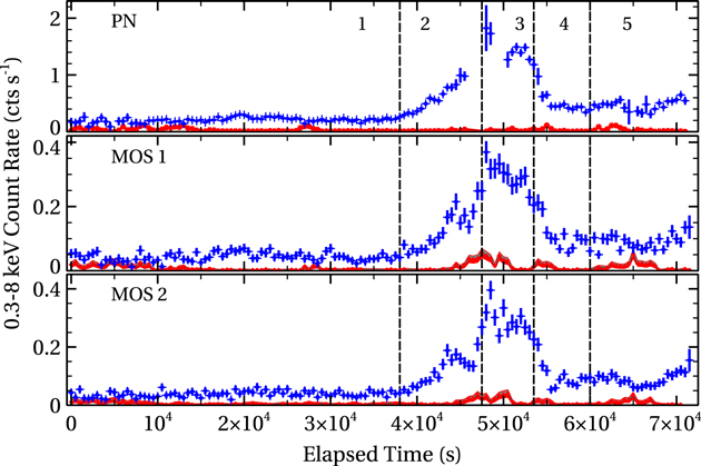
Figure 2. The 0.3–8 keV XMM-Newton/EPIC-PN, MOS 1, and MOS 2 background-subtracted, deadtime-corrected light curves of PG 1404+226 observed in 2016 with time bins of 500 s. The vertical lines indicate the margin between different characteristics of the time series. We show the corresponding background light curves in red.
Download figure:
Standard image High-resolution image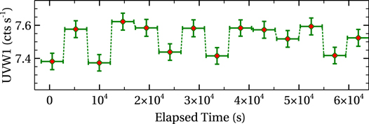
Figure 3. The background-subtracted UVW1 count rate of PG 1404+226 extracted from the imaging-mode OM exposures.
Download figure:
Standard image High-resolution imageThe upper and middle panels of Figure 4 show the background-subtracted, deadtime-corrected, combined EPIC-PN+MOS soft (0.3–1 keV) and hard (1–8 keV) X-ray light curves, respectively, with time bins of 2 ks. The soft band is observed to be brighter than the hard band; however, the variability pattern and amplitude ( and
and  ) in these two bands are found to be comparable during the observation. The peak-to-trough ratio of the variability amplitude in both the soft and hard bands is of the order of ∼12. In the bottom panel of Figure 4, we have shown the hardness ratio as a function of time. A constant model fitted to the curve of hardness ratio provided a statistically poor fit (χ2/dof = 46/29, dof = degrees of freedom), implying the presence of moderate spectral variability, and the source became harder at the beginning of the large-amplitude variability.
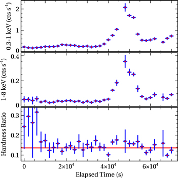
Figure 4. The upper and middle panels show the background-subtracted, deadtime-corrected, combined EPIC-PN+MOS light curves in the soft (0.3–1 keV) and hard (1–8 keV) bands, respectively. The bottom panel is the corresponding hardness ratio (1–8 keV/0.3–1 keV) as a function of the elapsed time, showing spectral variations. The time binning is 2 ks.
Download figure:
Standard image High-resolution image4. Spectral Analysis
We perform the spectral analysis of PG 1404+226 using XSPEC v.12.8.2 (Arnaud 1996). We employ the χ2 statistics and quote the errors at the 90% confidence limit for a single parameter corresponding to Δχ2 = 2.71 unless otherwise specified.
4.1. Phenomenological Model
4.1.1. The 0.3–8 keV EPIC-PN Spectrum
We begin our spectral analysis by fitting the 1–8 keV EPIC-PN spectrum using a continuum model (zpowerlw) multiplied by the Galactic absorption model (TBabs) using the cross sections and solar interstellar medium (ISM) abundances of Wilms et al. (2000). We fixed the Galactic column density at NH = 2.22 × 1020 cm−2 (Willingale et al. 2013) after accounting for the effect of molecular hydrogen. This model provided χ2 = 70 for 50 dof with Γ ∼ 1.81 and can be considered as a good baseline model to describe the hard X-ray emission from the source. Then we extrapolated our 1–8 keV absorbed power-law model (TBabs × zpowerlw) down to 0.3 keV. This extrapolation reveals the presence of a strong soft X-ray excess emission below 1 keV with χ2/dof = 11,741/160. We show the ratio of the observed EPIC-PN data and the absorbed power-law model in Figure 5 (top). The fitting of the full band (0.3–8 keV) data with the absorbed power-law model (TBabs × zpowerlw) resulted in a poor fit with χ2/dof = 1151.7/158. The residual plot demonstrates a sharp dip in the 0.8–1 keV band and an excess emission below 1 keV. Initially, we modeled the soft X-ray excess emission using a simple blackbody model (zbbody). The addition of the zbbody model improved the fit statistics to χ2/dof = 230.2/156 (Δχ2 = −921.5 for 2 dof). In XSPEC, the model reads as TBabs × (zbbody+zpowerlw). We show the deviations of the observed EPIC-PN data from the absorbed blackbody and power-law model in Figure 5 (middle). The estimated blackbody temperature  eV is consistent with the temperature of the soft X-ray excess emission observed in Seyfert 1 galaxies and QSOs (Czerny et al. 2003; Gierliński & Done 2004; Crummy et al. 2006; Papadakis et al. 2007). To model the absorption feature, we have created a warm absorber (WA) model for PG 1404+226 in XSTAR v.2.2.1 (last described by Kallman & Bautista 2001 and revised in 2015 July). The XSTAR photoionized absorption model has three free parameters: column density (NH), redshift (z), and ionization parameter (
 , where
  , L is the source luminosity, n is the hydrogen density, and r is the distance between the source and cloud). The inclusion of the WA significantly improved the fit statistics from χ2/dof = 230.2/156 to 173.7/154 (Δχ2 = −56.5 for 2 dof). To test the presence of any outflow, we varied the redshift of the absorbing cloud, which did not improve the fit statistics. We show the deviations of the observed EPIC-PN data from the model, TBabs × WA × (zbbody+zpowerlw) in Figure 5 (bottom). We notice significant positive residuals at ∼0.6 keV, which may be the signature of an emission feature. To model the emission feature, we added a Gaussian emission line (GL), which improved the fit statistics to χ2/dof = 154.6/152 (Δχ2 = −19.1 for 2 dof). The centroid energies of the emission line in the observed and rest frames are ∼0.6 keV and ∼0.66 keV, respectively. The rest-frame 0.66 keV emission feature most likely represents the O viii Lyα line. The EPIC-PN spectral data, the best-fit model, TBabs × WA × (GL+zbbody+zpowerlw), and the deviations of the observed data from the best-fit model are shown in Figure 6 (left). The best-fit values for the column density and ionization parameter of the WA are
  and
and  , respectively.

Figure 5. Top: the ratio of the EPIC-PN spectral data and absorbed power-law model [TBabs × zpowerlw] (Γ ∼ 1.81) fitted in the 1–8 keV band and extrapolated to lower energies. Middle: deviations of the observed PN data from the absorbed blackbody and power-law model [TBabs × (zbbody+zpowerlw)] fitted in the full band (0.3–8 keV). Bottom: deviations of the observed PN data from the full band (0.3–8 keV) model [TBabs × WA × (zbbody+zpowerlw)], showing an excess emission at around 0.6 keV in the observer's frame.
Download figure:
Standard image High-resolution image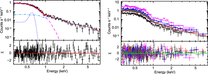
Figure 6. Left: the time-averaged EPIC-PN spectrum, the best-fit model, TBabs × WA × (GL+zbbody+zpowerlw), and the deviations of the observed data from the best-fit model (in red). The power-law, blackbody, and Gaussian emission components are shown as the dashed–dotted, dashed, and dotted lines, respectively. Right: the time-resolved EPIC-PN spectra, the best-fit model, TBabs × WA × (GL+zbbody+zpowerlw), and the residual spectra. The black squares, red circles, magenta triangles, blue crosses, and gray diamonds represent spectral data for Int 1, Int 2, Int 3, Int 4, and Int 5, respectively.
Download figure:
Standard image High-resolution imageTo search for spectral variability on shorter timescales, we performed time-resolved spectroscopy. First, we generated five EPIC-PN spectra from the five intervals defined in Section 3. We grouped each spectrum so that we had a minimum of 30 counts per energy bin. The source was hardly detected above 3 keV for the lowest flux state corresponding to Int 1. Hence we considered only the 0.3–3 keV energy band for the spectral modeling of Int 1. Then we applied our best-fit mean spectral model to all five EPIC-PN spectra. We tied all the parameters except the normalization of the power-law and blackbody components, which we set to vary independently. This resulted in a χ2/dof = 464/399, without any strong residuals. If we allow the blackbody temperature and photon index of the power law to vary, we do not find any significant improvement in the fit with χ2/dof = 446.6/389 (Δχ2 = −17.4 for 10 free parameters). The five EPIC-PN spectral data sets, the best-fit model, and residuals are shown in Figure 6 (right). We list the best-fit spectral model parameters for both the time-averaged and time-resolved spectra in Table 1.
Table 1. Spectral Parameters Obtained from the Time-averaged and the Joint Fitting of Time-resolved Spectra for the Best-fit Phenomenological Model
| Component | Parameter | Average Spectrum | Int 1 | Int 2 | Int 3 | Int 4 | Int 5 |
|---|---|---|---|---|---|---|---|
| 0–38 ks | 38–48 ks | 48–54 ks | 54–60 ks | 60–72 ks | |||
| TBabs | NH (1020 cm−2)a | 2.22
|
2.22
|
2.22
|
2.22
|
2.22
|
2.22
|
| WA |
 (1022 cm−2)b (1022 cm−2)b
|

|

|
5.2
|
5.2
|
5.2
|
5.2
|
 /erg cm s−1)c /erg cm s−1)c
|

|

|

|

|

|

|
|
| GL |
 (keV)d (keV)d
|

|

|

|

|

|

|
 (keV)e (keV)e
|

|

|

|

|

|

|
|
| σ (keV)f |

|

|

|

|

|

|
|
 (10−5)g (10−5)g
|

|

|

|

|

|

|
|
| zbbody |
 (eV)h (eV)h
|

|

|

|

|

|

|
 (10−5)i (10−5)i
|

|

|

|

|
2.76
|

|
|
| zpowerlw | Γj |

|

|

|

|

|

|
 (10−5)k (10−5)k
|

|

|

|

|

|

|
|
| FLUX |
 (10−13)l (10−13)l
|

|

|
7.2
|
22.0
|

|

|
 (10−13)l (10−13)l
|

|

|

|

|

|

|
|
 /ν /ν |
154.6/152 | 464/399 | ⋯ | ⋯ | ⋯ | ⋯ |
Notes. The best-fit phenomenological model is TBabs × WA × (GL+zbbody+zpowerlw), where TBabs = Galactic absorption, WA = warm absorption, GL = Gaussian emission line, zbbody = blackbody emission, zpowerlw = primary power-law emission. Parameters with notations ‡ and ∗ denote fixed and tied values, respectively.
aColumn density of Galactic neutral hydrogen. bColumn density of the warm absorber (WA). cIonization state of the WA. dRest-frame energy. eObserved-frame energy. fEmission line width. gNormalization in units of photons cm−2 s−1. hBlackbody temperature. iBlackbody normalization. jPhoton index of the primary power law. kPower-law normalization in units of photons cm−2 s−1 keV−1 at 1 keV. lObserved flux in units of erg cm−2 s−1.Download table as: ASCIITypeset image
4.1.2. The 0.38–1.8 keV RGS Spectrum
To confirm the presence of the warm absorption or emission features, we performed a detailed spectral analysis of the high-resolution RGS data. Initially, we used a continuum model similar to that obtained from the EPIC-PN data, i.e., the sum of a power law and a blackbody. To account for the cross-calibration uncertainties, we multiplied by a constant component. All the parameter values are fixed to the best-fit EPIC-PN value since the RGS data (0.38–1.8 keV) alone cannot constrain them. In XSPEC, the model reads as constant × TBabs × (zbbody+zpowerlw). This model provided a poor fit with Δχ2 = 64 for 46 dof. The RGS spectral data, the fitted continuum model constant × TBabs × (zbbody+zpowerlw), and the deviations of the observed data from the model are shown in Figure 7 (left). The residual plot shows an absorption feature at ∼0.9–1.1 keV and two emission features at ∼0.6 keV and ∼0.7 keV in the observer's frame. We added two narrow Gaussian emission lines to model these two emission features and a WA model to fit the absorption feature, which improved the fit statistics by Δχ2 = −30 for 6 dof with χ2/dof = 34/40. If we allow the redshift of the WA model to vary, we do not find any significant improvement in the fit statistics. The rest-frame energies of the emission lines are  keV and
  keV, which can be attributed to the O viii Lyα and Lyβ lines, respectively. The best-fit values for the derived WA parameters are
  and
and  . The RGS spectrum, the best-fit model, constant × TBabs × WA × (GL1+GL2+zbbody+zpowerlw), and the deviations of the observed data from the best-fit model are shown in Figure 7 (right).

Figure 7. Left: the RGS spectral data, blackbody, and power-law models modified by the Galactic absorption and the data-to-model ratio. Right: the RGS spectral data, the best-fit model, TBabs × WA × (GL1+GL2+zbbody+zpowerlw), and the deviations of the observed data from the best-fit model (in red). The power-law, blackbody, and two Gaussian emission components are shown as the dashed–dotted, dashed, and dotted lines, respectively. The spectra are binned up by a factor of 3 for plotting purposes only.
Download figure:
Standard image High-resolution image4.2. Physical Model
To examine the origin of the soft X-ray excess emission, we have tested two different physical models—thermal Comptonization in an optically thick, warm medium and relativistic reflection from an ionized accretion disk. First, we have used the intrinsic disk Comptonization model (optxagnf; Done et al. 2012), which assumes that the gravitational energy released in the disk is radiated as blackbody emission down to the coronal radius, Rcorona. Inside the coronal radius, the gravitational energy is dissipated to produce the soft X-ray excess component in an optically thick, warm (kTSE ∼ 0.2 keV) corona and the hard X-ray power-law tail in an optically thin, hot (kTe ∼ 100 keV) corona above the disk. Thus, this model represents an energetically self-consistent model. The four parameters that determine the normalization of the model are the following: black hole mass (MBH), dimensionless spin parameter (a), Eddington ratio ( ), and proper distance (d). We fitted the 0.3–8 keV EPIC-PN time-averaged spectrum with the optxagnf model modified by the Galactic absorption (TBabs). We fixed the black hole mass, outer disk radius, and proper distance at 4.5 × 10⁶ M⊙ (Kaspi et al. 2000; Wang & Lu 2001),
  , and 416 Mpc, respectively. We assumed a maximally rotating black hole as concluded by Crummy et al. (2005) and fixed the spin parameter at a = 0.998. This model resulted in a statistically unacceptable fit with χ2/dof = 234.9/154, a sharp dip at ∼0.9 keV, and an emission feature at ∼0.6 keV in the residual spectrum. As before, we used the WA model, which significantly improved the fit statistics to χ2/dof = 175/152 (Δχ2 = −59.9 for 2 dof). The addition of the Gaussian emission line (GL) provided a statistically acceptable fit with χ2/dof = 154.9/150 (Δχ2 = −20.1 for 2 dof). The EPIC-PN mean spectrum, the best-fit absorbed disk Comptonization model, TBabs × WA × (GL+optxagnf), and the residuals are shown in Figure 8 (left). The best-fit values for the Eddington rate, coronal radius, electron temperature, optical depth, and spectral index are
  ,
,  ,
,  eV,
eV,  , and
, and  , respectively. Then we jointly fitted the five time-resolved spectral data sets with the absorbed disk Comptonization model and kept all the parameters tied to their mean spectral best-fit values except the Eddington ratio. This provided a χ2/dof = 479.5/404, and we did not notice any strong feature in the residual spectra. The five EPIC-PN spectral data sets, the best-fit disk Comptonization model, and the residuals are shown in Figure 8 (right). The best-fit spectral model parameters for both the time-averaged and time-resolved spectra are listed in Table 2.
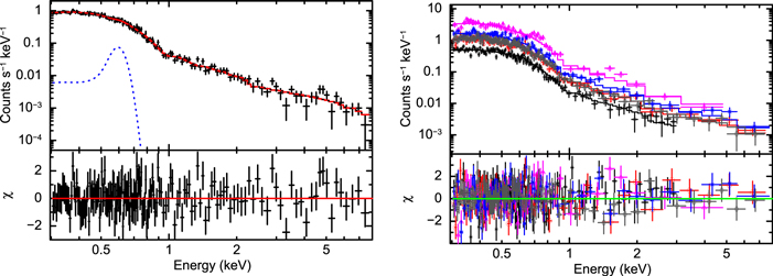
Figure 8. Left: the EPIC-PN mean spectrum, the best-fit absorbed disk Comptonization model, TBabs × WA × (GL+optxagnf), and the deviations of the observed data from the best-fit model. Right: the time-resolved EPIC-PN spectra, the best-fit model, TBabs × WA × (GL+optxagnf), and the residual spectra. The black squares, red circles, magenta triangles, blue crosses, and gray diamonds represent spectral data for Int 1, Int 2, Int 3, Int 4, and Int 5, respectively.
Download figure:
Standard image High-resolution imageTable 2. Best-fit Spectral Model Parameters for the Absorbed Disk Comptonization Model
| Component | Parameter | Average Spectrum | Int 1 | Int 2 | Int 3 | Int 4 | Int 5 |
|---|---|---|---|---|---|---|---|
| 0–38 ks | 38–48 ks | 48–54 ks | 54–60 ks | 60–72 ks | |||
| TBabs |
 (1020 cm−2)a (1020 cm−2)a
|
2.22
|
2.22
|
2.22
|
2.22
|
2.22
|
2.22
|
| WA |
 (1022 cm−2)b (1022 cm−2)b
|

|

|
5.5
|
5.5
|
5.5
|
5.5
|
 /erg cm s−1)c /erg cm s−1)c
|

|

|

|

|

|

|
|
| GL |
 (keV)d (keV)d
|

|

|

|

|

|

|
 (keV)e (keV)e
|

|

|

|

|

|

|
|
| σ (keV)f |

|

|

|

|

|

|
|
 (10−5)g (10−5)g
|

|

|

|

|

|

|
|
| optxagnf |
 ( ( )h )h
|
4.5 
|

|

|

|

|

|
| d (Mpc)i |

|

|

|

|

|

|
|
 j
j
|

|

|

|

|

|

|
|
| ak |

|

|

|

|

|

|
|
 ( ( )l )l
|

|

|

|

|

|

|
|
 (eV)m (eV)m
|

|

|

|

|

|

|
|
| τn |

|

|

|

|

|

|
|
| Γo |

|

|

|

|

|

|
|
 p
p
|

|

|

|

|

|

|
|
 /ν /ν |
154.9/150 | 479.5/404 | ⋯ | ⋯ | ⋯ | ⋯ |
Notes. The absorbed disk Comptonization model is TBabs × WA × (GL+optxagnf), where TBabs = Galactic absorption, WA = warm absorption, GL = Gaussian emission line, optxagnf = disk Comptonized continuum. Parameters with notations ‡ and ∗ denote fixed and tied values, respectively. The notation "p" in error ranges indicates that the confidence limit did not converge.
aColumn density of Galactic neutral hydrogen. bColumn density of the warm absorber (WA). cIonization state of the WA. dRest-frame energy. eObserved-frame energy. fEmission line width. gNormalization in units of photons cm−2 s−1. hSMBH mass. iProper distance. jEddington ratio. kSMBH spin. lCoronal radius. mSoft excess temperature. nOptical depth of the warm corona. oPhoton index of the hot coronal emission. pFraction of the power below that is emitted in the hard Comptonization component.
Download table as: ASCIITypeset image
The soft X-ray excess emission may also arise due to relativistic reflection from an ionized accretion disk (Fabian et al. 2002; Crummy et al. 2006; García et al. 2014). Hence we modeled the soft X-ray excess using the reflection model (reflionx; Ross & Fabian 2005) convolved with the relconv model (García et al. 2014), which blurs the spectrum due to general relativistic effects close to the SMBH. We fitted the 0.3–8 keV EPIC-PN mean spectrum with the thermally Comptonized primary continuum (nthcomp; Zdziarski et al. 1996) and relativistic reflection model (relconv∗reflionx) after correcting for the Galactic absorption (TBabs). The electron temperature of the hot plasma and the temperature of the seed photons in the disk in the nthcomp model were fixed at 100 keV and 50 eV, respectively. The parameters of the reflionx model are iron abundance (AFe), ionization parameter ( , F is the total illuminating flux, n is hydrogen density), normalization (AREF) of the reflected spectrum, and photon index (Γ) of the incident power law. The convolution model relconv has five free parameters: emissivity index (q, where emissivity of the reflected emission is defined by
  ∝ R−q), inner disk radius (Rin), outer disk radius (Rout), black hole spin (a), and disk inclination angle (i). We fixed the outer disk radius at
  . In XSPEC, the 0.3–8 keV model reads as TBabs × (relconv∗reflionx+nthcomp), which provided a reasonably good fit with χ2/dof = 180.8/151. However, the residual spectrum shows an absorption dip at ∼0.9 keV and excess emission at ∼0.6 keV. As before, we fitted the absorption dip with the ionized absorption (WA). The multiplication of the WA model improved the fit statistics to χ2/dof = 165.1/149 (Δχ2 = −15.7 for 2 dof). To model the emission feature at ∼0.6 keV, we added a Gaussian emission line (GL), which provided an improvement in the fit statistics with χ2/dof = 157.1/147 (Δχ2 = −8 for 2 dof). The EPIC-PN mean spectrum, the best-fit absorbed relativistic reflection model, TBabs × WA × (GL+relconv∗reflionx+nthcomp), and the residuals are shown in Figure 9 (left). The best-fit values for the emissivity index, inner disk radius, disk ionization parameter, black hole spin, disk inclination angle, and spectral index of the incident continuum are
  ,
,  ,
,  erg cm s−1,
  ,
,  deg, and
  , respectively. We also fitted the five time-resolved spectra jointly with the absorbed relativistic reflection model and tied every parameter to its mean spectral best-fit value except the normalization (AREF) of the reflection component. This provided an unacceptable fit with χ2/dof = 488.4/404. We then set the normalization (ANTH) of the illuminating continuum to vary between the five spectra and obtained a noticeable improvement in the fitting with χ2/dof = 465.2/399 (Δχ2 = −23.2 for 5 dof). If we let the spectral index (Γ) of the incident continuum vary, we do not get any significant improvement in the fitting. We summarize the best-fit spectral model parameters for both time-averaged and time-resolved spectra in Table 3. The EPIC-PN spectral data sets, the best-fit absorbed relativistic reflection model, and residuals are shown in Figure 9 (right).
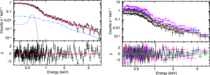
Figure 9. Left: the EPIC-PN mean spectrum, the best-fit absorbed relativistic reflection model (in red), and the deviations of the observed data from the best-fit model, TBabs × WA × (GL+relconv∗reflionx+nthcomp). The primary power-law, relativistic disk reflection and Gaussian emission line components are shown as dashed–dotted, dashed, and dotted lines, respectively. Right: the five time-resolved EPIC-PN spectra, the best-fit model, TBabs × WA × (GL+relconv∗reflionx+nthcomp), and the residual spectra. The black squares, red circles, magenta triangles, blue crosses, and gray diamonds represent spectral data for Int 1, Int 2, Int 3, Int 4, and Int 5, respectively.
Download figure:
Standard image High-resolution imageTable 3. Best-fit Spectral Model Parameters for the Absorbed Relativistic Reflection Model
| Component | Parameter | Average Spectrum | Int 1 | Int 2 | Int 3 | Int 4 | Int 5 |
|---|---|---|---|---|---|---|---|
| 0–38 ks | 38–48 ks | 48–54 ks | 54–60 ks | 60–72 ks | |||
| TBabs |
 (1020 cm−2)a (1020 cm−2)a
|
2.22
|
2.22
|
2.22
|
2.22
|
2.22
|
2.22
|
| WA |
 (1022 cm−2)b (1022 cm−2)b
|

|

|
4.5
|
4.5
|
4.5
|
4.5
|
 /erg cm s−1)c /erg cm s−1)c
|

|

|

|

|

|

|
|
| GL |
 (keV)d (keV)d
|

|

|

|

|

|

|
 (keV)e (keV)e
|

|

|

|

|

|

|
|
| σ (keV)f |

|

|

|

|

|

|
|
 (10−5)g (10−5)g
|

|

|

|

|

|

|
|
| relconv | qh |

|

|

|

|

|

|
| ai |

|

|

|

|

|

|
|
 ( ( )j )j
|

|
1.27
|
1.27
|
1.27
|
1.27
|
1.27
|
|
 ( ( )k )k
|

|
1000
|
1000
|
1000
|
1000
|
1000
|
|
| i (deg)l |

|

|

|

|

|

|
|
| reflionx |
 m
m
|

|

|

|

|

|

|
| Γn |

|

|

|

|

|

|
|
 (erg cm s−1)o (erg cm s−1)o
|

|

|

|

|

|

|
|
 (10−7)p (10−7)p
|

|

|

|

|

|

|
|
| nthcomp | Γq |

|

|

|

|

|

|
 (10−6)r (10−6)r
|

|

|

|

|

|

|
|
 /ν /ν |
157.1/147 | 465.2/399 | ⋯ | ⋯ | ⋯ | ⋯ |
Notes. The absorbed relativistic reflection model is TBabs × WA × (GL+relconv∗reflionx+nthcomp), where TBabs = galactic absorption, WA = warm absorption, GL = Gaussian emission line, relconv∗reflionx = relativistic disk reflection, nthcomp = illuminating continuum. Parameters with notations ‡ and ∗ denote fixed and tied values, respectively. The notation "p" in error ranges indicates that the confidence limit did not converge.
aColumn density of Galactic neutral hydrogen. bColumn density of the warm absorber (WA). cIonization state of the WA. dRest-frame energy. eObserved-frame energy. fEmission line width. gNormalization in units of photons cm−2 s−1. hEmissivity index. iSMBH spin. jInner disk radius. kOuter disk radius. lDisk inclination angle. mIron abundance (solar). nPhoton index of the relativistic reflection component. oDisk ionization parameter. pNormalization of the relativistic reflection component. qPhoton index of the illuminating continuum. rNormalization of the illuminating continuum.Download table as: ASCIITypeset image
5. Flux−Flux Analysis
We perform the flux−flux analysis, which is a model-independent approach to distinguish between the main components responsible for the observed spectral variability and was pioneered by Churazov et al. (2001) and Taylor et al. (2003). Based on our X-ray spectral modeling, we identified the 0.3–1 keV and 1–8 keV energy bands as representatives of the soft X-ray excess and primary power-law emission, respectively. Then, we constructed the 0.3–1 keV versus 1–8 keV flux−flux plot, which is shown in Figure 10 (left). The mean count rates in the soft and hard bands are 0.52 ± 0.04 counts s−1 and 0.08 ± 0.02 counts s−1, respectively. We begin our analysis by fitting the flux−flux plot with a linear relation of the form  , where y and x represent the count rates in the 1–8 keV and 0.3–1 keV bands, respectively. The straight line model provided a statistically unacceptable fit with χ2/dof = 59/32 and implied that the immanent relationship between the soft X-ray excess and primary power-law emission is not linear. Therefore, we fit the flux−flux plot with a power-law plus constant (PLC) model of the form y = αxβ + c (where y and x are as above) following the approach of Kammoun et al. (2015). The PLC model improved the fit statistics to χ2/dof = 37.4/31 and explained the flux−flux plot quite well. We show the best-fit PLC model as the solid line in Figure 10 (left). The best-fit power-law normalization, slope, and constant values are
  counts s−1,
  , and
, and  counts s−1, respectively. The PLC best-fit slope is greater than unity, which indicates the presence of intrinsic variability in the source. The detection of the positive "c"-value in the flux−flux plot implies that there exists a distinct spectral component that is less variable than the primary X-ray continuum and contributes ∼25% of the 1–8 keV count rate at the mean flux level over the observed ∼20 hr timescales. To investigate this issue further, we computed the unabsorbed (without the Galactic and intrinsic absorption) primary continuum and soft X-ray excess flux in the full band (0.3–8 keV) for all five intervals using the XSPEC convolution model cflux and plotted the intrinsic primary power-law flux as a function of the soft X-ray excess flux (the middle panel of Figure 10). The best-fit normalization, slope, and constant parameters, obtained by fitting the FPL versus FBB plot with a PLC model, are
  erg cm−2 s−1,
  , and
, and  erg cm−2 s−1, respectively. Interestingly, we found steeping in the FPL versus FBB plot with an apparent positive constant, which is in agreement with the 0.3–1 keV versus 1–8 keV flux−flux plot. Our flux−flux analysis suggests that the primary power law and soft X-ray excess emission are well correlated with each other, although they vary in a nonlinear fashion on the observed timescale. We also investigated the variability relation between the UV and soft X-ray excess emission in PG 1404+226. Figure 10 (right) shows the variation of the soft X-ray excess flux as a function of the UVW1 flux, which indicates no significant correlation between the UV and soft X-ray excess emission from PG 1404+226.
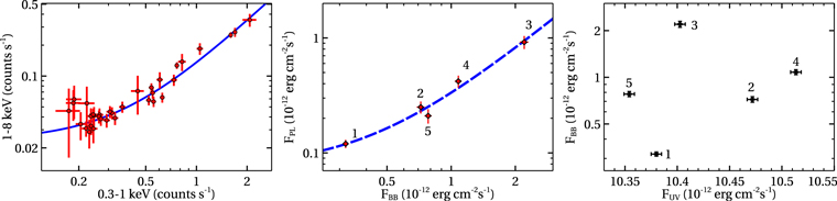
Figure 10. Left: the 1–8 keV count rate is plotted as a function of the 0.3–1 keV count rate with time bins of 2 ks. The solid line represents the best-fit power-law plus constant (PLC) model. Middle: the unabsorbed primary power-law flux vs. blackbody flux in the full band (0.3–8 keV) obtained from five different intervals (marked as 1, 2, 3, 4, and 5). The dashed line shows the best-fit PLC model fitted to the data. Right: the soft X-ray excess flux as a function of the UVW1 flux, implying a lack of correlation between the UV and soft X-ray bands.
Download figure:
Standard image High-resolution image6. Fractional rms Spectral Modeling
To estimate the percentage of variability in the primary power-law continuum and soft X-ray excess emission, and also to quantify the variability relation between them, we derived and modeled the fractional rms variability spectrum of PG 1404+226. First, we extracted the background-subtracted, deadtime-corrected light curves in 19 different energy bands from the simultaneous and equal-length ( ) combined EPIC-PN+MOS data with a time resolution of Δt = 500 s. We have chosen the energy bands so that the minimum average count in each bin is around 20. Then we computed the frequency-averaged (ν ∼ [1.4–100] × 10−5 Hz) fractional rms, Fvar, in each light curve using the method described in Vaughan et al. (2003). We show the derived fractional rms spectrum of PG 1404+226 in Figure 11 (left). The shape of the spectrum is approximately constant with a sharp drop at around 0.6 keV, which can be explained in the framework of a non-variable emission line component at ∼0.6 keV and two variable spectral components: the soft X-ray excess and primary power-law emission, with decreasing relative importance of the soft excess emission and increasing dominance of the primary power-law emission with energy. We constructed fractional rms spectral models using our best-fit phenomenological and physical mean spectral models in ISIS v.1.6.2-40 (Houck & DeNicola 2000).
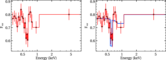
Figure 11. Left: the combined EPIC-PN+MOS, 0.3–8 keV fractional rms spectrum of PG 1404+226. Right: the solid blue line represents the best-fit "two-component phenomenological" model in which the 0.6 keV emission line (GL) is constant, and both the soft X-ray excess (zbbody) and primary power-law emission (zpowerlw) are variable in normalization and positively correlated with each other.
Download figure:
Standard image High-resolution imageFirst, we explored the phenomenological fractional rms spectral model in which the observed 0.6 keV Gaussian emission line (GL) is non-variable, and both the soft X-ray excess (zbbody) and primary power-law emission (zpowerlw) are variable in normalization and correlated with each other. Using Equation (3) of Mallick et al. (2017), we obtained the expression for the fractional rms spectral model:
where  and
and  represent fractional changes in the normalization of the primary power law, fPL, and blackbody, fBB, components respectively. γ measures the correlation or coupling between fPL and fBB. fGL(E) represents the Gaussian emission line component with the observed energy of ∼0.6 keV.
We then fitted the 0.3–8 keV fractional rms spectrum of PG 1404+226 using this "two-component phenomenological" model (Equation (1)) and the best-fit mean spectral model parameters as the input parameters for the above model. This model describes the data reasonably well with χ2/dof = 25/16. The best-fit rms model parameters are  ,
,  , and
, and  . We show the fractional rms variability spectrum and the best-fit "two-component phenomenological" model in Figure 11 (right).
In PG 1404+226, the soft X-ray excess emission was modeled by two different physical models: intrinsic disk Comptonization and relativistic reflection from the ionized accretion disk. To break the degeneracy between these two possible physical scenarios, we constructed fractional rms spectral models considering our best-fit disk Comptonization and relativistic reflection models of the time-averaged spectrum.
In the disk Comptonization scenario, the observed variability in PG 1404+226 was driven by variation in the source luminosity, as inferred from the joint fitting of five EPIC-PN spectra. Therefore, we can write the expression for the fractional rms (see Mallick et al. 2016, 2017) as
where  and
and  represent the best-fit disk Comptonization (optxagnf) and 0.6 keV Gaussian emission line (GL) components, respectively. L is the source luminosity, which is the only variable free parameter in the model. The fitting of the 0.3–8 keV fractional rms spectrum using this model (Equation (2)) resulted in an enhanced variability in the hard band above ∼1 keV with χ2/dof = 32/18. We show the fractional rms variability spectrum and the "one-component disk Comptonization" model in Figure 12 (left).
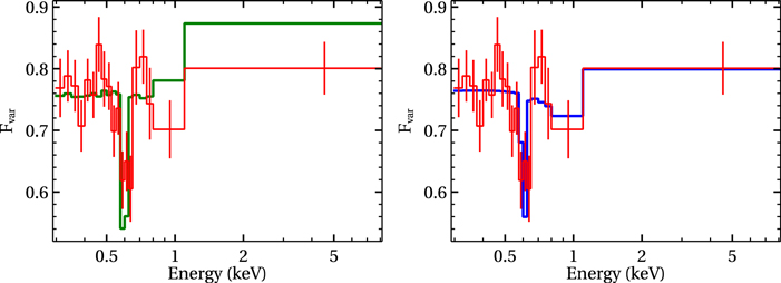
Figure 12. Left: the 0.3–8 keV fractional rms spectrum and the "one-component disk Comptonization" model (solid green) in which the 0.6 keV emission line (GL) is constant and the disk Comptonization (optxagnf) is variable in luminosity only. Right: the 0.3–8 keV fractional rms spectrum and the best-fit "two-component relativistic reflection" model (solid blue) where both inner disk reflection (relconv∗reflionx) and illuminating continuum (nthcomp) are variable in normalization and perfectly correlated with each other. The 0.6 keV emission line (GL) is constant and hence shows a drop in variability at ∼0.6 keV.
Download figure:
Standard image High-resolution imageThen, we investigated the relativistic reflection scenario where the origin of the soft X-ray excess emission was explained with disk irradiation (Crummy et al. 2005). In this scenario, the rapid X-ray variability in PG 1404+226 can be described as a result of changes in the normalization of the illuminating power-law continuum and reflected inner disk emission, as is evident from the time-resolved spectroscopy. Thus, we constructed the "two-component relativistic reflection" model where both the inner disk reflection (relconv∗reflionx) and illuminating continuum (nthcomp) are variable in normalization and perfectly correlated with each other. Mathematically, we can write the expression for the fractional rms as
where
Here  ,
,  , and
, and  represent the best-fit illuminating continuum (nthcomp), inner disk reflection (relconv∗reflionx), and the 0.6 keV Gaussian emission line (GL) components, respectively. The two variable free parameters of this model (Equation (3)) are ANTH and AREF. We then fitted the observed fractional rms spectrum using the "two-component relativistic reflection" model, which describes the data well with χ2/dof = 25/17. We show the fractional rms variability spectrum and the best-fit model in Figure 12 (right). The fractional variations in the normalization of the illuminating continuum and reflected emission are
  and
and  , respectively.
7. Summary and Discussion
We present the first results from our XMM-Newton observation of the NLS1 galaxy PG 1404+226. Here, we investigated the large-amplitude X-ray variability, the origin of the soft X-ray excess emission, and its connection with the intrinsic power-law emission through a detailed analysis of the time-averaged as well as time-resolved X-ray spectra, and frequency-averaged (ν ∼ [1.4–100] × 10−5 Hz) X-ray fractional rms spectrum. Below we summarize our results.
- 1.PG 1404+226 showed a short-term, large-amplitude variability event in which the X-ray (0.3–8 keV) count rate increased exponentially by a factor of ∼7 in about 10 ks and dropped sharply during the 2016 XMM-Newton observation. The hard X-ray (1–8 keV) Chandra/ACIS light curve also showed a rapid variability (a factor of ∼2 in about 5 ks) with an exponential rise and a sharp fall in 2000 (Dasgupta et al. 2005). The rapid X-ray variability had been observed in a few NLS1 galaxies (e.g., NGC 4051: Gierliński & Done 2006; 1H 0707–495: Fabian et al. 2012; Mrk 335: Wilkins et al. 2015). However, the UV (λeff = 2910 Å) emission from PG 1404+226 is much less variable (
 ) than the X-ray (0.3–8 keV) variability ().
 - 2.The source exhibited strong soft X-ray excess emission below ∼1 keV, which was fitted by both the intrinsic disk Comptonization and relativistic reflection models. The EPIC-PN spectral data revealed the presence of a highly ionized (ξ ∼ 600 erg cm s−1) Ne x Lyα absorbing cloud along the line of sight with a column density of NH ∼ 5 × 1022 cm−2 and a possible O viii Lyα emission line. However, we did not detect the presence of any outflow as found by Dasgupta et al. (2005).
- 3.The modeling of the RGS spectrum not only confirms the presence of the Ne x Lyα absorbing cloud and O viii Lyα emission line but also reveals an O viii Lyβ emission line.
- 4.The time-resolved spectroscopy showed a significant variability in both the soft X-ray excess and primary power-law flux, although there were no noticeable variations in the soft X-ray excess temperature ( eV) and photon index of the primary power-law continuum.
- 5.In the disk Comptonization scenario, the rapid X-ray variability can be attributed to a variation in the source luminosity as indicated by the time-resolved spectroscopy. However, the modeling of the X-ray fractional rms spectrum using the "one-component disk Comptonization" model cannot reproduce the observed hard X-ray variability pattern and indicates a reflection origin for the soft X-ray excess emission (see Figure 12, left).
- 6.In the relativistic reflection scenario, the observed large-amplitude X-ray variability was predominantly due to two components: an illuminating continuum and smeared reflected emission; both of them are variable in normalization (see Figure 12, right).
- 7.The inner disk radius and central black hole spin as estimated from the relativistic reflection model are and a > 0.992, respectively. Crummy et al. (2005) also showed that the disk reflection could successfully explain the broadband (0.3–8 keV) spectrum of PG 1404+226 with the radiation from the inner accretion disk around a Kerr black hole. The disk inclination angle estimated from the ionized reflection model is deg, which is in close agreement with that ( deg) obtained by Crummy et al. (2005). The non-detection of the 6.4 keV iron emission line could be due to its smearing on the broad shape in the spectrum.
- 8.We found that the count rates in the soft (0.3–1 keV) and hard (1–8 keV) bands are correlated with each other and vary in a nonlinear manner as suggested by the steepening of the flux–flux plot. The fitting of the hard-versus-soft counts plot with a power-law plus constant (PLC) model reveals a significant positive offset at high energies, which can be interpreted as corroboration for the presence of a less variable reflection component (probably a smeared iron emission line) in the hard band on timescales of ∼20 hr.


7.1. UV/X-Ray Variability and Origin of the Soft X-Ray Excess Emission
The observed UV variability in PG 1404+226 is weak with Fvar ∼ 1% only, whereas the X-ray variability is much stronger (Fvar ∼ 82%) on timescales of ∼73 ks. The UV and soft X-ray excess emission are not significantly correlated as demonstrated in Figure 10 (right).
In the intrinsic disk Comptonization (optxagnf) model, the soft X-ray excess emission results from the Compton up-scattering of the UV seed photons by an optically thick, warm (kTSE ∼ 0.1–0.2 keV) electron plasma in the inner disk (below rcorona) itself. So, if the soft X-ray excess was the direct thermal emission from the inner accretion disk, then we expect correlated UV/soft excess variability. However, we did not find any correlation between the UV flux and X-ray spectral parameters. Furthermore, the modeling of the rms variability spectrum using a "one-component disk Comptonization" model could not describe the observed hard X-ray variability in PG 1404+226 (see Figure 12, left). It might be possible that the UV- and X-ray-emitting regions interact on a timescale much longer than the duration of our observation. To explore that possibility, we calculated various timescales associated with the accretion disk. The light travel time between the central X-ray source and the standard accretion disk is given by the relation (Dewangan et al. 2015)
where  is the scaled mass accretion rate, MBH is the central black hole mass, and λeff is the effective wavelength where the disk emission peaks. In the case of PG 1404+226,
  ,
,  (as obtained from the optxagnf model as well as calculated from the unabsorbed flux in the energy band 0.001–100 keV using the convolution model cflux in XSPEC), and
  for the UVW1 filter. Therefore, the light crossing time between the X-ray source and the disk is ∼13.6 ks, which corresponds to the peak disk emission radius of
  . If we consider a thin disk with a height-to-radius ratio
  (Czerny 2006), the viscous timescale at this emission radius (
 ) is of the order of ∼10 yr, which is much longer than the time span of our XMM-Newton observation. Although both the soft and hard X-ray emission from PG 1404+226 are highly variable, the lack of any strong UV variability is in contradiction with the fluctuation scenario for viscous propagation.
In the relativistic reflection model, the soft X-ray excess is a consequence of disk irradiation by a hot, compact corona close to the black hole. We found a strong correlation between the soft and hard X-ray emission that is expected in the reflection scenario. Additionally, the modeling of the fractional rms spectrum considering a "two-component relativistic reflection" model can reproduce the observed X-ray variability very well (see Figure 12, right).
7.2. Origin of Rapid X-Ray Variability
PG 1404+226 showed a strong X-ray variability with a fractional rms amplitude of  on timescales of ∼20 hr. We attempted to explain the observed rapid variability of PG 1404+226 in the framework of two possible physical scenarios: intrinsic disk Comptonization and relativistic reflection from the ionized accretion disk. In the disk Comptonization scenario, if the rapid X-ray variability is due to the variation in the source luminosity, which is favored by the time-resolved spectroscopy, then it slightly overpredicts the fractional variability in the hard band (see Figure 12, left). Therefore, it is unlikely that the rapid X-ray variability is caused by variations in the luminosity of the source (warm plus hot coronae) only. On the other hand, the soft X-ray excess and primary continuum vary nonlinearly (as
  ), which indicates that the soft X-ray excess is reciprocating with the primary continuum variations, albeit with a smaller amplitude. This is in agreement with the smeared reflection scenario, which is further supported by the high emissivity index (q ∼ 9.9) and non-detection of the iron line. Moreover, the fractional variability spectrum of PG 1404+226 is best described by two components: an illuminating continuum and reflected emission, both of them are variable in flux (see Figure 12, right). We interpret these rapid variations in the framework of the light bending model (Miniutti et al. 2003, 2004; Miniutti & Fabian 2004; Fabian & Vaughan 2005), according to which the primary coronal emission is bent down onto the accretion disk due to strong gravity and forms reflection components including the soft X-ray excess emission. The nature of the rapid X-ray variability in PG 1404+226 favors the "lamppost geometry" for the primary X-ray-emitting hot corona.
L.M. gratefully acknowledges support from the University Grants Commission (UGC), Government of India. The authors thank the anonymous referee for constructive suggestions in improving the quality of the paper. This research has made use of processed data of XMM-Newton observatory through the High Energy Astrophysics Science Archive Research Center Online Service, provided by the NASA Goddard Space Flight Center. This research has made use of the NASA/IPAC Extragalactic Database (NED), which is operated by the Jet Propulsion Laboratory, California Institute of Technology, under contract with NASA. Figures in this manuscript were made with the graphics package pgplot and GUI scientific plotting package veusz.
Facility: XMM-Newton - (EPIC-PN, EPIC-MOS, RGS and OM).
Software: HEASOFT, SAS, XSPEC (Arnaud 1996), XSTAR (Kallman & Bautista 2001), FTOOLS (Blackburn 1995), ISIS (Houck & DeNicola 2000), Python, S-Lang, Veusz, PGPLOT.