


Abstract
We have analyzed a rich, multimission, multiwavelength data set from the black hole X-ray binary (BHXB) LMC X-3, covering a new anomalous low state (ALS), during which the source flux falls to an unprecedentedly low and barely detectable level, and a more normal low state. Simultaneous X-ray and UV/optical monitoring data from Swift are combined with pointed observations from the Rossi X-ray Timing Explorer (RXTE) and X-ray Multi-Mirror Mission (XMM-Newton) and light curves from the Monitor of All-Sky X-ray Image (MAXI) instrument to compare the source characteristics during the ALS with those seen during the normal low state. An XMM-Newton spectrum obtained during the ALS can be modeled using an absorbed power law with  and a luminosity of
  erg s−1 (0.6–5 keV). The Swift X-ray and UV light curves indicate an X-ray lag of ∼8 days as LMC X-3 abruptly exits the ALS, suggesting that changes in the mass accretion rate from the donor drive the X-ray lag. The normal low state displays an asymmetric profile in which the exit occurs more quickly than the entry, with minimum X-ray flux a factor of ∼4300 brighter than during the ALS. The UV brightness of LMC X-3 in the ALS is also fainter and less variable than during normal low states. The existence of repeated ALSs in LMC X-3, as well as a comparison with other BHXBs, implies that it is very close to the transient/persistent X-ray source dividing line. We conclude that LMC X-3 is a transient source that is almost always "on."
Export citation and abstract BibTeX RIS
1. Introduction
LMC X-3 is a bright (up to ∼ in the 0.3–10 keV band pass), high-mass X-ray binary with a 1.7-day orbital period (Cowley et al. 1983). The compact object is a black hole with an estimated mass of
  (Orosz et al. 2014). The spectral type of the optical counterpart is now thought to be a ∼B5 Roche-lobe filling subgiant (Soria et al. 2001). The system displays high-amplitude, long-term variability in the X-ray and ultraviolet, much longer than the orbital period, on the order of 100–300 days. Nowak et al. (2001) analyzed a 100 ks long Rossi X-ray Timing Explorer/Proportional Counter Array (RXTE/PCA) and High Energy X-ray Timing Experiment (HEXTE) observation of LMC X-3 in the high/soft state and detected the source up to 50 keV. The spectrum of the source was well fit by a two-component model of a disk blackbody plus a power law. Wilms et al. (2001) reported strong spectral variability at timescales of days to weeks in a long-term monitoring data set spanning approximately 3 yr from PCA. The same two-component spectral modeling showed luminosity variations of LMC X-3 that scaled with the disk blackbody temperature, with a sharply decreasing temperature and simultaneously harder photon index of ∼1.8 at the lowest count rates. These variations are consistent with state changes exhibited by galactic black hole candidates (Nowak 2006; Dunn et al. 2010; Nowak et al. 2011). Wilms et al. (2001) proposed a wind-driven limit cycle as a mechanism driving the long-term variability.
LMC X-3 is typically observed in the high/soft X-ray spectral state, with an ultrasoft spectrum plus a hard X-ray tail, interspersed with occasional brief low/hard states with a typical duration of 28.7 ± 2.3 days, during which the spectrum can be described using a simple power law (Boyd et al. 2000; Smale & Boyd 2012). However, LMC X-3 has also been observed to undergo two anomalous low states (ALSs), in which the X-ray flux dropped dramatically to a very low level of ∼1 × 1035 erg s−1 (2–10 keV), more than 15 times fainter than the more usual low states, and with durations of 96 and 188 days, respectively, 5–10 times longer than the more usual low states. What causes these extended low states in LMC X-3 is not understood, although they share several characteristics with similar states observed in the canonical precessing accretion disk source Her X-1 (Still & Boyd 2004; Smith et al. 2007).
In LMC X-3, UV emission arises from a variety of locations, including the accretion disk, the ionized stellar wind, the X-ray-illuminated B-star surface, and/or a hot spot on the outer accretion disk. Simultaneous X-ray, optical, and UV observations at a variety of X-ray fluxes help disentangle the various sources of UV radiation. NASA's Swift satellite (Gehrels et al. 2004) is ideal for monitoring LMC X-3 owing to its ability to observe the system in the optical/UV and X-ray simultaneously. Swift observed LMC X-3 in a series of closely spaced observations in 2007, followed by monthly monitoring from 2011 November through 2012 September, and finally a series of observations from 2013 March to 2013 April. This data set includes excellent coverage of a third ALS and a normal low state.
We present an analysis of this data set, supplementing the Swift observations with data from RXTE, the Monitor of All-Sky X-ray Image (MAXI) instrument, and X-ray Multi-Mirror Mission (XMM-Newton). We provide evidence that the X-ray variability lags the optical/UV by ∼8 days, consistent with previous studies (Brocksopp et al. 2001), and presumably governed by the viscous timescale of the accretion disk. This paper is organized as follows: The RXTE, MAXI, Swift, and XMM-Newton observations are presented in Section 2. In Section 3, we describe our results from our light-curve analysis, followed by our spectral analysis. In Section 4 we discuss our findings, and in Section 5 we present our conclusions.
2. Observations
LMC X-3 is a bright, persistent X-ray source in the Large Magellanic Cloud (LMC), a neighboring galaxy located ∼50 kpc away (Pietrzyński et al. 2013), and has been observed for decades by a variety of satellites. Table 1 summarizes all observations discussed here, including start and end times, instruments used, energy ranges, and total observing time. Below, we provide details about the individual data sets, in chronological order.
Table 1. Instrumentation and Observations
| Mission/Instrument | Start Date | End Date | MJD | E-Range | Total Exposure | Number Obs. |
|---|---|---|---|---|---|---|
| (ks) | ||||||
| RXTE/PCA | 2004 Dec | 2012 Jan | 53,340–55,927 | 2–60 keV | 16363.3 | 1273 |
| MAXI | 2009 Jun | 2016 Apr | 54,983–57,508 | 2–30 keV | ∼2082a | 1330 |
| XMM/EPIC | 2011 May | 2012 Jan | 55,682–55,927 | 0.15–15 keV | 48.7 | 4 |
| Swift/UVOT UVW1 | 2011 Nov | 2013 Oct | 55,866–56,566 | 220–400 nm | 11.4 | 20 |
| Swift/UVOT UVW2 | 2011 Nov | 2013 Oct | 55,866–56,566 | 180–260 nm | 35.4 | 46 |
| Swift/UVOT U | 2011 Nov | 2013 Oct | 55,866–56,566 | 300–400 nm | 6.0 | 14 |
| Swift/XRT | 2011 Nov | 2013 Oct | 55,866–56,566 | 0.2–10 keV | 92.6 | 69 |
Note.
aWe use daily averages, each of which has a different effective exposure time, as individual exposure times are not included in the public data release. A typical 1-day exposure time is ∼1565 s, reaching a sensitivity of ∼15 mcrab day–1 in the 2–30 keV band (Sugizaki et al. 2011).Download table as: ASCIITypeset image
2.1. RXTE
The RXTE satellite was launched on 1995 December 30 and was decommissioned in 2012 January 5. It contained three instruments: the All-Sky Monitor (ASM), the PCA, and the HEXTE. The ASM consisted of three wide-angle shadow cameras equipped with proportional counters sensitive to ∼10–20 mCrab day–1 in the 2–10 keV energy range (Levine et al. 1996) and had a collecting area of ∼90 cm2. It provided continuous monitoring of X-ray sources in three different energy bands (1.5–3 keV, 3–5 keV, and 5–12 keV). Its field of view (FOV) was  FWHM (Remillard & Levine 1997) and was able to observe approximately 80% of the sky every 90 minutes with 90 s dwell time. The Crab Nebula and Crab pulsar, a common calibration source for X-ray instruments, produced ∼76 counts s−1 in the ASM.
The PCA consisted of five Xenon proportional counter units (PCUs), which were sensitive to the 2–60 keV energy range, with a collecting area of 6500 cm2 and an FOV at FWHM of 1° (Bradt et al. 1993; Jahoda et al. 1996, 2006). The PCA provided high-sensitivity pointed monitoring observations of LMC X-3, under the Core Program Monitoring proposals 93113, 94113, 95113, and 96113 at a rate of approximately every 3–4 days. The number of proportional counting units operating varied from one observation to the next. Both the Standard1 mode (containing no energy information but at 0.125 s time resolution) and the Standard2 mode (consisting of 129 channels with 16 s time resolution) were used in our analysis.
The HEXTE consisted of two clusters of phoswich scintillation detectors and was sensitive to the energy range of 15–250 keV with a 1° FWHM field of view (Rothschild et al. 1998). Due to the low count rate of the source in HEXTE, these data were not used in our analysis.
The mission ended on 2012 January 5 (MJD 55,931), and data collection ceased at a time when LMC X-3 was apparently entering into its third observed anomalous low state (ALS) as seen in Figure 1. The source was reliably and continuously below 2 counts s−1 PCU−1 beginning approximately 2011 November 20 (MJD 55,885). Then from 2011 December 2 (MJD 55,897), when the source rate was approximately 0.1 counts s−1 PCU−1, the source stayed flat/off through at least the last RXTE observation, taken on 2011 December 28 (MJD 55,923).
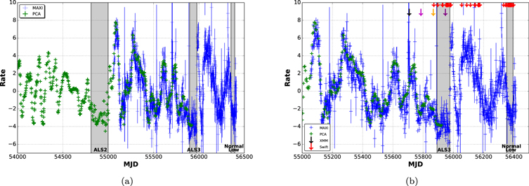
Figure 1. (a) Light curves of LMC X-3 from PCA (green points; 2–60 keV) and MAXI (blue points; 2–30 keV). The mean count rate has been subtracted from each, and they have been normalized to each other such that the maximum and minimum rates are the same. The vertical gray bands denote the times of ALS2, as well as the new anomalous low state reported here (ALS3) and the normal low state we investigate here. (b) Light curves from PCA and MAXI overlaid with arrows indicating the times of Swift (red) and XMM-Newton (black, magenta, orange, and purple) observations have occurred. The vertical gray bands denote the times of ALS3 and the normal low state we investigate here. Clearly, we have excellent coverage of both ALS3 and the normal low state we investigated with MAXI and the Swift pointings. LMC X-3 was also observed with XMM-Newton leading up to ALS3, including one observation inside the ALS.
Download figure:
Standard image High-resolution imageData were obtained through the High Energy Astrophysics Science Archive Research Center (HEASARC) and reduced using standard tools in HEASOFT (Version 6.17) to generate light curves and spectra from standard modes. PCA light curves in separate energy ranges were also obtained from the HEASARC-provided mission-long light curves. To carry out this investigation of ALS3 in the context of the typical long-term variability, it is necessary to construct a single uninterrupted long-term X-ray light curve from a combination of satellites. We can achieve this by scaling MAXI to PCA data (Figure 1).
2.2. MAXI
The MAXI instrument (Matsuoka et al. 2009) is a Japan Aerospace Exploration Agency (JAXA) mission that is operated aboard the International Space Station (ISS). Like the ASM, it is an X-ray all-sky monitor that covers the sky once every ∼96 minutes, collecting X-ray flux measurements for more than 1000 X-ray sources. MAXI consists of both a Gas Slit Camera (GSC) and a Solid-state Slit Camera with combined sensitivity ranging from 0.5 to 30 keV. Project-provided light curves were used. They were created utilizing data from the GSC covering the 2–30 keV energy range and are from the MAXIRIKEN database.4 The GSC has a sensitivity of ∼15 mcrab day–1 (Sugizaki et al. 2011), making MAXI about as sensitive as ASM over a larger energy range. MAXI continuously monitors LMC X-3. There was sufficient overlap in time and energy range that MAXI data can be used in tandem with PCA (Figure 1).
In Figure 1 we display a nearly 7 yr long uninterrupted light curve of LMC X-3, which includes nearly 1000 days of overlap between the PCA and MAXI. The mean count rate has been subtracted from both the PCA and the MAXI light curves (18.83 and 0.06 counts s−1 respectively), and each has been normalized to have the same maximum and minimum value during the overlapping segment. It is clear from Figure 1 that during the time when both the PCA and MAXI were monitoring LMC X-3, the MAXI light curve reproduces essentially all of the variability seen in the PCA. This lends confidence that the MAXI light curve is a faithful tracer of the X-ray variability of LMC X-3 for all times after the end of the RXTE monitoring. The vertical gray bands in Figure 1 indicate the times of ALS2 (MJD 54,811–54,999; Smale & Boyd 2012), as well as the new anomalous low state (ALS3; MJD 55,897–55,975) and the normal low state (MJD 56,353–56,395) we investigate in this paper.
2.3. XMM-Newton
The XMM-Newton satellite (Jansen et al. 2001) was launched in 1999 December. It includes three instruments that operate simultaneously. The Reflection Grating Spectrometers (RGS; den Herder et al. 2001) are diffraction gratings that are coupled to charge coupled device (CCD) detectors. The RGS is sensitive to the 0.33–2.5 keV energy range with a peak effective area of about 150 cm2. The Optical Monitor (OM; Mason et al. 2001) is a 30 cm Ritchey–Chretien telescope on board the spacecraft. The OM covers wavelengths from 170 through 650 nm and samples the 17 arcmin square region of the central X-ray field of view. The European Photon Imaging Camera (EPIC; Strüder et al. 2001; Turner et al. 2001) consists of three cameras, two using metal oxide semi-conductor (MOS) CCDs and one using a pn CCD. EPIC effectively observes the energy range of 0.15–15 keV inside its field of view of 30 arcmin.
Using the EPIC instrument in TIMING mode with MEDIUM filter, XMM-Newton collected a series of four long pointed observations of LMC X-3 to test models of the accretion disk (the MOS cameras were not in use for these observations). The observations began on 2011 May 27 (MJD 55,708) as the source was nearing its last long-term oscillation before ALS3. The first three EPIC observations track the source as it enters ALS3, while the fourth observation occurs in the middle of ALS3 (2012 January 21). In Figure 1 we plot the times of the Swift and EPIC observations along with the light curves from PCA and MAXI. The data were retrieved from the HEASARC archive and reduced in the standard way using SAS Version 13 software, following the method detailed at the ESA website.5 Each data set was reprocessed with the epchain code and filtered with the most stringent conditions ("FLAG==0 && PATTERN<=4") applied.
Light curves were then made and examined. No soft proton contamination (SPC) flares were evident. The spectra and backgrounds for 0671420301, 0671420401, and 0671420501 were then extracted and examined for pileup with the task epatplot. Pileup was seen at low energies; to mitigate this, the boresight column and several columns to either side of it were excised from each observation. This was done in an iterative way, removing a column and checking the modeled and observed single- and double-event pattern distributions until there was good agreement. In the 0671420301 observation, columns with RAWX = 28–48 were extracted, with the central five columns (RAWX = 36–40) removed, leaving 8 × 10⁵ counts in the 0.3–10 keV range. In the 0671420401 and 0671420501 observations, columns with RAWX = 27–47 were extracted, with the central three columns (RAWX = 36–38) removed, leaving 5 × 10⁵ and 5 × 10⁴ counts in the 0.3–10 keV range, respectively. In observations 0671420301, 0671420401, and 0671420501, the fraction of counts removed was 78%, 63%, and 59%, respectively, in the 0.3–10 keV range. The redistribution matrices and ancillary files (RMFs and ARFs) were then made for these three data sets. The ARFs were generated by making the ARF for the entire source extraction region and subtracting from this the ARF for the excised region. For the three bright observations, the background spectra were extracted as far as possible from the boresight (at RAWX = 36, 37, and 38) over the region RAWX = 3–5.
For 0671420601, while no large SPC flares were evident in the light curve, there was low-level contamination throughout the observation. We continued the analysis nonetheless, as the SPC spectrum has been parameterized and can, to some extent, be accounted for in the spectral fitting (Arnaud et al. 2011). No source was visible in this observation, but an attempt was made to see whether any hint of the source might be detected. First, the boresight column had to be determined. To this end, a spectrum from each column between RAWX = 33 and 43 was extracted, and corresponding response files made, over the 0.6–10 keV range. Each was fitted with an absorbed power law, holding the hydrogen column density at the average value within 1° of LMC X-3, 4 × 1020 cm−2 (Kalberla et al. 2005). The resulting best-fit parameters are shown in Figure 2. The RAWX = 38 column has best-fit parameters that are beyond 3σ from the mean of its neighbors. It also has a slightly higher number of photons (140), compared with the other columns (91–125) in this energy range. We therefore took this to be the boresight column and centered the source region on it, extracting RAWX = 35–41. The background region was defined to be the columns on both sides of it, from RAWX = 3–25 and RAWX = 50–62, and the background spectrum and response files were generated.

Figure 2. Best-fit parameters of each column from RAWX = 33 to 43 fitted to an absorbed power law, holding  constant. The solid lines in the top and bottom panels indicate the average value for the background, and the dotted lines correspond to 1 standard deviation about the mean.
Download figure:
Standard image High-resolution image2.4. Swift
The Swift satellite (Gehrels et al. 2004) was launched on 2004 November 20 and includes the co-aligned X-ray Telescope (XRT; Burrows et al. 2005) and Ultraviolet and Optical Telescope (UVOT; Roming et al. 2005), providing simultaneous multiwavelength observations. XRT is an X-ray CCD imaging spectrometer that was designed to locate and study gamma-ray bursts (Cusumano et al. 2006; Vaughan et al. 2006; Evans et al. 2010). It has a 110 cm2 effective area, sensitive to the 0.2–10 keV energy range with an FOV of 23.6 × 23.6 arcmin and an angular resolution of 18 arcsec (Burrows et al. 2005). It observes in a variety of modes, mainly Windowed Timing (WT) or Photon-Counting (PC) mode depending on the count rate observed. The WT mode is a one-dimensional imaging mode with 1.7 ms time resolution, and the PC mode is a two-dimensional imaging mode with 2.5 s time resolution. Both modes have full energy resolution. Our data set includes observations in each mode.
UVOT is a 30 cm aperture ultraviolet and optical telescope using a microchannel plate-intensified CCD detector in a Photon Counting mode (Mason et al. 2004) that is sensitive to magnitude 22.3 in a 1000 s exposure in the white filter. It includes seven broadband filters covering 170–650 nm (Roming et al. 2005), which can be selected by the observer to maximize their science. The FOV is 17 × 17 arcmin, and the camera speed is 11 ms. The flux zero-points of the UVOT data are calibrated as detailed in Breeveld et al. (2011) and Poole et al. (2008).
The Swift satellite has observed LMC X-3 in several campaigns, beginning with seven dedicated pointings in 2007 and continuing with a longer series of monitoring observations beginning in late 2011 for 63 observations. The Swift observations include excellent sampling of ALS3 and the normal low state as shown in Figure 1. See also Table 1 and the Appendix. Spectral fitting was performed using XSPEC Version 12.9.0. Except in the ALS, the data were prepared following the method reported in Evans et al. (2008, 2009) using the XRT products generator,6 which automatically corrects for instrumental artifacts such as pileup; however, no such pileup occurs in our observations. We created spectra using the generated source and background region files, which we read into XSPEC and included the appropriate response and ancillary files (RMF and ARF files). During the ALS observations, the same method was used, except the products were generated manually and a background region consisting of an offset circle (radius of 35.4 arcsec) was subtracted from the WT data. The energy range analyzed was from 0.3 to 10.0 keV, and the data were grouped per observation except for during the ALS. We ignored bad energy channels and subtracted out the background from each observation in the standard way.
3. Analysis
3.1. Light-curve Analysis
In Figure 3, we present the Swift UV and X-ray light curves of LMC X-3, covering ALS3 and a normal low state. Our Swift observations do not provide good coverage of LMC X-3's entrance into the ALS, but they do have excellent coverage of its exit from this state. The observations in early 2013 show that we have complete coverage of the normal low state. To more easily compare our X-ray data sets, we converted into mcrab units using an online tool7 based on Kirsch et al. (2005). We use a distance of 50.6 kpc to derive the luminosity, and all reported errors in this paper are at the 90% confidence level unless otherwise stated. The data were binned to a minimum of 20 counts per bin, allowing for the use of the chi-squared statistic. The exception to this were the data obtained during ALS3, including the Swift WT observations and the XMM-Newton 671420601 observation. Those observations were binned to only require 1 count per bin, and we use the C-statistic (Cash 1979).

Figure 3. (a) Swift light curve from ALS3 until the normal low state we investigated. The upper half of the plot shows the various UVOT (U, UVW1, and UVW2) measurements, while the lower half shows the XRT data (both Window Timing [WT] and Photon Counting [PC] modes) plotted on a logarithmic scale and the same timescale. Data are binned by observation. Plotting the light curves this way easily reveals the time lags between the UV and X-ray variability. (b) Swift light-curve plot showing only ALS3 with data that were binned by observation. As before, the upper half shows UVOT data and the lower half shows the XRT data plotted on the same timescale but centered around ALS3, which allows us to examine more closely LMC X-3's entrance and exit of the ALS. (c) Swift light-curve plot showing the normal low state chosen to be investigated. The upper half shows UVOT data, and the lower half contains the XRT data plotted on the same timescale zoomed in on the normal low state following ALS3 and showing both the entrance and exit from the normal low.
Download figure:
Standard image High-resolution imageWe show the UVOT and XRT light curves of LMC X-3 during ALS3 in Figure 3, where the edges of the gray box mark the beginning and ending of ALS3. Smale & Boyd (2012) defined an ALS as when the X-ray flux drops below ∼ and stays low for 80 days or longer. During this time, the hardness ratio between the 2–4 keV and 4–10 keV bands was always greater than 1. Focusing on the exit from this state, the first observation where XRT was observed to rise out of ALS3 occurred on MJD 55,975.7. In the UVOT light curve, the observations with the UVW1 filter provide the best coverage of the exit. The first of these observations to indicate an increase in flux occurred on MJD 55,967. This implies that the X-rays lag the UV by ∼8 days.
The UVOT and XRT light curves for the normal low state are shown in Figure 3, where again the edges of the gray box mark the beginning and ending of this state. The normal low state was defined by Smale & Boyd (2012) as when the flux fell 1σ below the mean. We have more complete coverage here than we did within the ALS. By fitting the data with a polynomial, we can estimate the model minimum flux and when that occurred in each UVOT filter (U, UVW1, UVW2) and XRT mode (binned by both snapshot and observation). Our results are shown in Table 2. We find that LMC X-3 reaches an X-ray model minimum flux of ∼4.7 ± 2.2 mcrab approximately 24.1 days after the normal low state begins (MJD 56,353). In the UV, the minimum in the model was attained no later than 14.2 days after entrance into the normal low in the UVW1 filter. The measurement is the first observation in the UVW1 filter in the normal low state and is also the lowest flux, implying that the actual time of minimum may have been earlier than this point. For the observations in the U filter, the model minimum occurred 22.6 days after the start of the normal low state, while in the UVW2 filter, it was 23.34 days after entry. The U and UVW1 filters are more sensitive at longer wavelengths, so this is consistent with the X-rays lagging behind the ultraviolet light by ∼1.5–10 days in the normal low state.
Table 2. Time of Minimum Fits during Normal Low
| Measurement | MJD –56,353 | Flux | Error |
|---|---|---|---|
| (erg cm−2 s−1) | |||
| XRT snapshot | 23.15 | 6.04 mcrab | 0.28 |
| XRT obs. | 24.08 | 4.66 mcrab | 2.2 |
| U filter | 22.59 | 9.43E−16 | 2.9E−16 |
| UVW1 filter | 14.22 | 1.36E−15 | 4.7E−17 |
| UVW2 filter | 23.34 | 2.11E−15 | 4.0E−16 |
Download table as: ASCIITypeset image
Next we fit the ALS3 entrance and exit using the MAXI data (see Figure 4 and Table 3) by calculating the rate at which LMC X-3 transitions from high to low flux and vice versa. Our data were converted into mcrab units by using the conversion factor provided in the MAXI documentation.8 We then smoothed the data using a 5-day moving average. It is sufficient to model the entrance and exit of the system in the ALS with a linear fit (Figure 4). The entrance into ALS3 is best modeled with the slope of −0.70 ± 0.12 mcrab day−1 and that of the exit of ALS3 with a slope of 2.17 ± 0.4 mcrab day−1.

Figure 4. (a) MAXI light curve centered on ALS3. This plot shows the MAXI fits of LMC X-3's entrance and exit of ALS3. The MAXI data were averaged into 5-day bins. The slope of the entrance into ALS3 is −0.70 ± 0.12 mcrab day−1, while the slope of the exit from ALS3 is 2.17 ± 0.4 mcrab day−1. (b) MAXI light curve centered on the determined normal low state. This plot shows the MAXI linear fits of the beginning and exit of the normal low. The slope of the normal low entrance was −0.80 ± 0.07 mcrab day−1 and 1.04 ± 0.16 mcrab day−1 for the normal low's exit. We also fit this normal low with a parabola to determine a broad flux minimum estimate of this normal low. This fit estimates that the minimum flux was 1.95 ± 4.82 mcrab occurring on MJD 56,377.76 ± 3.69.
Download figure:
Standard image High-resolution imageTable 3. Entrances and Exits into the Normal Low and ALS
| Normal Low | ALS | |||||
|---|---|---|---|---|---|---|
| Slope (mcrab day−1) | Intercept (day) | Min MJD | Min Flux (mcrab) | Slope (mcrab day−1) | Intercept (day) | |
| MAXI entrance | −0.80 ± 0.07 | 4.48 × 10⁴ ± 3.9 × 10³ | 56,377.76 ± 3.69 | 1.95 ± 4.82 | −0.70 ± 0.12 | 3.92 × 10⁴ ± 6.6 × 10³ |
| MAXI exit | 1.04 ± 0.16 | −5.85 × 10⁴ ± 9.3 × 10³ | 2.17 ± 0.4 | −1.21 × 10⁵ ± 2.2 × 10⁴ | ||
| XRT WT entrance | −1.10 ± 0.09 | 6.22 × 10⁴ ± 5.2 × 10³ | 56,378.70 ± 1.67 | 5.89 ± 2.15 | ⋯ | ⋯ |
| XRT WT exit | 1.46 ± 0.15 | −8.24 × 10⁴ ± 8.4 × 10³ | 18.69 ± 2.82 | −1.05 × 10⁶ ± 1.58 × 10⁵ |
Download table as: ASCIITypeset image
Using the same procedure as above, we fit the normal low state entrance and exit. We consider MJD 56,350–56,406 for a typical normal low state. We again find that a linear fit models the behavior reasonably (Figure 4 and Table 3). The slope of the system for the best model of the entrance to the normal low state was −0.80 ± 0.07 mcrab day−1 and 1.04 ± 0.16 mcrab day−1 for the exit. We also fit all data from the normal low (MJD 56,350–56,406) to a polynomial in order to estimate a broad flux minimum of the model. We found that the flux minimum was 1.95 ± 4.82 mcrab occurring on MJD 56,377.76 ± 3.69. This corresponds to a luminosity of ∼2 × 1037 erg s−1 in the 2–20 keV band.
With Swift we do not have good coverage of the entrance into ALS3, but its exit from ALS3 is reasonably fit with a linear model. We required the fit to pass through the first significant detection after ALS3 in order to measure the initial rise, which is best modeled with a slope of 18.69 ± 2.82 mcrab day−1 for the WT data. From the X-intercept, we estimate that LMC X-3 began its exit from ALS3 on MJD 55,975.3. This is shown in Figure 5 and Table 3. The Swift data have excellent coverage of the same normal low state, including both the entrance into and exit from this state as can be seen in Figure 5 and Table 3. The slope of the entrance was −1.10 ± 0.09 mcrab day−1 in the WT data, and the slope of the exit was 1.46 ± 0.15 mcrab day−1. As in the MAXI data, we estimated the model flux minimum to be 5.89 ± 2.15 mcrab occurring on MJD 56,378.70 ± 1.67, corresponding to a luminosity of ∼9 × 1037 erg s−1 in the 0.3–10 keV band. Together, the MAXI and Swift estimates of the normal low's parameters are compatible within the estimated error.
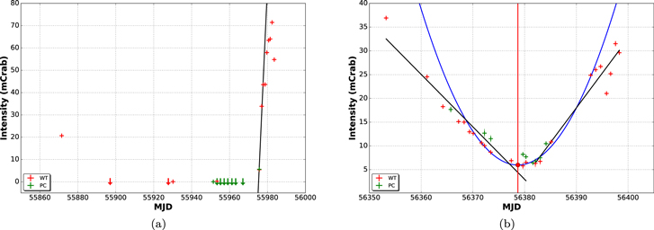
Figure 5. (a) XRT light curve during the ALS3. There is not full coverage of the ALS3 with Swift, but we do have good coverage of the exit from this state as shown. We required the fit to pass through the first significant detection. The initial rise of the exit is best modeled with the slope of 18.69 mcrab day−1 in the WT data. From the X-intercept, we estimate that LMC X-3 began to exit the ALS on MJD 55,975.3. (b) XRT light curve during the determined normal low state. Unlike ALS3, we have excellent coverage of the entire normal low state with Swift. We include on this plot the XRT fits of the normal low entrances and exits. The slope of the entrance was −1.10 mcrab day−1 in the WT data and exited at a rate of 1.46 mcrab day−1. Fitting these data with a polynomial yields a minimum flux of 5.89 ± 2.15 mcrab occurring on MJD 56,378.70 ± 1.67.
Download figure:
Standard image High-resolution image3.2. Spectral Analysis
3.2.1. Swift/XRT
We fit the XRT spectrum while LMC X-3 was in an ALS state, and for each observation when it was in a typical normal low state. A sample XRT spectrum from a typical state, as well as a normal low state, is shown in Figure 6. We examined three different models in our analysis: a disk blackbody, a power law, and a combination of these. We found that the combination model typically provided the best fit and with a value of reduced  . We used the absorption component TBABS, and our complete model was tbabs × (diskbb + powerlaw). The data that were fitted for the normal state are from observation 00045613010, which occurred on 2012 August 26 (MJD 56,165). We then fit the data and obtained a reduced
  of 1.12 with 678 degrees of freedom. We found that the best fit had parameters of neutral hydrogen column density
  cm−2, disk temperature
  keV with a normalization of
  , and a photon index
  with normalization of
  . Our model had a derived luminosity of
  erg s−1 in the 0.3–10 keV band at 50.6 kpc. We can cross-reference our value for
  with the Leiden/Argentine/Bonn (Kalberla et al. 2005) and Dickey & Lockman (Dickey & Lockman 1990) surveys of the Galactic H i column density available on HEASARC, which found that
  cm−2 and
  cm−2, respectively, which is just slightly lower than our value.
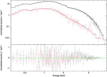
Figure 6. Example XRT spectrum from an observation during a normal low state (red) and during a typical state (black). The residuals of the best-fit model, a disk blackbody with a power law, are shown.
Download figure:
Standard image High-resolution imageA typical normal low flux state is also shown in Figure 6. These data were fitted from observation 00045613026, which were obtained on 2013 March 26 (MJD 56,377). We followed the same procedure as above to fit the data and obtained a reduced  of 1.11 with 526 degrees of freedom. We found that the best fit had the following parameters:
  of
of  cm−2,
cm−2,  of
of  keV with a normalization of
  , and a Γ of
  with normalization of
  . Our model had a derived a luminosity of
  erg s−1 in the 0.3–10 keV band at 50.6 kpc.
The parameters obtained for this and other observations are collected in Table 4. Flux measurement of the model parameters during ALS3 was found by combining all observations that occurred during this period using xselect. These observations (total exposure of 1.4 ks in the WT mode) had to be combined because the system is so dim (below ∼2 × 1035 erg s−1) that our model cannot yield physical results otherwise. There are additional observations in the PC mode; however, even combined, they were too faint for analysis. Additionally, during ALS3 we fit the data with a pure power-law model with the neutral hydrogen column density frozen at  cm−2, consistent with radio measurements and from the O i edge (Nowak et al. 2001; Page et al. 2003; Smith et al. 2007). Our fit yielded a reduced cstat of 1.38 with 18 degrees of freedom and a photon index of
  with a normalization of 1 × 10⁻⁴.
Table 4. Disk Blackbody and Power-law Model Parameters of Normal Low State and ALS
| MJD | NH | Tin | NT | Γ | NΓ | Reduced 
|
dof | Flux | Flux DiskBB | Flux Power Law | Exp Time | Rate | Rate Err |
|---|---|---|---|---|---|---|---|---|---|---|---|---|---|
| −56,345.61 | (1022) | (keV) | (erg cm−2 s−1) | (erg cm−2 s−1) | (erg cm−2 s−1) | (s) | (counts s−1) | (counts s−1) | |||||
| ALS WT | 0.04 | ⋯ | ⋯ |

|

|
1.38a | 18 | 5.4E−13 | ⋯ | 5.4E−13 | 1374 | 2.3E−2 | 1.2E−2 |
| 0 |

|

|

|

|

|
1.34 | 716 | 1.37E−9 | 1.11E−9 | 2.56E−10 | 2153 | 20.5 | 0.1 |
| 7.61 |

|

|

|

|

|
1.46 | 676 | 6.84E−10 | 5.47E−10 | 1.37E−10 | 1609 | 20.2 | 0.11 |
| 15.51 |

|

|

|

|

|
1.20 | 551 | 4.68E−10 | 4.16E−10 | 5.25E−11 | 646.4 | 15.6 | 0.16 |
| 18.6 |

|

|

|

|

|
1.25 | 596 | 3.47E−10 | 2.69E−10 | 7.79E−11 | 1450 | 12.2 | 0.09 |
| 20.1 |

|

|

|

|

|
1.14 | 288 | 2.99E−10 | 1.72E−10 | 1.26E−10 | 494.5 | 1.72 | 0.06 |
| 21.61 |

|

|

|

|

|
1.11 | 462 | 2.72E−10 | 1.99E−10 | 7.27E−11 | 492.8 | 9.84 | 0.14 |
| 22.68 |

|

|

|

|

|
1.05 | 454 | 2.71E−10 | 2.04E−10 | 6.70E−11 | 488.4 | 9.77 | 0.15 |
| 23.73 |

|

|

|

|

|
1.16 | 563 | 2.43E−10 | 1.79E−10 | 6.42E−11 | 2221 | 7.88 | 0.06 |
| 24.44 |

|

|

|

|

|
1.21 | 443 | 2.28E−10 | 1.68E−10 | 5.99E−11 | 548.9 | 8.33 | 0.13 |
| 26.03 |

|

|

|

|

|
1.10 | 421 | 1.85E−10 | 9.30E−11 | 9.17E−11 | 578.2 | 7.05 | 0.11 |
| 26.62 |

|

|

|

|

|
1.08 | 386 | 1.82E−10 | 1.06E−10 | 7.60E−11 | 354.7 | 6.69 | 0.14 |
| 27.83 |

|

|

|

|

|
1.11 | 344 | 1.54E−10 | 7.51E−11 | 7.92E−11 | 311 | 5.70 | 0.14 |
| 31.8 |

|

|

|

|

|
1.11 | 526 | 1.25E−10 | 5.33E−11 | 7.13E−11 | 1962 | 4.66 | 0.05 |
| 34.04 |

|

|

|

|

|
1.46 | 248 | 1.12E−10 | 2.43E−11 | 8.81E−11 | 594.4 | 1.21 | 0.05 |
| 34.64 |

|

|

|

|

|
0.85 | 217 | 1.15E−10 | 3.31E−11 | 8.19E−11 | 469.5 | 1.00 | 0.05 |
| 35.98 |

|

|

|

|

|
1.15 | 243 | 1.14E−10 | 5.28E−11 | 6.12E−11 | 606.8 | 1.14 | 0.04 |
| 36.45 |

|

|

|

|

|
1.14 | 238 | 1.08E−10 | 5.48E−11 | 5.30E−11 | 541.9 | 1.15 | 0.05 |
| 37.38 |

|

|

|

|

|
1.19 | 206 | 1.11E−10 | 6.17E−11 | 4.87E−11 | 364.6 | 1.20 | 0.06 |
| 38.52 |

|

|

|

|

|
1.45 | 257 | 1.68E−10 | 4.78E−11 | 1.20E−10 | 601.9 | 1.17 | 0.04 |
| 39.51 |

|

|

|

|

|
1.03 | 544 | 1.95E−10 | 1.66E−10 | 2.89E−11 | 2104 | 7.22 | 0.06 |
| 47.14 |

|

|

|

|

|
1.38 | 586 | 4.81E−10 | 4.24E−10 | 5.63E−11 | 984.8 | 16.48 | 0.13 |
| 48.11 |

|

|

|

|

|
1.22 | 578 | 5.04E−10 | 4.49E−10 | 5.52E−11 | 872.9 | 16.2 | 0.14 |
Note.
aThis is the reduced cstat value, and there are only 32 counts in the source.Download table as: ASCIITypeset image
We also derived the total flux and the component fluxes of our observations (included in Table 4) tracking LMC X-3 throughout the normal low state. This was done using the absorbed flux in the 0.3–10 keV band. Changes in the component flux contribution track the change in total flux throughout the normal low state. The disk contribution is the primary component of the total flux and is ∼4× larger than the contribution from the power law in the brightest observation. The disk contribution drives the change in the total flux, while the flux from the power law remains relatively constant. The flux in the disk decreases until it is approximately equal to the flux in the power-law component, which occurs at the minimum of the normal low state. The disk flux then increases to pre-normal low levels. This is consistent with possible changes in the size or orientation of the disk.
3.2.2. XMM-Newton
LMC X-3 was observed with XMM-Newton for four observations, three that tracked the entrance into ALS3 and one observation entirely within ALS3 (observations shown in Figure 1). After preparing the data as described in Section 2, we again used XSPEC to fit the spectra. We show our results in Table 5 and plot the spectral fits of our four observations in Figure 7.
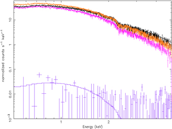
Figure 7. Spectral fits from XMM data, tracking LMC X-3 as it enters ALS3. The first observation is shown in black, the second in magenta, the third in orange, and the fourth observation, occurring in ALS3, is shown in purple. The flux in the fourth observation is more than three orders of magnitude lower than those in the previous observations.
Download figure:
Standard image High-resolution imageTable 5. XMM-EPIC Fits
| XMM ObsID | 671420301 | 671420401 | 671420501 | 671420601 | Units |
|---|---|---|---|---|---|
| Date | 2011 May 27 | 2011 Aug 12 | 2011 Nov 2 | 2012 Jan 21 | ⋯ |
| MJD | 55,708 | 55,785 | 55,867 | 55,939 | ⋯ |
| Exposure time | 12.9 | 11.9 | 11.9 | 11.9 | ks |
| EPIC ratea | 67.2 ± 0.1 | 50.3 ± 0.1 | 69.9 ± 0.1 | 7.2E−2 ± 2.6E−3 | counts s−1 |
| NH | 0.13 ± 0.03 | 0.13 ± 0.01 | 0.12 ± 0.01 | 0.04b | 1022 cm−2 |
| Γ | 2.69 ± 0.2 | 2.98 ± 0.08 | 2.90 ± 0.07 | 1.41 ± 0.65 | ⋯ |
| NΓ | 0.077 ± 0.01 | 0.034 ± 0.002 | 0.046 ± 0.003 | (5.35 ± 1.85) × 10−6 | ⋯ |
| Tin | 1.27 ± 0.02 | 0.88 ± 0.01 | 0.97 ± 0.01 | ⋯ | keV |
| NT | 11.69 ± 0.8 | 18.45 ± 0.9 | 18.44 ± 0.7 | ⋯ | ⋯ |
Red 
|
1.08 | 1.01 | 1.00 | 1.05c | ⋯ |
| Fluxd | 7.91E−10 | 2.76E−10 | 4.08E−10 | 2.6E−14 | erg cm−2 s−1 |
| XMM luminosityd | 2.49E+38 | 8.68E+37 | 1.28E+38 | 7.97E+33 | erg s−1 |
| L/LEdde | 2.71E−01 | 9.43E−02 | 1.04E−01 | 9.25E−06 | ⋯ |
| Fluxf | 4.42E−10 | 1.12E−10 | 1.82E−10 | ⋯ | erg cm−2 s−1 |
| RXTE ObsID | 96113-01-42-00 | 96113-01-64-00 | 96113-01-88-00 | None | ⋯ |
| RXTE date | 26 May 2011 | 11 Aug 2011 | 2 Nov 2011 | None | ⋯ |
| RXTE MJD | 55,707 | 55,785 | 55,867 | ⋯ | ⋯ |
| RXTE exposure time | 1.9 | 1.6 | 1.9 | ⋯ | ks |
| RXTE fluxg | 4.94E−10 | 1.27E−10 | 2.01E−10 | ⋯ | erg cm−2 s−1 |
| RXTE rate | 38.11 | 9.67 | 14.19 | ⋯ | counts s−1 PCU−1 |
Notes.
aRate from the extracted source region and over the energy range of 0.3–10 keV for the first three observations and 0.6–5 keV for the 671420601 observation. bFixed to be consistent with Nowak et al. (2001), Page et al. (2003), and Smith et al. (2007). cThis is the reduced cstat value. dAbsorbed flux/luminosity over the range of 0.3–10 keV for the first three observations and 0.6–5 keV for the 671420601 observation. eLEdd represents the Eddington luminosity, which is the maximum luminosity attainable by a stellar object that is in hydrostatic equilibrium. fAbsorbed flux over the range of 2–10 keV for comparison with RXTE fluxes. gAbsorbed flux over the range of 2–10 keV.Download table as: ASCIITypeset image
As with XRT, the spectra are modeled as an absorbed disk blackbody with a power-law component. Our results are presented in Table 5. The first observation (0671420301, shown in black in Figure 7) has a fairly typical fit, with a photon index of Γ = 2.69 ± 0.2 and a disk temperature of about 1.27 keV. The fits to the next two observations (magenta and orange, respectively) show that the system drops in overall flux and displays a softer spectrum.
The last observation (0671420601, shown in purple) illustrates how dramatically different the system is during the ALS. For this observation, our spectra can be modeled by a simple power law. LMC X-3 dims by a factor of more than ∼16,000 in just 72 days, and the disk component becomes unnecessary.
The first three XMM observations occurred before PCA monitoring ceased. Fortunately, for each of these three observations, there are PCA data taken within 24 hr of the XMM observation. To check the reliability of our spectral fitting parameters of the EPIC timing data, we extracted the STD2 spectra from each of these PCA observations and fit them with the same two-component model. These results are included in Table 5. In all three cases, the flux derived from the modeled RXTE spectra differs from the flux derived from the EPIC TIMING mode spectra by less than 13% when restricted to the same energy range, lending additional confidence to our XMM flux measurements, particularly for the fourth and final observation during ALS3.
For the 671420601 data set, we first analyzed the background spectrum. In addition to the expected SPC (see Section 2.3), which manifested as a shallow-sloped power law, contamination from solar wind charge exchange (SWCX) was evident as strong emission lines at  . Fluorescent instrumental lines from Al (∼1.5 keV) and Cu (8–10 keV) were visible.
Before fitting the background spectrum, we needed reasonable initial values for the parameters and constraints for the models at low energies. To this end, we obtained ROSAT All-Sky Survey (RASS) data in an annulus between 0.5° and 1.0° around the source9
and fitted the background spectrum with the "xspec-sxrbg.tcl" script in XSPEC10
(Arnaud et al. 2011). This modeled the background spectrum as an absorbed power law and thermal plasma emission, with an additional (unabsorbed) plasma emission component: abs × (powerlaw + apec) + apec. Physically, the power law corresponds to unresolved active galactic nuclei, while the absorbed and unabsorbed plasma emission corresponds to the Galactic hot halo and Local Hot Bubble, respectively. The photon index was held at 1.45 (Chen et al. 1997), and  was held at 4 × 1020 cm−2 (Kalberla et al. 2005). This yielded plasma temperatures of ∼0.1 and 0.2 keV for the two apec components, as is expected for the Local Hot Bubble and hot halo (Arnaud et al. 2011).
The XMM background spectrum was then fit using cstat statistics in Sherpa (CIAO v. 4.7) with the same model, plus components to account for the instrumental, SWCX, and soft proton contributions. This was done in several steps, starting with fitting the continuum without the instrumental lines and SWCX contributions (i.e., abs × (powerlaw+ apec) + apec + powerlaw, where the unabsorbed power law models the SPC) over the ranges E = 0.3–0.4 keV, 0.6–1.4 keV, 1.7–7 keV, and 10–11 keV. The photon index and temperatures from the RASS fit were frozen, with the normalizations and the unabsorbed power-law parameters allowed to float. Then, a Gaussian at 1.5 keV was added to account for the instrumental Al Kα, and two more Gaussians were added to account for the SWCX lines near 0.45 keV, and the spectrum was fitted in the ranges 0.4–7 keV and 10–15 keV. Then, we fitted the instrumental lines at higher energies. It is generally recommended that five Gaussians be used for these lines,11 but not all were resolved. We began by adding five, with the line energies set initially at 7.1, 7.5, 8.1, 8.6, and 8.9 keV, but found that this produced a "line" with a normalization of 0. Two Gaussians were removed and the background spectrum was refit, which produced physically realistic parameters for all model components. Finally, with other components fit reasonably well, the power law and temperatures from the RASS fit were allowed to float. The best-fit parameters from the final fit, over the range 0.4–11 keV, and the estimate of goodness of fit are listed in Table 6.
Table 6. Background Fitting Results for the 0671420601 Data Set
| Fit Parametera | Value |
|---|---|

|
0.04 |

|
0.24 ± 0.24 |

|
1.21 ± 0.41 |

|
0.12 ± 0.06 |

|
0.19 ± 0.05 |
| Gaussian 1: line energy | 0.456 ± 0.001 |
| Gaussian 1: line width | 0.010 ± 0.001 |
| Gaussian 2: line energy | 0.476 ± 0.004 |
| Gaussian 2: line width | 0.020 ± 0.002 |
| Gaussian 3: line energy | 1.55 ± 0.02 |
| Gaussian 3: line width | 0.08 ± 0.02 |
| Gaussian 4: line energy | 8.05 ± 0.21 |
| Gaussian 4: line width | 0.18 ± 0.14 |
| Gaussian 5: line energy | 8.49 ± 0.06 |
| Gaussian 5: line width | 0.15 ± 0.04 |
| Gaussian 6: line energy | 9.21 ± 0.06 |
| Gaussian 6: line width | 0.20 ± 0.06 |
| Cstat/dof | 3330.46/2900 |
Note.
aNH was frozen for all fits and is in units of 1022 cm−2. Plasma temperatures kT, line energies, and line widths are in keV.Download table as: ASCIITypeset image
Once the background was parameterized, we turned our attention to the source. The source was modeled as an absorbed power law, holding Galactic  frozen at 4 × 1020cm−2 and using zvfeabs to model absorption in the LMC and within the system itself (Wu et al. 2001), with the iron and total metal abundances set to 40% solar (Caputo et al. 1999). The standard method for such low-count spectra is to fit the background and source simultaneously, but this resulted in unphysical fit parameters, so all background parameters were frozen. We could not detect LMC absorption, so we refit the spectrum with Galactic absorption only; over the range 0.6–5 keV, this yielded photon index Γ = 1.41 ± 0.65, normalization = (5.35 ± 1.85) × 10−6, flux = 2.6 × 10⁻¹⁴ erg cm−2 s−1,
  erg s−1, and cstat/dof = 1860.9/1772. We calculated this to be a 1.83σ upper limit on the flux and note that if this is a marginal detection then this flux is very close to those of galactic black hole binaries in quiescence (
 erg s−1 or
  Plotkin et al. 2013).
As was also seen by Wu et al. (2001) and attributed to possible systematic effects, the  values in our spectral fits sometimes are significantly higher than the Galactic
  . We consider the possibility suggested by Miller et al. (2009) that the column density in individual photoelectric absorption edges is constant with luminosity. To test whether unphysical
  values would substantially change our model parameters, we recalculated the spectral models for the first three XMM observations with
  fixed at 4 × 1020cm−2. For example, for the 6171420301 observation, our new parameters were Γ = 2.20 ± 0.06 (∼18% decrease, ∼2.4σ), NΓ = 0.04 ± 0.002 (∼44% decrease, ∼3.7σ), Tin = 1.21 ± 0.01 keV (∼5% decrease, ∼3σ), NT = 14.54 ± 0.56 (∼24% increase, ∼3.6σ), red χ2 = 1.09 (∼1.5% increase), flux = 8.05 × 10⁻¹⁰ erg cm−2 s−1 (<2% increase), and luminosity = 2.53 × 1038 erg s−1 (<2% increase). With
  fixed, the primary changes in our model are that the normalizations change significantly while the other parameters change to a lesser degree. We also fit these observations with the models simpl, compTT, and Nthcomp, but none of these models provided a significant improvement to the fit, and they only had a minor effect on disk parameters. One caveat to the argument noted by Miller et al. (2009) is that it may not hold for X-ray binaries that are "dippers" or when there are winds from massive stars. We cannot rule out that our
  values could potentially be due to the large accretion disk that may be tilted or warped and that the changing geometry could be causing variations in the column density.
4. Discussion
LMC X-3 is an unusual system in that it exhibits complex long-term variability on timescales of 100–300 days, as well as anomalous low states of at least 80 days. The source has now been observed in such an ALS on three separate occasions: 2003 December through 2004 March (ALS1; Smale & Boyd 2012), 2008 December through 2009 June (ALS2; Smale & Boyd 2012), and 2011 December through 2012 February (ALS3; this paper). During an ALS, the spectrum can be fit by a simple, hard, power-law model, and the source flux drops by approximately three orders of magnitude. Using data from MAXI, Swift, and XMM, we have studied ALS3 in detail and compared its properties to a more normal low state. We have also fit the entrances and exits from each state in the light curve. Our findings are presented below.
4.1. Comparison of an ALS and Normal Low State
In terms of its spectrum and flux decrease, the properties of ALS3 are similar to those of ALS1 and ALS2. The duration of ALS3 is slightly shorter than that of the earlier events, with a duration of 80 days, whereas ALS1 and ALS2 lasted 96 and 188 days, respectively. All the ALSs are significantly longer in duration than the typical low states in LMC X-3, which have an average duration of 28.7 ± 2.3 days (Smale & Boyd 2012). All three ALSs reach a similar low flux ≤∼1035 erg s−1, as compared to ∼1038 erg s−1 in a typical high state.
Our comparison of the system's characteristics during ALS3 and the normal low state can yield insights into the mechanisms that drive X-ray and UV variability. While the difference in minimum X-ray count rate between ALS3 and the normal low state is obvious in Figure 3, as well as the Appendix, it is instructive to consider the difference in minimum UV flux for the same time spans. The flux reaches a minimum of  erg cm−2 s−1 in UVW1 on MJD 55,963 in the ALS. If, during this time, the contributions from an accretion disk, hot spot, and reprocessing from the companion had dropped to essentially zero, then the ALS flux represents the UV contribution from the B star alone. On MJD 56,367, in the normal low state, the minimum flux in the UVW1 filter is about 1.4 times greater than the B star alone (i.e., ∼40% brighter), at
  erg cm−2 s−1, while the flux in UVW1 for a typical X-ray rate (MJD 56,055) is
  erg cm−2 s−1, or about 3.6 times greater than B star ALS flux (∼260% brighter). Similarly, for the UVW2 filter, the flux reaches a minimum of ∼
 erg cm−2 s−1 (averaging values from MJD 55,930 to 55,961) during the ALS, while in the normal low state (MJD 56,373–56,381) it is
  erg cm−2 s−1 (∼1.3 times greater than the B star, or ∼30% brighter), and during a typical X-ray flux (MJD 56,141–56,145) it is
  erg cm−2 s−1 (∼2.4 times greater than the B star flux, or ∼140% brighter). In other words, if this additional UV light is assumed to be from the accretion disk only, then during a normal low, ∼70%–80% of the UV light is due to the star, while at more typical X-ray brightnesses, only ∼30%–40% of the UV light is from the star. By contrast, Steiner et al. (2014) found that about 80% of the optical through infrared (OIR) flux of LMC X-3 is due to the star, throughout its range of X-ray variability. They also found that the X-ray flux lagged the OIR flux by a roughly constant ∼15–16 days and is possibly weakly dependent on flux. Combining the Steiner et al. (2014) results with ours suggests that the disk is significantly brighter with respect to the companion in the UV than in the OIR; the difference in measured lag between optical (16 days) and UV (∼8 days) implies that the location of the UV ring in the disk is interior to the OIR source. Further study of the UV brightness will be presented in a future paper (Torpin et al. 2017b, in preparation).
If this additional UV variability is due to the accretion disk, one possible explanation is that the disk may be warped, tilting, and chaotically precessing. Ogilvie & Dubus (2001) showed that the radiation-driven warping instability of accretion disks in X-ray binaries produces steadily precessing disks only in a small region of parameter space close to the stability limit. They postulated that systems farther from the stability limit could show quasi-periodic or chaotic precession. This case was strengthened by analysis of several long-term variability systems by Clarkson et al. (2003), which showed evidence that several systems appeared to precess in a combination of warping modes. Smale & Boyd (2012) found that the nonperiodic long-term variability of LMC X-3 exhibited several characteristics of a nonlinear oscillator. While such a model may explain some characteristics of the variability, this explanation appears unlikely. LMC X-3 has an inclination angle of ∼70° (Orosz et al. 2014) and a subgiant companion. There is no evidence of any eclipsing in the long-term light curves, and this imposes a significant constraint on the size of any warp or tilt. Foulkes et al. (2010) found in their simulations that LMC X-3 had a likely tilt of ∼10° and a maximum warp of ∼20° located at the disk edge. This will add some variability, but it is unlikely that such a warp and tilt would be responsible for the entirety of the additional UV flux observed.
Another possible explanation for this variability is strong stellar wind in the system; however, this is also improbable. Wu et al. (2001) and Soria et al. (2001) in their analysis of XMM-Newton observations of LMC X-3 found that a strong stellar wind could not be supported. In particular, Wu et al. (2001) measured column densities of  cm−2, which is in good agreement with our results and is too small to suggest the presence of such a wind. It should be noted, however, that they were unable to determine whether their
  variations are correlated with the X-ray luminosity. Our XMM-Newton observations do show absorption values increasing slightly through the ingress of ALS3, which may hint at the existence of a possible accretion stream. Additionally, Cambier & Smith (2013) and Proga (2003) found through modeling that a stellar wind is unlikely to contribute significantly to the variability. Further evidence arises from examining the Swift hardness ratio and the X-ray count rate within the normal low state as shown in Figure 8. We find a positive Pearson correlation coefficient of r = 0.72 between the two, which argues against the existence of a strong wind, as it could deplete the amount of accreting gas and result in reduced X-ray emission (Apparao & Tarafdar 1992). The energy bands used for the hardness ratio were 0.3–1.5 keV for the soft band and 1.5–10 keV for the hard band and are given in the Appendix.

Figure 8. Swift hardness ratio vs. Swift count rate within the normal low state. The red line is the best linear fit to the data, and we find a Pearson correlation coefficient of r = 0.72.
Download figure:
Standard image High-resolution imagePerhaps a more likely explanation of this variability is that there is a change in the mass accretion rate from Roche lobe overflow. Cambier & Smith (2013) studied the effect of supply rate modulation in their model of the accretion flow variability in LMC X-3 and found it significant but unable to explain the variability by itself. Additionally, Cambier & Smith (2013) included the effects of disk bifurcation at the edge of the disk, Compton-heated winds, and partial hydrogen ionization instability and also considered the effect of evaporation and condensation, but they are unable to definitively explain LMC X-3's behavior at present. Most likely, some combination of these mechanisms (stellar wind, disk warping, mass accretion rate changes) drives the variability of LMC X-3.
The X-ray flux exhibits even more interesting behavior. The measured XRT count rate during our ALS monitoring drops such that it is indistinguishable from the background prior to flaring (∼0.02 counts s−1). While LMC X-3 is in its normal low state, the X-ray count rate is ∼1.1 counts s−1, significantly higher and much more variable than it is during the ALS. We also studied the entrances and exits to both the ALS3 and the normal low state, and our results are shown in Table 3. The entrances appear indistinguishable, with an entry rate into ALS3 of −0.70 mcrab day−1 and into the normal low state of −0.79 mcrab day−1. The exit rates are, however, significantly different. The exit from ALS3 occurs at a rate of 18.69 mcrab day−1 as measured using the WT data, as compared with a rate of 1.46 mcrab day−1 for the normal low state. Thus, the source exited its anomalous low state at a rate ∼13× faster than it exits the normal low state.
In addition, LMC X-3 appears to exhibit an X-ray flare on exiting ALS3. As determined from our Swift data, the source flared to 71 mcrab, ∼2.5 times its more typical flux level of 28 mcrab. The measurements we obtained from the MAXI light curve are somewhat lower, with a flare maximum of 40 mcrab, twice the typical flux level of 20 mcrab. However, our 2–20 keV MAXI light curve was smoothed with a 5-day moving average, which may have artificially reduced the measured peak flux. The combination of the fast exit and the flare implies that the ALS is terminated by a rapid increase in the black hole's mass accretion rate, which then causes the system to flare abruptly before resuming its more normal pattern of longer-term variability.
The X-ray lag of ∼8 days we observe is consistent with the 5- to 10-day lag reported by Brocksopp et al. (2001). Such a lag implies that the variability in the source is driven by changes in the mass donor's accretion flow and the outer accretion disk; the system brightens first in the optical and UV regimes and then later at X-ray energies as the material reaches the hotter inner regions of the disk. Brocksopp et al. (2001) concluded that mass accretion rate changes from the companion star are likely to be the dominant cause of the long-term variability. Our measured lag implies that differences in mass accretion rate are the driver of the ALSs in LMC X-3. The brightening seen first in the UV presumably corresponds to the outer disk beginning to populate as the mass accretion rate increases. Material then spirals closer to the black hole on the viscous timescale, at which point it takes over as the dominant accretion mode, beginning with the pronounced X-ray flare seen upon exit of the ALS.
Our XMM-Newton analysis provides the key to LMC X-3's spectral evolution as it enters ALS3. The fourth and final XMM-Newton observation occurs in the middle of the ALS, 231 days after the first observation. In the 72 days between the third and fourth observations, LMC X-3 decreases in luminosity by a factor of more than ∼16,000, implying that the inner accretion disk has largely or completely dissipated. When the XRT ALS3 spectrum is constrained to the same energy range as the XMM-Newton fit (0.6–5 keV), the luminosity is  erg s−1 in the WT mode. This XRT observation upper limit is not consistent within the energy range allowed by our errors (
 –
– erg s−1) of our marginal detection of LMC X-3 in the fourth XMM-Newton observation of
  erg s−1. This XMM-Newton luminosity corresponds to
  LEdd or 0.001% LEdd, similar to the luminosities of galactic black hole binaries in quiescence (Plotkin et al. 2013).
4.2. Comparison with Cygnus X-1 and GX 339-4
It is enlightening to compare and contrast the behavior of LMC X-3 with that of Cygnus X-1 and GX 339-4. Both of the latter sources show hard and soft states and thus a complex pattern of longer-term variability, but Cygnus X-1 is a persistent high-mass binary with a high duty cycle, whereas GX 339-4 is a transient low-mass X-ray binary with a low duty cycle, where we take duty cycle to mean the percentage of time that the source is active, and the average duty cycle of a transient system was found to be ∼10% by Tetarenko et al. (2016).
Cygnus X-1 displays a luminosity of ∼2 × 1037 erg s−1 when in its low/hard state and  erg s−1 when in its high-soft state (Orosz et al. 2011). These numbers correspond to 1% and 3% of the Eddington luminosity, respectively (Gierliński et al. 1999; Orosz et al. 2011). LMC X-3, by contrast, emits at ∼30% of the Eddington luminosity in its high-soft state, ∼3.7% in the normal low state, and a mere 0.002% when in an ALS.
Similarly, GX 339-4 has an observed luminosity of  erg s−1 in the low/hard state (Tomsick et al. 2008) and
  erg s−1 in the high-soft state (Zdziarski et al. 2004), corresponding to 5% and 48% of the Eddington luminosity, respectively. Despite LMC X-3's donor star being much more massive than GX 339-4, in terms of its intensity levels relative to the Eddington luminosity, LMC X-3 is more similar to the transient GX 339-4 than to the persistent source Cygnus X-1.
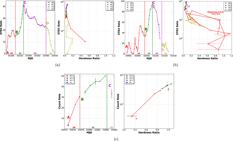
It is also informative to compare the hardness–intensity diagrams (HIDs) of LMC X-3 to these other sources. Generally transient X-ray binaries move in the so-called q-like shape as shown in Fender et al. (2004), where they begin dim and hard before brightening and then eventually softening before dimming and hardening again (moving in a counterclockwise manner). LMC X-3 HIDs show a variety of different behaviors in its long-term cycles. Using the PCA STD2 data from HEASARC, we calculated the hardness ratios (HRs) of several long-term cycles. The energy bands used were the 2–4 keV soft band and the hard band of 9–20 keV.
For the cycle occurring from MJD 55,172 to 55,449, the light curve and HID are shown in Figure 9. The different colors represent different time periods on the light curve, allowing us to see how the HR evolves over time. In this cycle, LMC X-3 does not follow a typical q-track. It is initially slightly hard before getting very soft and moves in a clockwise manner around the q-track. This clockwise behavior has been observed before in LMC X-3 by Cambier & Smith (2013). The overall shape is similar to the HIDs of persistent sources such as Cygnus X-1 as seen in Grinberg et al. (2013).
Figure 9. (a) The left panel shows LMC X-3's light curve of a typical cycle. It was created from PCA STD2 data over MJD 55,172–55,449 and is separated into four different epochs. The right panel shows the HID over the same cycle created from PCA STD2 data. The hardness ratio generally stays very soft and exhibits a slight clockwise track. (b) The left panel shows LMC X-3's light curve of a cycle immediately following ALS2. It was created from PCA STD2 data over MJD 54,940–55,172 and is separated into four different epochs. The right panel shows the HID over the same cycle created from PCA STD2 data. Typical normal transient q-like behavior is observed initially as it moves through the q-track counterclockwise before getting extremely soft. (c) The left panel shows LMC X-3's light curve of a cycle immediately following ALS3. It was created from XRT data over MJD 55,975–55,984 and is separated into three different epochs. The right panel shows the HID over the same cycle. LMC X-3 starts soft before getting harder at increasing count rates. Possible slight clockwise q-track behavior is observed.
Download figure:
Standard image High-resolution image
We calculated the HR for the cycle immediately following ALS2, and the HID and light curve are shown in Figure 9. This cycle was immediately prior to the previously discussed cycle and covers MJD 54,940 through 55,172. In this cycle, there is an indication of normal transient q-like behavior that occurs immediately upon exit of the ALS. It shows a general q-shape in a counterclockwise manner before getting extremely soft further into the cycle. This shape is reminiscent of the HID diagrams of GX 339-4, which can be found in Del Santo et al. (2009), though it is not as well defined.
We also studied the cycle following ALS3 with our XRT observations shown in Figure 9. The energy bands used were 0.3–1.5 keV for the soft band and 1.5–10 keV for the hard band. LMC X-3 starts soft before getting harder at increasing count rates. Possible slight clockwise q-track behavior is observed, though not similar to that of Cygnus X-1. It is clear, however, that the HIDs of normal cycles in LMC X-3 are different from HIDs of cycles just following an ALS. This implies that different processes occur within ALSs that are not observed in normal states.
Why is LMC X-3 different from a typical persistent or transient source? It may be because of its mass ratio. Orosz et al. (2011) found that the masses of Cygnus X-1's black hole and companion star are 14.8 ± 1.0  and 19.2 ± 1.9
  , respectively. This mass ratio of Cygnus X-1 is then 1.30 ± 0.16. For GX 339-4 the mass of its black hole is 7.5 ± 0.8 (Chen 2011), and for its companion star it is no greater than 1.1
  (Muñoz-Darias et al. 2008). The mass ratio of GX 339-4 is then much lower with an upper limit of 0.15 ± 0.02. LMC X-3 masses were found by Orosz et al. (2014) to be 6.95 ± 0.33
  for the black hole and 3.7 ± 0.24
  for the companion. The mass ratio falls in between Cygnus X-1 and GX 339-4 at 0.53 ± 0.04. This is also larger than the mass ratios of 16 transient X-ray binaries studied by Özel et al. (2010), with only two of them approaching LMC X-3's. The mass ratio could potentially play a role in LMC X-3's behavior in the HIDs, displaying characteristics of both persistent and transient X-ray binaries. We conclude that LMC X-3 is likely a transient source with a high duty cycle. This could explain why LMC X-3's luminosity relative to Eddington is more similar to the transient GX 339-4 and could explain the resemblance in HIDs to both GX 339-4 and Cygnus X-1 as well.
Our findings support the conclusions of Orosz et al. (2014), where they classify LMC X-3 as a transient black hole binary that is fed by Roche lobe overflow and has a possibly short recurrence time. In a study of simulations of potential progenitor systems (PPSs) of LMC X-3, Sørensen et al. (2016) found that ∼69% of the viable PPSs formed persistent binaries compared to only ∼31% of the PPSs forming transient binaries. While these simulations indicate a higher probability that LMC X-3 is a persistent binary, a transient binary is viable. The evidence from Orosz et al. (2014), coupled with our analysis, implies that LMC X-3 is likely a transient source that is usually in outburst.
5. Conclusions
The rich and diverse data set on LMC X-3 described here, including data from RXTE, Swift, XMM-Newton, and MAXI, has allowed us to undertake a thorough examination of the characteristics of the source during a normal low state compared to the ALS, from which we draw the following conclusions.
We determined that LMC X-3 began to enter its third ALS observed by RXTE. The PCA count rate fell below 2 counts s−1 PCU−1 on 2011 November 20 (MJD 55,885) and below 0.1 counts s−1 PCU−1 on 2011 December 2 (MJD 55,897), which we consider to be the start date of ALS3. The X-ray rate stayed at historically low values seen previously in ALS1, until the end of RXTE's mission in 2012 January. Continuous monitoring by MAXI and Swift shows ALS3 to continue for nearly 80 days until, on 2012 February 18 (MJD 55,975), a rapid flare was seen in XRT, signaling the end of ALS3 and the return of the more normal high-amplitude flux variability for the source. The low flux level and duration of ALS3 are similar to those of ALS1, which lasted 96 days (ALS2, which at ∼188 days lasted nearly twice as long as ALS1, did not reach these unprecedentedly low flux levels; Smale & Boyd 2012). From the beginning of ASM monitoring to 2016 June, the fraction of time LMC X-3 has spent in one of the three ALSs is 4.9%.
We also determined that while the entrances into ALS3 and a normal low state are very similar, the exits differ significantly. LMC X-3 exits ALS3 more than 12.8 times faster than it emerges from a typical low state, while also flaring to ∼2.5 times its typical flux, implying that the mechanism that drives the system out of the ALS is different from that which gives rise to the more typical flux variations.
We measure an ∼8-day lag in X-ray brightness compared to the UV, which is consistent with the 5- to 10-day lag found by Brocksopp et al. (2001) in optical/X-ray monitoring during normal variability, lending further evidence that a change in the mass accretion rate from the donor star appears to be driving the long-term variability, as well as the anomalous low states.
Aside from the X-ray lag, we find that the UV variability tracks the X-ray variability closely, consistent with the variability being caused by changes in the accretion flow from the companion. The UV flux during ALS3 is only ∼75% that of the UV flux during a normal low state, consistent with the disk component itself becoming a much less significant contributor to the overall UV flux during ALSs. This is also consistent with models predicting that the entire inner accretion disk evaporates for values of 0.001 LEDD and below (Liu et al. 2007; Taam et al. 2008).
During normal variability, the X-ray and UV flux of LMC X-3 is nearly always changing, either brightening or dimming as the source visits highs and lows in its ∼100-day timescale long-term variability. During this variability, the fraction of the UV light coming from the companion star varies significantly, ranging from ∼30%–40% in a typical state to ∼70%–80% in a normal low state. Spectral modeling shows that this variability is driven largely by changes in the accretion disk in the two-component model. In contrast, we find that ALS3, like ALS1, is remarkably flat with an unchanging and historically low X-ray flux, well fit by a pure hard power law, again consistent with an evaporated disk.
When exiting ALS2 and resuming its normal variability pattern, the source resembles the canonical transient GX 339-4, flaring dramatically and quickly, and tracing out a q-like diagram in hardness–intensity space for a short time. When exiting ALS3, the source traces a clockwise q-track, opposite its behavior following ALS2, but it is clear that the HIDs following these ALSs are different from the HIDs of normal cycles.
We conclude that ALSs in LMC X-3 are fundamentally different from its typical low states and may imply that this black hole binary is close to the persistent/transient source dividing line, making it a transient source that is "on" about 95% of the time.
This research has made use of Swift and RXTE data obtained from the High Energy Astrophysics Science Archive Research Center (HEASARC), provided by NASA's Goddard Space Flight Center. This research has also made use of the MAXI data provided by the RIKEN, JAXA, and MAXI teams. This work is also based on observations obtained with XMM-Newton, an ESA science mission with instruments and contributions directly funded by ESA Member States and the USA (NASA). This work made use of data supplied by the UK Swift Science Data Centre at the University of Leicester. T.T. acknowledges support of NASA grant NNX11AJ04G S06 to the Catholic University of America. We acknowledge the very helpful comments of Fred Bruhweiler, Jörn Wilms, and Joel Coley based on an earlier version of this manuscript, as well as the anonymous referee for their constructive feedback of this manuscript.
Facilities: HEASARC - , RXTE - , MAXI - , Swift - , XMM - .
Appendix: Swift Data
In Table 7 we present details of our Swift data, including the MJD, UV and X-ray flux, filter/mode information, and UV magnitudes. Low states are also identified.
Table 7. Swift Data: U, UVW1, UVW2, PC, WT
| MJD | Flux | Error | UV | Magnitude | UVOT | MJD | Flux | Error | X-ray XRT | State | Hardness | Error |
|---|---|---|---|---|---|---|---|---|---|---|---|---|
| (erg cm−2 s−1) | (erg cm−2 s−1) | Magnitude | Error | Filter | (mcrab) | (mcrab) | Mode | Ratio | ||||
| 55,871.03 | 1.88E−15 | 6.83E−17 | 17.87 | 0.04 | UVW2 | 55,871.50 | 20.68 | 0.10 | WT | 0.72 | 0.01 | |
| 55,897.03 | 1.85E−15 | 6.32E−17 | 17.89 | 0.04 | UVW2 | 55,897.04 | 0.09 | UL | WT | ALS3 | 0.57 | 0.60 |
| 55,927.72 | 1.84E−15 | 5.75E−17 | 17.89 | 0.03 | UVW2 | 55,927.72 | 0.06 | UL | WT | ALS3 | −0.23 | 0.41 |
| 55,930.13 | 1.47E−15 | 7.17E−17 | 18.13 | 0.05 | UVW2 | 55,930.16 | 0.05 | 0.03 | WT | ALS3 | 0.10 | 0.07 |
| 55,951.37 | 1.13E−15 | 4.22E−17 | 18.00 | 0.04 | UVW1 | 55,951.41 | 3.0E−4 | 0.0007 | PC | ALS3 | −0.48 | 0.67 |
| 55,953.31 | 1.81E−15 | 5.51E−17 | 17.91 | 0.03 | UVW2 | 55,953.38 | 0.24 | 0.19 | WT | ALS3 | 0.49 | 0.33 |
| 55,953.39 | 2.5E−3 | UL | PC | ALS3 | 1.06 | 0.17 | ||||||
| 55,955.20 | 1.32E−15 | 3.38E−17 | 17.83 | 0.03 | UVW1 | 55,955.20 | 6.1E−3 | UL | PC | ALS3 | 1.00 | 0.28 |
| 55,957.13 | 1.53E−15 | 3.67E−17 | 18.09 | 0.03 | UVW2 | 55,957.13 | 7.6E−3 | UL | PC | ALS3 | 0.68 | 0.17 |
| 55,959.07 | 9.72E−16 | 2.70E−17 | 18.16 | 0.03 | UVW1 | 55,959.08 | 7.8E−3 | UL | PC | ALS3 | 2.10 | 0.57 |
| 55,961.02 | 1.86E−15 | 8.21E−17 | 17.88 | 0.05 | UVW2 | 55,961.25 | 5.1E−3 | UL | PC | ALS3 | 0.65 | 0.19 |
| 55,963.21 | 9.63E−16 | 2.69E−17 | 18.17 | 0.03 | UVW1 | 55,963.22 | 7.2E−3 | UL | PC | ALS3 | 0.52 | 0.16 |
| 55,967.01 | 1.29E−15 | 3.48E−17 | 17.86 | 0.03 | UVW1 | 55,967.02 | 8.9E−3 | UL | PC | ALS3 | 0.89 | 0.25 |
| 55,975.53 | 1.72E−15 | 6.62E−17 | 17.54 | 0.04 | UVW1 | 55,975.66 | 5.42 | 0.63 | WT | ALS3 | 0.34 | 0.09 |
| 55,975.67 | 5.61 | 0.18 | PC | ALS3 | 0.42 | 0.03 | ||||||
| 55,976.93 | 33.86 | 0.21 | WT | ALS3 | 0.75 | 0.01 | ||||||
| 55,977.73 | 2.94E−15 | 5.76E−17 | 17.38 | 0.02 | UVW2 | 55,977.74 | 43.55 | 0.26 | WT | ⋯ | 0.86 | 0.01 |
| 55,978.74 | 43.64 | 0.28 | WT | ⋯ | 0.89 | 0.01 | ||||||
| 55,979.67 | 2.17E−15 | 4.93E−17 | 17.29 | 0.02 | UVW1 | 55,979.68 | 57.91 | 0.32 | WT | ⋯ | 0.96 | 0.01 |
| 55,980.60 | 1.40E−15 | 2.80E−17 | 17.05 | 0.02 | U | 55,980.61 | 63.40 | 0.36 | WT | ⋯ | 0.98 | 0.01 |
| 55,981.41 | 3.16E−15 | 8.93E−17 | 17.30 | 0.03 | UVW2 | 55,981.42 | 64.03 | 0.55 | WT | ⋯ | 0.98 | 0.02 |
| 55,982.42 | 71.45 | 0.62 | WT | ⋯ | 1.06 | 0.02 | ||||||
| 55,983.55 | 1.85E−15 | 4.41E−17 | 17.46 | 0.03 | UVW1 | 55,983.55 | 54.77 | 0.41 | WT | ⋯ | 1.00 | 0.01 |
| 56,055.78 | 3.46E−15 | 7.04E−17 | 16.78 | 0.02 | UVW1 | 56,055.79 | 55.97 | 0.33 | WT | ⋯ | 1.05 | 0.01 |
| 56,089.01 | 5.10E−15 | 1.03E−16 | 16.79 | 0.02 | UVW2 | 56,089.02 | 61.98 | 0.43 | WT | ⋯ | 1.08 | 0.01 |
| 56,112.99 | 3.91E−15 | 8.40E−17 | 17.07 | 0.02 | UVW2 | 56,113.00 | 54.52 | 3.28 | PC | ⋯ | 1.38 | 0.17 |
| 56,113.01 | 60.86 | 0.54 | WT | 1.04 | 0.02 | |||||||
| 56,141.73 | 4.25E−15 | 6.99E−17 | 16.99 | 0.02 | UVW2 | 56,141.61 | 52.21 | 0.27 | WT | ⋯ | 1.05 | 0.01 |
| 56,145.04 | 3.77E−15 | 5.49E−17 | 17.11 | 0.02 | UVW2 | 56,145.05 | 50.54 | 0.17 | WT | ⋯ | 1.02 | 0.01 |
| 56,163.81 | 3.24E−15 | 4.63E−17 | 17.28 | 0.02 | UVW2 | 56,163.82 | 48.69 | 0.14 | WT | ⋯ | 0.96 | 0.01 |
| 56,165.98 | 2.99E−15 | 6.18E−17 | 17.37 | 0.02 | UVW2 | 56,165.99 | 47.17 | 0.30 | WT | ⋯ | 0.99 | 0.01 |
| 56,168.62 | 3.00E−15 | 4.73E−17 | 17.36 | 0.02 | UVW2 | 56,168.63 | 46.81 | 0.20 | WT | ⋯ | 0.92 | 0.01 |
| 56,175.43 | 2.76E−15 | 5.83E−17 | 17.45 | 0.02 | UVW2 | 56,175.44 | 46.21 | 0.31 | WT | ⋯ | 0.92 | 0.01 |
| 56,333.20 | 2.85E−15 | 4.81E−17 | 17.42 | 0.02 | UVW2 | 56,333.22 | 48.60 | 0.19 | WT | ⋯ | 0.90 | 0.01 |
| 56,345.61 | 2.75E−15 | 4.58E−17 | 17.46 | 0.02 | UVW2 | 56,345.62 | 46.94 | 0.23 | WT | ⋯ | 0.86 | 0.01 |
| 56,353.22 | 2.72E−15 | 4.87E−17 | 17.47 | 0.02 | UVW2 | 56,353.23 | 36.91 | 0.21 | WT | NL | 0.76 | 0.01 |
| 56,361.12 | 2.44E−15 | 6.10E−17 | 17.59 | 0.03 | UVW2 | 56,361.13 | 24.54 | 0.25 | WT | NL | 0.65 | 0.01 |
| 56,364.19 | 2.35E−15 | 4.53E−17 | 17.63 | 0.02 | UVW2 | 56,364.21 | 18.27 | 0.14 | WT | NL | 0.62 | 0.01 |
| 56,365.71 | 2.01E−15 | 6.04E−17 | 17.80 | 0.03 | UVW2 | 56,365.72 | 17.67 | 0.64 | PC | NL | 0.68 | 0.05 |
| 56,367.22 | 1.36E−15 | 4.73E−17 | 17.80 | 0.04 | UVW1 | 56,367.24 | 15.12 | 0.22 | WT | NL | 0.56 | 0.02 |
| 56,368.29 | 1.00E−15 | 3.14E−17 | 17.41 | 0.03 | U | 56,368.30 | 15.01 | 0.22 | WT | NL | 0.54 | 0.02 |
| 56,369.34 | 2.30E−15 | 3.98E−17 | 17.65 | 0.02 | UVW2 | 56,369.35 | 12.96 | 0.10 | WT | NL | 0.51 | 0.01 |
| 56,370.06 | 12.65 | 0.19 | WT | NL | 0.53 | 0.02 | ||||||
| 56,371.64 | 1.57E−15 | 4.70E−17 | 17.64 | 0.03 | UVW1 | 56,371.66 | 10.64 | 0.17 | WT | NL | 0.46 | 0.02 |
| 56,372.23 | 9.25E−16 | 2.93E−17 | 17.50 | 0.03 | U | 56,372.24 | 10.04 | 0.21 | WT | NL | 0.50 | 0.02 |
| 56,372.25 | 12.68 | 0.87 | PC | NL | 0.57 | 0.08 | ||||||
| 56,373.44 | 2.29E−15 | 6.51E−17 | 17.66 | 0.03 | UVW2 | 56,373.45 | 11.51 | 0.73 | PC | NL | 0.59 | 0.08 |
| 56,373.45 | 8.67 | 0.22 | WT | NL | 0.45 | 0.02 | ||||||
| 56,377.41 | 1.86E−15 | 3.53E−17 | 17.88 | 0.02 | UVW2 | 56,377.42 | 6.90 | 0.08 | WT | NL | 0.38 | 0.01 |
| 56,379.65 | 1.78E−15 | 5.01E−17 | 17.51 | 0.03 | UVW1 | 56,379.66 | 5.80 | 0.69 | WT | NL | 0.60 | 0.14 |
| 56,379.67 | 8.22 | 0.32 | PC | NL | 0.52 | 0.04 | ||||||
| 56,380.25 | 9.58E−16 | 2.93E−17 | 17.45 | 0.03 | U | 56,380.26 | 7.71 | 0.32 | PC | NL | 0.50 | 0.05 |
| 56,380.26 | 6.52 | 0.43 | WT | NL | 0.39 | 0.05 | ||||||
| 56,381.59 | 2.26E−15 | 5.98E−17 | 17.67 | 0.03 | UVW2 | 56,381.61 | 6.43 | 0.24 | PC | NL | 0.44 | 0.04 |
| 56,382.07 | 6.82 | 0.28 | PC | NL | 0.54 | 0.05 | ||||||
| 56,382.07 | 6.33 | 0.82 | WT | NL | 0.52 | 0.13 | ||||||
| 56,382.99 | 1.86E−15 | 5.36E−17 | 17.46 | 0.03 | UVW1 | 56,383.01 | 6.74 | 0.69 | WT | NL | 0.35 | 0.08 |
| 56,383.01 | 7.51 | 0.37 | PC | NL | 0.51 | 0.05 | ||||||
| 56,384.13 | 1.02E−15 | 3.02E−17 | 17.39 | 0.03 | U | 56,384.14 | 10.48 | 0.43 | PC | NL | 0.58 | 0.05 |
| 56,385.12 | 2.16E−15 | 3.90E−17 | 17.72 | 0.02 | UVW2 | 56,385.14 | 10.83 | 0.09 | WT | NL | 0.54 | 0.01 |
| 56,392.75 | 1.18E−15 | 2.57E−17 | 17.23 | 0.02 | U | 56,392.76 | 24.85 | 0.20 | WT | NL | 0.70 | 0.01 |
| 56,393.72 | 2.47E−15 | 5.53E−17 | 17.57 | 0.02 | UVW2 | 56,393.73 | 26.02 | 0.22 | WT | NL | 0.71 | 0.01 |
| 56,394.70 | 26.71 | 0.20 | WT | NL | 0.75 | 0.01 | ||||||
| 56,395.82 | 2.14E−15 | 5.03E−17 | 17.30 | 0.03 | UVW1 | 56,395.84 | 21.04 | 0.26 | WT | ⋯ | 0.72 | 0.02 |
| 56,396.62 | 1.39E−15 | 3.09E−17 | 17.05 | 0.02 | U | 56,396.63 | 25.17 | 0.27 | WT | ⋯ | 0.71 | 0.02 |
| 56,397.55 | 3.02E−15 | 8.73E−17 | 17.35 | 0.03 | UVW2 | 56,397.57 | 31.51 | 0.57 | WT | ⋯ | 0.79 | 0.03 |
| 56,398.30 | 29.60 | 0.27 | WT | ⋯ | 0.78 | 0.01 |
Note. Entries without errors denote observations resulting only in an upper limit estimate, and the error is marked as UL. Only low states are identified.
Footnotes
- 4
- 5
- 6
- 7
- 8
- 9
- 10
- 11