


ABSTRACT
Since the peculiar nature of Lambda Boötis was first noticed in 1943, the Lambda Boo stars have been recognized as a group of peculiar A-type stars. They are Population I dwarfs that show deficiencies of iron-peak elements (up to 2 dex), but have near-solar C, N, O, and S abundances. In a previous paper, we used both observed and synthetic ultraviolet spectra to demonstrate that the C i 1657 Å/Al ii 1671 Å equivalent width ratio can help distinguish between Lambda Boo stars and other metal-weak stars hotter than 8000 K. In this paper, using observed and synthetic visible (4000–6800 Å) spectra, we demonstrate that the C i 5052.17 Å/Mg ii 4481 Å equivalent width ratio can be used as a quantitative diagnostic for cooler Lambda Boo stars.
Export citation and abstract BibTeX RIS
1. INTRODUCTION
The Lambda Boo class is a subgroup of late B- to early F-type stars that have an unusually low abundance of iron-peak elements in their surface layers. The prototype, Lambda Boötis (HD 125162; A3VakB9mB9 lambda Boo; see Gray et al. 2003), was first reported as peculiar by Morgan et al. (1943). Over the past 70+ years, more than 200 Lambda Boo candidates published in the literature have been selected using different criteria. The distinguishing characteristic in a Lambda Boo star's spectrum is the overall weakness of metallic lines, but their C, N, O, and S abundances are near solar. A good portion of these Lambda Boo candidates have been identified by visually examining the difference between their low-resolution spectra and spectra of standard stars. However, some ambiguity remains, especially for mild or borderline Lambda Boo stars.
Murphy et al. (2015) carried out a systematic review of published papers for all previously identified Lambda Boo candidates. Cheng et al. 2016 (hereafter Paper I) utilized synthetic ultraviolet spectra to explore the physical basis for the classification of Lambda Boo stars, demonstrating that the C i 1657 Å/Al ii 1671 Å equivalent width ratio is the best quantitative UV criterion to distinguish between Lambda Boo stars and other metal-weak stars hotter than 8000 K. Since cooler Lambda Boo stars (late A type and early F type) do not have enough flux shortward of 1700 Å, we sought similar diagnostic ratios in the visible wavelength range.
Lambda Boo-type stars are not overall metal-weak, because their C, N, O, and S abundances tend to be near solar. Since we seek to understand the cause of this distinctive abundance pattern, the diagnostic line ratios we are looking for should be based on the relative strength of light (e.g., C, O) and heavier elements (e.g., Mg, Al). We obtained high-resolution visible spectra for our program Lambda Boo stars, normal/reference stars, and non-Lambda Boo stars from the ELODIE and ESO archives.6
 7
7
In this paper, our specific goals are to:
- 1.establish a "quantitative" classification criterion using visible spectra that helps distinguish Lambda Boo stars from normal stars and other metal-weak stars with Teff < 8000 K (see Section 4 for details), and
- 2.demonstrate how synthetic spectra (models) can be used to study the characteristics of Lambda Boo stars.
2. PROGRAM STARS
2.1. Confirmed Lambda Boo Stars
As discussed in Paper I, Lambda Boo candidates have been selected using several different criteria, and sometimes the agreement among the published lists is quite poor. A common set of Lambda Boo-class characteristics is required to discriminate between theories explaining the origin of the Lambda Boo phenomenon. We started with a list of over 200 stars cited in the literature as Lambda Boo stars. This list led to the compilation of possible Lambda Boo stars presented in Murphy et al. (2015). In this paper we carry out a more detailed evaluation of the visible properties of the 64 "confirmed" Lambda Boo stars listed in Murphy et al. (2015). These "confirmed" members are not concentrated in any particular region in the sky (see Figure 1). Among them, 47 Lambda Boo stars have high-resolution archival visible spectra. Because we are exploring quantifiable classification criteria for the Lambda Boo class as a function of Teff and [M/H], we searched for all of the published Teff and [M/H] values for each program star in our study. We assigned a "mean" effective temperature to each star based on a range of temperatures found in the literature (excluding any outliers), and we did not include any duplicate temperatures. We also limited the number of sources included in this range to the five values that best represent the data set for each star. The mean effective temperature, a range of effective temperatures, and the observations (data sets) we used in this paper are listed in Table 1. We also list previously published metallicity values, which allow us to compare our program stars to models with different metallicities. The methods that have been used to determine metallicity differ from paper to paper, and sometimes [M/H] and [Fe/H] are used interchangeably. We cite them as [M/H] or [Fe/H] based on how they are labeled in their original publications. Of our 64 program Lambda Boo stars, 62 have literature log g values. The average log g value for those 62 program Lambda Boo stars is 4.01 (Figure 2(a)). Of our 64 program Lambda Boo-type stars, 48 have literature v sin i values. Because the median v sin i value of those 48 confirmed Lambda Boo stars with literature values is about 100 km s−1 (Figure 2(b)), we explored how rotational broadening affects our equivalent width measurement (see Sections 4.4 and 5).

Figure 1. Distribution of our 64 program Lambda Boo stars in the sky (in celestial coordinates). Note that there is no concentration in any specific region. The unfilled circles are those program Lambda Boo stars without archival visible spectra.
Download figure:
Standard image High-resolution image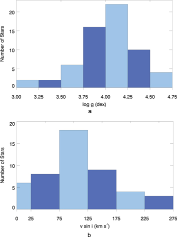
Figure 2. (a) Histogram of the log g distribution for 62 of our 64 program Lambda Boo stars that have literature log g values. The average log g for these 62 program Lambda Boo stars is 4.01. (b) Histogram of the projected rotational velocity distributions for 48 of our 64 program Lambda Boo stars that have literature v sin i values. The average v sin i for this sample is about 100 km s−1.
Download figure:
Standard image High-resolution imageTable 1. Lambda Boo Stars
| Identificationa | Mean Teff | Teff Differenceb | [Fe/H] | [M/H] | v sin ic | Data Set | S/Nd |
|---|---|---|---|---|---|---|---|
| (K) | (K) | bin | |||||
| HD 141569 | 10260 (2), (3), (4), (5) | −260/+240 | −0.5 (47) | ... | f | ELODIE 19970703/0014 | 158 |
| HD 294253 | 10103 (1), (9) | −798/+798 | −0.54 (1) | ... | b | FEROS 2009-12-02T07:52:58.138 | 164 |
| HD 170680 | 9774 (7), (8), (9) | −151/+226 | −0.4 (7) | ... | f | FEROS 2009-06-05T04:42:29.580 | 313 |
| HD 23392 | 9759 (2), (9), (10) | −494/+741 | ... | ... | d | FEROS 2010-07-22T09:18:51.642 | 208 |
| HD 36726 | 9542 (1), (9), (11), (27) | −222/+258 | −0.58 (1) | ... | c | FEROS 2009-12-04T06:34:07.441 | 231 |
| HD 130767 | 9209 (9), (11), (12) | −14/+18 | ... | ... | d | ELODIE 20020331/0010 | 140 |
| HD 37411 | 9100 (13) | −0/+0 | ... | −1.5 (48) | e | FEROS 2010-01-28T04:11:12.612 | 107 |
| HD 183324 | 9050 (8), (12), (14), (15) | −350/+250 | −1.24 (54) | −1.80 (49) | c | FEROS 2010-07-22T05:02:20.981 | 352 |
| HD 110411 | 8976 (7), (11), (16), (17) | −176/+224 | −1.0 (7) | −1.10 (40) | d | ELODIE 20040519/0017 | 209 |
| HD 31295 | 8871 (8), (12), (15), (16), (18) | −96/+119 | −0.89 (15) | −1.24 (40) | c | ELODIE 20031105/0069 | 225 |
| HD 74873 | 8815 (12), (19), (20), (21) | −225/+435 | −0.01 (50) | ... | c | HARPS 2014-09-16T11:04:01.560 | 193 |
| HD 221756 | 8733 (8), (12), (16), (17), (18) | −223/+287 | −0.64 (18) | −0.75 (49) | c | ELODIE 20011127/0012 | 107 |
| HD 125162 | 8700 (12), (17), (22), (23) | −50/+29 | −2.05 (22) | −2.00 (49) | c | ELODIE 19960522/0014 | 303 |
| HD 101412 | 8500 (6), (59), (60) | −200/+300 | −1.0 (4) | ... | a | HARPS 2014-09-23T11:03:07.090 | 80 |
| HD 120500 | 8394 (1), (9) | −7/+7 | −0.67 (51) | ... | d | FEROS 2009-06-06T00:49:43.346 | 357 |
| HD 319 | 8348 (12), (14), (15), (18) | −328/+294 | −0.35 (18) | ... | b | HARPS 2014-10-02T10:00:01.553 | 213 |
| HD 35242 | 8327 (9), (10), (12), (27) | −190/+184 | ... | ... | c | ELODIE 20030122/0007 | 168 |
| HD 153747 | 8256 (11), (12), (28) | −52/+104 | 0.00 (50) | ... | c | HARPS 2014-09-26T16:53:39.050 | 134 |
| HD 204041 | 8239 (14), (15), (29) | −239/+378 | −0.44 (18) | −0.83 (19) | b | FEROS 2009-06-05T06:59:05.057 | 229 |
| HD 91130 | 8159 (1), (9), (10), (11), (30) | −159/+199 | −1.69 (1) | ... | d | ELODIE 19970322/0015 | 124 |
| HD 105759 | 8157 (2), (9) | −443/+443 | ... | ... | c | FEROS 2009-06-04T02:41:19.045 | 382 |
| HD 192640 | 7988 (11), (15), (31) | −45/+42 | −2.0 (31) | ... | c | ELODIE 19990604/0032 | 324 |
| HD 30422 | 7977 (9), (10), (11), (32) | −107/+210 | −0.02 (50) | −0.52 (19) | c | FEROS 2009-12-05T06:35:55.983 | 371 |
| HD 11413 | 7956 (5), (9), (16), (33) | −31/+42 | −1.5 (16) | −2.03 (52) | d | FEROS 2010-07-22T10:39:57.651 | 366 |
| HD 198160 | 7912 (10), (16), (34), (35) | −316/+169 | −0.850 (16) | −1.00 (34) | e | FEROS 2010-08-31T01:06:00.125 | 261 |
| HD 290799 | 7864 (5), (9), (12), (36) | −151/+136 | −0.97 (1) | ... | b | FEROS 2009-12-05T07:17:58.019 | 97 |
| HD 111604 | 7798 (1), (9), (17) | −198/+202 | −1.08 (1) | −0.75 (49) | e | ELODIE 19960502/0029 | 157 |
| HD 193256 | 7739 (9), (10), (16) | −653/+531 | −0.95 (63) | ... | f | FEROS 2009-06-09T10:14:21.058 | 243 |
| HD 168740 | 7582 (9), (10), (37) | −182/+292 | ... | 0.0 (43) | d | FEROS 2009-06-02T07:05:57.888 | 453 |
| HD 210111 | 7521 (5), (9), (10), (16), (23) | −71/+72 | −1.1 (16) | −1.0 (53) | b | FEROS 2009-11-29T02:01:05.469 | 359 |
| HD 111786 | 7500 (8), (14), (15) | −50/+49 | −1.45 (54) | −0.58 (55) | d | FEROS 2009-06-07T23:34:24.541 | 160 |
| HD 139614 | 7500 (4), (38) | −100/+100 | −0.5 (4) | ... | a | FEROS 2009-06-10T03:49:51.778 | 226 |
| HD 218396 | 7465 (9), (27), (39), (40) | −110/+121 | −0.7 (62) | −0.47 (25) | b | ELODIE 20030730/0010 | 336 |
| HD 87271 | 7434 (9), (10), (11) | −233/+151 | ... | ... | c | ELODIE 20030121/0011 | 104 |
| HD 174005 | 7412 (9), (10), (41) | −292/+325 | −0.20 (56) | −0.77 (61) | c | FEROS 2009-06-03T07:28:27.034 | 333 |
| HD 75654 | 7341 (9), (10), (11), (19) | −81/+90 | −0.02 (50) | −0.95 (19) | b | FEROS 2010-01-27T06:04:24.542 | 386 |
| HD 7908 | 7340 (2), (9), (34), (42) | −337/+510 | −0.03 (50) | ... | c | FEROS 2010-01-29T01:15:24.839 | 291 |
| HD 6870 | 7337 (9), (11), (19) | −97/+107 | ... | −1.08 (19) | d | FEROS 2009-12-05T00:54:59.865 | 235 |
| HD 107233 | 7274 (9), (10), (32) | −74/+96 | ... | ... | c | FEROS 2010-03-08T06:07:26.136 | 283 |
| HD 142703 | 7231 (8), (11), (14), (15), (43) | −31/+30 | −1.10 (18) | ... | c | FEROS 2010-03-05T09:36:21.595 | 360 |
| HD 120896 | 7213 (9), (10), (37) | −194/+171 | −0.074 (57) | −0.5 (58) | c | FEROS 2009-06-06T00:59:59.932 | 266 |
| HD 13755 | 7195 (2), (9), (10), (42) | −119/+105 | 0.15 (34) | −0.18 (34) | c | FEROS 2009-12-08T03:07:21.235 | 121 |
| HD 15165 | 7157 (11), (44) | −143/+143 | −0.46 (44) | ... | c | ELODIE 20020813/0028 | 246 |
| HD 64491 | 7055 (5), (9), (30), (45), (46) | −147/+104 | ... | ... | a | ELODIE 20020328/0022 | 138 |
| HD 142994 | 7016 (9), (29) | −66/+66 | −0.56 (29) | −0.88 (19) | e | HARPS 2014-09-26T16:52:50.327 | 176 |
| HD 106223 | 6769 (1), (7), (9), (37) | −269/+231 | −1.44 (7) | ... | c | ELODIE 20030121/0012 | 135 |
| HD 4158 | 6483 (19), (30), (32) | −83/+67 | −0.17 (9) | −1.59 (19) | c | FEROS 2009-12-14T00:48:21.918 | 135 |
Notes.
aNote that these stars are listed in descending Teff order to assist with locating each star in Figure 10. bThe difference between the mean effective temperature and the lowest/highest effective temperature. cThe v sin i bin indicates the wavelength ranges listed in Table 4 that we used to measure this star's equivalent width values. Each star's v sin i bin was determined by comparing their observed spectra to models with similar stellar parameters. dSignal-to-noise ratios are provided for ELODIE, HARPS, and X-SHOOTER data by the ELODIE and ESO archives, respectively. We estimated signal-to-noise ratios for the FEROS data near 5500 Å.References. (1) Andrievsky et al. (2002), (2) Wright et al. (2003), (3) Wyatt et al. (2007), (4) Guimarães et al. (2006), (5) Soubiran et al. (2010), (6) Cowley et al. (2010), (7) Heiter (2002), (8) Solano & Paunzen (1999), (9) Ammons et al. (2006), (10) McDonald et al. (2012), (11) Paunzen et al. (2002a), (12) Paunzen et al. (2002b), (13) Maaskant et al. (2014), (14) Koleva & Vazdekis (2012), (15) Cenarro et al. (2007), (16) Sturenburg (1993), (17) Hauck et al. (1998), (18) Prugniel et al. (2011), (19) Gerbaldi et al. (2003), (20) Paunzen et al. (1998), (21) Mittal et al. (2015), (22) Venn & Lambert (1990), (23) Paunzen et al. (2003), (24) Koleva & Vazdekis (2012), (25) Gray & Kaye (1999), (26) Zorec & Royer (2012), (27) Allende Prieto & Lambert (1999), (28) Xu et al. (2002), (29) Solano et al. (2001), (30) Kamp et al. (2001), (31) Heiter et al. (1998), (32) Solano & Paunzen (1998), (33) Koen et al. (2003), (34) Kordopatis et al. (2013), (35) David & Hillenbrand (2015), (36) Faraggiana et al. (1997), (37) Masana et al. (2006), (38) Labadie et al. (2014), (39) Cuypers et al. (2009), (40) Gray et al. (2003), (41) Ammler-von Eiff & Reiners (2012), (42) Lafrasse et al. (2010), (43) North et al. (1994), (44) Andrievsky et al. (1995), (45) Muñoz Bermejo et al. (2013), (46) Kamp et al. (2002), (47) Merín et al. (2004), (48) Gray & Corbally (1998), (49) Griffin et al. (2012), (50) Gontcharov (2012), (51) Anderson & Francis (2012), (52) Faraggiana et al. (2004), (53) Paunzen et al. (2012), (54) Saffe et al. (2008), (55) Ohanesyan (2008), (56) Marsakov & Shevelev (1995), (57) Luo et al. (2015), (58) Paunzen (2015), (59) Folsom et al. (2012), (60) Hubrig et al. (2010), (61) Faraggiana et al. (2001), (62) Gebran et al. (2016), (63) Paunzen et al. (2001).
Download table as: ASCIITypeset image
2.2. Normal Reference Stars
We compared our Lambda Boo stars with a set of normal (standard) stars selected from the literature. This includes various sources of MK standards (Mamajek's website,8 the "IUE Ultraviolet Spectral Atlas of Standard Stars,"9 Royer et al. 2014, and Jaschek & Gomez 1998). The normal stars used in this study can be found in Table 2. Not all of the "normal" reference stars have solar abundances and [M/H] = 0. As shown in Table 2, their previously published [M/H] values range from +0.15 to −0.49 dex.
Table 2. Normal (Standard) Stars
| Identificationa | Mean Teff | Teff Differenceb | [Fe/H] | [M/H] | v sin ic | Data Set | S/Nd |
|---|---|---|---|---|---|---|---|
| (K) | (K) | bin | |||||
| HD 196867 | 11012 (1), (2), (3) | −307/+208 | −0.06 (45) | −0.49 (46) | d | ELODIE 20031005/0014 | 196 |
| HD 85504 | 10041 (4), (5), (6), (7), (8) | −280/+159 | −0.14 (45) | 0.0 (47) | b | ELODIE 19960424/0026 | 120 |
| HD 133962 | 9890 (4), (7), (8), (9), (10) | −660/+610 | 0.019 (7) | ... | b | ELODIE 20050421/0047 | 210 |
| HD 71155 | 9755 (11), (12), (13) | −199/+195 | −0.40 (48) | −0.44 (11) | d | ELODIE 20040328/0028 | 329 |
| HD 89774 | 9717 (4), (7), (8), (9), (10) | −487/+983 | −0.038 (7) | ... | b | ELODIE 20050422/0015 | 101 |
| HD 58142 | 9599 (4), (7), (8), (9), (10) | −137/+401 | −0.004 (7) | −0.24 (46) | a | ELODIE 20050203/0012 | 437 |
| HD 132145 | 9568 (4), (7), (8), (9), (14) | −284/+432 | −0.097 (7) | ... | a | ELODIE 20050421/0045 | 185 |
| HD 104181 | 9564 (4), (7), (8), (10), (14) | −64/+96 | −0.207 (7) | ... | b | ELODIE 20040426/0037 | 230 |
| HD 145788 | 9555 (4), (7), (10), (14), (15) | −145/+195 | −0.137 (7) | −0.22 (57) | a | ELODIE 20060601/0015 | 96 |
| HD 103287 | 9379 (1), (11), (16) | −107/+124 | −0.44 (1) | −0.19 (11) | e | ELODIE 19961230/0019 | 277 |
| HD 23948 | 9088 (8), (10), (17), (18) | −118/+149 | −0.130 (17) | −0.47 (57) | c | ELODIE 20040106/0010 | 160 |
| HD 102647 | 8632 (12), (11), (21) | −254/+225 | −0.40 (12) | 0.00 (11) | d | ELODIE 20040229/0047 | 305 |
| HD 87696 | 8044 (4), (8), (10), (18), (22) | −194/+206 | ... | 0.15 (49) | d | ELODIE 19970221/0030 | 289 |
| HD 158352 | 7648 (4), (8), (10), (18), (23) | −218/+205 | −0.06 (45) | ... | e | ELODIE 19950606/0008 | 284 |
| HD 187642 | 7623 (4), (24), (25), (26) | −73/+104 | −0.24 (45) | 0.02 (11) | f | ELODIE 20031001/0016 | 280 |
| HD 211336 | 7511 (8), (18), (27), (28) | −171/+279 | 0.08 (45) | 0.04 (50) | c | ELODIE 19970919/0014 | 430 |
| HD 91480 | 6977 (11), (29), (30), (31), (32) | −79/+37 | −0.12 (51) | −0.05 (11) | b | ELODIE 20050203/0014 | 483 |
| HD 58946 | 6955 (1), (4), (12), (30), (33) | −56/+43 | −0.25 (45) | −0.21 (11) | b | ELODIE 20040202/0044 | 267 |
| HD 113139 | 6893 (11), (18), (31), (32), (34) | −64/+27 | 0.02 (52) | −0.10 (11) | c | ELODIE 20040513/0011 | 540 |
| HD 134083 | 6571 (11), (12), (35) | −31/+29 | 0.10 (53) | −0.08 (11) | b | ELODIE 19990602/0020 | 348 |
| HD 30652 | 6512 (29), (33), (36), (37), (38) | −35/+26 | 0.00 (37) | −0.17 (36) | a | ELODIE 20040229/0020 | 253 |
| HD 222368 | 6392 (8), (29), (33), (39) | −104/+130 | −0.12 (37) | −0.10 (34) | a | ELODIE 19971017/0013 | 360 |
| HD 142860 | 6371 (29), (37), (38), (39), (40) | −58/+125 | −0.18 (54) | −0.20 (55) | a | ELODIE 20040229/0064 | 298 |
| HD 16895 | 6324 (29), (31), (37), (41), (42) | −15/+18 | −0.02 (37) | −0.13 (40) | a | ELODIE 20030929/0039 | 295 |
| HD 126660 | 6278 (35), (43), (44) | −76/+60 | 0.02 (35) | −0.01 (56) | b | ELODIE 19990601/0010 | 333 |
Notes.
aNote that these stars are listed in descending Teff order to assist with locating each star in Figure 10. bThe difference between the mean effective temperature and the lowest/highest effective temperature. cThe v sin i bin indicates the wavelength ranges listed in Table 4 that we used to measure this star's equivalent width values. Each star's v sin i bin was determined by comparing their observed spectra to models with similar stellar parameters. dSignal-to-noise ratios are provided by the ELODIE archive.References. (1) Wu et al. (2011), (2) Sokolov (1995), (3) Zorec et al. (2009), (4) Zorec & Royer (2012), (5) Adelman & Philip (1992), (6) Adelman & Philip (1994), (7) Royer et al. (2014), (8) Ammons et al. (2006), (9) Gebran et al. (2016), (10) Wright et al. (2003), (11) Gray et al. (2003), (12) Solano & Paunzen (1999), (13) Katz et al. (2011), (14) Lafrasse et al. (2010), (15) Fossati et al. (2009), (16) McDonald et al. (2012), (17) Gebran & Monier (2008), (18) David & Hillenbrand (2015), (19) Hill (1995), (20) Kontizas & Theodossiou (1980), (21) Malagnini & Morossi (1997), (22) Chen et al. (2014), (23) Masana et al. (2006), (24) Erspamer & North (2003), (25) di Benedetto (1998), (26) Allende Prieto et al. (2004), (27) Gerbaldi et al. (2007), (28) Önehag et al. (2009), (29) Marsakov & Shevelev (1995), (30) Casagrande et al. (2011), (31) Suchkov et al. (2003), (32) Ammler-von Eiff & Reiners (2012), (33) Boyajian et al. (2012), (34) Gray et al. (2001), (35) Prugniel et al. (2011), (36) Franchini et al. (2014), (37) Ramírez et al. (2013), (38) Moro-Martín et al. (2015), (39) van Belle & von Braun (2009), (40) Edvardsson et al. (1993), (41) Ramírez et al. (2012), (42) Valdes et al. (2004), (43) Balachandran (1990), (44) Cenarro et al. (2007), (45) Anderson & Francis (2012), (46) Fitzpatrick & Massa (2005), (47) Cacciari et al. (1987), (48) Prugniel et al. (2007), (49) Griffin et al. (2012), (50) North et al. (1997), (51) Pace (2013), (52) Cesetti et al. (2013), (53) Blackwell & Lynas-Gray (1994), (54) Lawler et al. (2009), (55) López-Valdivia et al. (2014), (56) Mann et al. (2013), (57) Kordopatis et al. (2013).
Download table as: ASCIITypeset image
2.3. Non-Lambda Boo Stars Used to Test Our Visible Classification Criterion
Murphy et al. (2015) re-evaluated 212 objects that have been considered as Lambda Boo candidates based on their literature searches. Their membership recommendation was then made into one of four classes: member, probable member, uncertain member, or nonmember. Of their 103 nonmembers, 43 have existing high-resolution archival visible spectra (see Section 3 and Table 3). In this paper, we have tested our new visible Lambda Boo classification criterion on these nonmembers (see details in Section 5).
Table 3. Nonmember Stars
| Identificationa | Mean Teff | Teff Differenceb | [Fe/H] | [M/H] | v sin ic | Data Set | S/Nd |
|---|---|---|---|---|---|---|---|
| (K) | (K) | bin | |||||
| HD 78316 | 12643 (5), (6), (22), (29), (56) | −743/+806 | 0.12 (29) | ... | a | FEROS 2012-01-07T07:02:20.361 | 256 |
| HD 37886 | 12050 (6), (46), (57) | −850/+500 | ... | ... | a | FEROS 2009-12-07T05:43:37.558 | 146 |
| HD 22470 | 11990 (6), (8), (13), (58) | −1331/+1042 | 0.00 (40) | ... | c | FEROS 2011-01-22T03:03:23.323 | 270 |
| HD 177756 | 11249 (1), (2), (3), (4), (5) | −749/+713 | −0.08 (5) | −0.50 (18) | e | ELODIE 20001004/0019 | 302 |
| HD 130158 | 10719 (1), (2), (6), (46), (47) | −257/+281 | 0.00 (40) | ... | b | FEROS 2006-06-29T00:03:38.146 | 422 |
| HD 169009 | 10627 (2), (6), (18), (46), (48) | −370/+373 | −0.01 (40) | 0.00 (18) | b | FEROS 2009-06-03T07:06:37.204 | 284 |
| HD 79469 | 10392 (1), (2), (6), (7), (8) | −602/+808 | 0.4 (36) | ... | c | ELODIE 19970122/0011 | 371 |
| HD 212061 | 10382 (1), (2), (3), (7), (9) | −592/+268 | −0.35 (7) | ... | c | ELODIE 20011128/0009 | 162 |
| HD 123299 | 10250 (3), (4), (37) | −150/+180 | −0.56 (37) | ... | a | ELODIE 20030115/0048 | 417 |
| HD 153808 | 9898 (2), (3), (5), (6), (8) | −638/+996 | −0.25 (5) | −0.13 (38) | b | ELODIE 20040513/0014 | 538 |
| HD 159082 | 9820 (2), (6), (8), (12), (13) | −789/+945 | −0.06 (39) | ... | a | X-SHOOTER 2014-09-16T10:02:07.013 | 117 |
| HD 41580 | 9792 (6), (8), (17), (49) | −899/+870 | −0.866 (49) | ... | c | FEROS 2009-12-01T06:31:25.513 | 168 |
| HD 144708 | 9765 (2), (6), (8), (13), (46) | −1271/+885 | ... | ... | f | FEROS 2009-06-09T04:42:40.217 | 301 |
| HD 31293 | 9721 (7), (59), (60) | −201/+119 | −1.04 (62) | −0.3 (61) | c | ELODIE 19980117/0018 | 213 |
| HD 79108 | 9719 (1), (2), (6), (8), (12) | −199/+281 | 0.00 (40) | ... | d | FEROS 2009-12-13T08:34:18.212 | 330 |
| HD 161868 | 9631 (1), (2), (6), (7), (8) | −320/+559 | −0.21 (41) | −0.23 (41) | e | ELODIE 20040518/0044 | 264 |
| HD 169022 | 9593 (4), (19), (21), (46), (50) | −260/+237 | ... | 0.0 (21) | f | FEROS 2010-09-04T00:39:49.027 | 431 |
| HD 34787 | 9546 (1), (2), (12), (13) | −653/+244 | ... | ... | e | ELODIE 20041113/0029 | 176 |
| HD 30739 | 9345 (1), (6), (8) | −331/+175 | −0.20 (5) | −0.10 (42) | f | ELODIE 19990213/0013 | 192 |
| HD 56405 | 9273 (1), (3), (6), (8), (46) | −263/+289 | −0.01 (40) | ... | d | FEROS 2009-12-12T08:34:36.779 | 385 |
| HD 80081 | 9065 (1), (14), (15) | −385/+435 | ... | ... | e | ELODIE 20040228/0034 | 205 |
| HD 68758 | 8982 (1), (2), (6), (8), (13) | −503/+518 | −0.01 (40) | ... | f | X-SHOOTER 2014-05-15T18:24:32.733 | 49 |
| HD 175445 | 8965 (1), (6), (8), (13), (46) | −655/+535 | ... | ... | e | FEROS 2010-09-04T00:16:32.932 | 250 |
| HD 210418 | 8735 (1), (2), (3), (16), (17) | −784/+444 | −0.38 (43) | ... | d | ELODIE 20040923/0026 | 256 |
| HD 179791 | 8616 (1), (8), (18) | −228/+244 | −0.94 (44) | 0.30 (18) | e | ELODIE 20010708/0028 | 106 |
| HD 98353 | 8479 (3), (13), (19) | −161/+241 | ... | ... | b | ELODIE 20040427/0017 | 276 |
| HD 111164 | 8361 (1), (2), (3), (8), (13) | −370/+239 | ... | ... | e | ELODIE 19980702/0020 | 204 |
| HD 141851 | 8280 (3), (8), (20), (21), (22) | −180/+244 | −0.47 (22) | 0.0 (21) | f | ELODIE 19980704/0013 | 243 |
| HD 125489 | 8102 (3), (6), (8), (19), (46) | −159/+106 | −0.02 (40) | ... | d | FEROS 2009-06-03T02:19:59.261 | 410 |
| HD 160928 | 7990 (3), (8), (13), (19), (46) | −375/+217 | ... | −1.21 (46) | f | FEROS 2009-06-03T04:58:02.228 | 378 |
| HD 21335 | 7948 (6), (8), (13), (46), (51) | −367/+652 | −0.01 (40) | −0.86 (46) | e | FEROS 2010-08-31T09:52:28.879 | 287 |
| HD 142666 | 7867 (23), (24), (25) | −367/+633 | −0.03 (41) | −0.06 (41) | b | HARPS 2014-09-16T11:04:15.430 | 90 |
| HD 110377 | 7858 (1), (2), (3), (8), (19) | −258/+270 | ... | −0.59 (21) | d | ELODIE 20020330/0024 | 146 |
| HD 187949 | 7785 (8), (13), (52) | −259/+475 | ... | ... | c | FEROS 2015-05-14T06:33:44.526 | 264 |
| HD 118623 | 7674 (1), (3), (19) | −261/+326 | ... | ... | e | ELODIE 20040118/0042 | 229 |
| HD 177120 | 7667 (8), (13), (46) | −77/+133 | ... | ... | f | FEROS 2010-08-31T01:31:31.104 | 384 |
| HD 89353 | 7550 (53), (54) | −50/+50 | −4.7 (10) | −5.0 (55) | a | FEROS 2010-01-28T06:13:44.915 | 400 |
| HD 214454 | 7398 (1), (2), (3), (8), (16) | −248/+216 | −0.20 (16) | ... | c | ELODIE 19990810/0032 | 309 |
| HD 24712 | 7315 (3), (8), (13), (26), (27) | −152/+201 | ... | −0.34 (45) | a | ELODIE 19940918/0037 | 68 |
| HD 108283 | 7282 (1), (3), (8), (13), (28) | −112/+178 | −0.03 (40) | −0.35 (35) | e | ELODIE 20040409/0012 | 332 |
| HD 128167 | 6767 (1), (8), (29), (30), (31) | −282/+191 | −0.39 (37) | −0.10 (42) | a | ELODIE 19950219/0010 | 344 |
| HD 119288 | 6705 (1), (8), (30), (32), (33) | −111/+195 | 0.18 (8) | ... | a | HARPS 2014-09-23T11:02:36.623 | 179 |
| HD 207978 | 6456 (1), (8), (15), (31), (32) | −112/+122 | −0.51 (33) | −0.47 (11) | a | ELODIE 19961002/0018 | 208 |
Notes.
aNote that these stars are listed in descending Teff order to assist with locating each star in Figure 10. bThe difference between the mean effective temperature and the lowest/highest effective temperature. cThe v sin i bin indicates the wavelength ranges listed in Table 4 that we used to measure this star's equivalent width values. Each star's v sin i bin was determined by comparing their observed spectra to models with similar stellar parameters. dSignal-to-noise ratios are provided for ELODIE, HARPS, and X-SHOOTER data by the ELODIE and ESO archives, respectively. We estimated signal-to-noise ratios for the FEROS data near 5500 Å.References. (1) Lafrasse et al. (2010), (2) Zorec & Royer (2012), (3) David & Hillenbrand (2015), (4) Zorec et al. (2009), (5) Wu et al. (2011), (6) Wright et al. (2003), (7) Prugniel et al. (2007), (8) Ammons et al. (2006), (9) Sokolov (1995), (10) Venn et al. (2014), (11) Thorén et al. (2004), (12) Chen et al. (2014), (13) McDonald et al. (2012), (14) Landsman et al. (1982), (15) Takeda et al. (2009), (16) Erspamer & North (2003), (17) Boyajian et al. (2012), (18) Griffin et al. (2012), (19) Allende Prieto & Lambert (1999), (20) Andrievsky et al. (2002), (21) North et al. (1994), (22) Koleva & Vazdekis (2012), (23) Natta & Testi (2004), (24) Smith et al. (2004), (25) Meeus et al. (2012), (26) Muñoz Bermejo et al. (2013), (27) Frasca et al. (2015), (28) Adamczak & Lambert (2014), (29) Le Borgne et al. (2003), (30) Ramírez et al. (2013), (31) Bensby et al. (2014), (32) Marsakov & Shevelev (1995), (33) Casagrande et al. (2011), (34) Takeda et al. (2005), (35) Valentini & Munari (2010), (36) Cayrel de Strobel et al. (1985), (37) Cenarro et al. (2007), (38) Fitzpatrick & Massa (2005), (39) Saffe et al. (2008), (40) Gontcharov (2012), (41) Dunkin et al. (1997), (42) Morossi et al. (2002), (43) Boyajian et al. (2013), (44) Katz et al. (2011), (45) Gelbmann (1998), (46) Gerbaldi et al. (2003), (47) Wraight et al. (2012), (48) Hempel & Holweger (2003), (49) Luo et al. (2015), (50) Lanz et al. (1995), (51) Masana et al. (2006), (52) Iliev & Barzova (1994), (53) Lambert et al. (1988), (54) Stasińska et al. (2006), (55) Monier & Parthasarathy (1999), (56) Valdes et al. (2004), (57) Grillo et al. (1992), (58) Kochukhov & Bagnulo (2006), (59) Mohanty et al. (2013), (60) Salyk et al. (2013), (61) Folsom et al. (2012), (62) Montesinos et al. (2009).
Download table as: ASCIITypeset image
3. ARCHIVAL VISIBLE DATA
We examined archival visible spectra of our program stars from four different sources: ELODIE, HARPS, FEROS, and X-SHOOTER. These four sources provide data for 73% of our program "confirmed" Lambda Boo stars, and both northern and southern sky coverage (see Figure 1). For "northern" program stars we obtained data from the ELODIE archive. For "southern" program stars we obtained archival data from three European Southern Observatory (ESO) sources: HARPS, FEROS, and X-SHOOTER (in descending order of resolving power). Details on each of these archival data sources can be found below.
3.1. ELODIE Archival Spectra
The ELODIE archive contains the complete collection of high-resolution echelle spectra accumulated using the ELODIE spectrograph at the Observatoire de Haute-Provence 1.93 m telescope (Moultaka et al. 2004). These spectra have a nominal resolution of R = 42,000 and cover the wavelength range 4000–6800 Å.
3.2. HARPS Archival Spectra
The HARPS instrument is fiber-fed by the Cassegrain focus of the 3.6 m telescope at ESO, La Silla. It is a high-resolution spectrograph with a resolving power of R = 115,000 and wavelength coverage spanning 3780–6910 Å. The HARPS archive, hosted by ESO, provides access to their pipeline processed data.
3.3. FEROS Archival Spectra
The FEROS instrument is fiber-fed by the MPG/ESO-2.20 m telescope, located at La Silla. It has a resolving power of R = 48,000 and spans the wavelength range 3500–9200 Å. The FEROS archive, hosted by ESO, provides access to their pipeline processed data.
3.4. X-SHOOTER Archival Spectra
The X-SHOOTER instrument is a multi-wavelength 3000–25000 Å medium resolution spectrograph mounted at the UT2 Cassegrain focus at the ESO La Silla Paranal Observatory. Its resolving power varies by slit width. In the visible region the resolving power (R) is between 5400 and 17,400 (Vernet et al. 2011).
4. ANALYSIS
4.1. Generating Visible Synthetic Spectra of Lambda Boo-type Stars
We used Gray's stellar spectral synthesis program SPECTRUM (Gray & Corbally 1994) to compute synthetic spectra covering the wavelength range of ELODIE and ESO data. We generated synthetic spectra for three "bona fide" Lambda Boo stars that have a thorough abundance analysis published in the literature (Venn & Lambert 1990). In Figure 3, we show that the observed spectra of Lambda Boo (HD 125162), 29 Cyg (HD 192640), and Pi1 Ori (HD 31295) are well represented by synthetic spectra.
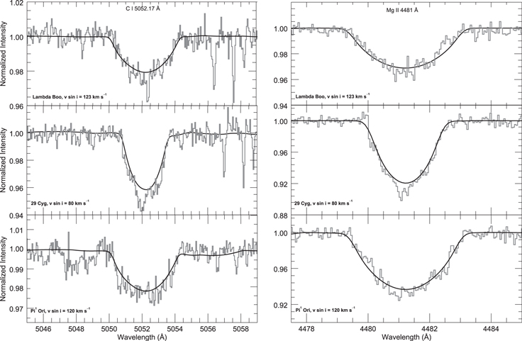
Figure 3. Observed visible spectra (ELODIE; gray lines) of Lambda Boo/HD 125162 (top; v sin i = 123 km s−1), 29 Cyg/HD 192640 (middle; v sin i = 80 km s−1), and Pi1 Ori/HD 31295 (bottom; v sin i = 120 km s−1) can be fit well by single-temperature synthetic spectra (black lines). All synthetic spectra have been convolved to the resolution of ELODIE data. The circumstellar absorption features in the line cores of 29 Cyg (middle panels) are not generally seen in the other stars. Strong telluric lines are visible redward of the C i 5052.17 Å feature; however, they are not included in our equivalent width measurement range. There is a weak telluric line near the center of the C i line, but we have determined that its contribution to both the equivalent width and the line ratio is negligible.
Download figure:
Standard image High-resolution imageHeiter (2002) used abundances of 34 Lambda Boo stars to construct a "mean" Lambda Boo abundance pattern. She concluded that the iron-peak elements from Sc to Fe as well as Mg, Si, Ca, Sr, and Ba are depleted by about 1.00 dex relative to the solar chemical composition (Al is 0.50 dex more depleted than Fe). The abundances of the light elements C, N, O, and S are around the solar values. In this study we use Heiter's "mean" Lambda Boo abundance pattern to create visible synthetic spectra of "average" Lambda Boo-type stars. The details of our modeling procedures can be found in Paper I (Cheng et al. 2016; Section 3).
4.2. Generating Synthetic "Model" Spectra
As discussed in Paper I, we generated a grid of synthetic spectra covering a wide range of temperature and metallicity in order to identify the best absorption lines to use for a diagnostic line ratio. These synthetic spectra also allow us to quantify the effects on equivalent width measurements due to spectral resolution, v sin i, blending, signal-to-noise ratio (S/N), and varying atmospheric parameters.
Using ATLAS910 and SPECTRUM,11 we then generated five sets of models (details can be found in Paper I) that are representative of:
- 1."Mean" Lambda Boo stars with [M/H] = −1.00 and elemental abundances as provided in Table 8 of Heiter (2002),
- 2."Normal" reference stars with solar abundances ([M/H] = 0.00) from Grevesse & Sauval (1998),
- 3."Normal" reference stars with [M/H] = 0.20,
- 4."Mildly metal-weak" stars with [M/H] = −0.50, and
- 5."Metal-weak" stars with [M/H] = −1.00.
For model sets three through five the elemental abundances are reduced by the given [M/H] values with respect to solar abundances.
All five sets of models were generated using a microturbulence velocity of 2.0 km s−1. Each model set includes subsets of models produced with:
- •log g = 3.50, 4.00, 4.50;
- •v sin i = 0, 50, 100, 150, 200, 250 km s−1; and
- •S/N = 50, 100, 200, 400, and no noise.
For each subset of models we generated 21 synthetic spectra with an effective temperature range of 6000–11,000 K in a step size of 250 K. These models cover the wavelength range 1000–10000 Å.
4.3. Absorption Line Selection
In Paper I, we demonstrated that the C i 1657 Å/Al ii 1671 Å equivalent width ratio can be used to distinguish between Lambda Boo stars and other metal-weak stars. However, it only works well for stars hotter than ∼8000 K, because cooler stars do not have much flux shortward of 1700 Å. It also requires the acquisition of ultraviolet spectra from a space-based telescope. Since more than half of all known Lambda Boo stars have  K (see Figure 4 and Table 1), we have searched for other equivalent width ratios in the visible wavelength range that can be used to classify cooler Lambda Boo stars.
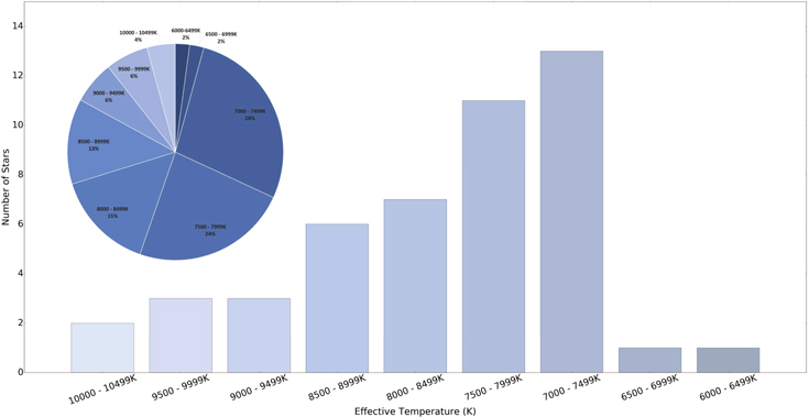
Figure 4. Effective temperature distribution of 47 program Lambda Boo stars with archival ELODIE and/or ESO data. 56% of them are cooler than 8000 K. Since these stars do not have enough flux shortward of 1700 Å, they cannot be classified by the UV criterion (C i 1657 Å/Al ii 1671 Å) specified in Paper I (Cheng et al. 2016).
Download figure:
Standard image High-resolution imageWe first explored the Mg ii 4481 Å/Fe i 4383.5 Å equivalent width ratio because this ratio has been used extensively in the literature to classify Lambda Boo stars (cf. Gray & Corbally 2009, ch. 5). After carefully analyzing the observed spectra of all of our program stars and synthetic spectra, however, we conclude that the Mg ii 4481 Å/Fe i 4383.5 Å equivalent width ratio does not discriminate Lambda Boo stars from normal stars with temperatures cooler than 9500 K when applied "quantitatively" (see Figure 5). Nevertheless, the Mg ii 4481 Å/Fe i 4383.5 Å ratio plays an important role in the discovery of Lambda Boo stars via visual classification techniques (see Section 5), as it was used to successfully discover and classify the "confirmed" Lambda Boo stars discussed in Murphy et al. (2015).
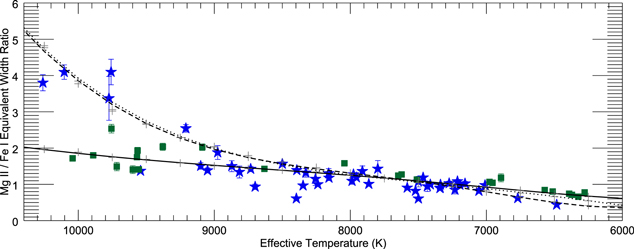
Figure 5. Mg ii 4481 Å/Fe i 4383.5 Å equivalent width ratio of Lambda Boo stars (blue star symbols), normal stars (green square symbols), and three sets of model spectra (with no noise or rotational broadening) as a function of effective temperature. The solid line indicates the "normal star" ([M/H] = 0.00) models. The model for the average Lambda Boo abundance pattern (dashed line; see Section 4.1) is almost identical to the [M/H] = −1.00 model (dotted line). Equivalent width ratio uncertainties (error bars representing the range of multiple measurements by several co-authors) are given for individual stars, but are not included for the "noise-free" models (indicated by "+" signs). A "mean" temperature for each star was derived from literature values. Temperature ranges for individual stars are given in Tables 1 and 2. The wavelength range used to measure the Mg ii 4481 Å feature is 4479.0–4483.5 Å. The wavelength range used to measure the Fe i 4383.5 Å feature is 4381.5–4385.8 Å. It is clear from this figure that the Mg ii 4481 Å/Fe i 4383.5 Å equivalent width ratio cannot be used to discriminate Lambda Boo stars from other metal-weak stars, or even from normal stars for effective temperatures below 9000 K. This ratio is, however, very useful in the discovery of Lambda Boo stars by "visual" spectral classification (see Section 5).
Download figure:
Standard image High-resolution imageLambda Boo stars have subsolar abundances of heavier elements but near-solar abundances of the lighter C, N, O, and S elements, so a diagnostic line ratio should be based on the relative strength of light and heavy elements. We explored various measurable lines in the wavelength range of 4000–6800 Å. Although this visible wavelength range is rich in absorption lines from the chemical elements we are interested in, weak lines and some blended features cannot be used because they cannot be accurately measured. Since more than 50% of our program Lambda Boo-type stars have projected rotational velocities over 100 km s−1 (Figure 2(b)), nearly all absorption features are blended to some extent. Our absorption line selection was done by examining both observed and synthetic spectra.
We found that the C i 5052.17 Å/Mg ii 4481 Å equivalent width ratio is the most useful line ratio for separating cooler Lambda Boo stars from normal stars and other metal-poor stars. It also helps to separate "strong" Lambda Boo-type stars from "mild" Lambda Boo-type stars. Both the C i and Mg ii lines are, of course, blended features (see Figures 6 and 7). There is some contamination in both features from nearby Fe i lines, and the amount of Fe i contamination varies with temperature (see Figure 8). We therefore carefully selected our equivalent width measurement wavelength ranges (see Table 4) to cover the primary line of interest with minimal and consistent amounts of contamination.
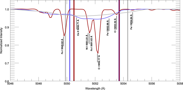
Figure 6. Fe i contamination present in our measurement of the C i 5052.17 Å feature using three models of an average Lambda Boo star with Teff = 7000 K (see Section 4.2) and v sin i = 0 km s−1 (red line), 100 km s−1 (blue line), and 200 km s−1 (gray line). The wavelength range of our equivalent width measurement depends on v sin i (see Table 4) and is denoted by vertical bars with colors corresponding to the associated models. These wavelength ranges were selected to ensure that we captured all of the equivalent width of the rotationally broadened C i 5052.17 Å line and the weaker C i 5053.52 Å line, while minimizing the amount of Fe i contamination for program stars with a range of v sin i values. All model spectra have been convolved to the resolution of ELODIE data.
Download figure:
Standard image High-resolution image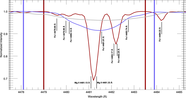
Figure 7. Fe i contamination present in our measurement of the Mg ii 4481 Å feature using three models of an average Lambda Boo star with Teff = 7000 K (see Section 4.2) and v sin i = 0 km s−1 (red line), 100 km s−1 (blue line), and 200 km s−1 (gray line). The wavelength range of our equivalent width measurement depends on v sin i (see Table 4) and is denoted by vertical bars with colors corresponding to the associated models. These wavelength ranges were selected to ensure that we captured all of the equivalent width of the rotationally broadened Mg ii lines while minimizing the amount of Fe i contamination for stars with different v sin i. All model spectra have been convolved to the resolution of ELODIE data.
Download figure:
Standard image High-resolution image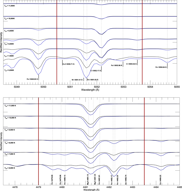
Figure 8. This figure illustrates that there is some contamination from the temperature-sensitive Fe i lines in both the C i 5052.17 Å (top) and Mg ii 4481 Å (bottom) equivalent width measurements, so the amount of Fe i contamination is Teff dependent. The black lines denote models of average Lambda Boo stars, and the blue lines denote models of "normal" ([M/H] = 0.00) stars. Both sets of models were generated with v sin i = 0 km s−1 and no noise to emphasize the absorption lines in this region. The wavelength ranges used for equivalent width measurements of stars and models with v sin i = 0 km s−1 are denoted by the vertical red bars (see Table 4). All model spectra have been convolved to the resolution of ELODIE data.
Download figure:
Standard image High-resolution imageTable 4. Selected Features
| Blended Feature | Component | Observed Wavelength1 |
|---|---|---|
| (Equivalent Width Measurement Range) | (Å) | |
| C i 5052.17 Å (Air) | Co ii | 5050.7096 |
| ([a] 5050.5–5053.7 Å for 0 km s−1≤v sin i < 25 km s−1; | Ni i | 5051.5065 |
| [b] 5050.5–5053.7 Å for 25 km s−1≤v sin i < 75 km s−1; | Fe i | 5051.6342 |
| [c] 5050.2–5053.7 Å for 75 km s−1 ≤v sin i < 125 km s−1; | C i | 5052.1673 |
| [d] 5049.9–5054.0 Å for 125 km s−1 ≤v sin i < 175 km s−1; | Fe i | 5052.9812 |
| [e] 5049.9–5054.3 Å for 175 km s−1 ≤v sin i < 225 km s−1; | C i | 5053.5153 |
| [f] 5049.7–5055.0 Å for v sin i ≥225 km s−1) | Fe i | 5054.6422 |
| Mg ii 4481 Å (Air) | Fe i | 4479.6032 |
| ([a] 4479.0–4483.5 Å for 0 km s−1≤v sin i < 25 km s−1; | Fe i | 4479.9622 |
| [b] 4478.6–4483.5 Å for 25 km s−1≤v sin i< 75 km s−1; | Fe i | 4480.1362 |
| [c] 4478.1–4483.9 Å for 75 km s−1≤v sin i < 125 km s−1; | Mg ii | 4481.1304 |
| [d] 4478.0–4485.1 Å for 125 km s−1≤v sin i < 175 km s−1; | Mg ii | 4481.3274 |
| [e] 4477.5–4485.2 Å for 175 km s−1≤v sin i < 225 km s−1; | Fe i | 4481.6092 |
| [f] 4476.5–4485.6 Å for v sin i ≥225 km s−1) | Fe I | 4482.1702 |
| Fe i | 4482.2522 | |
| Fe i | 4482.7392 | |
| Fe i | 4484.2202 | |
References. Kramida et al. (2014), (2) Nave et al. (1994), (3) Moore (1970), (4) Risberg (1955), (5) Kurucz & Bell (1995), (6) Pickering et al. (1998).
Download table as: ASCIITypeset image
4.4. Equivalent Width Measurements
We measured the equivalent widths of the C i 5052.17 Å and Mg ii 4481 Å absorption features (Table 4) of all our observed visible spectra and each of the model spectra. Each observed spectrum was individually wavelength-shifted to align with models of similar parameters (Teff, log g, [M/H], etc.). We performed the equivalent width measurements using autocfeature, which is a heavily modified version of the program feature in the IUEDAC IDL library.12 The details of our autocfeature program can be found in Paper I. Because the projected rotational velocity (v sin i) of the confirmed Lambda Boo stars ranges from 3 km s−1 to 267 km s−1, we also explored the effects of stellar rotation on the line profiles and our equivalent width measurements. Spectral lines that are broadened and blended due to rotation cannot be clearly separated (see Figures 6 and 7) using the standard equivalent width measurement method.
Because the equivalent width of the line is conserved under rotational broadening, we first adopted fixed wavelength ranges for measuring C i and Mg ii equivalent widths. We then utilized synthetic spectra to determine the optimal wavelength range for various v sin i values (see Table 4). This allowed us to balance the equivalent width lost from our lines of interest with the equivalent width gained from other nearby features. The temperature dependence of the blends (see Figure 8) makes this procedure unreliable for v sin i > 200 km s−1.
Figure 9 illustrates the use of our program autocfeature to measure the equivalent widths of a standard star's (HD 113139; v sin i ∼100 km s−1) C i 5052.17 Å and Mg ii 4481 Å absorption features. The equivalent width is defined as the area enclosed by the feature and a "pseudo-continuum" drawn through its highest points, therefore the "pseudo-equivalent width" heavily depends on how one chose the continuum. These "pseudo-equivalent widths" are useful only for an empirical classification but not for a detailed abundance analysis. We used the same procedure and a v sin i-dependent equivalent width measurement range to measure the equivalent widths of these two lines in every observed and synthetic spectrum. For each model and observed spectrum, several members of our team independently measured the equivalent widths of selected lines used in this study. From these measurements we determined internal error bars in order to quantify measurement repeatability. The equivalent width measurements of the model spectra were internally consistent to better than 2% (without noise or rotational broadening) and 7% (with S/N = 200 and various amounts of rotational broadening) for all selected features.
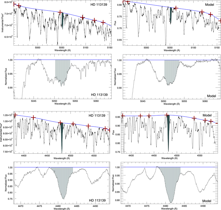
Figure 9. This figure illustrates the use of our program autocfeature (see Section 4.4) to measure the equivalent widths of the blended C i 5052.17 Å and Mg ii 4481 Å features in the standard star HD 113139's (v sin i ∼ 100 km s−1) ELODIE spectrum (left) and a model spectrum with similar stellar parameters (right). Our program performs a cubic spline interpolation between user-selected anchor points (red crosses) to fit the local continuum, divides by that continuum to normalize the visible spectrum, then calculates the equivalent width. The user's pre-selected equivalent width measurement wavelength ranges (values listed in Table 4) are then matched to the closest wavelength values in the "pseudo-continuum" to calculate the equivalent width (shaded regions). The same equivalent width measurement procedure was applied to all of the observed and synthetic spectra (with various levels of noise and various amounts of rotational broadening added) used in this work.
Download figure:
Standard image High-resolution image5. RESULTS
The primary goal of this paper is to establish a "quantitative" classification criterion that uses visible spectra to distinguish Lambda Boo stars from other stars with temperatures less than 8000 K. We measured the C i 5052.17 Å/Mg ii 4481 Å equivalent width ratios of all the "confirmed" Lambda Boo stars and "nonmember" stars listed in Murphy et al. (2015) that have archival ELODIE/ESO spectra.
Initially, we selected fixed wavelength ranges to measure the equivalent width of the absorption features (5050.0–5054.4 Å for C i and 4479.0–4483.5 Å for Mg ii). Our results using these fixed wavelength ranges to measure the C i and Mg ii equivalent widths in both observed spectra and noise-free comparison models without rotational broadening are illustrated in Figure 10. This equivalent width ratio has the highly desirable property that overall metal-weak stars have a smaller ratio than normal stars, and Lambda Boo stars have higher ratios. Equivalent width ratios of the observed spectra generally match the model predictions (see Figure 10). At temperatures cooler than 9500 K the differences among the normal star, average Lambda Boo-type star, and metal-weak star models are significant. At temperatures hotter than 9500 K, these models converge. For program stars with Teff values >10,000 K, the C i 5052.17 Å feature is too weak to perform an accurate measurement of its equivalent width (see Figure 8), so we exclude program stars with Teff > 10,000 K from Figure 10. Stars hotter than 8000 K can be discriminated by the C i 1657 Å/Al ii 1671 Å equivalent width ratio we presented in Paper I if UV spectra are available. For stars with effective temperatures between 8000 K and 9500 K, both the C i 1657 Å/Al ii 1671 Å and C i 5052.17 Å/Mg ii 4481 Å equivalent width ratios can be used together. The error bars shown in Figure 10 represent multiple independent measurements by various co-authors but do not compensate for effects such as inaccurate continuum placement due to random noise or for uncorrected telluric contributions to the ratio.
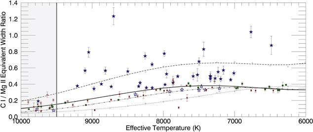
Figure 10. C i 5052.17 Å/Mg ii 4481 Å equivalent width ratio (measured using fixed equivalent width measurement ranges; see Section 5) of Lambda Boo stars (blue stars), normal stars (green squares), nonmembers (red circles), and four sets of model spectra (with no added noise or rotational broadening) as a function of effective temperature. The long dashed line indicates the models generated using the average Lambda Boo abundance pattern (see Section 4.2), the solid line indicates the "normal/reference star" [M/H] = 0.00 models, the dashed–dotted–dotted–dotted line indicates [M/H] = −0.50 models, and the dotted line indicates [M/H] = −1.00 models. Lambda Boo-type stars that fall below the "normal star" ([M/H] = 0.00) models and nonmember stars that fall above the "normal/reference star" models are denoted by unfilled symbols and listed in Table 5. Measurement uncertainties (error bars representing the range of multiple measurements by several co-authors) are given for individual stars' observed spectra, but are not included for the "noise-free" models (indicated by "+" signs; average model ratio error was less than 2%). A mean temperature for each star was derived from literature values. Temperature ranges for individual stars are given in Tables 1–3. At temperatures hotter than 9500 K the models converge (gray region), so the C i 5052.17 Å/Mg ii 4481 Å equivalent width ratio is no longer capable of clearly separating Lambda Boo-type stars from other metal-poor stars and normal stars.
Download figure:
Standard image High-resolution imageAs shown in Figure 10, the C i 5052.17 Å/Mg ii 4481 Å equivalent width ratio is an excellent quantitative diagnostic for cooler (<9500 K), unambiguous Lambda Boo stars. Of the 47 confirmed Lambda Boo stars listed in Table 1, seven stars cooler than 9500 K fall below the normal star models (see Table 5). Among them, four have been previously classified as mild Lambda Boo stars. Of the 43 nonmember stars listed in Table 3, five stars cooler than 9500 K fall above the normal star models (with [M/H] = 0 and solar abundances; see Table 5). We exclude one of those five nonmember stars (HD 89353, a post-AGB star; Kohoutek 2001) from Figure 10 because its ratio is much higher than the y-axis range due to its hyper-metal depletion ([Fe/H] = −4.7; Venn et al. 2014) but near-solar C, N, O, and S abundances (Mathis & Lamers 1992).
Table 5. Stars in Figure 10 with Unfilled Symbols
| Identificationa | Mean Teff | Teff Differenceb | [Fe/H] | [M/H] |
|---|---|---|---|---|
| (K) | (K) | |||
| Program Lambda Boo Stars | ||||
| HD 120500 (mild) | 8394 | −7/+7 | −0.67 | ... |
| HD 198160 | 7912 | −316/+169 | −0.850 | −1.00 |
| HD 193256 | 7739 | −653/+531 | −0.95 | ... |
| HD 139614 (mild) | 7500 | −100/+100 | −0.5 | ... |
| HD 218396 (mild) | 7465 | −110/+121 | −0.7 | −0.47 |
| HD 174005 | 7412 | −292/+325 | −0.20 | −0.77 |
| HD 120896 (mild) | 7213 | −194/+171 | −0.074 | −0.5 |
| Program Nonmember Stars | ||||
| HD 30739 | 9345 | −331/+175 | −0.20 | −0.10 |
| HD 142666 | 7867 | −367/+633 | −0.03 | −0.06 |
| HD 110377 | 7858 | −258/+270 | ... | −0.59 |
| HD 89353c | 7550 | −50/+50 | −4.7 | −5.0 |
| HD 108283 | 7282 | −112/+178 | −0.03 | −0.35 |
Notes.
aNote that these stars are listed in descending Teff order to assist with locating each star in Figure 10. bThe difference between the mean effective temperature and the lowest/highest effective temperature. cThis star is excluded from Figure 10 (see details in Section 5).Download table as: ASCIITypeset image
Having demonstrated that the C i 5052.17 Å/Mg ii 4481 Å equivalent width ratio can be used to clearly separate our three groups of program stars ("confirmed" Lambda Boo stars, normal/reference stars, and nonmember stars), we then performed an in-depth study to explore how v sin i, log g, and finite S/N affect our equivalent width measurements. Instead of using a fixed wavelength range to measure our program stars' equivalent width, we adopted v sin i-dependent wavelength ranges (see Table 4) and used the procedure described in Section 4.4. We also generated synthetic models with v sin i ranging from 0 to 250 km s−1 in increments of 50 km s−1. Each set of models has three subsets generated with log g = 3.50, 4.00, and 4.50, respectively (as shown in Figure 2(a), the average log g for our confirmed Lambda stars is ∼4.01). We also explored a range of S/N and found that random noise has little effect on the C i/Mg ii equivalent width ratio if S/N > 200. Because most of our program stars' observed spectra have S/N > 200, we added random noise corresponding to an S/N of 200 to all of our synthetic spectra and measured them using the same equivalent width measuring procedure we used to measure the equivalent widths of the C i 5052.17 Å and Mg ii 4481 Å absorption features in observed spectra.
The results of this in-depth analysis are illustrated in Figure 11. The shaded bands represent the overall envelope within which all of our models fall. While a Lambda Boo star may fall within the green band among models with abundances scaled uniformly from the solar abundances, this alone is not indicative that the star is not a Lambda Boo-type star. These bands illustrate the range of uncertainty when this diagnostic is applied to a sample of stars with undetermined stellar parameters. If v sin i has been determined for a particular sample star, this range of uncertainty can be reduced by using the revised wavelength ranges shown in Table 4. Ideally, each star should be compared to specific models with comparable stellar parameters. Figure 11 illustrates that our program Lambda Boo stars are still separated from normal and nonmember stars in a similar manner as illustrated in Figure 10, so our initial, simpler procedure provides a valid empirical diagnostic to separate most Lambda Boo stars from other metal-weak stars. For stars with v sin i > 200 km s−1, this ratio becomes highly uncertain, but most of our program stars are well below this threshold.

Figure 11. C i 5052.17 Å/Mg ii 4481 Å equivalent width ratio (measured using the v sin i-dependent measurement ranges listed in Table 4) of Lambda Boo stars (blue stars), normal stars (green squares), nonmembers (red circles), and 1575 model spectra as a function of effective temperature (covering a range of v sin i and log g, all with S/N = 200; see Sections 4.2 and 5). Each of the shaded color bands represents the overall envelope within which the associated models fall. These bands are formed by applying a polynomial fit to the minimum and maximum C i/Mg ii equivalent width ratios at each temperature and for each model set. The blue band (bounded by third-order polynomial fits) represents all data points contained in the "average" Lambda Boo star model set (model set #1) and the light purple band (bounded by fourth-order polynomials) represents all data points contained in the [M/H] = −1.00 model set (model set #5). The green band (bounded by fifth-order polynomials) represents all data points contained in the "normal" model sets (model sets #2 and #3), and the [M/H] = −0.50 model set (model set #5). As shown in Table 2, our program normal/reference stars have published [M/H] values ranging from +0.15 to −0.49 dex. Measurement uncertainties (error bars representing the range of multiple measurements by several co-authors) are given for individual stars' C i/Mg ii equivalent width ratio, but are not included for the models (indicated by "+" signs; average model ratio error was less than 7%). Mean temperatures and temperature uncertainties for individual stars are given in Tables 1–3. If a star falls within the green band among models with abundances scaled uniformly from solar abundances, this alone is not indicative that the star is not a Lambda Boo-type star. These stars should be compared to specific "normal/reference" star models with comparable stellar parameters. At temperatures hotter than 9500 K, the models converge (gray region), so the C i 5052.17 Å/Mg ii 4481 Å equivalent width ratio is no longer capable of clearly separating Lambda Boo-type stars from other metal-poor stars and normal stars.
Download figure:
Standard image High-resolution image
A long-standing problem in the classification of Lambda Boo stars is the status of apparent Lambda Boo stars with spectral types of F1 and later. Figure 4 shows the dramatic decrease in Lambda Boo frequency for spectral types later than F1 (Teff < 7000 K); this is presumably due to the mixing brought about by the development of a deep surface convection zone, which would erase the peculiar surface abundances of the Lambda Boo stars. Nonetheless, a number of potential Lambda Boo stars have been identified in the literature with spectral types (hydrogen-line types) as late as F3. A case in point is HD 106223, which has been classified as a field horizontal-branch star (Oke et al. 1966), a Lambda Boo star (Slettebak 1968), and a field blue straggler (Bond & MacConnell 1971). Gray (1988) classified this star as "F3 V kA1mA0 λ Boo?" but left the Lambda Boo status uncertain. More recent abundance determinations (Andrievsky et al. 2002; Heiter 2002) have shown an unambiguous Lambda Boo abundance pattern, with the carbon abundance near or even exceeding solar ( Heiter 2002), whereas the metals in general are about 1.5 dex below solar. Paunzen et al. (2014) also studied HD 106223 in their investigation of the possibility of an intrinsic chemical peculiarity in the Lambda Boo stars. It is thus of considerable interest that the C i 5052.17 Å/Mg ii 4481 Å classification criterion established in this paper clearly supports the Lambda Boo status of both HD 106223 and a similar star HD 4158 (see Table 1 and Figures 10 and 11). This illustrates the use of this criterion for separating late-type (F1 and later) Lambda Boo stars from metal-weak thick-disk early F-type stars.
We also investigated why the Mg ii 4481 Å/Fe i 4383.5 Å equivalent width ratio is useful in "visual" classification, but cannot be used as a "quantitative" diagnostic ratio (see Figure 5) in the same way that the C i 5052.17 Å/Mg ii 4481 Å ratio can be used. The Mg ii 4481 Å doublet goes through a maximum in strength in the late-B, early A-type stars (Teff ∼ 10,000 K), and declines in strength with decreasing temperature (see Figure 8). On the other hand, Fe i 4383.5 Å is a low-excitation line (∼1.5 eV), and thus grows in strength with declining temperature. This means that the Mg ii/Fe i ratio decreases with decreasing Teff in both normal and metal-weak stars. This is why, at a given temperature, the Mg ii 4481 Å/Fe i 4383.5 Å ratio has no power to discriminate between metal-poor and metal-rich stars (see Figure 5). It is important to note that in spectral classification, we often compare spectra of stars with quite different effective temperatures. This is the case with the Lambda Boo stars. A classifier confronted with the blue-violet spectrum of a "strong," cool Lambda Boo star will first consider the strength of the metallic-line spectrum and the Ca ii K-line, and note their similarity to the spectrum of an early A-type star, except for one inconsistency—the "peculiar" weakness of the Mg ii 4481 Å line (yielding a small Mg ii/Fe i ratio). Further investigation will show that the hydrogen lines have profiles more consistent with a late-A or even early F-type star, revealing the true Teff of the star and its general metal-weak nature. Once the Teff is known, it is clear that the Mg ii/Fe i ratio for the Lambda Boo star is not in fact unusual, but is nearly equal to that of a solar-metallicity standard star of the same effective temperature. Therefore the Mg ii/Fe i ratio plays an important role in the discovery of Lambda Boo stars via "visual" classification techniques, although it has little or no power in "quantitative" analysis to distinguish members of the class.
6. CONCLUSIONS
We studied 47 Lambda Boo stars with existing ELODIE and/or ESO visible spectra. We also analyzed model spectra of normal/reference stars, metal-poor stars, and "mean" Lambda Boo stars. We conclude that:
- 1.the visible spectra of Lambda Boo stars can be reproduced well with LTE synthetic spectra. These synthetic spectra can then be used to predict and explain the behavior of observed spectra as a function of stellar properties;
- 2.the C i 5052.17 Å/Mg ii 4481 Å equivalent width ratio can be used as a visible criterion to distinguish between Lambda Boo stars and other metal-weak stars. This ratio is a function of the individual star's effective temperature and [M/H]. Between 6000 K and 9500 K, the C i/Mg ii equivalent width ratios of Lambda Boo stars are very different from the C i/Mg ii ratios of normal star models and from other metal-poor stars;
- 3.this ratio can be used as an empirical diagnostic, even for a sample with unknown stellar parameters, by using "fixed" equivalent width measurement wavelength ranges (5050–5054.4 A for C i and 4479–4483.5 Å for Mg ii). If the star's v sin i is known, the power to discriminate Lambda Boo from normal stars and other metal-weak stars can be improved by using "v sin i-dependent" equivalent width measurement ranges;
- 4.we cannot use the C i 5052.17 Å/Mg ii 4481 Å equivalent width ratio as a classification criterion for stars hotter than 9500 K because their C i 5052.17 Å absorption features are too weak to be measured accurately;
- 5.we caution against using this equivalent width ratio as a classification criterion for stars with v sin i > 200 km s−1; and
- 6.one of the major advantages of establishing a visible Lambda Boo classification criterion is that archival visible data are widely available, and new visible observations are easier to obtain than UV observations.
Our future work will include:
- 1.performing an abundance analysis for program Lambda Boo stars without an abundance analysis present in the literature;
- 2.compiling an updated list of "bona fide" Lambda Boo stars that meet our quantitative visible and/or UV classification criteria, which can be used to investigate group properties in order to explain the origin of the Lambda Boo phenomenon.
This program is supported by grants from the National Science Foundation to California State University Fullerton (AST-1211213), the College of Charleston (AST-1211221, AST-1109695), and Appalachian State University (AST-1211215). Some of the data presented in this paper were obtained from the Mikulski Archive for Space Telescopes (MAST). STScI is operated by the Association of Universities for Research in Astronomy, Inc., under NASA contract NAS5-26555. Support for MAST for non-HST data is provided by the NASA Office of Space Science via grant NNX13AC07G and by other grants and contracts. Based on data obtained from the ESO Science Archive Facility under request numbers: djohnson 227337 and 240569. This research has made use of the SIMBAD database, operated at CDS, Strasbourg, France. This research has also made use of the VizieR catalogue access tool, CDS, Strasbourg, France.
Footnotes
- 6
- 7
- 8
MK standards can be found at http://www.pas.rochester.edu/~emamajek/spt/.
- 9
The "IUE Ultraviolet Spectral Atlas of Standard Stars" can be accessed at https://archive.stsci.edu/prepds/iuesass_web/iue.html.
- 10
Castelli and Kurucz' ATLAS9 program and LTE atmosphere models can be accessed from http://www.oact.inaf.it/castelli.
- 11
Gray's program SPECTRUM can be downloaded from http://www.appstate.edu/~grayro/spectrum/spectrum.html.
- 12
The original "feature.pro" program, as well as the rest of the IUEDAC library, can be found at https://archive.stsci.edu/iue/prolog.html.