


ABSTRACT
Parameters and abundances have been derived for 1002 stars of spectral types F, G, and K, and luminosity classes IV and V. After culling the sample for rotational velocity and effective temperature, 867 stars remain for discussion. Twenty-eight elements are considered in the analysis. The α, iron-peak, and Period 5 transition metal abundances for these stars show a modest enhancement over solar averaging about 0.05 dex. The lanthanides are more abundant, averaging about +0.2 dex over solar. The question is: Are these stars enhanced, or is the Sun somewhat metal-poor relative to these stars? The consistency of the abundances derived here supports an argument for the latter view. Lithium, carbon, and oxygen abundances have been derived. The stars show the usual lithium astration as a function of mass/temperature. There are more than 100 planet-hosts in the sample, and there is no discernible difference in their lithium content, relative to the remaining stars. The carbon and oxygen abundances show the well-known trend of decreasing [x/Fe] ratio with increasing [Fe/H].
Export citation and abstract BibTeX RIS
1. INTRODUCTION
This paper is one of a series (Heiter & Luck 2003; Luck & Heiter 2005, 2006, 2007; Luck 2015) that seeks to determine the standard of normalcy of the local region, regarding stellar abundances. The local region, in this context, is a Sun-centered sphere with a radius of approximately 100 parsecs. What is sought in the abundance data are reliable trends in the metal content of stars due to spatial, temporal, or stellar characteristic variations. Assuming the local region is a typical volume, these results should be applicable as a metric in further explorations of galactic chemical evolution. This hope has been borne out with the use of these results in the GAIA benchmark stars (Blanco-Cuaresma et al. 2014; Heiter et al. 2015; Jofré et al. 2015).
Numerous analyses have considered dwarfs in the local region. Hinkel et al. (2014) assembled the dwarf studies into a critically considered abundance database called the Hypatia Catalog. From the abundances found therein, they discussed the nucleosynthetic history of the local region. More recent studies have considered dwarf abundances and parameters in terms of the Li-problem in planet-host versus non-hosts (for example—Gonzalez 2014, 2015). Dwarf abundances further afield have been determined for stars with planets detected by the Kepler satellite (Schuler et al. 2015).
One of the problems associated with the assembly of a critically considered catalog of abundances, such as the Hypatia Catalog, is the question of systematic differences among various abundance sources. Abundance differences can arise from systematic stellar parameter differences, differences in atomic data—especially in damping constants and oscillator strengths—and things as mundane as choice of model atmosphere source and line analysis code. A better way to overcome these problems, rather than trying to allow for the differences, is a self-consistent analysis of a large sample of local dwarfs. Such an analysis is the concern of this work.
The 216 dwarfs of Luck & Heiter (2006) are the starting point for this study. An additional 469 dwarfs were observed using the McDonald Observatory Struve Telescope and Sandiford Echelle Spectrograph. For the analysis, 624 of these stars were retained, with the bulk of the eliminated dwarfs found to be double-line spectroscopic binaries. An additional 57 dwarfs were added to the sample from data obtained using the Hobby–Eberly Telescope and its High-Resolution Spectrograph. These stars were observed as radial velocity standards during the Cepheid study of Luck & Lambert (2011). Lastly, 360 dwarfs were extracted from the ELODIE Archive. The total number of dwarfs is 1002, as there is some overlap between the Hobby–Eberly data and the other two data sets. Basic data for the program stars can be found in Table 1, along with quantities such as distance and absolute magnitude. Also indicated are the 108 dwarfs in this sample that are planet hosts. The planets are all close giant planets; that is, super-Jupiters in orbits within 0.5 AU of the host.
Table 1. Program Stars
| Primary | HD | HIP | HR | CCDM | Spectral Type | P | e_P | V | d | E(B–V) | Mv | Host |
|---|---|---|---|---|---|---|---|---|---|---|---|---|
| (mas) | (mas) | (mag) | (pc) | (mag) | (mag) | |||||||
| ksi UMa B | 98230 | ⋯ | 4374 | J11182+3132B | G2V | 113.20 | 4.60 | 4.73 | 8.8 | 0.00 | 5.00 | ⋯ |
| HD 179958 | 179958 | ⋯ | 7294 | J19121+4951A | G2V | 40.16 | 0.83 | 6.57 | 24.9 | 0.00 | 4.59 | ⋯ |
| HD 179957 | 179957 | ⋯ | 7293 | J19121+4951B | G3V | ⋯ | ⋯ | 6.75 | ⋯ | 0.00 | 4.77 | ⋯ |
| BD-10 3166 | ⋯ | ⋯ | ⋯ | ⋯ | K3.0V | 15.34 | 3.08 | 10.01 | 65.2 | 0.00 | 5.94 | H |
| 85 Peg | 224930 | 171 | 9088 | ⋯ | G5V_Fe-1 | 82.17 | 2.23 | 5.75 | 12.2 | 0.00 | 5.32 | ⋯ |
| HD 225239 | 225239 | 394 | 9107 | ⋯ | G2V | 25.52 | 3.28 | 6.11 | 39.2 | 0.00 | 3.14 | ⋯ |
| HD 38A | 38A | 473 | ⋯ | J00057+4548A | K6V | 85.10 | 2.74 | 8.83 | 11.8 | 0.00 | 8.48 | ⋯ |
| HD 79211 | 79211 | 120005 | ⋯ | J09144+5241B | K7V | 156.45 | 8.58 | 7.72 | 6.4 | 0.00 | 8.69 | ⋯ |
Note. Information in the first nine columns from SIMBAD. CCDM is the Catalog of Double and Multiple Stars. P = parallax in milliarcseconds. e_P = error in parallax in milliarcseconds. V = Johnson V apparent magnitude. d = distance in parsecs. E(B–V) = B–V color excess, computed from the extinction method of Hakkila et al. (1997). Except for d < 75 pc, the extinction is set to 0. Mv = Johnson V band absolute magnitude. Host = Planet host status—H = known host. Source is The Extrasolar Planets Encyclopedia (Exoplanets team 2016).
Only a portion of this table is shown here to demonstrate its form and content. A machine-readable version of the full table is available.
Download table as: DataTypeset image
2. OBSERVATIONAL MATERIAL AND EQUIVALENT WIDTH DETERMINATION
The McDonald Observatory 2.1 m Telescope and Sandiford Cassegrain Echelle Spectrograph (McCarthy et al. 1993) provided much of the observational data for this study. High-resolution spectra were obtained during numerous observing runs, from 1996 to 2010. The spectra cover a continuous wavelength range from about 484 to 700 nm, with a resolving power of about 60,000. The wavelength range used demands two separate observations—one centered at about 520 nm, and the other at about 630 nm. Typical S/N values per pixel for the spectra are more than 150. Cancellation of telluric lines was achieved using broad-lined B stars that were regularly observed with S/N exceeding that of the program stars. The extraction process is identical to that detailed in Luck (2015).
Spectra of 57 dwarfs were obtained using the Hobby–Eberly telescope and High-Resolution Spectrograph. The spectra have a resolution of 30,000, spanning the wavelength range of 400 to 785 nm. They also have very high signal-to-noise ratios, >300 per resolution element in numerous cases. The reduction of these spectra follows the process detailed in Luck & Lambert (2011).
The last set of spectra were obtained from the ELODIE Archive (Moultaka et al. 2004). These spectra are fully processed, including order co-addition, and have a continuous wavelength span of 400 to 680 nm and a resolution of 42,000. The ELODIE spectra utilized here all have S/N > 75 per pixel.
In the tables that detail the analysis results (Tables 3–5), stars observed with the Sandiford spectrograph are denoted "S" in the "Sp" column. Similarly, stars from the HET and High-Resolution Spectrograph are indicated by "H," and the objects from the ELODIE Archive are designated by an "E."
Processing of the spectra was performed using an interactive graphics package developed by the author. The software enables Beer's law removal of telluric lines, smoothing with a fast Fourier transform, continuum normalization, and wavelength setting. Two changes have been made in spectrum reduction, relative to the procedures found in Luck (2014, 2015). The first is that order co-addition for Sandiford echelle spectra has been implemented; second, the equivalent width routine has been upgraded to better account for the wings of stronger lines.
After continuum placement and wavelength scale (photospheric) determination, the Sandiford orders are co-added using weights drawn from smoothed flat fields. This process yields excellent relative intensities, along the orders and from order to order. The order co-addition minimizes S/N variations due to the blaze function, leaving only the modest S/N variation due to detector response over the 140 nm total spectral window. The co-add proceeds by determining the order-to-order overlap in wavelength space, places the overlap regions on a common wavelength scale, and then co-adds, using (w1*n1 + w2*n2)/(w1 + w2) as the co-added value. The weights for the point in the two respective orders are w1 and w2, whereas n1 and n2 are the continuum-normalized intensities. The wavelength scale step for the co-added data is not constant along the spectrum. The values change periodically, to mimic the original wavelength steps.
Stellar line profiles are set by the Voigt function—a convolution of a Gaussian and a Lorentz profile. In low-density environments, such as found in giants and supergiants, line profiles are primarily Gaussian up to equivalent widths of about 25 nm. They are easily and accurately measured using the Gaussian approximation: EW = 1.06 * Depth * Full Width at Half Maximum (FWHM), where the depth is measured relative to the normalized continuum. Unfortunately, in solar-type dwarfs, the lines have more prominent contributions from the Lorentz part of the profile, and the Gaussian approximation begins to fail at about 7.5 nm in equivalent width. The precise point at which the observed profile deviates significantly from a Gaussian depends on the rotation velocity and the resolution of the observation. Rotational velocities of up to about 15 to 20 km s−1 deviate little from a pure Gaussian, and slit profiles are usually considered also to be Gaussian. For example, consider a line with a true equivalent width of 9.49 nm, as determined from a direct integration of a theoretical profile derived using a solar model. Convolving that profile with 1.0 km s−1 of rotation and a slit resolution of 60,000, and then using the Gaussian approximation to determine the equivalent width, one obtains 8.98 nm. If the rotation is increased to 5 km s−1, the same exercise yields 9.17 nm for the equivalent width. For a resolution of 42,000 and the same rotation values, the Gaussian equivalent width values are 9.04 and 9.16 nm, respectively. As the equivalent width increases, the Gaussian approximation increasingly undershoots the actual equivalent width.
How can one overcome this problem? One possibility is to use direct integration on the observed profiles. Although this is feasible for the Sun, and is the usual practice, it is not realistic to attempt this for thousands of lines in hundreds of stars. Another way forward might be to try to fit a Voigt profile to the lines, using nonlinear least squares to derive the fitting parameters. This technique was investigated in the Sun, and turns out to need direct human interaction because the solutions tend to be rather unstable and often diverge, giving bad fits. Another problem with the nonlinear least squares approach is that one needs the derivatives of the function to be fitted; for the Voigt function, the derivatives are non-trivial.
The way forward from this point is to adopt the function known as the pseudo-Voigt function—a linear combination of a Gaussian and an exponential function. The function is:
where a is the amplitude/depth of the feature, x0 is the central wavelength, x is the wavelength of interest, b is related to the half-width at half-maximum depth (HWHM), and c specifies the relative contribution from the two generating functions. For c = 0, one has a pure Gaussian and b is the HWHM. A pure exponential is found at c = 1, where b = 0.849 * HWHM. For any value of c, there is a unique solution for b as a function of HWHM.
A virtue of the pseudo-Voigt approach is that the derivatives are easily computed, and the profile is computationally simple. Implementing nonlinear least squares fit using this function for theoretical profiles shows that excellent profile fits are obtained up to equivalent widths of over 40 nm, at resolutions up to 120,000 and rotations approaching 20 km s−1. However, when the nonlinear least square procedure is applied to the Sun, the approach suffers from instabilities in the solutions due to impinging blends.
A better way to handle the problem is to use a chi-square minimization approach. One first determines the depth and HWHM of the feature to be fitted. One then cycles through a series of c values, and for each chosen c, computes b from the relation between b and the HWHM for that c. After computing each pseudo-Voigt profile, the chi-square statistic is calculated. The c giving minimum chi-square is judged to be the best fit. Comparing the best-fit chi-square b and c values to those derived from nonlinear least squares for "clean" solar lines and theoretical profiles show excellent correspondence, with the benefit that the chi-square is not prone to numerical instability.
Applying the chi-square technique to stellar spectra is possible, but the lower resolution and signal-to-noise limit its direct application. A number of spectra were reduced using the chi-square minimization technique, but the number of lines yielding a good minimum was inadequate. What was noticed is that the values of c that were found varied in step with the Gaussian equivalent width and overall line width; i.e., with rotational velocity. This behavior points to a usable path: given the rotational speed and resolution, one can construct a relation between the Gaussian equivalent width and the required value of c, based on theoretical profiles. Then, given the rotational velocity of a star, one can obtain a working relation between c and Gaussian equivalent widths. For our program stars, the rotational velocity was obtained using synthetic spectra to fit the region around 570 nm, the best fitting velocity (and spectrum resolution) was then used to interpolate the Gaussian equivalent width–c relation for the star.
Equivalent widths were measured using the Gaussian approximation and the pseudo-Voigt function. Specifically, one first determines the Gaussian equivalent width, then one obtains c using that one. Next, one uses the observed HWHM and c to obtain b. Finally, using those values of b and c along with the observed depth, one generates the pseudo-Voigt profile and integrates it to find the equivalent width. For most lines, the difference in the Gaussian equivalent width and the pseudo-Voigt equivalent width is small—at 10 nm, the difference is typically 0.5 nm, whereas at 20 nm, the difference is 2 nm. For this analysis, an upper equivalent width limit of 20 nm was imposed. The average equivalent width used in the analysis is 7 to 9 nm.
3. ANALYSIS
3.1. Line list and Analysis Resources
The line list used here is the same as used in and described by Luck (2014, 2015). Briefly, the line list consists of about 2900 lines with solar oscillator strengths. Many of these lines have been used in solar abundance analyses, whereas others have been shown to be unblended. The equivalent widths used to determine the oscillator strengths were determined using direct integration during an interactive examination of each line in the Delbouille et al. (1973) solar intensity atlas. Thus, the line list can provide excellent abundances in solar-type dwarfs. As one goes further away from the solar temperature, coincident wavelength blends become more problematic; however, the line list provides a firm basis for the analysis, because unblended lines in the Sun have a better chance of being free of contaminants at other temperatures than do most lines. The line measurement process makes sure that the wavelength of the line to be measured falls at the proper wavelength relative to the wavelength of the desired line. This process eliminates strong blends from nearby lines. The sifting process applied during abundance determination further trims the initial list by removing less obvious blends.
The solar oscillator strengths adopt the solar abundances of Scott et al. (2015a, 2015b) and Grevesse et al. (2015) for species with an atomic number greater than 10. Van der Waals damping coefficients are taken from Barklem et al. (2000) and Barklem & Aspelund-Johanson (2005), or computed using the van der Waals approximation (Unsöld 1938). Hyperfine data for Mn, Co, and Cu from Kurucz (1992) were also utilized. The MARCS solar atmosphere (Gustafsson et al. 2008) was used for all calculations. This model uses plane-parallel geometry with effective temperature 5777 K and log g = 4.44. The adopted microturbulence was 0.8 km s−1.
Abundances for all program stars were calculated using plane-parallel MARCS model atmospheres (Gustafsson et al. 2008). An interpolation code developed by the author was used to interpolate at the desired parameters. Tests indicate the code can accurately reproduce grid models to within 5 K in temperature, and the remaining structure to within 1%–2%. Stellar metallicity is taken into account in the analysis by using the model grid closest in metallicity to the target star. Above [M/H] = −1, the grid spacing is 0.25 dex in metallicity and extends up to +0.25 dex. Thus, the model metallicity is generally within 0.125 dex of the star itself. The line calculations were made using the LINES and MOOG codes (Sneden 1973), as extended and maintained by R. Earle Luck since 1975.
3.2. Stellar Parameters and Z > 10 Abundances
The photometric calibration of Casagrande et al. (2010) was used for effective temperature determination. Photometry was obtained using the General Catalog of Photometric Data (Mermilliod et al. 1997), 2MASS photometry (Cutri et al. 2003) from SIMBAD, uvby photometry from Paunzen (2015), and Tycho photometry from the Tycho-2 catalog (Høg et al. 2000). The line of sight extinctions were determined using the code of Hakkila et al. (1997) and adopting distances computed using Hipparcos parallaxes (van Leeuwen 2007). The Hakkila et al. code uses (l, b, d) versus AV relations to determine AV. The extinction within 75 pc of Sun is essentially nil (e.g., Vergely et al. 1998; Leroy 1999; Sfeir et al. 1999; Breitschwerdt et al. 2000; Lallement et al. 2003). The extinctions (and reddenings) of all stars within 75 pc were thus set to zero. For stars lying beyond 75 pc, the extinction out to 75 pc was subtracted from the total extinction. The parallax uncertainty of these stars or systems has a median value of 2%. Secondary stars without determined parallaxes are assumed to lie at the same distance as the primary in the system. The absolute V magnitudes are mostly good, to the ±0.1 mag level.
All available colors were utilized for the initial temperature determination. The [Fe/H] values used in the Casagrande et al. (2010) calibration were taken from Luck & Heiter (2006), the Hypatia database (Hinkel et al. 2014), the PASTEL database (Soubiran et al. 2010), or assumed to be solar. The individual effective temperature values were examined if the standard deviation of the mean exceeded 100 K. Obvious outliers were eliminated from the final average. Colors involving 2MASS magnitudes were examined more closely for the brightest stars, due to possible saturation effects in the photometry. It was found that, if there was a temperature outlier, it most often was V–J, where J is the 2MASS J magnitude. For that reason, the V–J color was eliminated from the effective temperature determination for all stars. Table 2 gives the photometric temperature, its standard deviation, and the number of colors utilized. These temperatures are well determined on the whole: the mean standard deviation of the temperature for the stars is 48 K. The number of temperatures utilized is 8 to 9 in the mean. However, there are a few cases that are not so well defined, with the worst case being α Cep (HR 8218), which shows a range of 700 K over the three colors retained. There is no obvious reason for the spread. The mean temperature for this star and the other five stars with a standard deviation more than 150 K are consistent with their spectral types; thus, they remain in the data set, but their parameters and abundances are not on the same level of reliability as the others.
Table 2. Temperature, Luminosity, Mass, Age, and Gravity
| B1 | D | Y | B2 | |||||||||||||||
|---|---|---|---|---|---|---|---|---|---|---|---|---|---|---|---|---|---|---|
| Primary | Sp | T | Sig | N | log L/LS | Mass | Age | Mass | Age | Mass | Age | Mass | Age |

|
Range |

|
Range | log g |
| (K) | (K) | (MS) | (Gyr) | (MS) | (Gyr) | (MS) | (Gyr) | (MS) | (Gyr) | (MS) | (MS) | (Gyr) | (Gyr) | cm s−2 | ||||
| 10 CVn | S | 5987 | 90 | 9 | 0.01 | 0.94 | 6.31 | 0.86 | 8.00 | 0.94 | 5.42 | 0.90 | 7.12 | 0.91 | 0.08 | 6.71 | 2.58 | 4.44 |
| 10 Tau | S | 6014 | 83 | 11 | 0.49 | 1.02 | 7.94 | 0.97 | 9.00 | 1.33 | 3.00 | 1.02 | 7.75 | 1.09 | 0.36 | 6.92 | 6.00 | 4.05 |
| 107 Psc | S | 5259 | 55 | 9 | −0.36 | 0.91 | 1.62 | 0.89 | 1.18 | 0.89 | 2.33 | 0.88 | 2.09 | 0.89 | 0.03 | 1.80 | 1.15 | 4.58 |
| 109 Psc | S | 5604 | 46 | 7 | 0.46 | 1.01 | 9.47 | 1.11 | 7.75 | 1.05 | 8.50 | 1.07 | 8.42 | 1.06 | 0.10 | 8.53 | 1.72 | 3.94 |
| 11 Aql | S | 6144 | 29 | 7 | 1.18 | ⋯ | ⋯ | 1.47 | 2.25 | 1.78 | 1.80 | 1.61 | 1.50 | 1.62 | 0.31 | 1.85 | 0.75 | 3.57 |
| 11 Aqr | S | 5929 | 52 | 8 | 0.31 | 1.18 | 2.51 | 1.17 | 4.50 | ⋯ | ⋯ | 1.18 | 4.63 | 1.18 | 0.01 | 3.88 | 2.11 | 4.24 |
| 11 LMi | S | 5498 | 48 | 9 | −0.09 | 0.98 | 4.50 | 1.00 | 4.36 | 1.00 | 4.50 | 0.95 | 9.27 | 0.98 | 0.05 | 5.66 | 4.91 | 4.43 |
| 110 Her | S | 6457 | 52 | 7 | 0.79 | ⋯ | ⋯ | 1.20 | 4.33 | ⋯ | ⋯ | 1.36 | 2.83 | 1.28 | 0.16 | 3.58 | 1.50 | 3.94 |
| 111 Tau | S | 6184 | 23 | 3 | 0.22 | 1.14 | 1.93 | 1.11 | 2.79 | 1.16 | 1.41 | 1.13 | 2.03 | 1.14 | 0.05 | 2.04 | 1.38 | 4.38 |
| 111 Tau B | S | 4576 | 32 | 9 | −0.77 | ⋯ | ⋯ | 0.75 | 0.83 | 0.71 | 7.50 | 0.74 | 0.96 | 0.73 | 0.04 | 3.10 | 6.67 | 4.66 |
| V* V566 Oph | E | 6358 | 60 | 5 | 0.59 | 1.18 | 4.36 | 1.02 | 6.90 | ⋯ | ⋯ | 1.12 | 4.83 | 1.11 | 0.16 | 5.36 | 2.54 | 4.05 |
Notes:
| Column | Unit | Description | ||
|---|---|---|---|---|
| Sp | N/A | Source for spectroscopic material | ||
| T | K | Effective Temperature | ||
| Sig | N/A | Standard deviation of the effective temperature | ||
| N | N/A | Number of colors used in the effective temperature determination | ||
| logL/Ls | Solar | Luminosity in logarithmic solar units | ||
| B1 | Mass | Solar | Mass in solar units, determined from the Bertelli et al. (1994) isochrones | |
| Age | Gyr | Age in gigayears, determined from the Bertelli et al. (1994) isochrones | ||
| D | Mass | Solar | Mass in solar units, determined from the Dotter et al. (2008) isochrones | |
| Age | Gyr | Age in gigayears, determined from the Dotter et al. (2008) isochrones | ||
| Y | Mass | Solar | Mass in solar units, determined from the Demarque et al. (2004) isochrones | |
| Age | Gyr | Age in gigayears, determined from the Demarque et al. (2004) isochrones | ||
| B2 | Mass | Solar | Mass in solar units, determined from the BaSTI Team (2016) isochrones | |
| Age | Gyr | Age in gigayears, determined from the BaSTI Team (2016) isochrones | ||

|
Solar | Average mass in solar masses | ||
| Range | Solar | Range in mass determination | ||

|
Gyr | Average age in gigayears | ||
| Range | Gyr | Range in age determination | ||
| log g | cm s−2 | Surface acceleration, computed from average mass, temperature, and luminosity. |
Only a portion of this table is shown here to demonstrate its form and content. A machine-readable version of the full table is available.
Download table as: DataTypeset image
Given the effective temperature, absolute magnitude, and mass, the surface acceleration due to gravity (e.g., the gravity) can be found. Isochrones were taken from Bertelli et al. (1994), Demarque et al. (2004), Dotter et al. (2008), and the BaSTI group (BaSTI Team 2016), and used to obtain the mass, age, and luminosity for each star. The fitting process is identical to that of Allende Prieto & Lambert (1999), which has been used subsequently in a number of analyses; e.g., Luck & Heiter (2006, 2007) and Luck (2015). Isochrone fitting is also dependent on the metallicity of the star in question, and the same metallicities used in temperature determination were used here. The luminosity given in Table 2 is derived from the distance, apparent V magnitude, and the bolometric corrections of Bessell et al. (1998). Comparison of the these luminosities to those derived in the isochrone fits shows they agree to within 0.02 dex.
There are, at times, substantial differences in mass and age estimates between isochrone sets. For example, the mass estimates for η Ser vary from 1.32 to 2.07 solar masses. However, the median value of the range in the mass estimate is 0.08 MSun. This uncertainty is 10% of the mean mass. Over 80% of the sample has a range in isochrone masses of less than 20%. The mean mass from the Bertelli et al. isochrones is 1.09 solar masses, 1.05 solar masses from Dotter et al., 1.10 solar masses from Demarque et al., and 1.09 solar masses from the BaSTI group. Thus, the masses are well-determined. In Table 2, there are about 30 stars lacking a mass determination from any isochrone set. Examination of the temperatures and luminosities of these stars show that they tend to be lower-temperature and lower-luminosity objects, thus falling outside the isochrone grids. For these, a mass was estimated by plotting the average masses for the stars with determined values against their effective temperature—the relation found is quite well-defined. The temperature of the stars without isochrone determined masses can be used, with the mass–temperature relation yielding a reasonable mass estimate. Note that a 30% uncertainty in the mass yields an uncertainty in the log g value of ±0.15. At 10% uncertainty in mass, the variation in log g is ±0.05. The values of log g found here should be reliable.
The microturbulent velocity is obtained by demanding that the iron abundance, as determined from Fe i lines, show no dependence on equivalent width. The process used here is the same as described in Luck (2015). The Fe i data are examined in a statistical manner based on Gaussian fitting to the abundance distribution. The Fe ii data have an insufficient number of lines to proceed statistically, so cuts are derived based on the number of lines present. From this data examination, master cut lists are derived for Fe i and Fe ii. Before clipping, the number of Fe i lines is of order 700; after clipping, it is about 500. Fe ii lines typically number 40–60 before trimming and 30–50 afterward. After arriving at the final Fe i and Fe ii data for each star, the microturbulent velocity is tweaked to a final value. Other species are clipped in the same way as Fe ii, but no master cut lists are generated.
An imbalance exists between the total iron abundance as derived from Fe i and Fe ii. The sense is that the mass derived gravity is too large; that is, the Fe ii total iron abundance exceed the Fe i total iron abundance—see Figure 1, Top Panel. This problem can be rectified using an ionization balance. This process forces the ionized and neutral species to yield the same total abundance by using as the free parameter the gravity. This process is implemented by interpolating a small grid of models, and then determining the best-fit gravity and microturbulence together. Parameter confirmation was performed by interpolating a new model at the proper parameters. The iron data relations were recomputed to confirm the ionization balance, along with the lack of dependence of iron abundance on line-strength. The difference between the mass and ionization balance gravities is "small" in the temperature regime within 500K of solar temperature (see Figure 1 Bottom Panel), with a mean value of 0.06 dex. In that region, the average iron abundance difference between Fe i and Fe ii for the mass derived gravities is −0.02 dex.

Figure 1. Top Panel: the difference in Fe i and Fe ii total iron abundances as a function of effective temperature, as determined from the mass-derived gravity. Bottom Panel: the difference in gravity from the mass-derived value, minus the ionization balance determination. The limit at a difference of 1.0 dex reflects the maximum change allowed. The low-temperature differences of 0.0 dex signify the lack of Fe ii data.
Download figure:
Standard image High-resolution imageTable 3 includes parameters and iron abundance details—log εFe, σ, and number of lines for both Fe i and Fe ii. Information for both mass and ionization-balance derived gravities is presented. Average abundances for 25 elements with Z > 10 are in Table 4. For elements having more than one ionization stage available, the final average is the average of all retained lines. A number of elements have both neutral and first ionized species available; the final average for these elements is merely the average of all retained lines. Note that the Mn, Co, and Cu abundances have been computed, allowing for hyperfine structure. Details of all Z > 10 abundances—per species average, σ, and number of lines—can be found in the online -only data—Table 7.
Table 3. Parameter and Iron Data
| Mass-derived Gravity | Ionization Balance Gravity | ||||||||||||||||||
|---|---|---|---|---|---|---|---|---|---|---|---|---|---|---|---|---|---|---|---|
| Primary | Sp | T | G | Vt | Fe i | σ | N | Fe ii | σ | N | T | G | Vt | Fe i | σ | N | Fe ii | σ | N |
| (K) | (cm s−2) | (km s−1) | (log ε) | (log ε) | (K) | (cm s−2) | (km s−1) | (log ε) | (log ε) | ||||||||||
| 10 CVn | S | 5987 | 4.44 | 1.08 | 7.01 | 0.06 | 313 | 6.95 | 0.04 | 16 | 5987 | 4.57 | 0.84 | 7.02 | 0.07 | 313 | 7.02 | 0.04 | 16 |
| 10 Tau | S | 6013 | 4.05 | 1.48 | 7.41 | 0.06 | 354 | 7.38 | 0.06 | 26 | 6013 | 4.11 | 1.44 | 7.41 | 0.06 | 354 | 7.41 | 0.06 | 26 |
| 107 Psc | S | 5259 | 4.58 | 0.56 | 7.48 | 0.07 | 234 | 7.58 | 0.15 | 17 | 5259 | 4.38 | 0.80 | 7.45 | 0.07 | 234 | 7.46 | 0.14 | 17 |
| 109 Psc | S | 5604 | 3.94 | 1.22 | 7.59 | 0.06 | 401 | 7.57 | 0.06 | 19 | 5604 | 3.98 | 1.18 | 7.59 | 0.06 | 401 | 7.59 | 0.06 | 19 |
| 11 Aql | S | 6144 | 3.57 | 2.83 | 7.50 | 0.15 | 195 | 7.43 | 0.11 | 17 | 6144 | 3.74 | 2.78 | 7.50 | 0.15 | 195 | 7.50 | 0.12 | 17 |
| 11 Aqr | S | 5929 | 4.24 | 1.40 | 7.73 | 0.06 | 387 | 7.71 | 0.07 | 28 | 5929 | 4.30 | 1.33 | 7.74 | 0.06 | 387 | 7.74 | 0.07 | 28 |
| 11 LMi | S | 5498 | 4.43 | 1.32 | 7.74 | 0.07 | 400 | 7.84 | 0.13 | 24 | 5498 | 4.19 | 1.59 | 7.70 | 0.08 | 400 | 7.69 | 0.13 | 24 |
| 110 Her | S | 6457 | 3.94 | 2.37 | 7.56 | 0.13 | 252 | 7.52 | 0.10 | 24 | 6457 | 4.04 | 2.33 | 7.56 | 0.13 | 252 | 7.56 | 0.10 | 24 |
| 111 Tau | S | 6184 | 4.38 | 2.04 | 7.57 | 0.11 | 277 | 7.51 | 0.08 | 19 | 6184 | 4.51 | 1.91 | 7.58 | 0.11 | 277 | 7.58 | 0.08 | 19 |
| 111 Tau B | S | 4576 | 4.66 | 0.80 | 7.65 | 0.14 | 213 | 8.30 | 0.47 | 15 | 4576 | 3.66 | 1.40 | 7.21 | 0.15 | 213 | 7.36 | 0.49 | 15 |
| V* V566 Oph | E | 6358 | 4.05 | 2.80 | 6.66 | 0.53 | 14 | 7.43 | 0.05 | 2 | 6358 | 3.05 | 2.50 | 6.64 | 0.53 | 14 | 7.11 | 0.05 | 2 |
| Column | Count | Column | Unit | Description |
|---|---|---|---|---|
| 2 | Sp | Source for spectroscopic material | ||
| 3 | T | K | Effective Temperature | |
| 4 | G | cm s−2 | Logarithm of the surface acceleration (gravity), computed from average mass, temperature, and luminosity. | |
| 5 | Vt | km s−1 | Microturbulent velocity | |
| 6 | Fe i | log ε | Total iron abundance, computed from neutral iron lines. The solar iron abundance is 7.47 | |
| 7 | σ | Standard deviation of the neutral iron line abundances | ||
| 8 | N | Number of neutral iron lines used | ||
| 9 | Fe ii | log ε | Total iron abundance, computed from first ionization stage iron lines. The solar iron abundance is 7.47 | |
| 10 | σ | Standard deviation of the first ionization stage iron line abundances | ||
| 11 | N | Number of first ionization stage iron lines used | ||
| 12 | T | K | Effective Temperature | |
| 13 | G | cm s−2 | Logarithm of the surface acceleration (gravity), computed from ionization balance | |
| 14 | Vt | km s−1 | Microturbulent velocity | |
| 15 | Fe i | log ε | Total iron abundance, computed from neutral iron lines. The solar iron abundance is 7.47 | |
| 16 | σ | Standard deviation of the neutral iron line abundances | ||
| 17 | N | Number of neutral iron lines used | ||
| 18 | Fe ii | log ε | Total iron abundance, computed from first ionization stage iron lines. The solar iron abundance is 7.47 | |
| 19 | σ | Standard deviation of the first ionization stage iron line abundances | ||
| 20 | N | Number of first ionization stage iron lines used |
Note. Columns 2–11 comprise the mass-derived gravity results.
Columns 12–20 comprise the ionization balance gravity results.
The effective temperature is the same in both cases.
Only a portion of this table is shown here to demonstrate its form and content. A machine-readable version of the full table is available.
Download table as: DataTypeset image
Table 4. Z > 10 Abundances for Mass-derived Gravities
| Primary | Sp | T | G | Vt | Na | Mg | Al | Si | S | Ca | Sc | Ti | V | Cr | Mn | Fe | Co | Ni | Cu | Zn | Sr | Y | Zr | Ba | La | Ce | Nd | Sm | Eu |
|---|---|---|---|---|---|---|---|---|---|---|---|---|---|---|---|---|---|---|---|---|---|---|---|---|---|---|---|---|---|
| 10 CVn | S | 5987 | 4.44 | 1.08 | −0.51 | −0.33 | −0.39 | −0.39 | −0.23 | −0.35 | −0.26 | −0.33 | −0.45 | −0.43 | −0.61 | −0.46 | −0.35 | −0.46 | −0.55 | −0.59 | 0.19 | −0.50 | −0.49 | 0.27 | −0.33 | −0.20 | |||
| 10 Tau | S | 6013 | 4.05 | 1.48 | 0.04 | 0.06 | 0.02 | 0.00 | 0.03 | 0.02 | 0.05 | −0.01 | −0.07 | −0.03 | −0.11 | −0.06 | 0.01 | −0.06 | −0.11 | −0.02 | 0.23 | 0.01 | 0.03 | −0.08 | −0.08 | 0.05 | 0.09 | −0.11 | 0.13 |
| 107 Psc | S | 5259 | 4.58 | 0.56 | 0.08 | 0.06 | 0.13 | 0.04 | 0.48 | 0.07 | 0.14 | 0.18 | 0.24 | 0.13 | 0.16 | 0.02 | 0.09 | 0.11 | 0.25 | −0.03 | 0.30 | 0.23 | −0.07 | −0.04 | 0.29 | 0.28 | 0.56 | 1.23 | 0.30 |
| 109 Psc | S | 5604 | 3.94 | 1.22 | 0.24 | 0.31 | 0.29 | 0.19 | 0.30 | 0.21 | 0.17 | 0.16 | 0.11 | 0.18 | 0.21 | 0.12 | 0.12 | 0.15 | 0.30 | 0.06 | 0.39 | 0.10 | 0.14 | 0.05 | 0.30 | 0.24 | 0.20 | 0.46 | 0.43 |
| 11 Aql | S | 6144 | 3.57 | 2.83 | 0.35 | −0.18 | 0.27 | 0.14 | 0.14 | 0.17 | 0.07 | 0.15 | 0.04 | 0.12 | −0.04 | 0.02 | 0.17 | 0.03 | −0.35 | 0.09 | 0.76 | −0.02 | 0.20 | 0.00 | 0.11 | ||||
| 11 Aqr | S | 5929 | 4.24 | 1.40 | 0.53 | 0.33 | 0.35 | 0.32 | 0.37 | 0.32 | 0.38 | 0.31 | 0.32 | 0.33 | 0.38 | 0.26 | 0.34 | 0.34 | 0.34 | 0.28 | 0.53 | 0.35 | 0.37 | 0.09 | 0.44 | 0.40 | 0.52 | 0.50 | 0.62 |
| 11 LMi | S | 5498 | 4.43 | 1.32 | 0.52 | 0.41 | 0.45 | 0.36 | 0.61 | 0.36 | 0.32 | 0.34 | 0.39 | 0.37 | 0.48 | 0.28 | 0.35 | 0.36 | 0.40 | 0.29 | 0.43 | 0.37 | 0.16 | 0.14 | 0.61 | 0.46 | 0.55 | 1.46 | 0.63 |
| 110 Her | S | 6457 | 3.94 | 2.37 | 0.26 | −0.15 | 0.25 | 0.15 | 0.21 | 0.22 | 0.12 | 0.20 | 0.33 | 0.09 | 0.04 | 0.09 | 0.40 | 0.08 | −0.30 | 0.43 | 0.18 | 0.75 | 0.18 | 0.22 | 0.60 | 0.20 | 0.67 | 0.42 | |
| 111 Tau | S | 6184 | 4.38 | 2.04 | 0.26 | 0.17 | 0.17 | 0.14 | 0.17 | 0.19 | 0.24 | 0.19 | 0.27 | 0.16 | 0.01 | 0.09 | 0.33 | 0.09 | −0.32 | 0.33 | 0.26 | 0.63 | 0.28 | 0.27 | 0.39 | 0.27 | 0.56 | ||
| 111 Tau B | S | 4576 | 4.66 | 0.80 | 0.36 | 0.28 | 0.08 | 0.37 | 1.13 | 0.39 | 0.20 | 0.16 | 0.28 | 0.27 | 0.21 | 0.22 | 0.31 | 0.21 | 0.24 | 0.59 | 0.69 | 0.19 | −0.20 | 0.19 | 0.83 | 1.46 | 1.37 | 2.01 | 0.42 |
| V* V566 Oph | E | 6358 | 4.05 | 2.80 | −0.92 | −0.19 | 0.48 | 1.87 | 1.05 | 0.84 | 0.82 | 0.28 | −0.71 | 0.77 | 0.39 | 1.20 | 4.57 | 0.31 | 0.84 | 0.19 | 0.36 | 0.60 | |||||||
| Column | Units | Designation | Description |
|---|---|---|---|
| Sp | N/A | N/A | Source for spectroscopic material. |
| T | K | Teff | Effective Temperature. |
| G | cm s−2 | log g | log of the surface acceleration due to gravity. |
| Vt | km s−1 | Vt | Microturbulent velocity. |
| Na | Solar | [Na/H] | The abundance of sodium, given logarithmically with respect to the solar value. |
| Mg | Solar | [Mg/H] | The abundance of magnesium, given logarithmically with respect to the solar value. |
| Al | Solar | [Al/H] | The abundance of aluminum, given logarithmically with respect to the solar value. |
| Si | Solar | [Si/H] | The abundance of silicon, given logarithmically with respect to the solar value. |
| S | Solar | [S/H] | The abundance of sulfur, given logarithmically with respect to the solar value. |
| Ca | Solar | [Ca/H] | The abundance of calcium, given logarithmically with respect to the solar value. |
| Sc | Solar | [Sc/H] | The abundance of scandium, given logarithmically with respect to the solar value. |
| Ti | Solar | [Ti/H] | The abundance of titanium, given logarithmically with respect to the solar value. |
| V | Solar | [V/H] | The abundance of vanadium, given logarithmically with respect to the solar value. |
| Cr | Solar | [Cr/H] | The abundance of chromium, given logarithmically with respect to the solar value. |
| Mn | Solar | [Mn/H] | The abundance of manganese, given logarithmically with respect to the solar value. |
| Fe | Solar | [Fe/H] | The abundance of iron, given logarithmically with respect to the solar value. |
| Co | Solar | [Co/H] | The abundance of cobalt, given logarithmically with respect to the solar value. |
| Ni | Solar | [Ni/H] | The abundance of nickel, given logarithmically with respect to the solar value. |
| Cu | Solar | [Cu/H] | The abundance of copper, given logarithmically with respect to the solar value. |
| Zn | Solar | [Zn/H] | The abundance of zinc, given logarithmically with respect to the solar value. |
| Sr | Solar | [Sr/H] | The abundance of strontium, given logarithmically with respect to the solar value. |
| Y | Solar | [Y/H] | The abundance of yttrium, given logarithmically with respect to the solar value. |
| Zr | Solar | [Zr/H] | The abundance of zirconium, given logarithmically with respect to the solar value. |
| Ba | Solar | [Ba/H] | The abundance of barium, given logarithmically with respect to the solar value. |
| La | Solar | [La/H] | The abundance of lanthanum, given logarithmically with respect to the solar value. |
| Ce | Solar | [Ce/H] | The abundance of cerium, given logarithmically with respect to the solar value. |
| Nd | Solar | [Nd/H] | The abundance of neodymium, given logarithmically with respect to the solar value. |
| Sm | Solar | [Sm/H] | The abundance of samarium, given logarithmically with respect to the solar value. |
| Eu | Solar | [Eu/H] | The abundance of europium, given logarithmically with respect to the solar value. |
Only a portion of this table is shown here to demonstrate its form and content. A machine-readable version of the full table is available.
Download table as: DataTypeset image
3.3. Li, C, and O Analysis
Lithium, carbon, and oxygen abundances were derived for the program stars by spectrum synthesis. The atomic line data—for Li i at 670.7 nm, C i at 505.2 and 538.0 nm, and O i at 615.5 nm and [O i] at 630.0 nm—used is the same as detailed in Luck (2015). The major change made in this analysis is in the line list for the region 507.5 to 518.5 nm that includes lines from the C2 Swan system. A new line list was extracted from the VALD database including molecular lines of C2, CN, MgH, CH, OH, and TiO. The molecular lines of primary importance are those of C2, as there is scant evidence for the presence of other molecular species above about 4250 K. The C2 data in VALD derives from Brooke et al. (2013), and comparison with the previously used constants in Luck (2015)—excitation potentials and oscillator strengths—shows excellent agreement. Illustrations of syntheses, such as those carried out here, can be found in Luck & Heiter (2006) for some of the same stars and spectra. Carbon and oxygen abundances below Teff = 4325 K are not given, due to blends making line detection unreliable for all carbon and oxygen indicators in the observed spectral regions.
Lithium LTE abundance data are presented in Table 5, including an indicator noting if the "abundance" should be considered an upper limit. Upper limits are those stars in which the observed lithium feature has a depth of two percent or less. There is no evidence for 6Li in any of these stars, and thus the syntheses do not include this species. Corrections for non-LTE effects in lithium from Lind et al. (2009) are also included.
Table 5. Lithium, Carbon, and Oxygen Data
| Primary | Sp | T | G | Vt | Vr | Fe | Li | NLTE | L | 505.2 | 538.0 | C2 | 615.5 | 630.0 | C | O |
|---|---|---|---|---|---|---|---|---|---|---|---|---|---|---|---|---|
| (K) | (cm s−2) | (km s−1) | (km s−1) | (log ε) | (log ε) | (log ε) | (log ε) | (log ε) | (log ε) | (log ε) | (log ε) | (log ε) | ||||
| 10 CVn | S | 5987 | 4.44 | 1.08 | 3.9 | 7.01 | 2.04 | 0.04 | ⋯ | 7.78 | 7.86 | 8.03 | 8.64 | 8.66 | 7.89 | 8.65 |
| 10 Tau | S | 6013 | 4.05 | 1.48 | 6.0 | 7.41 | 2.42 | 0.04 | ⋯ | 8.27 | 8.29 | 8.43 | 8.79 | 8.72 | 8.31 | 8.75 |
| 107 Psc | S | 5259 | 4.58 | 0.56 | 2.5 | 7.48 | 0.52 | 0.09 | L | 8.21 | 8.42 | 8.51 | 8.73 | 8.82 | 8.38 | 8.80 |
| 109 Psc | S | 5604 | 3.94 | 1.22 | 5.1 | 7.59 | 1.94 | 0.07 | ⋯ | 8.41 | 8.54 | 8.49 | 8.70 | 8.69 | 8.48 | 8.69 |
| 11 Aql | S | 6144 | 3.57 | 2.83 | 28.2 | 7.50 | 1.88 | 0.03 | L | 8.18 | 8.28 | ⋯ | 8.80 | 8.70 | 8.23 | 8.75 |
| 11 Aqr | S | 5929 | 4.24 | 1.40 | 5.7 | 7.73 | 2.43 | 0.04 | ⋯ | 8.61 | 8.61 | 8.71 | 9.00 | 8.88 | 8.64 | 8.91 |
| 11 LMi | S | 5498 | 4.43 | 1.32 | 4.7 | 7.74 | 0.60 | 0.07 | L | 8.55 | 8.66 | 8.67 | 9.04 | 8.91 | 8.62 | 8.94 |
| 110 Her | S | 6457 | 3.94 | 2.37 | 18.0 | 7.56 | 1.14 | 0.01 | L | 8.21 | 8.30 | ⋯ | 8.88 | ⋯ | 8.25 | 8.88 |
| 111 Tau | S | 6184 | 4.38 | 2.04 | 17.0 | 7.57 | 2.95 | 0.03 | ⋯ | 8.31 | 8.29 | 8.33 | 8.91 | 8.79 | 8.31 | 8.85 |
| 111 Tau B | S | 4576 | 4.66 | 0.80 | 4.4 | 7.65 | −0.02 | 0.14 | ⋯ | ⋯ | ⋯ | 8.94 | ⋯ | 9.10 | 8.94 | 9.10 |
| V* V566 Oph | E | 6358 | 4.05 | 2.80 | 48.7 | 6.66 | 2.20 | 0.01 | L | 6.96 | 7.47 | ⋯ | 8.69 | ⋯ | 7.21 | 8.69 |
| Sp | Source for spectroscopic material | ||||||
| T | K | Effective Temperature | |||||
| G | cm s−2 | Logarithium of the surface acceleration (gravity), computed from average mass, temperature, and luminosity. | |||||
| Vt | km s−1 | Microturbulent velocity | |||||
| Vr | km s−1 | Rotational velocity | |||||
| Fe | log ε | Iron abundance. The solar iron abundance is 7.47 relative to H = 12. | |||||
| Li | log ε | Lithium abundance. The solar lithium abundance is 1.0 dex | |||||
| NLTE | Correction for non local thermodynamic equilibrium | ||||||
| L | L = Upper limit on lithium abundance | ||||||
| 505.2 | log ε | Carbon abundance from C i 505.2 nm line. | |||||
| 538.0 | log ε | Carbon abundance from C i 538.0 nm line. | |||||
| C2 | log ε | Carbon abundance from C2 Swan lines—primary indicator at 513.5 nm | |||||
| 615.5 | log ε | Oxygen abundance from [O i] 630.0 nm line | |||||
| 630.0 | log ε | Oxygen abundance from O i 615.5 triplet | |||||
| C | log ε | Mean carbon abundance—weights discussed in text | |||||
| O | log ε | Mean oxygen abundance—weights discussed in text |
Only a portion of this table is shown here to demonstrate its form and content. A machine-readable version of the full table is available.
Download table as: DataTypeset image
The individual carbon features are combined as follows: for Teff < 5250 K, only C2 513.5 nm is used. At 5250 < T < 6000 K, C i 505.2 and 538.0 nm have weight 1 as does C2 513.5. For 6000 K < T < 6350 K, the two C i lines have weight 2, and C2 has weight 1. Above Teff > 6350 K, the two C2 are not used and the two C i lines have equal weight. Relative strength and blending are the basis for the weights. A typical range in abundance for the features is 0.15 dex. The Asplund et al. (2009) carbon abundance, log εC = 8.43, is adopted for the solar reference abundance. Table 5 has the per line/feature carbon data, as well as the average values.
Oxygen abundance indicators were averaged in the following manner: for Teff < 5250 K, [O i] only is used. For 5250 K < Teff < 6000 K, O i has weight 1 and [O i] has weight 3. In the regime 6000 K < Teff < 6350 K, O i and [O i] have equal weight. Lastly, for Teff > 6350 K only O i is used. Near the solar temperature, typical differences between oxygen derived from O i and [O i] are of order 0.15 dex. For Teff < 5500 K, the C–O interlock has been taken into account in the abundance determination. The oxygen data per line and averages are found in Table 5.
3.4. Abundance and Parameter Inspection
3.4.1. Internal Examination
Thirty-nine of the HET stars are in common with the remainder of the sample—31 with the Sandiford data and 8 with the ELODIE data. The temperatures and mass-derived gravities for the stars are the same. The HET data has the same wavelength extent as the ELODIE data, but extends further blue-ward than does the Sandiford data. This extended blue coverage means that there are more and different Fe i and Fe ii lines in the HET data than can be found in the Sandiford data, but approximately the same as found in the ELODIE data. The difference in the Fe i average abundance is +0.05 for HET—Sandiford; that is, the lower resolution HET data yields a higher abundance on the average. For HET versus ELODIE, the difference in Fe i is +0.02, on average. For Fe ii, the differences are +0.12 and −0.04, respectively. However, the individual standard deviations about the HET means for the Fe i data sets are in the range of 0.05 to 0.10 dex, whereas the Fe ii data has somewhat larger standard deviations, typically 0.1 to 0.15 dex. The offset between the different data sources is only marginally significant, especially for Fe i. In the Fe ii data, the offset in the HET—Sandiford comparison most likely lies in the fact that the number of Fe ii lines in the HET data averages twice the number found in the Sandiford data. The difference in number stems from the extended blue coverage of the HET data. The bluer Fe ii lines are likely to be more blended than the red lines in the Sandiford data, and thus give a somewhat higher total iron abundance. In the discussion that follows this section, the only HET data retained are the 18 unique HET stars. The abundances derived from the entire set of 57 HET stars, however, can be found in the abundance tables (Tables 3–5).
Other instances of equivalent width problems can be found in Figure 2 (top panel), where the ratios [S/Fe], [Si/Fe], and [Ni/Fe] versus temperature are shown. The data shown are derived using the mass-determined gravities. It is immediately evident that, below 4500 K, the S and Si data are not reliable; their ratios rapidly increase as a function of temperature. The most extreme case is [S/Fe], increasing from about 0 at 4750 K to +2 dex at 4000 K. Such an increase is not reasonable in any scenario of galactic or stellar evolution.
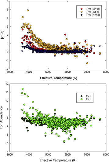
Figure 2. Top Panel: [S/Fe], [Si/Fe], and [Ni/Fe] vs. effective temperature for the program stars. The data shown are derived using the mass determined gravities. It is immediately evident that, below 4500 K, the S and Si data are not reliable because the ratios rapidly increase as a function of temperature. The most likely explanation is the intrusion of significant blends with decreasing temperature. Bottom Panel: Fe i and Fe ii total iron abundances as a function of temperatures. The Fe ii data are also affected by significant blend problems below 4500 K.
Download figure:
Standard image High-resolution imageThe source of the increase evidenced by the S i data in Figure 2 is growing blends in the weak higher excitation potential lines. A blend, in this case, means anything that causes the direct equivalent width measurement to provide an unreliable value. The cause of the blend can be a direct wavelength coincident with another line. However, more probable is that the line to be measured is perturbed by a nearby strong line(s) that can affect the depth, the central wavelength, the measured half-width, or all of these quantities. This behavior means that the lines are increasingly difficult to measure reliably. This problem is evidenced by the number of lines used as a function of temperature. The mean number of S i lines used over all stars is five, with the largest number being about twelve around an effective temperature of 6000 K. As the temperature decreases to 4500 K, the number of S i lines measured drops to about three. The blends keep the S i equivalent width constant, or even increasing with decreasing temperature for these lines.
The trend noted in S i is also the case for Si i. For Si i, the average number of lines is 39; however by 4500 K in effective temperature, the number of lines falls to about 30, and by 4000 K to less than 20. This is not because the lines are becoming too strong, but because blends make them difficult to identify reliably. For Ni i, the increase is not nearly so dramatic, but the abundances are still problematic below 4500 K. Here, the same behavior in numbers of lines applies. At 6000 K, there are about 170 lines, but by 4500 K the number decreases to about 50. The larger number of lines at 4500 K does yield better discrimination of heavily blended lines, but some evidence for the problem remains.
The bottom panel of Figure 2 returns to the iron data, showing the total iron abundance as derived from the mass-determined gravity for both Fe i and Fe ii. Below 4500 K, the Fe ii data shows the same problem as found in the S and Si data—there is a rapid increase in total iron content. This increase is responsible for the behavior seen in Figure 1. The reason for the increase in Fe ii is the same as that for the S i and Si i behavior—blends are severely affecting the data below 4500 K. The better path forward from this point is to consider, in the bulk of the discussion, only those stars with effective temperatures greater than 4500 K.
3.4.2. External Comparison
In consulting the PASTEL database (Soubiran et al. 2010), one finds that about 85% of the program stars analyzed here have previous determinations of stellar parameters and/or abundances. The number of references totals 371, spanning over six decades of work. With a median number of five references per analyzed star, the corpus of the analyses is massive and well beyond a succinct synopsis. For comparison purposes here, only a subset of post-2005 studies is considered. The primary results of the comparison are located in Table 6, where effective temperature, gravity, and [Fe/H] differences are given. Note that two gravities and [Fe/H] values are given. These correspond to the two gravity, and hence [Fe/H], determinations performed here.
Table 6. Parameter and Iron Abundance Comparison
| Study | N | Ttype | Gtype |

|
s_T |

|
s_G1 |

|
s_G2 |

|
s_Fe1 |

|
s_Fe2 |
|---|---|---|---|---|---|---|---|---|---|---|---|---|---|
| This vs. LH2006 | 207 | E | Ion | −74 | 116 | −0.09 | 0.27 | −0.17 | 0.22 | 0.00 | 0.10 | −0.04 | 0.12 |
| This vs. C+2010 | 74 | IRFM | Var | 2 | 52 | 0.02 | 0.19 | ⋯ | ⋯ | ⋯ | ⋯ | ⋯ | ⋯ |
| This vs. C+2011 | 612 | Var | Var | −23 | 97 | −0.03 | 0.09 | −0.08 | 0.24 | 0.02 | 0.12 | 0.00 | 0.13 |
| This vs. R+2013 | 211 | E | Ion | 22 | 76 | −0.06 | 0.18 | 0.04 | 0.10 | 0.02 | 0.22 | −0.02 | 0.25 |
| This vs. R+2014 | 30 | E | Ion | −8 | 57 | −0.07 | 0.05 | −0.07 | 0.15 | 0.01 | 0.03 | 0.01 | 0.03 |
| This vs. B+2014 | 100 | E | Ion | −21 | 100 | −0.04 | 0.13 | −0.06 | 0.17 | 0.00 | 0.07 | −0.01 | 0.08 |
| B+2014 vs. C+2011 | 642 | ⋯ | ⋯ | −24 | 105 | −0.01 | 0.14 | ⋯ | ⋯ | −0.02 | 0.14 | ⋯ | ⋯ |
| This vs. MM2012 | 15 | Var | A | 17 | 33 | −0.02 | 0.06 | −0.02 | 0.11 | 0.03 | 0.04 | 0.03 | 0.05 |
| This vs. C+2013 | 10 | Var | A | 26 | 61 | −0.02 | 0.04 | −0.03 | 0.15 | 0.00 | 0.08 | −0.01 | 0.09 |
| N | = number of common stars |
| T Type | = Method of effective temperature determination in comparison study. E = Excitation analysis IRFM = Infrared Flux Method Var = combination or literature derived |
| G Type | = Method of gravity determination in comparison study. Ion = spectroscopic ionization balance. Var = Combination (line wings/isochrones/literature). A = astroseimology |
| dT | = New effective temperature—Source |
| dG1 | = New Mass Gravity—Source |
| dG2 | = New Ionization Gravity—Source |
| dFe1 | = New Mass Gravity [Fe/H]—Source |
| dFe2 | = New Ionization Gravity [Fe/H]—Source |
| s_X | = Standard deviation of differences |
| Comparison Studies | |||||
| LH2006 | Luck & Heiter (2006) | R+2013 | Ramírez et al. (2013) | MM2012 | Morel & Miglio (2012) |
| C+2010 | Casagrande et al. (2010) | R+2014 | Ramírez et al. (2014) | C+2013 | Creevey et al. (2013) |
| C+2011 | Casagrande et al. (2011) | B+2014 | Bensby et al. (2014) | ||
Download table as: ASCIITypeset image
Table 7. [x/H] Detail for Z > 10: Physical Parameters
| Column # | Column | Description |
|---|---|---|
| 1 | Pri | Primary Name for the star |
| 2 | ID | Id tag for the star |
| 3 | Sp | Source of spectra |
| 4 | Teff | Effective Temperature (K) |
| 5 | Log(g) | Log surface gravity (cm/s2) |
| 6 | Vt | Microturbulent velocity (km/s) |
| 7 | [Na i/H] | Mean abundance of Na i relative to the solar value |
| 8 | Standard Deviation of the abundance about the mean | |
| 9 | N | Number of lies used in the mean abundance |
| 10–114 |

|
Columns 10–114 repeat the Na i sequence for |
| Mg i, Al i, Si i, Si ii, S i, Ca i, Ca ii, Sc i, Sc ii, Ti i, Ti ii, V i, | ||
| V ii, Cr i, Cr ii, Mn i, Fe i, Fe ii, Co i, Ni i, Cu i, Zn i, Sr i, Y i, | ||
| Y ii, Zr i, Zr ii, Ba ii, La ii, Ce ii, Pr ii, Nd ii, Sm ii, Eu i, Eu ii |
Only a portion of this table is shown here to demonstrate its form and content. A machine-readable version of the full table is available.
Download table as: DataTypeset image
The data presented in Table 6 indicate good consistency between the various analyses, whether or not they use traditional techniques such as a spectroscopic excitation and ionization balance technique for parameter determination (Ramírez et al. 2013, 2014; Bensby et al. 2014), or the latest astroseismology results (Morel & Miglio 2012; Creevey et al. 2013). Typical average differences in temperature scales are about 20 K, gravities vary by about ±0.05 dex, and abundances agree in the mean to about ±0.05 dex.
It is encouraging that the temperatures derived here, using the Casagrande et al. (2010) effective temperature scale, agree with the IRFM temperatures used to develop that scale—the mean difference is 2 K over 74 stars. However, the spread in the individual temperature determinations, as expressed in the standard deviation of the mean differences, is discouraging. The standard deviations are of order 50 to 100 K, which means that, in larger comparisons, the effective temperature differences range up to 500 Kelvin or more. This problem is evidenced in the Casagrande et al. (2011) and Bensby et al. (2014) comparisons with the current data. To determine if the problem is solely within this analysis, the differences between Casagrande et al. (2011) and Bensby et al. (2014) were also determined, with the results being very similar to those found in this work and those two studies.
Errors in effective temperatures in an excitation analysis can stem from equivalent width errors or systematic errors in oscillator strengths as a function of excitation potential. The latter is not a significant problem at this time, but equivalent width problems can be. The general sense is that weaker lines are prone to overestimation in equivalent width, whereas strong lines in dwarfs are susceptible to underestimates due to missing contributions from the wings. These errors can skew the potential–abundance relation, as well as the equivalent width–abundance relation, giving rise to erroneous effective temperatures and microturbulent velocities.
Photometric effective temperature determinations also have their problems. Photometric errors, for example; i.e., errors in calibration or saturation of bright sources, are possible. Here, a more pernicious problem is a confusion of multiple sources in the photometry aperture. Examination of Table 1 shows that many of these stars are doubles or multiples. Care must be taken to ensure that the star observed spectroscopically is the star that was observed photometrically. Great attention was focused here on source identification, but it still possible that source confusion remains. Source confusion means not only identification of the proper object, but also unresolved sources blending into the desired source. Source confusion is not only a problem for this study, but also for any large-scale work depending on photometry. A good example of this is the local neighborhood study of 16,000+ stars by Casagrande et al. (2011).
The importance of non-local thermodynamic equilibrium (NLTE) in the determination of iron abundances has been investigated starting with the work of Tanaka (1971) and proceeding to the current day. The dwarf analysis of Bensby et al. (2014) includes NLTE corrections in their iron data, but they note that the corrections are small. The data in Table 6 reflect this conclusion—the LTE iron abundances derived here agree very well with their NLTE values, and any differences correlate closely with differences in effective temperature. For the parameter range of interest here, the differences between LTE and NLTE iron abundances are <0.1 and often near 0 (Lind et al. 2012), consistent with the Bensby et al. result.
As the last point of comparison, the analysis of Ramírez et al. (2013) derives not only stellar parameters and iron abundances; it also derives oxygen abundances from the O i 777.5 nm triplet using an NLTE analysis. In this work, oxygen abundances have been derived from the [O i] 630.0 mn line and the 615.7 nm O i triplet using a pure LTE analysis. Comparison of the derived abundances yields an average difference of +0.02 dex for the mass-derived gravities derived here, and −0.02 dex for the ionization-based gravities. The standard deviation of the mean difference is 0.23 dex using 211 common stars. By eliminating nine discrepant stars, the mean differences change to +0.03 and 0.00 dex respectively, and the standard deviation falls to 0.17 dex. The agreement is excellent, considering the weakness of the lines used here.
4. DISCUSSION
Extended discussion of the nucleosynthetic history of the local region of the Milky Way can be found in Nomoto et al. (2013) and Hinkel et al. (2014). Correlations between local abundances and kinematics have been discussed recently by Bensby et al. (2014). The reader is referred to those works for greater detail than given here, where the focus is on what this study can say over and above earlier discussions.
4.1. Sample and Analysis Pruning
Figure 3 shows an HR diagram of the program stars. The sample is broken into subsets based on rotational velocity and proximity to the main sequence. The dividing line for rotational velocity is 20 km s−1. The velocity is set based on the ability to measure equivalent widths accurately, using the method described in Section 2; above 20 km s−1, the method fails to reproduce the profiles accurately. The division into dwarfs and non-dwarfs is relatively arbitrary; stars above the indicated line are far enough from the main sequence that they are likely subgiants, with perhaps a few stars still evolving toward their main sequence. What is to be investigated is if there are any plausible systematic differences between the dwarfs and non-dwarfs. A priori, no abundance differences would be expected, based on closed-box galactic chemical evolution and standard stellar evolution.

Figure 3. The HR diagram for the program stars. The sample is broken into subsets, based on rotational velocity and proximity to the main sequence. The dividing line for rotational velocity is 20 km s−1. The proximity division is the solid line indicated. Stars below the line are considered dwarfs, whereas those above are, except for one, subgiants.
Download figure:
Standard image High-resolution imageAnother sample pruning applied going forward is that stars with an effective temperature less than 4500 K are not usually considered in the discussion. The temperatures and mass-derived gravities are reliable, but the ionization gravity and overall abundances are suspect due to significant blending problems in these stars. Note that Figure 2 does indicate that iron abundances derived from Fe i below 4500 K are consistent—they show no significant dependence on temperature down to about 4000 K. The problem is that other elements/species with abundances determined from many fewer lines are not as reliable.
Although Table 3 gives parameters and iron abundance data for both the mass-derived and ionization balance-derived gravity, the abundances to be discussed are be drawn from the mass-derived gravity only. This selection is because, in limiting the temperature to be above 4500 K, the differences in the two gravities are small—averaging 0.11 dex, which means that the neutral and ionized derived total abundances are also in relatively good agreement. For Fe i versus Fe ii, the difference is −0.05 over 867 stars. In this comparison, the stars with high rotation velocities have been removed, but no discrimination made between the dwarfs and non-dwarfs.
4.2. Z > 10 Abundances
One of the more common ways to examine abundances is to plot mean abundances for the sample as a function of atomic number. In Figure 4, such a plot is shown. The data in this plot are the mean values for those stars with [Fe/H] > −0.4, rotational velocity <20 km s−1, and Teff > 4500 K. The [x/Fe] ratios are computed from the abundances given in Table 4. Both neutral and first ionized species are available for Si, Sc, Ti, V, Fe, Y, Zr, and Eu. The abundance given in Table 4 is the mean over all retained lines. For the Z = 56 elements other than Eu, only the first ionized species is available. Because the number of Fe i lines is much greater than the number of Fe ii lines, the mean iron abundance is essentially the mean Fe i abundance. To investigate if this causes differences in the [x/Fe] ratios, the ratios [x i/Fe i] and [x ii/Fe ii] were computed and found to not be significantly different from the ratios generated using the abundances in Table 4.
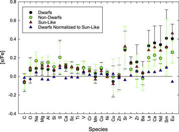
Figure 4.
![$\langle [{\rm{x}}/\mathrm{Fe}]\rangle $](https://content.cld.iop.org/journals/1538-3881/153/1/21/revision1/ajaa4df5ieqn11.gif) vs. element. The offsets from [x/Fe] are discussed in Section 4.2.
vs. element. The offsets from [x/Fe] are discussed in Section 4.2.
Download figure:
Standard image High-resolution imageThe sample has been subdivided based on the dwarf versus non-dwarf criteria from the preceding subsection. The iron-peak elements for both sub-samples have ![$\langle [{\rm{x}}/\mathrm{Fe}]\rangle $](https://content.cld.iop.org/journals/1538-3881/153/1/21/revision1/ajaa4df5ieqn12.gif) values of about +0.07 dex with a standard deviation of also about 0.07 dex; that is, as expected, they have close to the solar ratio of abundance relative to iron.
values of about +0.07 dex with a standard deviation of also about 0.07 dex; that is, as expected, they have close to the solar ratio of abundance relative to iron.
The elements Na, Mg, Al, and Si in the dwarfs show [x/Fe] values comparable to those found in for the iron-peak. Once again, this equality is as expected, because the lower abundance cut in iron eliminates most of the α-enhanced stars. What is surprising is that the non-dwarf stars have ![$\langle [{\rm{x}}/\mathrm{Fe}]\rangle $](https://content.cld.iop.org/journals/1538-3881/153/1/21/revision1/ajaa4df5ieqn13.gif) ratios that are systematically higher than what is found in the dwarfs. The effect is small, about 0.06 dex, and the one-sigma error bars do overlap with [x/Fe] = 0 as well as the dwarfs.
ratios that are systematically higher than what is found in the dwarfs. The effect is small, about 0.06 dex, and the one-sigma error bars do overlap with [x/Fe] = 0 as well as the dwarfs.
For the heavy elements with Z > 56, the situation is that, relative to the dwarfs, the non-dwarfs systematically have lower mean abundances. The offset, in this case, is somewhat larger (about 0.15), but the star-to-star abundances more scattered, which translates to the one-sigma error bars overlapping.
The overall offset from solar [x/Fe] ratios leads to the question of the behavior of the subset of dwarfs that have properties close to that of the Sun. The subset of such stars—34 in all with Teff within 100 K of the Sun—is shown in Figure 4 as red triangles. The error bars have been omitted, but they are comparable to the others shown. What is obvious is that these stars show a similar abundance pattern to that of the total sample. If one normalizes the total dwarf sample [x/Fe] ratios to these values, the result is the blue triangles in Figure 4. Unsurprisingly, the resulting ratios are close to zero.
Another way of examining abundances is to look for trends versus [Fe/H]. In Figure 5, the ratios [Si/Fe], [Ca/Fe], [Mn/Fe], [Ni/Fe], and [Zn/Fe] are shown as a function of [Fe/H]. The stars shown have been limited to −1 < [Fe/H]< +0.5. The trends in the data are well-known: silicon and calcium decrease with increasing [Fe/H] while [Mn/Fe] increases. Silicon and calcium are α-elements and their diminution as a function of [Fe/H] is due to the growing influence of Type Ia iron production with time. The enhancement of manganese with increasing [Fe/H] was first noted by Wallerstein (1962), and was commented upon by later authors (Gratton 1989; Feltzing et al. 2007; Luck & Heiter 2007; Luck 2015). Manganese is produced in Type Ia supernovae, and the observed trend is caused by the late onset of enrichment (Kobayashi & Nomoto 2009).
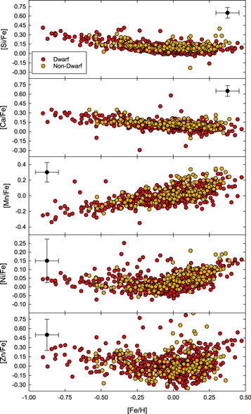
Figure 5. [Si/Fe], [Ca/Fe], [Mn/Fe], [Ni/Fe], and [Zn/Fe] vs. [Fe/H]. The trends exhibited in these panels are discussed in Section 4.2.
Download figure:
Standard image High-resolution imageThe nickel abundances show a very small spread in [Ni/Fe] in the region −1 < [Fe/H] < 0 (Figure 5, panel (d)) with a mean [Ni/Fe] ratio of near 0. At [Fe/H] ratios above solar, the [Ni/Fe] ratios increase to about [Ni/Fe] ∼ +0.1 at [Fe/H] ∼ +0.5. This behavior parallels the behavior in [Mn/Fe] (Figure 5, panel (c)), and is also found in the nickel data of Luck (2015) for local giants.
The zinc data shown in the bottom panel of Figure 5 indicates significant scatter at all [Fe/H] ratios. The scatter is not unexpected, as zinc abundances rest upon two lines, at most. Previous work has shown that the [Zn/Fe] ratios in the region −1 < [Fe/H] < −0.5 increases from about +0.07 dex to about +0.2 dex, and then falls back toward 0 at [Fe/H] = 0 (Saito et al. 2009). The overall features of the distribution found here are consistent with [Zn/Fe] ∼ 0 at all metallicities greater than [Fe/H] > −1, but nothing further can be said about them.
Two heavy element trends are shown in Figure 6. The top panels show neodymium, and the bottom two show europium. For each element, the top panel of the pair shows the sample, subdivided as dwarfs versus non-dwarfs, whereas the bottom plot of the pair keys the data based on effective temperature. Both plots that show the dwarfs versus the non-dwarfs are consistent with the non-dwarfs having lower [x/Fe] ratios, as indicated in Figure 4. Both neodymium and europium abundances are derived from ionized lines, and the lower gravity non-dwarfs have the stronger lines giving rise to a more secure abundance. The smaller spread in the non-dwarf heavy element abundances testifies to this difference. If one merely deletes any star with [Nd/Fe] > +0.6 dex from the ![$\langle [\mathrm{Nd}/\mathrm{Fe}]\rangle $](https://content.cld.iop.org/journals/1538-3881/153/1/21/revision1/ajaa4df5ieqn14.gif) ratio, the mean value for the dwarfs declines only marginally, and the non-dwarf ratio barely changes. The mean value of dwarf
ratio, the mean value for the dwarfs declines only marginally, and the non-dwarf ratio barely changes. The mean value of dwarf ![$\langle [{\rm{x}}/\mathrm{Fe}\rangle ]$](https://content.cld.iop.org/journals/1538-3881/153/1/21/revision1/ajaa4df5ieqn15.gif) ratios in all cases is being dominated by the sheer number of dwarfs with "normal" [x/Fe] ratios in the range −0.25 < [F/H] < +0.25.
ratios in all cases is being dominated by the sheer number of dwarfs with "normal" [x/Fe] ratios in the range −0.25 < [F/H] < +0.25.
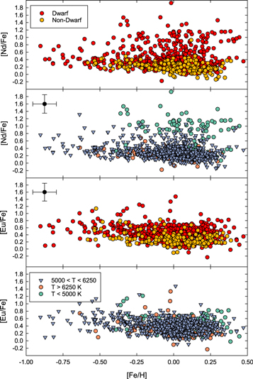
Figure 6. Top Panels: [Nd/Fe] vs. [Fe/H] and effective temperature. Bottom Panels: [Eu/Fe] vs. [Fe/H] and effective temperature. Although the Nd data appear influenced by the cooler stars (lower panel of Nd data), eliminating the outlying points has little effect upon the mean. The same is true for Eu.
Download figure:
Standard image High-resolution imageA question that has yet to be answered is why the [x/Fe] ratios for these stars are non-solar. Alternatively, one could ask—why are the Sun's elemental abundance ratios lower than those found in these stars? One could suspect the solar-derived transition probabilities used here, relative to laboratory values. Data for 519 of the Fe i lines used here can be found in the NIST database (Kramida et al. 2015). The mean difference in log gf is 0.02 dex (this work—NIST), with a standard deviation (σ) of 0.19. For Fe ii, the difference is 0.10 (n = 72, σ = 0.24). Looking at α- and other iron- peak elements, typical mean differences are 0.05 dex. The heavy elements show somewhat larger differences; for example, Nd ii has a mean difference of +0.1 dex. Such differences cannot explain the overabundances seen in the heavy elements mean [x/Fe] ratios. Another possibility would be differential effects between the solar model used to derive the gf values and the models used in the analysis. Differential model effects can be discounted because MARCS models were used for all analyses. Additionally, the solar-like stars show the same ![$\langle [{\rm{x}}/\mathrm{Fe}]\rangle $](https://content.cld.iop.org/journals/1538-3881/153/1/21/revision1/ajaa4df5ieqn16.gif) ratios as the total sample, indicating that something other than the models lies behind the high heavy element abundances. Two possibilities come to mind: (1) the ionized lines used for the analysis are severely affected by NLTE, or (2) the small sample of lines available for heavy element abundance determinations are more blended than expected. This problem needs further investigation.
ratios as the total sample, indicating that something other than the models lies behind the high heavy element abundances. Two possibilities come to mind: (1) the ionized lines used for the analysis are severely affected by NLTE, or (2) the small sample of lines available for heavy element abundance determinations are more blended than expected. This problem needs further investigation.
The current sample includes over 100 planets hosts. Figure 7 shows a combined histogram of [Fe/H] values for the current sample, limited in rotation velocity and effective temperature as above. The planet-host stars include both dwarfs and non-dwarfs, so both object types are included in the comparison "non-host" set. Note that "non-host" in this context only means that no planets are currently known to be associated with these stars. The [Fe/H] distributions are skewed toward lower [Fe/H] ratios for both the "non-hosts" and hosts. The host subset peaks at a somewhat higher [Fe/H] value than do the "non-hosts." Fitting the distributions to four parameter Weibull distributions shows that that the "non-hosts" peak at [Fe/H] of +0.09 dex versus +0.21 dex for the hosts. A Mann–Whitney comparison of the distributions shows that they are statistically significantly different. This result merely confirms previous results such as those of Luck & Heiter (2006). Although planet-hosts, as a class, are more metal-rich than non-hosts, it is not necessary that hosts be metal-rich. The prime example of this is the planet-host HD 114762, at a [Fe/H] ratio of −0.7 dex.
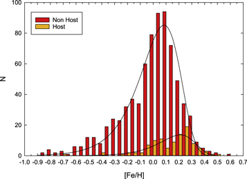
Figure 7. Histogram for [Fe/H] of "non-hosts" and hosts. The smooth curves are four-parameter Weibull fits. The peaks are offset by 0.12 dex, and a Mann–Whitney test indicates that the two distributions are different.
Download figure:
Standard image High-resolution imageThere are more than 20 physical pairs in this sample. After eliminating those with at least one member of the pair below 4500 K, or with a rotational velocity more than 20 km s−1, 19 pairs remain. The mean difference in [Fe/H] between the components is 0.083 dex, with the largest difference being 0.4 dex. The data for this pair—BD +4 701 A and B—are of lower quality than the bulk of the data. Eliminating this pair lowers the mean difference to +0.065, with a standard deviation of 0.062. This agreement is excellent and boosts confidence in the abundance analysis.
4.3. Li, C, and O in Dwarfs
4.3.1. Lithium
Lithium in dwarfs has three aspects that require at least a modest discussion. First is the depletion/dilution of lithium as a function of mass or temperature. Second, do any of the "non-dwarfs" exhibit high lithium abundances that could signal they are pre-main sequence stars? Lastly, a topic that undoubtedly will not be settled here: Do planet hosts show higher lithium abundances than non-hosts?
Figure 8 shows two representations of the astration of lithium—the top panel shows lithium versus effective temperature, and the bottom panel lithium versus mass. The stars shown in Figure 8 are only those stars that meet the dwarf criteria, but planet hosts are included. Moreover, the temperature range shown in Figure 8 is the complete sample range. Lithium abundances are not especially gravity-sensitive, and the abundances are derived using a detailed spectrum synthesis. Note that, at 4000 K, the solar lithium abundance of log εLi = 1.0 produces a feature with an equivalent width over 10 nm, making the abundances at lower temperatures relatively secure.
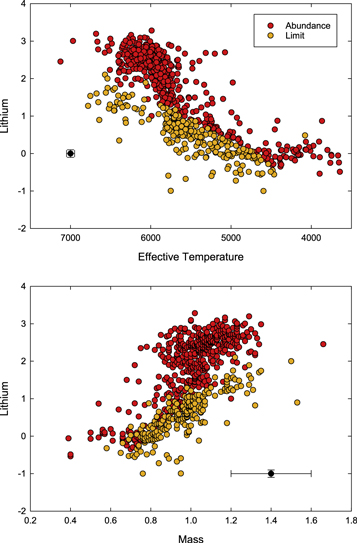
Figure 8. Top Panel: lithium abundance vs. effective temperature. Bottom Panel: lithium abundance vs. mass. Both show the dwarfs only. Astration as a function of temperature/mass is most pronounced in the data.
Download figure:
Standard image High-resolution imageThe strong decrease in lithium abundances as a function of decreasing mass and temperature, as seen in Figure 8. is not new—having been noted by Lambert & Reddy (2004), as well as Luck & Heiter (2007). What is new here is the number of stars—600+ here, versus 200+ in the previously cited works. Additionally, the data of Lambert & Reddy (2004) do not extend to the lower masses and temperatures of this study. The explanation for the growth of astration as mass declines is simple; convection depth increases as the mass declines, until, at some point, stars become totally convective. Deeper convection transports lithium to temperatures where it is destroyed, leading to the observed decline in surface abundance.
Two other features seen in Figure 8 are of note. The first is that the strongest decline in lithium abundance occurs rather abruptly at a mass of 0.8 MSun; or alternately, at about 5600 K in effective temperature. Second, by Teff ∼ 5000 K, and most definitely by 4500 K, the lithium abundances have dropped to a plateau value of about log εLi ∼ 0, which is about one-tenth solar. This "constant" abundance implies that the convection depths achieved in these stars is the same. Given the small range in mass—about 0.5 to 0.8 MSun—this is not especially surprising.
In Figure 9, the lithium abundances are once again plotted versus temperature. However, in this plot, the "non-dwarfs" are included. What is obvious is that the "non-dwarf" lithium abundances match up very well with the dwarf abundances. This match-up means the "non-dwarfs" are subgiants just coming off the main sequence. The only exception is the cool "non-dwarf" HD 98800. This star is an RS CVn variable with a spectral type of K5V(e). It is a young pre-main sequence star (Elliott et al. 2016 and references therein).
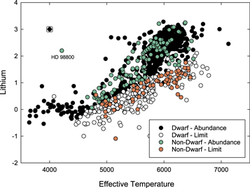
Figure 9. Lithium vs. temperature with both dwarfs and "non-dwarfs." The only non-dwarf that is a young star is HD 98800. The other non-dwarfs have lithium abundances consistent with the dwarfs and are subgiants.
Download figure:
Standard image High-resolution imageThe lithium abundance found in planet-hosts relative to non-hosts has been a subject of ongoing debate. The contention is that the stars hosting close-giant planets have higher lithium abundances than similar non-hosts. Evidence for this position has most recently been put forward by Gonzalez (2014, 2015). The counter-argument has been espoused by Luck & Heiter (2006) and Ghezzi et al. (2010). There are more than 100 planet-hosts in this work, all found by radial velocity variations, which means that they are mostly systems containing close-giant planets. The host systems have both dwarf and subgiant stars; in Figure 10, the lithium abundances of all non-hosts are shown overplotted with the lithium abundances of the host systems. The non-hosts are limited to rotational velocities less than 20 km s−1, and the temperature range is that spanned by the host stars. Given the sensitivity of lithium to effective temperature, the virtue of this work (regarding the lithium comparison) is the internal consistency of its temperature scale. Examination of Figure 10 indicates that there is no discernible difference in the lithium abundances of the planet- hosts and non-hosts.

Figure 10. Lithium vs. temperature with the planet-hosts segregated from the non-hosts. Both classes appear to have equivalent lithium abundances at the same temperature.
Download figure:
Standard image High-resolution imageTo further examine possible abundance differences between planet hosts and non-hosts, the lithium abundances excluding the limits have been binned in 100 K increments. The resulting average lithium abundance versus effective temperature data are shown in Figure 11. What is apparent is that, for the stars in this work, the hosts do not have lithium abundances above those of the non-hosts. In fact, except for two higher-temperature bins, the host lithium abundances are lower than those of the non-hosts. In all cases, the one-sigma error bars for the mean host and non-host lithium abundances overlap.

Figure 11. Mean lithium abundances for non-host and host dwarfs vs. effective temperature. The bin size is 100 K, and both the temperature and lithium abundance shown are the average value within the bin. The error bars on the lithium abundance are one standard deviation. Note that the host abundances tend to be lower than the corresponding non-host lithium abundance.
Download figure:
Standard image High-resolution imageIn Figure 12, histograms of host and non-host lithium abundances for three temperature bins are given. These are the three most-populated bins in the hosts, and include one of the two bins where the hosts have mean lithium abundances above the non-hosts. The second bin with high host abundance has only three host stars in it. Also shown for each bin is a Gaussian fit to the non-host data. For the two higher-temperature bins, including the bin that has a higher host mean—the 6000 to 6100 K bin—it appears that the host data distributes across the range of non-host data. A Mann–Whitney test indicates that the host and non-host abundances in the two high-temperature bins are not statistically different at P = 0.379 and 0.096 respectively. The lower temperature bin does show a statistical difference at P = 0.031, but the host abundance average is lower than the non-host is this bin.
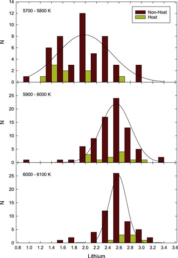
Figure 12. Histograms of the lithium abundances in three temperature bins. Astration effects are obvious in the abundances; the decline in mean abundance and the broadening of the Gaussian fit width going to lower temperature. A Mann–Whitney test indicates that only the lower temperature set shows a significant difference between the hosts and non-hosts. In that temperature range, the hosts show a lower abundance than do the non-hosts.
Download figure:
Standard image High-resolution imageThus, it appears that stars with planets have lithium abundances that are not enhanced relative to non-hosts. Although this result will not satisfy everyone, it is what this analysis supports.
4.3.2. C and O
The behavior of carbon and oxygen in the local region is well-determined—for a full discussion, see Nomoto et al. (2013) and/or Hinkel et al. (2014). The trends are that both [C/Fe] and [O/Fe] decrease with increasing [Fe/H]. These trends are a result of the increased importance of iron production in Type Ia supernovae as time proceeds. In Figure 13, these trends along with C/O versus [Fe/H] are shown for this sample of stars. The stars plotted have a minimum effective temperature of 4500 K. The data presented here are in accord with previous studies.

Figure 13. Top Panel: [C/Fe] vs. [Fe/H]. Middle Panel: [O/Fe] vs. [Fe/H], Bottom Panel: C/O vs. [Fe/H]. The effects of galactic chemical evolution dominate the data, with the influence of Type Ia supernovae increasing as solar [Fe/H] is approached. What is curious is that the C/O ratio at [Fe/H] of 0 is about 0.4 rather than the solar ratio of 0.55.
Download figure:
Standard image High-resolution image
In Figure 13, there are a few stars that appear to have [C/Fe], [O/Fe], or C/O ratios that differ considerably from the bulk of the data. For the [C/Fe] data (Figure 13, top panel), the stars that scatter above the bulk of the data have effective temperatures less than 5000 K, and the larger number of those cluster between 4500 and 4700 K. The better interpretation of the high [C/Fe] ratios in these stars is that the ratio is overestimated due to blends in the C2 lines. There are two stars—HD 210640 and HR 6469—with very low [C/Fe] ratios. These stars have Teff > 5500 K, and the lack of C i lines is pronounced. It appears that the low carbon content has not been previously noted. These stars are possibly related to the weak-G band stars (Palacios et al. 2016; Adamczak & Lambert 2013).
The [O/Fe] data (Figure 13—middle panel) show the usual increase in [O/Fe] with decreasing [Fe/H]. There is some scatter at above-solar [Fe/H] ratios toward low [O/Fe] ratios. The low oxygen abundances are likely due to underestimates of the oxygen strength, due to continuum placement or noise problems. The stars with low [O/Fe] ratios are predominately cooler than 5500 K, making the oxygen abundance depend on the weak [O i] line—and thus, susceptible to such problems.
Lastly, C/O versus [Fe/H] is shown in the bottom panel of Figure 13. The bulk of these stars have subsolar C/O ratios. At solar [Fe/H], the C/O ratio is about 0.4, whereas the solar ratio is 0.55. This offset is also seen in the dwarf study of Luck & Heiter (2006). What is curious is that the local giants show a mean C/O of about 0.4 at solar [Fe/H] (Luck 2015), although one would expect the giants due to CN-processing to have a lower C/O than the dwarfs. Where the problem lies, if there is one, is yet to be determined. Note that, as the [Fe/H] ratio falls, so does the C/O ratio; at [Fe/H] ∼ 0, the nominal C/O ratio is 0.4, whereas the ratio is about 0.2 at [Fe/H] ∼ −0.8.
5. CONCLUDING REMARKS
Although this study finds no spectacular new result, it does provide a large sample of self-consistently analyzed dwarfs and subgiants in the local vicinity. Accurate abundances demand accurate equivalent widths. The new method of equivalent width determination described here provides a significant enhancement in reliability of the input data for the investigation. The abundance analysis adds more substance to the abundance work that underpins out understanding of the local region.
One of the more significant problems this study cannot approach is the difficulty of determining reliable abundances in dwarfs cooler than 4500 K. One approach to this problem would be to use near-infrared spectra of cool bright dwarfs. Such spectra might also allow one to isolate the ionization problem using unblended Fe i and Fe ii lines. Serious current deficiencies that need rectification before such studies can be realized include more and better laboratory oscillator strengths and damping coefficients.
As the last point, some thought needs to be given to the central idea behind these studies: What is the standard of normalcy in the local region for abundances, and specifically, how does the Sun compare? The average star in the solar neighborhood has a composition like the average shown in Figure 4. An additional piece of information is located in Figure 11. Stars of the same temperature of the Sun most commonly have lithium abundances of about 1.8 dex. This study indicates that the Sun is somewhat atypical of its neighbors. The ways that it differs are:
- 1.The lanthanide abundances of the Sun are about 0.2 dex lower than those of its average neighbor.
- 2.The lithium abundance of the Sun is in the lower range of abundance compared to local stars of like temperature.
- 3.The C/O ratio of the Sun is high compared to its neighbors: 0.55 versus 0.4.
These differences are modest, but real. The second item above is the least problematic—lithium is very sensitive to convection depth and precise prior history. The C/O ratio and lanthanide abundance are primordial, and reflect the immediate supernovae history prior to the formation of the proto-solar nebula.
Financial support by Case Western Reserve University made possible the McDonald Observatory observations used in this work. Gregory Tobar-Gomez was instrumental in helping to develop the equivalent width pseudo-Voigt procedures. The Sandiford and HET echelle spectra used here are available through the FGK Spectral Library. Also available from the FGK Spectral Library are EXCEL format versions of all tabular material derived as part of this analysis. The ELODIE archive at Observatoire de Haute-Provence (OHP) also provided part of the spectroscopic data. The SIMBAD database, operated at CDS, Strasbourg, France and satellite sites, and NASA's Astrophysics Data System Bibliographic Services were instrumental in this work.