


Abstract
Large Sky Area Multi-Object Fiber Spectroscopic Telescope (LAMOST) low- and medium-resolution spectroscopic surveys are important for determination of the orbital parameters and chromospheric activity of extrasolar planet systems. We crossmatched the exoplanet catalog confirmed before 2021 March 11 with the LAMOST DR7 survey to study their properties. There are 1026 targets with exoplanets observed in the LAMOST DR7 low-resolution spectroscopic survey and 158 targets in the medium-resolution spectroscopic survey. We have calculated the equivalent width of the Hα line and determined their stellar activity. The Hα and flare intensities are almost constant for the Rossby number Ro ≤ 0.12 in the saturated regime and decrease with increasing Ro in the unsaturated regime. In addition, we searched the flare events of all stars with exoplanets in the Transiting Exoplanet Survey Satellite (TESS), Kepler, and K2 surveys. Among the 733 extrasolar planetary systems observed by TESS, we found 481 flares from 57 stars. For Kepler data, we obtained the light curve of 1699 stars and found 1886 flares from 417 stars. For K2 data, we obtained the light curves of 347 stars and found 467 flares from 89 stars. There were light curves of 361 objects with obvious eclipse observed from the TESS survey. We have fitted their light curves with a high signal-to-noise ratio using the JKTEBOP program, and we reobtained the orbital parameters, such as inclination, radius, and period. In the end, we made a judgment on the habitability of exoplanets of stars with flares.
Export citation and abstract BibTeX RIS

Original content from this work may be used under the terms of the Creative Commons Attribution 4.0 licence. Any further distribution of this work must maintain attribution to the author(s) and the title of the work, journal citation and DOI.
1. Introduction
Solar activities impact space weather plus the lives and actions of human beings, such as commercial aviation and communication (Lingam & Loeb 2017; Linsky 2019; Tu et al. 2020). Planets are where we live, and stars provide the necessary conditions and energy for our survival. Magnetic activities are relevant to the host star, planets, star−planet interactions, and so on. The studies of the activity and parameters of host stars and exoplanets are important to help us better find an alternate livable planet and explore extraterrestrial civilization. Robinson et al. (1990) determined chromospheric activity properties of 50 main-sequence K and M stars using Hα and Ca ii H and K lines. Eker et al. (1995) explored the details of the Hα profile of 25 chromospheric active binaries. Later, the magnetic activity of 53 G and K dwarf stars was documented through the He i D3 line (Saar et al. 1997). Furthermore, due to the Sloan Digital Sky Survey (SDSS; Stoughton et al. 2002; Abazajian et al. 2009) and LAMOST survey (Wang et al. 1996; Su & Cui 2004; Cui et al. 2012), the study of stellar chromosphere activity has reached a new stage. West et al. (2008) analyzed the spectra of more than 38,000 low-mass stars published as SDSS data and confirmed that the fraction of stellar magnetic activity decreases with the increase of the vertical distance from the Galactic plane. Cuntz et al. (2000) found stellar chromospheric activity enhancements possible owing to the interactions between extrasolar giant planets and their host stars. Shkolnik et al. (2003) first detected the synchronous enhancement in emission of Ca H and K lines in short-period planetary orbit in HD 179949. Later, they also monitored the chromospheric activity in Ca H and K lines, and some of them also exhibited short- and long-term chromospheric activity variation (Shkolnik et al. 2005, 2008). Zhang et al. (2016) detected 6391 active M stars from the 99,741 stars in the M-star catalog of the LAMOST survey using the Hα line. Zhang et al. (2021) used 738,477 LAMOST low-resolution spectra and 272,181 medium-resolution spectra to explore the chromospheric statistical properties and variations of M stars. The Balmer lines are important to study the chromospheric activity of stars with exoplanets.
Stellar magnetic activity like stellar flares, coronal mass ejections, and high-energy emission affect the exoplanetary atmosphere (Poppenhaeger 2015; Kay et al. 2016). Ip et al. (2004) used an MHD numerical code to simulate the possible scenarios of magnetospheric interaction of hot Jupiters with their host stars. For some of them with close-in extrasolar giant planets and semimajor axes less than 0.05 au, one might be able to generate a powerful solar-flare-like process. Stellar flares are frequent events on many active host stars with exoplanets, which impact the atmospheres of exoplanets. Chadney et al. (2017) developed a model to describe the upper atmosphere of extrasolar giant planets using stellar flares. Stellar magnetic activity was studied based on the light curve using space telescope data, such as the Kepler mission (Borucki et al. 2010), the TESS mission (Ricker et al. 2014), and so on. Walkowicz et al. (2011) searched 23,000 cold dwarfs in Kepler Quarter 1 data and found 373 stars with flare events. Balona (2012) integrated several thousand light curves of Kepler and found 19 A-type stars, 27 F-type stars, and 25 G-type flare stars. This was the first time that A-type flare stars were clearly observed. Armstrong et al. (2016) detected the superflares in the light curve of Kepler-438. Bentley et al. (2009) found a stellar flare occurring during a transit of the exoplanet OGLE-TR-10b with an active host star. They found 17 host stars of 284 flare stars that may deplete an Earth-like atmosphere by repeated flare events (Howard et al. 2019). Using the K2 data, the flaring events of TRAPPIST-1 continuously affect the atmospheres of the orbiting exoplanets, which probably makes them less favorable for harboring life. Günther et al. (2020) found 8695 flares of 673 M stars in the first 2 months of TESS and obtained their energy in the range 1031.0–1036.9 erg. They also found four flaring M-dwarf host exoplanet candidates and discussed how the flare affects exoplanet habitability. Tu et al. (2020) found that there are superflares in four stars accompanied by unconfirmed hot planet candidates, which might be caused by stellar activities instead of planet−star interactions. However, they did not find a significant excess fraction of flare stars with planet candidates, as compared with flare stars without planet candidates (Tu et al. 2021). As a considerable number of exoplanets have been found, it is necessary to do so.
The discovery of the PSR 1257 + 12 planets answered the question whether there are planets outside the solar system (Wolszczan & Frail 1992). Another exoplanet, 51 Peg b, discovered by radial velocity method in 1995, tells us that there are exoplanets around Sunlike stars (Mayor & Queloz 1995). These discoveries open a new chapter in planetary exploration. So far, more than 4400 exoplanets have been discovered. Charbonneau et al. (2000) and Henry et al. (2000) determined that there is an unknown celestial body near HD 209458 by radial velocity measurements. Then, they found the transiting process of unknown objects passing through HD 209458 through optical observation, and this is also the first detection of a transiting planet by the transiting method. Bakos et al. (2004) proposed the concept of the Hungarian Automated Telescope (HAT), a ground-based telescope for large-scale search of transiting planets. Haswell (2006) used WASP data to calculate the physical parameters of the first two exoplanets discovered by WASP. More than 200 exoplanets have been discovered in the above two projects. But the number of exoplanets is increasing after Kepler. As of 2021 March 27, more than 2800 exoplanets have been discovered in Kepler and K2. The TESS mission has also identified 120 exoplanets and found 2597 candidate planets. It is also important to revise the parameters of exoplanets, such as mass, orbital radius, eccentricity, and orbital inclination.
Currently, LAMOST DR7, TESS, Kepler, and K2 missions have released a substantial amount of data. A combined study of these data allows us to better obtain various parameters of exoplanets and their host stars and explore the habitability of exoplanets. In Section 2, we provide a brief introduction to the data we need to use. In Section 3, we use the spectral data of LAMOST DR7 to explore the magnetic activity of the host stars of the exoplanets. In Section 4, we describe the search for the flares of these stars, based on the photometric data acquired by TESS, Kepler, and K2. In Section 5, we fit the light curve and solve the parameters of exoplanets and their host stars, and we make a preliminary judgment on the habitability of exoplanets by using the flare data.
2. LAMOST Spectra and TESS Light Curve
2.1. LAMOST Spectra
LAMOST is a special reflecting Schmidt telescope lying in the north–south direction. It has a wide field of view of 5° (Cui et al. 2012; Deng et al. 2012; Luo et al. 2012, 2015). Because the shape of the reflecting Schmidt plate of the telescope was changed with each different decl. delta of the objects and in the tracking observation, its effective aperture is in the range of 3.6–4.9 m (Wang et al. 1996; Cui et al. 2012). As it has a diameter of 4 m, celestial bodies as dark as 20.5 magnitude can be observed within 1.5 hr of exposure. And because it has a field of view of up to 5°, 4000 optical fibers can be placed in the focal plane to transmit the light of remote objects to multiple spectrometers and obtain their spectra simultaneously. We can obtain several stellar parameters from the spectral data, such as effective temperature (Teff), surface gravity (log g), and metallicity ([Fe/H]). Based on the release of LAMOST DR7 (2019 June 8), LAMOST has released 10,608,416 low-resolution (R ∼ 1800) spectra and 3,889,383 medium-resolution (R ∼ 7500) spectra. 7 We crossmatched the LAMOST spectral survey with the exoplanet catalog published before 2021 March 11. The results are listed in Table 1. A total of 1928 spectra from 1026 stars meeting the requirements were found in the LAMOST low-resolution spectral survey, and 282 spectra from 121 stars were found in the LAMOST medium-resolution survey. We selected the spectra with signal-to-noise ratio (S/N) > 10 as our sample. Finally, 1669 low-resolution spectra of 940 stars and 282 medium-resolution spectra of 121 stars were obtained, and the distributions of the spectral types are shown in Figure 1.
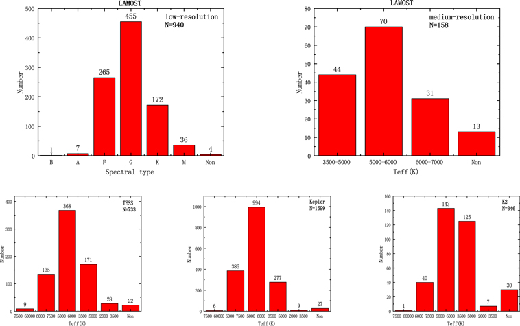
Figure 1. Stellar spectral types and effective temperature distributions of our objects in the different surveys.
Download figure:
Standard image High-resolution imageTable 1. Observation Targets
| Property | Number |
|---|---|
| TESS observations | 733 |
| Kepler observations | 1697 |
| K2 observations | 347 |
| LAMOST DR7 low-resolution observations | 940 |
| LAMOST DR7 medium-resolution observations | 121 |
| LAMOST DR7 low-resolution active observations | 721 |
| LAMOST DR7 medium-resolution active observations | 82 |
Download table as: ASCIITypeset image
We can study stellar activity using many chromospheric activity lines, such as Hα, Hβ, Hγ, Hδ, Ca ii, and Mg ii IRT lines (Long et al. 2018). The LAMOST low-resolution spectra include all the optical chromospheric activity indicators, and we usually use Hα equivalent width (EW) to judge the activity. The wavelength ranges of LAMOST medium-resolution spectra include 4950−5350 Å and 6300−6800 Å. The wavelength of the Hα line is 6562.8 Å, and therefore we can also study chromospheric activity from the medium-resolution spectra. In this work, we used both low-resolution (R = 1800) spectra and medium-resolution (R = 7500) spectra to calculate the EW of the chromospheric activity lines and make a judgment on the stellar activity of the host star of the exoplanet.
2.2. TESS Light Curve
TESS is a space telescope that was launched from the Cape Canaveral Air Force Base in the United States on 2018 April 18. The mission of TESS is the exploration of extraterrestrial planets for a full-sky survey. TESS is used to observe 26 sectors within the 24° × 96° field of view, each sector lasting 27 days, for a total of 2 yr of observation. Its observation sensitivity is sufficient to discover terrestrial rocky planets and gas giant planets in various possible orbits, which ground-based telescopes cannot do. Its main goal is to find planets that are closer to stars with magnitude less than 13 (Kossakowski et al. 2019). We revised the size and period of the planet by the light curve of the TESS survey. It will conduct photometry of more than 200,000 stars during a 2 yr mission with a cadence of approximately 2 minutes. The expected goal is to find about 1250 new exoplanets with occultation (Barclay et al. 2018). Of course, we can also use the light curve provided by the TESS telescope to find the stellar flare events and calculate the flare energy, flare time, and so on. This work used the Lightkurve package (Cardoso et al. 2018) in Python to process the light curve. By crossmatching the exoplanet catalog with the first 31 sections of TESS, we obtained 1575 light curves of 733 targets of stars with exoplanets. Since these stars can only obtain a few spectral types from LAMOST data, we have made statistics on the distribution of these stars according to the effective temperature, as shown in Figure 1.
2.3. Kepler and K2 Light Curve
The Kepler mission started on 2009 May 2 and ended on 2013 May 11, and the telescope was launched in an elliptical orbit around Earth. It points to the sky in the direction of Cygnus and is used to observe light curves of nearly 200,000 stars to search transit signals. It uses use these photometric signals to find exoplanets and determine the universality of the existence of exoplanets in the Milky Way. The light-curve files are divided into two kinds: 30-minute exposures and 1-minute exposures. At the same time, we can also use these data to study the variability in the brightness of stars or binary stars. Because the telescope lost its second reaction wheel in 2011, the Kepler mission ended and the K2 mission began. The K2 mission started on 2014 February 4 and ended on 2018 September 26. It observed 100 deg2 of sky at 20 different observation points along the ecliptic, and the observation time of each point was 80 days (Ricker et al. 2014). The K2 mission can also generate the same light-curve data file as the Kepler mission. We also use the Lightkurve package (Cardoso et al. 2018) to process and extract these curves. Thus, the Kepler and K2 missions have identified 2394 and 426 exoplanets, respectively, and there are more than 3000 extraterrestrial candidates waiting to be confirmed. In this work, we primarily use the data provided by Kepler and K2 in order to search for the flares and calculate the flare energy. We found 1886 flares from the light curves of 1699 stars from the Kepler mission. These 1886 flares come from 417 host stars. Based on 347 extrasolar planet targets of K2, we found 467 flares from 89 stars and calculated the energies of the flares. The effective temperature distribution of stars in Kepler and K2 samples is also shown in Figure 1. The positions of our targets of the LAMOST, TESS, Kepler, and K2 missions involved in this work are shown in Figure 2, where the blue circles represent all discovered exoplanets and other colored circles represent the observational distribution of each mission.

Figure 2. Blue circles represent all identified exoplanets, and red and green circles represent the distribution of exoplanets that can be observed by various telescopes. Left panel: LAMOST field; middle panel: TESS field; right panel: Kepler and K2 fields.
Download figure:
Standard image High-resolution image3. Chromospheric Activity
3.1. Equivalent Widths of Chromospheric Activity Lines
We used the LAMOST low-resolution and medium-resolution spectral data with S/N > 10 and calculated their EW of the Hα emission lines for all spectra. For the medium-resolution spectra, we first normalized the spectral data. There are a lot of cosmic rays for single spectra. First, we removed the cosmic rays from all the medium-resolution spectra. When the flux data are greater than three times the standard deviation, they are regarded as abnormal data. We then replaced the outlier with the average flux of the four adjacent points. We did not consider the wavelengths between 6550 and 6580 Å in the cosmic-ray processing in order to avoid removing the Hα emission line. Then, we used the processed spectrum to calculate the EW of the Hα line. First, Gaussian fitting is performed on the normalized spectral image to determine the central position of the Hα emission line, and then the width of 4 Å on both sides is integrated to obtain the EW of the Hα line. At the same time, we also estimate the error of the EWs. We used Monte Carlo simulation to estimate the error of EW. The random flux values are generated by Gaussian distribution, and the random flux values of all data points are combined to form a simulated spectrum. Then, we generate 100 simulated spectra, calculate the Hα EW of the 100 simulated spectra, and finally use the standard deviation of the 100 EWs as the final error. For both low- and medium-resolution LAMOST spectra, we collected the Teff, log g, [Fe/H], and other parameters obtained by LAMOST. The parameters associated with the low-resolution spectral data are listed in Table 2, and the parameters of LAMOST medium-resolution spectra are listed in Table 3.
Table 2. Low-resolution Spectral Parameters of Exoplanet Host Stars in LAMOST DR7
| LAMOST Name | HJD | EXP | SN | Sp | RV | EW Hα | SN Hα | Height | Fe/H | Logg | Teff |

|
|---|---|---|---|---|---|---|---|---|---|---|---|---|
| (1) | (2) | (3) | (4) | (5) | (6) | (7) | (8) | (9) | (10) | (11) | (12) | (13) |
| J105509.35-004413.8 | 56,671.15556 | 1800 | 151.64 | G6 | 64.93 ± 4.42 | −1.27004 | 55.69876 | 10.01455 | −1.322 ± 0.104 | 3.516 ± 0.176 | 5252 ± 108 | 1.330E−05 |
| J195704.32+451338.7 | 57,283.84444 | 4500 | 25.99 | K5 | -102.85 ± 5.33 | −0.23666 | 19.85962 | 8.88513 | −1.267 ± 0.305 | 4.462 ± 0.514 | 4276 ± 320 | 9.660E−06 |
| J191447.67+394229.8 | 56,094.04583 | 1600 | 31.18 | G4 | 15.39 ± 11.88 | −1.19468 | 30.16848 | 3.62221 | −0.816 ± 0.194 | 4.107 ± 0.329 | 5584 ± 204 | 6.440E−05 |
| J191025.11+421000.4 | 56,432.09514 | 3000 | 143.28 | G2 | -5.47 ± 4.58 | −1.258 | 60.00805 | 9.9442 | −0.502 ± 0.014 | 4.227 ± 0.025 | 5836 ± 15 | 9.840E−05 |
| J194755.44+431235.1 | 57,303.825 | 1800 | 90.53 | G3 | −89.28 ± 5.34 | −1.31078 | 60.59665 | 15.25145 | −0.516 ± 0.207 | 4.258 ± 0.347 | 5562 ± 223 | 4.870E−05 |
| J195323.59+472928.4 | 57,283.84444 | 4500 | 92.94 | G7 | -59.47 ± 5.29 | −0.78481 | 63.54518 | 7.25844 | −0.511 ± 0.038 | 4.336 ± 0.066 | 5358 ± 40 | 7.730E−05 |
| J005930.25+041340.2 | 56,199.04549 | 1200 | 50.27 | F2 | −30.57 ± 13.66 | −0.81033 | 57.60905 | 6.61819 | −0.506 ± 0.061 | 4.214 ± 0.105 | 6066 ± 64 | 2.265E−04 |
| J005930.25+041340.0 | 58,491.77083 | 1800 | 418.38 | G3 | −20.3 ± 4.46 | −1.39338 | 75.49181 | 15.05395 | −0.506 ± 0.061 | 4.214 ± 0.105 | 6066 ± 64 | 1.355E−04 |
| J190645.48+391242.9 | 56,811.125 | 1800 | 160.35 | F2 | −42.87 ± 5.46 | −1.69109 | 59.67443 | 14.49667 | −0.336 ± 0.021 | 4.296 ± 0.037 | 6081 ± 22 | 9.120E−05 |
| J135733.43+432936.5 | 57,527.96597 | 1800 | 142.79 | K5 | −48.15 ± 4.1 | −0.67577 | 84.68954 | 14.49785 | −0.336 ± 0.054 | 4.558 ± 0.092 | 4397 ± 56 | −2.990E−06 |
| J194401.69+445112.4 | 56,913.85972 | 1800 | 379.16 | G2 | −69.42 ± 4.54 | −1.43763 | 57.3346 | 12.79337 | −0.333 ± 0.013 | 4.012 ± 0.025 | 5737 ± 16 | 6.110E−05 |
| J194717.49+480627.2 | 56,549.87292 | 1800 | 73.35 | K3 | −114.210 ± 3.77 | −0.84604 | 61.67999 | 12.74477 | −0.331 ± 0.04 | 4.528 ± 0.068 | 4633 ± 41 | −1.630E−06 |
Note. Column (1): LAMOST name. Column (2): observation time. Column (3): local modified Julian minute. Column (4): signal-to-noise ratio. Column (5): spectra type. Column (6): radial velocity. Columns (7)–(9): EW of the Hα line, error, and height. Column (10): metallicity from LAMOST. Column (11): surface gravity from LAMOST. Column (12): effective temperature from LAMOST. Column (13): LHα /Lbol.
Only a portion of this table is shown here to demonstrate its form and content. A machine-readable version of the full table is available.
Download table as: DataTypeset image
Table 3. Medium-resolution Spectral Parameters of Exoplanet Host Stars in LAMOST DR7
| LAMOST Name | SN | RV | EW Hα | EW Hα err | Teff | Logg | Fe/H |

|
|---|---|---|---|---|---|---|---|---|
| (1) | (2) | (3) | (4) | (5) | (6) | (7) | (8) | 9 |
| J005114.31 + 065047.2 | 75.55 | −5.69 ± 0.83 | −1.3957 | 0.0240 | 5639 | 4.314 ± 0.033 | 0.059 ± 0.021 | 5.228E−05 |
| J112829.26 + 014126.2 | 108.34 | 2.87 ± 0.54 | −1.3556 | 0.0259 | 5549 | 4.622 ± 0.047 | −0.017 ± 0.029 | 4.269E−05 |
| J082744.79 + 173445.5 | 144.46 | 29.41 ± 0.45 | −0.5085 | 0.0320 | 4481 | 4.609 ± 0.048 | −0.153 ± 0.029 | 8.142E−06 |
| J085117.48 + 114522.6 | 437.68 | 29.9 ± 0.8 | −0.8557 | 0.0509 | 4316 | 2.126 ± 0.861 | −0.025 ± 0.535 | −1.124E−05 |
| J034055.09 + 204409.9 | 70.11 | 15.08 ± 0.77 | −1.4491 | 0.0380 | 5764 | 3.724 ± 0.072 | 0.094 ± 0.043 | 6.914E−05 |
| J034314.22 + 163804.3 | 35.48 | 3.07 ± 1.72 | −1.0428 | 0.0399 | 5298 | 4.561 ± 0.051 | 0.248 ± 0.031 | 4.252E−05 |
| J185753.32 + 395442.5 | 168.08 | −44.01 ± 0.41 | −1.4868 | 0.0193 | 5693 | 4.293 ± 0.072 | 0.104 ± 0.048 | 5.103E−05 |
| J190254.83 + 423916.3 | 58.86 | −12.9 ± 0.99 | −1.2563 | 0.0216 | 5600 | 4.16 ± 0.049 | −0.02 ± 0.03 | 6.454E−05 |
| J042152.70 + 574901.8 | 201.78 | −15.44 ± 0.3 | −1.7830 | 0.0400 | 6987 | 4.123 ± 0.027 | −0.106 ± 0.017 | 3.150E−04 |
| J042456.72 + 184938.6 | 33.71 | 11.25 ± 1.89 | −1.2693 | 0.0354 | 5597 | 3.914 ± 0.073 | 0.201 ± 0.043 | 6.254E−05 |
| J042941.56 + 263258.2 | 43.57 | 8.79 ± 5.78 | 17.5574 | 0.4428 | 4309 | 3.9 ± 0.105 | −1.821 ± 0.065 | 6.407E−04 |
| J043310.02 + 243343.2 | 171.3 | 10.01 ± 1.13 | 1.6163 | 0.0242 | 4127 | 4.143 ± 0.053 | −0.47 ± 0.034 | 5.556E−05 |
Note. Column (1): LAMOST name. Column (2): signal-to-noise ratio. Column (3): radial velocity. Columns (4)–(5): EW of the Hα line and error. Column (6): effective temperature. Column (7): surface gravity. Column (8): metallicity. Column (9): LHα /Lbol.
Only a portion of this table is shown here to demonstrate its form and content. A machine-readable version of the full table is available.
Download table as: DataTypeset image
3.2. Chromospheric Activity and Variation
To determine the chromospheric activity, we used the relationship between the EW of Hα and Teff to evaluate the activity of stars. In the project of determining the activity standard, we used several groups of data, which include the activity judgment line formulated by Fang et al. (2016, 2020) based on LAMOST low-resolution spectra, the catalog of standard stars published by Du et al. (2019) based on the LAMOST survey, and the standard stars obtained from the website 8 to jointly formulate a curve to evaluate the star activity of LAMOST medium-resolution spectrum. Zhao et al. (2015) have developed a curve to judge stellar activity by using the relationship between SHK and Teff. Our standard line also referred to his method in the final determination. Finally, we got a standard line similar to Fang et al. (2016, 2020), and this line is also suitable for LAMOST medium-resolution observations, so we continue to use their results. We plotted the results in Figure 3, where the red line is the activity judgment line formulated by the standard stars, the stars above this line are active, and the stars below this line are inactive. Using this method, we obtained 721 active stars among 940 samples with the LAMOST low-resolution spectra and 82 active stars from 121 samples with LAMOST medium-resolution spectra. We plotted the six samples with Hα obvious emissions from the LAMOST low-resolution spectra, as shown in Figure 4, and four samples with obvious Hα emission from the LAMOST medium-resolution survey, as shown in Figure 5.

Figure 3. Relationship of the EWs of Hα and stellar effective temperature, where the left panel shows LAMOST low-resolution spectra and the right panel shows LAMOST middle-resolution spectra. The red line is the activity judgment line formulated by the standard stars, the stars above this line are active, and the stars below this line are inactive.
Download figure:
Standard image High-resolution image
Figure 4. Spectra of the six examples showing the Hα emission line from the LAMOST low-resolution survey. Each panel contains the original spectrum (upper) and the normalized version (lower).
Download figure:
Standard image High-resolution image
Figure 5. Spectra of four examples showing the Hα emission line from the LAMOST medium-resolution survey. Each panel contains the original spectrum (upper) and the normalized version (lower).
Download figure:
Standard image High-resolution image3.3. Chromospheric Activity Level, 

In addition, we also calculated another physical quantity,  , of chromosphere activity. This value is the ratio of Hα luminosity to the bolometric luminosity (LHα
/Lbol), which is widely used as an index to judge the activity level of chromosphere activity (Hawley et al. 1996; Douglas et al. 2014; Frasca et al. 2016). We used a distance-independent method proposed by Walkowicz et al. (2004) to calculate LHα
/Lbol:
, of chromosphere activity. This value is the ratio of Hα luminosity to the bolometric luminosity (LHα
/Lbol), which is widely used as an index to judge the activity level of chromosphere activity (Hawley et al. 1996; Douglas et al. 2014; Frasca et al. 2016). We used a distance-independent method proposed by Walkowicz et al. (2004) to calculate LHα
/Lbol:
where χHα = FHα /Fbol. FHα is the flux of the continuum in the Hα line, and Fbol is the bolometric flux. EWbasal is the value of the red line in Figure 3. In this work, we used the method of Frasca et al. (2016) to estimate the value of χHα :

where σ is the Stefan−Boltzmann constant. We also listed all the  results in Tables 2 and 3.
It is well known that the rotation period is also closely related to stellar activity (Skumanich 1972), so we also studied the relationship between the activity of exoplanet host stars and their rotation period. First, we calculate the rotation period (P) of these samples by the Lomb−Scargle (Lomb 1976; Scargle 1982) method. Then, the Rossby number (Ro = P/τ) is calculated by using the method from Wright et al. (2011), where τ is the convective turnover timescale. We have plotted the relationship between  and Ro in Figure 6. We also discuss the relationship of activity and rotation in the two different states of saturated and unsaturated. The Ro value of the turnoff point is about 0.12. The Hα of the exoplanet system is almost constant for Ro ≤0.12 in the saturated regime. The Hα activity decreases with increasing Ro, and the slope of a power-law function is about 0.56 in the unsaturated regime. Our results are consistent with the previous results (Douglas et al. 2014; Fang et al. 2018).

Figure 6. (a) The relationship between  and Ro. (b) The relationship between the ratio of flare energy to luminosity and Ro. (c) The relationship between the flare amplitude and EWs of Hα. (d) The relationship between the ratio of flare energy to stellar luminosity and EWs of Hα.
Download figure:
Standard image High-resolution image4. Flare Detection
4.1. TESS Flare Measurements
We can search the flare events from the light curves obtained by the space telescope. The flare feature is a rapid rise and a slow decline process. There are many methods of searching for flare events (Gao et al. 2016; Shporer et al. 2016; Liakos 2017; Yang et al. 2017; Lin et al. 2019). We used a method similar to that of Wu et al. (2015).
First of all, we normalized the flux using the following formula:

where Fnorm is the normalized flux, FPDC is the pre-search data conditioning (PDC) flux, and Fmed is the median of the PDC flux. After obtaining the normalized light curve, we use polynomial fitting as the background light variation of the stars. We segment the light curve of different data sets. Through experiments, we give the best segmentation results. TESS data are segmented according to 1 day. The 30-minute exposure data of Kepler and K2 are segmented according to 5 days, and the 1-minute exposure data are segmented according to 1 day. Before fitting the light curve, we will subtract the average value of its time series from the abscissa to make its coordinates close to 0. And for the segmented light curve, each segment of the light curve has 60% of the overlapping part. This can avoid the Runge phenomenon caused by polynomial fitting. Taking all the TESS data as an example, the first segment of the light curve is 0−0.7 days, the second segment is 0.4−1.4 days, the third segment is 1.1−2.1 days, the fourth segment is 1.8−2.8 days, and so on. Taking 0.4−1.4 days of the second segment as an example, the first 30% of the second segment is the last part of the first segment, and the last 30% of the second part is the front part of the third segment. After performing these tasks, we begin to fit the segmented light curve. In order to find the polynomial of the most appropriate level, we will calculate the residuals after each fitting. When the residual is no longer significantly reduced, we considered that as the most appropriate fitting function. In order to avoid the mistake flare as the background during fitting, we eliminate the data points with three times above standard deviations and fit them again to obtain a new residual and a new fitting function. We repeat the process 10 times to obtain the most suitable fitting as the background of the light curve. Then, the fitting results are subtracted from the original light curve and the points greater than 4 times the standard deviation, which are regarded as the candidates of flares. Finally, from these candidates, if the points meet the characteristics of a flare event, that is, the light curve rises rapidly followed by a relatively slow decline, we consider it as a flare event. In the end, we visually inspected the detecting results to make our results more accurate and avoid other sources of contamination such as foreground asteroids or source confusion. We also deleted targets with neighboring stars within 4''. Figures 7, 8, and 9 show examples of flares from the TESS, Kepler, and K2 surveys, respectively. We have used the following two criteria to judge the start time and end time of flares: (1) During the process of the brightness increasing, we set the time when the brightness is higher than 5% of the peak value as the start time. (2) In the process of brightness decreasing, we set the time when the brightness is lower than 5% of the peak value as the end time (Lu 2019). The peak time is the moment when the brightness is strongest.

Figure 7. These are two examples of TESS flare search results. The left panels show a standard flare model, and the right panels show a flare search result with eclipse interference and a slight jitter of the light curve.
Download figure:
Standard image High-resolution image
Figure 8. These are two examples of Kepler flare search results. The picture on the left is an example of 1-minute data with missing data, and the picture on the right is an example of 30-minute data.
Download figure:
Standard image High-resolution image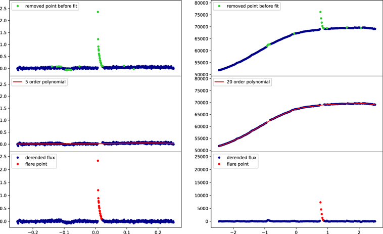
Figure 9. These are two examples of K2 flare search results. The left panels are an example of 1-minute data, and the right panels are an example of 30-minute data.
Download figure:
Standard image High-resolution imageAfter we run the program, there will be some misjudgment due to the following reasons: (1) misjudgment caused by discontinuity of the light curve, (2) misjudgment caused by changes in the light curve due to the transit of some eclipse binary or exoplanets (Shibayama et al. 2013b), and (3) the light change caused by the microlensing is also judged as a flare. Because the above misjudgment will be generated by using the program to search for the flare, human-eye screening is required at the end. Because our samples are stars with exoplanets, there are a large number of eclipses seen in the results of the flare. After we checked the flare events by eye, we eliminated about 25% of the results. In order to verify the correctness of the program, our group also tested other samples, and the results showed that there was only about 20% misjudgment.
4.2. TESS Flare Energies
We have found 481 flares from 57 stars using the TESS data. The energy of the flare was calculated by the following formula:

where Eflare is the flare energy, L* is the stellar luminosity, and Fflare is the normalized PDC flux. For the calculation of L*, we can use the following formula:

where R* is the stellar radius, σSB is the Stefan−Boltzmann constant, and T* is the effective temperature of the star. The radii are obtained from the Kepler or Gaia DR2 surveys (Huber et al. 2014; Gaia Collaboration et al. 2018). The effective temperatures were first obtained from LAMOST surveys (Luo et al. 2015). If there are no published temperatures of objects from the LAMOST survey, we used the temperature from the Kepler or Gaia survey (Huber et al. 2014; Gaia Collaboration et al. 2018). In this way, we can figure out their energies as soon as possible. The flare parameters are listed in Table 4. The flare energies of our samples are between 4.25 × 1030 erg and 3.23 × 1036 erg. Previously, Günther et al. (2020) searched the data of TESS in the first 2 months, and the energy range was 1031.0−1036.9 erg. Our range is almost consistent with the previous result (Günther et al. 2020). And the maximum values of flare energy obtained by Tu et al. (2020, 2021) with TESS data in 1 and 2 yr are 1.24 × 1036 erg and 1.77 × 1037 erg, respectively. The maximum flare energy we have obtained is similar to the previous results (Tu et al. 2020, 2021).
Table 4. Flare Parameters of Exoplanet System of TESS
| TESS ID | Peak Time | Begin | End | Duration | Amplitude | Teff | Radius | Energy |
|---|---|---|---|---|---|---|---|---|
| (1) | (2) | (3) | (4) | (5) | (6) | (7) | (8) | (9) |
| 388857263 | 1626.844890 | 1626.810862 | 1626.945584 | 0.134722 | 0.022645 | 3296 | 0.140 | 8.12E+31 |
| 439403362 | 1403.001683 | 1402.967656 | 1403.069043 | 0.101387 | 0.043685 | 3297 | 0.170 | 9.36E+31 |
| 388857263 | 1636.406625 | 1636.399681 | 1636.449680 | 0.049999 | 0.008756 | 3296 | 0.140 | 9.82E+31 |
| 388857263 | 1623.276848 | 1623.103931 | 1623.308098 | 0.204167 | 0.025264 | 3296 | 0.140 | 1.02E+32 |
| 439403362 | 1388.657287 | 1388.638537 | 1388.710760 | 0.072223 | 0.019165 | 3297 | 0.170 | 1.07E+32 |
| 98796342 | 1429.594312 | 1429.579729 | 1429.618618 | 0.038888 | 0.041033 | 3504 | 0.385 | 7.27E+32 |
| 307210830 | 1605.286485 | 1605.270513 | 1605.335790 | 0.065277 | 0.026030 | 3786 | 0.313 | 7.53E+32 |
| 419015728 | 1404.735331 | 1404.706512 | 1404.770401 | 0.063888 | 0.000325 | 5375 | 0.753 | 7.73E+32 |
| 441420236 | 2047.631539 | 2047.587094 | 2047.688485 | 0.101391 | 0.004062 | 3992 | 0.698 | 7.87E+32 |
| 206548902 | 1380.152836 | 1380.135128 | 1380.186516 | 0.051388 | 0.004021 | 3910 | 0.465 | 8.02E+32 |
| 260351540 | 2102.959559 | 2102.942198 | 2102.996365 | 0.054168 | 0.010216 | 5069 | 1.019 | 1.91E+34 |
| 410214986 | 2062.464485 | 2062.416569 | 2062.511013 | 0.094445 | 0.003446 | 5598 | 0.952 | 1.95E+34 |
| 410214984 | 2062.462402 | 2062.429069 | 2062.494347 | 0.065278 | 0.008182 | 4779 | 0.848 | 2.11E+34 |
| 88138162 | 1946.744675 | 1946.725926 | 1946.864813 | 0.138887 | 0.051850 | 3965 | 0.563 | 2.33E+34 |
| 410214986 | 1329.040514 | 1329.021070 | 1329.069681 | 0.048611 | 0.004344 | 5598 | 1.193 | 2.35E+34 |
| 260351540 | 2046.686902 | 2046.601486 | 2046.734819 | 0.133333 | 0.006895 | 5069 | 1.019 | 2.37E+34 |
Note. Column (1): TESS ID. Column (2): peak time. Column (3): start time. Column (4): end time. Column (5): flare duration. Column (6): flare height. Column (7): effective temperature. Column (8): stellar radius. Column (9): flare energy.
Only a portion of this table is shown here to demonstrate its form and content. A machine-readable version of the full table is available.
Download table as: DataTypeset image
4.3. TESS Flare Frequency Distribution
We use the maximum likelihood estimation method to calculate and estimate the flare frequency distribution (Goldstein et al. 2004; Bauke 2007; Li 2014; Newman 2005):

where n is the number of flares and Emax and Emin are the maximum and minimum values in the flare samples, respectively. For the calculation of error, we use the following formula:

In order to calculate the flare frequency distribution of all flare samples, we also calculate the flare frequency distribution of stars according to different effective temperature segments in Figure 10. Because the flare energy distribution obeys the power-law distribution only when the energy is higher (Newman 2005), the selection of energy range for calculating the power law will affect the results. Some power laws are calculated in the range above 1032 erg (Yang et al. 2017), some are 1034−1036 erg (Wu et al. 2015), some are 1031−1036 erg (Maehara et al. 2012; Shibayama et al. 2013a), and so on. Because the numbers of flare events in lower and higher energies are very limited, there is no statistical meaning. Therefore, we only fit the middle region. In the power-law calculation of all flares, we uniformly select flares with energy above 1033 erg. For the flare divided according to the effective temperature, we select the energy range for calculation according to the actual situation. For example, the flare energy of 2000–3500 K TESS data is low, which can be compared with that of M stars. we calculate its power law from 1031 erg. For Kepler 30-minute data, it also has a temperature range of 2000–3500 K. However, due to its long exposure time, it is difficult to find a flare below 1031 or 1032, so we start from 1032 erg.

Figure 10. Flare-frequency distributions of TESS, Kepler 1 minute, Kepler 30 minutes, and K2, where different colors represents different stellar temperature regions.
Download figure:
Standard image High-resolution imageFor all flares found by TESS, we get α = 1.86 ± 0.05, The α obtained from the flare results of 2000–3500 K, 3500–5000 K, and 5000–5000 K are 1.90 ± 0.11, 1.98 ± 0.11, and 1.96 ±0.08, respectively. Tu et al. (2020, 2021) got α = 2.16 ± 0.10 and α = 1.76 ± 0.11 from the 1 and 2 yr observational data of TESS, respectively. Our results confirmed the previous results (Tu et al. 2020, 2021).
4.4. Kepler and K2 Flare
We did the same work for Kepler and K2 data as for TESS, which are listed in Tables 5 and 6, respectively. For Kepler 30-minute data the energy range is 1.28 × 1032 erg to 8.16 ×1035 erg, and for 1-minute data it is 1.38 × 1031 erg to 1.82 ×1036 erg. Lin et al. (2019) obtained that the saturation energies of M, K, and G dwarfs are 1 × 1035 erg, 4 × 1035 erg, and 1 × 1036 erg, respectively. In the results of our Kepler data, the highest energy in the 2000–3500 K group is 1.66 × 1034 erg, in 3500–5000 K is 2.94 × 1035 erg, and in 5000–6000 K is 4.74 × 1035 erg. For 30-minute data, the power indices of all, 2000–3500 K, 3500–5000 K, 5000–6000 K, and 6000–7000 K are 1.81 ± 0.03, 2.00 ± 0.08, 2.02 ± 0.08, 1.78 ± 0.04, and 1.91 ± 0.13, respectively. For 1-minute data, the power index of all, 3500–5000 K, 5000–6000 K, and 6000–7000 K are 2.05 ± 0.03, 1.79 ± 0.06, 1.70 ± 0.03, and 1.90 ± 0.06, respectively. Due to the small number of flares found in K2 data, we combined the two data of K2 and made statistics, and the energy range is 2.48 × 1031 erg to 1.40 × 1039 erg. In the K2 results, there were several cases of extremely high flare energy. The flare energy of stars reached 1039 erg. After comparison with the data, we found that the radius of these stars was abnormally large. For example, the flare with energy of 1.40 × 1039 erg came from EPIC 203640875, and its radius reached 78.652 times the solar radius, resulting in its energy being 3 orders of magnitude higher than that of stars with similar solar radius. At the same time, there are many stars about 10 times the solar radius in our K2 sample, which leads to more high-energy flares in the data set. This also leads to a lower value of α in these effective temperature groups with these stellar flares. For all K2 data, α = 1.70 ± 0.04. α of 3500–5000 K, 5000–6000 K, and 6000–7000 K are 1.66 ±0.06, 1.83 ± 0.07, and 2.26 ± 0.16, respectively. The power-law indices of M, K, and G stars obtained by Lin et al. (2019) are 1.82 ± 0.02, 1.86 ± 0.02, and 2.01 ± 0.03, respectively. The data set of Shibayama et al. (2013a) shows that the power-law index of G-type stars is 2.2. Lu (2019) obtained the flare power-law index of M stars as 2.02 ± 11 by 17,432 flares. These results are consistent with each other.
Table 5. Flare Parameters of Kepler
| Object | Peak Time | Begin | End | Duration | Amplitude | Teff | Radius | Energy |
|---|---|---|---|---|---|---|---|---|
| (1) | (2) | (3) | (4) | (5) | (6) | (7) | (8) | (9) |
| KIC 2302548 | 973.895433 | 973.892197 | 973.901733 | 0.009535 | 0.021833 | 5095 | 0.780 | 1.16E+34 |
| KIC 2302548 | 973.895433 | 973.892197 | 973.935788 | 0.043591 | 0.021799 | 5095 | 0.780 | 1.15E+34 |
| KIC 2441495 | 300.354059 | 300.348270 | 300.376876 | 0.028606 | 0.020152 | 5207 | 0.795 | 8.53E+33 |
| KIC 2571238 | 300.354015 | 300.336647 | 300.365253 | 0.028606 | 0.007612 | 5546 | 0.810 | 3.96E+33 |
| KIC 2571238 | 900.443459 | 900.420300 | 900.457082 | 0.036782 | 0.006729 | 5546 | 0.810 | 2.98E+33 |
| KIC 3544595 | 1323.114570 | 1323.067062 | 1323.118827 | 0.051765 | 0.002288 | 5648 | 0.894 | 1.11E+33 |
| KIC 3544595 | 1337.504371 | 1337.500625 | 1337.517653 | 0.017028 | 0.001136 | 5648 | 0.894 | 8.23E+32 |
| KIC 3548044 | 1515.903330 | 1515.895667 | 1515.905884 | 0.010217 | 0.010451 | 5670 | 0.950 | 4.90E+33 |
| KIC 3548044 | 1515.903330 | 1515.895667 | 1515.905884 | 0.010217 | 0.010389 | 5670 | 0.950 | 4.84E+33 |
| KIC 3632418 | 549.036719 | 549.021563 | 549.052214 | 0.030651 | 0.000334 | 6202 | 1.733 | 1.79E+33 |
| KIC 11974540 | 300.354847 | 300.346844 | 300.360466 | 0.013622 | 0.007110 | 5313 | 9.327 | 3.08E+35 |
| KIC 12058204 | 1337.502090 | 1337.496812 | 1337.517245 | 0.020434 | 0.016350 | 5588 | 1.100 | 2.05E+34 |
| KIC 12066335 | 1337.502732 | 1337.490812 | 1337.513971 | 0.023158 | 0.048979 | 4077 | 0.560 | 5.12E+33 |
| KIC 12066569 | 944.832167 | 944.729998 | 944.873035 | 0.143037 | 0.006813 | 3894 | 0.541 | 5.72E+33 |
| KIC 12068971 | 644.314820 | 644.233088 | 644.560017 | 0.326930 | 0.009318 | 4719 | 0.715 | 3.84E+34 |
Note. Column (1): Kepler ID. Column (2): peak time. Column (3): start time. Column (4): end time. Column (5): flare duration. Column (6): flare height. Column (7): effective temperature. Column (8): stellar radius. Column (9): flare energy.
Only a portion of this table is shown here to demonstrate its form and content. A machine-readable version of the full table is available.
Download table as: DataTypeset image
Table 6. Flare Parameters of K2
| K2 ID | Peak Time | Begin | End | Duration | Amplitude | Teff | Radius | Energy |
|---|---|---|---|---|---|---|---|---|
| (1) | (2) | (3) | (4) | (5) | (6) | (7) | (8) | (9) |
| EPIC 201205469 | 1983.821024 | 1983.718864 | 1983.984481 | 0.265617 | 0.073177 | 3857 | 0.418 | 3.53E+34 |
| EPIC 201238110 | 2014.122453 | 2014.061158 | 2014.204180 | 0.143022 | 0.034288 | 3784 | 0.374 | 7.21E+33 |
| EPIC 201242698 | 2749.896496 | 2749.882023 | 2749.957621 | 0.075598 | 0.041249 | 5954 | 1.110 | 6.61E+34 |
| EPIC 201361857 | 2027.591474 | 2027.572745 | 2027.606798 | 0.034053 | 0.003829 | 5483 | 0.863 | 2.27E+33 |
| EPIC 201361857 | 2027.591474 | 2027.570702 | 2027.598626 | 0.027923 | 0.003792 | 5483 | 0.863 | 2.45E+33 |
| EPIC 211970147 | 3263.256302 | 3263.222924 | 3263.268563 | 0.045639 | 0.016416 | 4576 | 0.652 | 1.01E+34 |
| EPIC 211970147 | 3262.738432 | 3262.724979 | 3262.772662 | 0.047683 | 0.015554 | 4576 | 0.652 | 1.03E+34 |
| EPIC 211970147 | 3265.740920 | 3265.726274 | 3265.754203 | 0.027929 | 0.015585 | 4576 | 0.652 | 1.06E+34 |
| EPIC 211990866 | 3450.354476 | 3450.327064 | 3450.363841 | 0.036777 | 0.000804 | 5996 | 1.572 | 2.62E+33 |
| EPIC 211990866 | 3421.911923 | 3421.906304 | 3421.927417 | 0.021113 | 0.001022 | 5996 | 1.572 | 3.70E+33 |
| EPIC 228739306 | 2800.138386 | 2799.995364 | 2800.547020 | 0.551657 | 0.131288 | 5301 | 0.812 | 6.65E+35 |
| EPIC 228754001 | 2790.126764 | 2789.983742 | 2790.249354 | 0.265612 | 0.007936 | 4884 | 3.628 | 6.34E+35 |
| EPIC 228763938 | 2751.142977 | 2751.040817 | 2751.245136 | 0.204319 | 0.006158 | 5020 | 2.414 | 2.09E+35 |
| EPIC 228801451 | 2804.102372 | 2803.857191 | 2804.204530 | 0.347339 | 0.008282 | 5362 | 0.849 | 4.65E+34 |
| EPIC 228968232 | 2804.102152 | 2803.877403 | 2804.224743 | 0.347340 | 0.003346 | 5327 | 0.739 | 1.40E+34 |
Note. Column (1): K2 ID. Column (2): peak time. Column (3): start time. Column (4): end time. Column (5): flare duration. Column (6): flare height. Column (7): effective temperature. Column (8): stellar radius. Column (9): flare energy.
Only a portion of this table is shown here to demonstrate its form and content. A machine-readable version of the full table is available.
Download table as: DataTypeset image
5. Reproduced and Validated Orbital Parameters
5.1. Light-curve Analysis
We reobtained the period, radius, orbital inclination, and other parameters of exoplanets by analyzing the TESS light curve. We used the JKTEBOP program (Southworth et al. 2004a; Southworth 2008; Southworth et al. 2009; Southworth 2010, 2011, 2013) to fit them. This program used the Levenberg−Marquardt algorithm and improved the processing of limb darkening, while the uncertainty of the orbital parameters is obtained by the Monte Carlo method (Southworth et al. 2004b). We selected 310 light curves with obvious eclipse from 1575 TESS objects. We fitted them and prepared the input preliminary parameters, which included the ratio of the radius sum of the host star and the planet to the semimajor axis of the orbit, the ratio of the radius of the planet to the star, the minimum time, the orbit inclination, and so on. These parameters were obtained online. 9 It should be noted that the input parameter of JKTEBOP does not include the radius of the host star and the planet, but the ratio of the radius sum of the host star and the planet to the semimajor axis of the orbit. This is because the correlation of these two variables to the light curves is very weak, which can make the fitting results converge better (Southworth 2008). For the target with given parameters, we directly use these parameters for input and fitting. For some targets whose parameters are not given, the input parameters are provided several times for the fitting. We also use the linear limb-darkening parameter (van Hamme 1993).
5.2. Orbital Parameters of Exoplanets
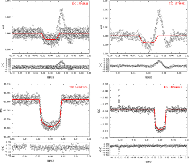
We finally obtained the fitted results and plotted several examples as shown in Figure 11. We reobtained physical parameters of exoplanets, which are listed in Table 7. To compare some of our results with previous results in the literature (e.g., Bakos et al. 2007; Kossakowski et al. 2019; Nielsen et al. 2020; Szabó et al. 2020), we plotted our results and the parameters given in the catalog in Figure 12. For the orbital period, these are the most precise parameters to determine from the tradition light curve. Therefore, their dispersion is very low. The errors of our results are relatively large because TESS has a small aperture of only 9.5 cm. The left panel of the figure shows the relationship between the sum of the orbit radii and the ratio of the semimajor axis of the orbit. The middle panel shows the relationship between the periods of the planets. The right panel shows the ratio of the radius of a planet to the radius of a star, which reflects the reliability of our fitted results, while the accuracy of the calculated data depends on the quality of the light curve. We have listed the other detailed parameters of the fitting in Table 7. In a word, we reproduced and validated the orbital parameters, which confirmed the previous results.
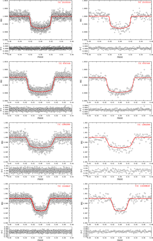
Figure 11. The observational and theoretical light curves, where the circles represent the observation data, and the red line is the fitted result. Left panels are the fitting of the whole light curve. Right panels are one eclipse fitting.
Download figure:
Standard image High-resolution image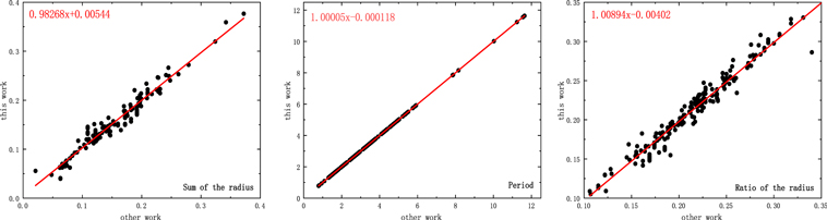
Figure 12. Relationship between our obtained orbital parameters and published data, where the left panel is the sum of the radius, the middle panel is the period, and the right panel is the ratio of the radius of exoplanet and host stars. The red lines represent the linear fit.
Download figure:
Standard image High-resolution imageTable 7. The Revised Parameters for Exoplanet Systems
| TESS ID | Planet Name | R* + Rp | Rp /R* | Inclination | Period | Rp (Earth Radius) | t0 |
|---|---|---|---|---|---|---|---|
| (1) | (2) | (3) | (4) | (5) | (6) | (7) | (8) |
| 14661418 | HATS-22 b | 0.07659 ± 0.00385 | 0.14758 ± 0.00222 | 87.5 ± 0.3 | 3.47447 ± 0.00027 | 10.155 ± 0.039 | 1546.68154 ± 0.00546 |
| 15445551 | WASP-87 b | 0.27229 ± 0.02065 | 0.08937 ± 0.00134 | 81.7 ± 2.0 | 3.75209 ± 0.00047 | 16.297 ± 0.337 | 1843.21862 ± 0.00073 |
| 16740101 | KELT-9 b | 0.35921 ± 0.02825 | 0.08260 ± 0.00109 | 82.4 ± 4.1 | 4.08759 ± 0.00137 | 20.640 ± 0.583 | 1509.89530 ± 0.00046 |
| 17746821 | HAT-P-50 b | 0.22051 ± 0.01889 | 0.08311 ± 0.00168 | 80.7 ± 1.3 | 2.84949 ± 0.00028 | 15.463 ± 0.292 | 1984.68995 ± 0.00032 |
| 86396382 | WASP-12 b | 0.37671 ± 0.01249 | 0.11936 ± 0.00090 | 81.7 ± 1.7 | 4.37781 ± 0.00093 | 22.901 ± 0.286 | 2041.94037 ± 0.00123 |
| 97409519 | WASP-124 b | 0.12768 ± 0.00578 | 0.12922 ± 0.00143 | 85.6 ± 0.4 | 3.53256 ± 0.00025 | 14.361 ± 0.083 | 1578.58488 ± 0.00092 |
| 99834717 | KPS-1 b | 0.17396 ± 0.00943 | 0.11213 ± 0.00172 | 83.1 ± 0.6 | 3.28881 ± 0.00036 | 10.866 ± 0.102 | 1402.78012 ± 0.00054 |
| 100100827 | WASP-18 b | 0.29683 ± 0.01505 | 0.09757 ± 0.00100 | 87.2 ± 4.7 | 2.07280 ± 0.00010 | 12.996 ± 0.196 | 1440.61888 ± 0.00224 |
| 190998418 | Qatar-5 b | 0.14368 ± 0.01402 | 0.10517 ± 0.00224 | 86.1 ± 1.4 | 4.12680 ± 0.00046 | 12.200 ± 0.171 | 1397.40381 ± 0.00040 |
| 191284318 | HAT-P-16 b | 0.15034 ± 0.01304 | 0.10735 ± 0.00187 | 87.2 ± 1.9 | 5.36654 ± 0.00141 | 14.510 ± 0.189 | 1481.06086 ± 0.00075 |
| 198108326 | HAT-P-12 b | 0.1024 ± 0.00602 | 0.14124 ± 0.00227 | 87.9 ± 0.8 | 3.30914 ± 0.00093 | 10.607 ± 0.064 | 1666.01007 ± 0.00144 |
| 198588220 | HAT-P-67 b | 0.21009 ± 0.02187 | 0.08309 ± 0.00160 | 84.9 ± 2.6 | 4.12449 ± 0.00053 | 24.052 ± 0.526 | 2107.34817 ± 0.00066 |
Note. Column (1): TESS ID. Column (2): exoplanet name. Column (3): the ratio of the sum of the radius of the planet and the star to the semimajor axis of the orbit. Column (4): radius ratio of the exoplanet and the host star. Column (5): orbital inclination. Column (6): orbital period. Column (7): exoplanet radius. Column (8): minima time.
Only a portion of this table is shown here to demonstrate its form and content. A machine-readable version of the full table is available.
Download table as: DataTypeset image
6. Livability Judgment
The flares of stars will destroy the atmosphere of planets and affect their habitability. We have made a preliminary judgment on the habitability of the planet through the flare data that we have found. We have made a preliminary judgment on planet habitability of the flare stars found by TESS, Kepler, and K2.
We use the formula given by Lingam & Loeb (2017) to calculate the energy deposited on the exoplanet:

where E is the energy flux from the flare to the exoplanet, Eflare is the energy of the flare, a is the semimajor axis of the orbit, and Rp is the radius of the exoplanet. If we use this formula, it means that we assume that the energy radiated by the flare activity into space is isotropic. However, another point of view is that the flare energy can radiate in a nonisotropic way at an angle of 24° (Melott & Thomas 2012; Neuhäuser & Hambaryan 2014). The energy flux in this case is about 100 times higher than before. Our calculation result uses the second method, so that the energy is E ' ∼ 100E. When the solar flare energy reaches 1035−1036 erg, the ozone layer is predicted to be completely destroyed (Lingam & Loeb 2017). According to this prediction, the surface flux of Earth affected by the flare is determined to be 3.54 × 10⁹ erg cm−2 to 3.54 × 10¹⁰ erg cm−2, and the ozone layer will be completely destroyed. These data help us to determine the threshold of the impact of flare energy on the habitability of exoplanets. At the same time, the planetary atmosphere has a certain recovery ability. For example, after the Carrington flare (5 × 1032 erg; Cliver & Dietrich 2013) in 1859, the global ozone layer fell by an average of 5%. And Earth's atmosphere returned to the state before the event after 48 months (Thomas et al. 2007). When we judge the habitability of exoplanets on the flare scale, we use the maximum flare energy that Earth can bear and its self-recovery rate. For stars with only one flare, we judge by the lowest energy value of the complete destruction of Earth's atmosphere. We have made a preliminary judgment on the habitability of the planets around the flare stars with 3.54 ×10⁹ erg cm−2 as the threshold condition. The actual situation should be lower than this value, mainly for the following two reasons: (1) After the high-energy flare, even if the planetary atmosphere is not completely destroyed, the poor atmospheric environment is not suitable for survival. (2) Due to the limited observed data, some stars have only been observed for a short time, so that only one flare can be found. We are not sure whether their flares are frequent. For stars with multiple flares, we calculate their flare frequency, calculate their average flare energy, and determine whether they are habitable in combination with the recovery level of the planetary atmosphere. If its damage rate is lower than its atmospheric repair rate, it is considered livable. We chose the research of Thomas et al. (2007) on the Carrington event as the standard of planetary recovery atmospheric ability:

where Searth is the repair capacity of Earth's atmosphere, and its units are erg cm−2 s−1. EC is the energy flux of the Carrington event, and t is the atmospheric recovery time of Earth after the Carrington event.

where Sexoplanet is the energy flux density received by exoplanets, tob is the observation duration of observing the star, and Esum is the total energy flux of each flare of each star. When Searth > Sexoplanet, we consider that this exoplanet is livable. Due to the limitations of existing data and observations, the standard for judging habitability that we have developed is relatively low. However, it also has certain advantages, and the real livable star will not be missed. This method can be used to make a preliminary judgment on the habitable star on the scale of flaring. Because it usually requires a longer observation time to predict the flare of a star, especially for some stars with infrequent flares, long-term observations of host stars are needed in order to further determine the habitability of their exoplanets on the scale of a flare.
7. Summary
In this work, we have provided the parameters of host stars and exoplanets and integrated the observational data of different telescopes. We have established some statistical data on the magnetic and chromospheric activity of the host stars through spectra and light curves.
After using the standard line to judge the habitability of exoplanet host stars, we found that 76.70% of them are active stars in low-resolution observations and 67.77% are in medium-resolution observations. However, after detecting a large number of low- and medium-astigmatism spectra, it is found that for random spectra the activity ratio of stars is about 60%. This seems to indicate that the host stars of exoplanets have higher activity, but we still cannot completely rule out the contingency of our samples, which needs to be judged with the help of more data of exoplanet host stars in the future. We also compared the EW of Hα distribution of flare stars and nonflare stars, as shown in Figure 13. For the LAMOST low-resolution data, we calculated the average and median  and Hα EW values of flare and nonflare stars. The average and median values of the Hα EW with flare stars are −1.228 and −1.311, respectively. The corresponding average and median values of EW Hα with nonflare stars are −1.181 and −1.293, respectively. The average value of
  is 7.78 × 10⁻⁵, and the median is 6.60 × 10⁻⁵. The average value of
  is 8.45 × 10⁻⁵, and the median is 7.10 × 10⁻⁵. There are no obvious differences of the
  and Hα EWs for the flare and nonflare stars. Hilton et al. (2010) obtained that the stellar activity of flare stars is higher than that of nonflare stars. They detected the flare events of M stars using the time-resolved spectroscopic observations from SDSS DR6. We detected the flare events using the TESS light curve. This might be caused by the different times of the LAMOST spectrum and the TESS light curve or the limited samples with different stellar parameters. We hope to perform simultaneous observations of photometric and spectroscopic data. We will discuss the relationship between the Hα and flares in the future.

Figure 13. These two pictures show the distribution of the EW of Hα of flare and nonflare stars for low-resolution (left panel) and medium-resolution spectra (right panel). Red circles represent flare stars, and black circles represent nonflare stars.
Download figure:
Standard image High-resolution imageWe found 481, 1886, and 467 flares in the data from TESS, Kepler, and K2, respectively. In these flare events, most of the low-energy flares we found come from TESS data and 1-minute exposure data of Kepler and K2. The light curve of a 30-minute exposure time cannot reflect many changes of a short-term scale. A comparison of the results of the two telescopes shows that the flare energy will increase with the increase of the flare time, which is consistent with the results of Wu et al. (2015). It is generally believed that a flare with energy above 1033 erg is a superflare. Rubenstein & Schaefer (2000) proposed that planet−star interactions will cause superflares of stars. In fact, we found that there are many single-star systems with superflares, and there are no hot Jupiters. This result is consistent with Tu et al. (2020), which indicates that stellar magnetic activity may also cause superflares.
The Hα and flare intensities are almost constant for the Rossby number Ro ≤ 0.12 in the saturated regime and decrease with increasing Ro in the unsaturated regime. These results are consistent with the previous results (Douglas et al. 2014; Fang et al. 2018). We also plotted the relationship between the ratio of flare energy to luminosity and Rossby number in Figure 6. The flare intensity is almost constant for the Rossby number Ro ≤ 0.12 in the saturated regime and decreases with increasing Ro in the unsaturated regime. Our results are consistent with the previous results (Yang & Liu 2019). These also indicate that the trend of the Hα emission versus Ro is consistent with the trend of the flare. The Hα EW parameters can be used as the proxy of the flare events (Chang et al. 2018). In addition, we plotted two different relationships shown in Figure 6. The lower-left panel shows the relationship between the flare amplitude and EW of Hα, while the lower-right panel shows the ratio of flare energy to luminosity and EW of Hα. It can be seen that the Hα emission is positively correlated with the flare activity. These results are consistent with the previous results (Chang et al. 2017; Zhang et al. 2020).
For the part relating to fitting the light curve, we used the JKTEBOP program and TESS data to calculate specific exoplanet parameters and obtained new results. We found some examples of occultation and flare at the same time, as shown in Figure 14. Lanza (2012) explored the interaction between the stellar magnetic field and the planetary magnetic field. Green et al. (2021) also explored the mutual magnetic activities between stars and exoplanets and simulated the influence of the magnetic activity on the atmosphere of exoplanets, which is helpful to the discussion of planet habitability. By calculating the period, magnetic field intensity, and frequency of the flare, Chen et al. (2021) found that the repeated flare activity will affect the atmospheric state of the nearby planets and then stimulate the planetary atmosphere. By carefully screening the data from our work, we assessed the habitability of exoplanets with host stars with flares. According to our criteria, we found 21 habitable planets for 562 stars with flares. These results are shown in Table 8.
Figure 14. Examples of transit light curves with flares, where the left panel is the fitting of the whole light curve and the right panel is one eclipse fitting.
Download figure:
Standard image High-resolution image
Table 8. Habitable Exoplanet Parameters
| OBJECT | Planet Name | tstart | tend | tob | tsum | Rp | Number | Esum | S | Eflux | Livability |
|---|---|---|---|---|---|---|---|---|---|---|---|
| (1) | (2) | (3) | (4) | (5) | (6) | (7) | (8) | (9) | (10) | (11) | (12) |
| EPIC 203570729 | USco1556 b | 2060.273507 | 2139.058393 | 78.784886 | 78.784886 | 3500 | 7 | 3.82E+37 | 1.62E-04 | 1.10E+03 | Y |
| EPIC 203626828 | USco1621 b | 2060.273935 | 2139.058850 | 78.784915 | 78.784915 | 2880 | 2 | 2.93E+37 | 1.83E-04 | 1.25E+03 | Y |
| EPIC 203640875 | ROXs 12 b | 2060.274018 | 2139.058947 | 78.784929 | 78.784929 | 210 | 1 | 1.40E+39 | 1.65E+00 | 1.12E+07 | Y |
| EPIC 203776696 | K2-52 b | 2060.274014 | 2139.058938 | 78.784924 | 78.784924 | 0.0485 | 1 | 3.99E+37 | 8.81E+05 | 6.00E+12 | N |
| KIC 10027247 | Kepler-1229 b | 1337.168012 | 1371.332724 | 34.164712 | 124.504817 | 0.2899 | 3 | 1.08E+34 | 4.25E+00 | 4.57E+07 | N |
| KIC 10000941 | Kepler-1558 b | 1373.477593 | 1471.146990 | 97.669398 | 1166.166135 | 0.0419 | 29 | 3.31E+35 | 6.62E+02 | 6.67E+10 | N |
| KIC 10264660 | Kepler-14 b | 599.187812 | 629.306390 | 30.118578 | 86.145588 | 0.0769 | 4 | 5.80E+34 | 4.66E+02 | 3.47E+09 | N |
| KIC 10272442 | Kepler-657 b | 1182.726729 | 1273.066703 | 90.339974 | 90.339974 | 0.1654 | 1 | 5.44E+34 | 9.01E+01 | 7.03E+08 | N |
| KIC 10878263 | Kepler-414 b | 970.078328 | 1000.278941 | 30.200614 | 64.365382 | 0.0527 | 4 | 3.95E+34 | 9.03E+02 | 5.02E+09 | N |
| KIC 10904857 | Kepler-488 b | 1337.167489 | 1371.331841 | 34.164352 | 34.164352 | 0.0428 | 2 | 1.17E+35 | 7.64E+03 | 2.25E+10 | N |
| KIC 10905746 | Kepler-1651 b | 1274.129434 | 1305.005059 | 30.875625 | 678.615679 | 0.054 | 85 | 4.20E+34 | 8.68E+01 | 5.09E+09 | N |
| KIC 10978763 | Kepler-339 b | 1337.167780 | 1371.332418 | 34.164638 | 63.406156 | 0.0545 | 3 | 4.98E+34 | 1.08E+03 | 5.94E+09 | N |
Note. Column (1): object name. Column (2): exoplanet name. Column (3): observation start time. Column (4): observation end time. Column (5): observation time of one light curve. Column (6): total observation time. Column (7): semimajor axis of planetary orbit. Column (8): number of flares observed. Column (9): total flare energy. Column (10): the flare energy flux density received by the planet of stars with multiple flares, in erg cm−2 s−1. Column (11): the flare energy flux received by the planet of stars with a single flare, in erg cm−2. Column (12): livability judgment.
Only a portion of this table is shown here to demonstrate its form and content. A machine-readable version of the full table is available.
Download table as: DataTypeset image
This research was supported by the China Scholarship Fund, the Joint Fund of Astronomy of the NSFC, and CAS grant Nos. 11963002, U1631236, and U1431114. We would like to thank John Southworth, the author of JKTEBOP, for sharing the program. This paper is based on the data of LAMOST, a National Major Scientific Project built by the Chinese Academy of Sciences. It also includes data collected by TESS mission, Kepler mission, K2 mission, the NASA Astrophysics Data System, and the MAST data archive of the Space Telescope Science Institute. We also acknowledge the fostering project of GuiZhou University with No. 201911. We also acknowledge the support by the science research grants from the China Manned Space Project with No. CMS-CSST-2021-B07 and Cultivation Project for FAST Scientific Payoff and Research Achievement of CAMS-CAS.
Footnotes
- 7
- 8
- 9