Methods for comparing scanpaths and saliency maps: strengths and weaknesses

Abstract

In this article, we are interested in the computational modeling of visual attention. We report methods commonly used to assess the performance of these kinds of models. We survey the strengths and weaknesses of common assessment methods based on diachronic eye-tracking data. We then illustrate the use of some methods to benchmark computational models of visual attention.

Introduction

Eye tracking is a well-known technique for analyzing visual perception and attention shift and assessing user interfaces. However, until now, data analysis from eye-tracking studies has focused on synchronic indicators such as fixation (duration, number, etc.) or saccade (amplitude, velocity, etc.), rather than diachronic indicators (scanpaths or saliency maps). Synchronic means that an event occurs at a specific point in time, while diachronic means that this event is taken into account over time. We focus in this article on diachronic measures and review different ways of analyzing sequences of fixations represented as scanpaths or saliency maps.

Visual scanpaths depend on bottom-up and top-down factors such as the task users are asked to perform (Simola, Salojärvi, & Kojo, 2008), the nature of the stimuli (Yarbus, 1967), and the intrinsic variability of subjects (Viviani, 1990). Being able to measure the difference (or similarity) between two visual behaviors is fundamental both for differentiating the impact of different factors and for understanding what governs our cognitive processes. It also plays a key role in assessing the performance of computational models on overt visual attention, by, for example, evaluating how well saliency-based models predict where observers look.

In this study, we survey common methods for evaluating the difference/similarity between scanpaths and between saliency maps. In the first section, we describe state-of-the-art methods commonly used to compare visual scanpaths. We then consider the comparison methods that involve either two saliency maps or one saliency map plus a set of visual fixations. We first define how human saliency maps are computed and list some of their most important properties. The strengths and weaknesses of each method are emphasized. In the fourth section, we address inter observer variability, which reflects the natural dispersion of fixations existing between observers watching the same stimuli. It is important to understand the mechanisms underlying this phenomenon, since this dispersion can be used as an upper bound for a prediction. To illustrate the latter point and the use of common similarity metrics, we compare ground truth and model-predicted saliency maps. Finally, we broaden the scope of this article by raising a fundamental question: Do all visual fixations have the same meaning and role, and is it possible to classify fixations as being bottom-up, cognitive, top-down, or semantic?

Methods for comparing scanpaths

Different metrics are available for comparing two scanpaths, using either distance-based methods (string edit technique or Mannan distance) or vector-based methods. Distance-based methods compare scanpaths only from their spatial characteristics, while vector-based approaches perform the comparison across different dimensions (frequency, time, etc.). These metrics are more or less complex and relevant depending on the situation to be analyzed. However, there is no consensus in the community on the use of a given metric. In this section, we present three metrics: the string edit metric, Mannan’s metric, and a vector-based metric.

String edit metric

The idea of the string edit metric is that a sequence of fixations on different areas of interest (AOIs) can be translated into a sequence of symbols (numbers or letters) forming strings that are compared. This comparison is carried out by calculating a string edit distance (often called the Levenshtein distance) that gives a measure of the similarity of the strings (Levenshtein, 1966). This technique was originally developed to account for the edit distance between two words, and the measured distance is the number of deletions, insertions, or substitutions that are necessary for the two words to be identical (which is also called the alignment procedure). This metric takes as input two strings (coding AOIs) and computes the minimum number of edits needed to transform one string into the other. A cost is associated with each transformation and each character. The goal is to find a series of transformations that minimizes the cost of aligning one sequence with the other. The total cost is the edit distance between the two strings. When the cost is minimal, the similarity between the two strings is maximal (i.e., when the two strings are identical, the distance is equal to 0). Conversely, the distance increases with the cost and, therefore, with the dissimilarity between the two strings. Figure 1 illustrates the method. The Levenshtein distance is the most common way to compare scanpaths (Josephson & Holmes, 2002; Privitera & Stark, 2000) and has been widely used for assessing the usability of Web pages (Baccino, 2004).

Fig. 1

Computation of a string edit distance to align the sequences ABCDE and ABAA recorded on a Web page. First, areas of interest are segmented and coded by letters (A, B, C . . .). Second, the substitution operations are carried out. The total cost is equal to 3 (the minimum number of substitutions) and normalized to the length of the longer string—here, 5—yielding an edit distance between the two strings of d = (1 − 3/5) = 0.4

The string edit distance can be computed using a dynamic programming technique (the WagFish algorithm (Wagner & Fischer, 1974)) that incrementally computes optimal alignments (minimizing the cost). The Levenshtein distance is not the only string edit distance that can be used for scanpaths. Others are described below:

• LCS is the length of the longest common subsequence, which represents the score obtained by allowing only addition and deletion, not substitution;

• Damerau-Levenshtein distance allows addition, deletion, substitution, and the transposition of two adjacent characters; and

• Hamming distance allows only substitution (and hence, applies only to strings of the same length).

The advantage of the string edit technique is that it is easily computed and keeps the order of fixations. It is also possible to compare observed scanpaths with predicted scanpaths when certain visual profiles are expected from the cognitive model used by the researcher (Chanceaux, Guérin-Dugué, Lemaire, & Baccino, 2009). However, several drawbacks have to be underlined:

• Since the string edit is based on a comparison of the sequence of fixations occurring in predefined AOIs, the question is how to define these AOIs. There are two ways: automatically gridded AOIs or content-based AOIs. The former is built by putting a grid of equally sized areas across the visual material, but for the latter, the meaningful regions of the stimulus need to be subjectively chosen. Whatever AOIs are constructed, the string edit method means that only the quantized spatial position of the visual fixations are taken into account. Hence, some small differences in scanpaths may change the string, while others produce the same string.

• The string edit method is limited when certain AOIs have not been fixated, so there is a good deal of missing data.

Mannan’s metric

The Mannan distance (Mannan, Ruddock, & Wooding, 1995, 1996, 1997) is another metric comparing scanpaths, but on the basis of their spatial properties rather than their temporal dimensions, in the sense that the order of fixations is completely ignored. The Mannan distance compares the similarity between scanpaths by calculating the distance between each fixation in one scanpath and its nearest neighbor in the other scanpath. A similarity index (Is) represents the average linear distance between two scanpaths (D), with randomized scanpaths having the same size (Dr). These randomly generated scanpaths are used for weighting the sequence of real fixations, taking into account the fact that real scanpaths may convey a randomized component. The similarity index (Is) is given by

$$ Is = \left[ {1 - \frac{D}{{Dr}}} \right] \times 100 $$

D is a measure of distance given by

${D^2} = \frac{{{n_1}\sum\nolimits_{j = 1}^{{n_2}} {d_{2j}^2} }}{{2{n_1}{n_2}\left( {{a^2} + {b^2}} \right)}} + \frac{{{n_2}\sum\nolimits_{i = 1}^{{n_1}} {d_{1i}^2} }}{{2{n_1}{n_2}\left( {{a^2} + {b^2}} \right)}}$

where,

• n ₁ and n ₂ are the number of fixations in the two traces;

• d _1i is the distance between the ith fixation in the first trace and its nearest neighbor in the second trace;

• d _2j is the distance between the jth fixation in the second trace and that of its nearest neighbor in the second one;

• a and b are the side lengths of the image; and

• Dr is the distance between two sets of random locations.

The values returned by the algorithm (Is) range from 0 (random scanpath) to 100 (identity). The main drawbacks of this technique are the following:

• The Mannan distance does not take into account the temporal order of fixation sequence. This means that two sequences of fixations having a reversed order but with an identical spatial configuration give the same Mannan distance.

• A difficult problem occurs when the two scanpaths have very different size (the number of fixations between them is very different). The Mannan distance may show a great similarity while the shapes of the scanpaths are definitely different. The Mannan distance is not tolerant to high variability between scanpaths.

Vector-based metric

An interesting method was recently proposed by Jarodzka, Holmqvist, and Nystr (2010). Each scanpath is viewed as a sequence of geometric vectors that correspond to subsequent saccades of the scanpath. The vector representation shows the length and the direction of each saccade. A saccade is defined by a starting position (fixation n) and ending position (fixation n + 1). Then a scanpath with n fixations is represented by a set of n − 1 vectors, and several properties can therefore be preserved, such as the shape of the scanpath, the scanpath length, and the position and duration of fixations. The sequences that have to be compared are aligned according to their shapes (although this alignment can be performed on other dimensions: length, durations, angle, etc.).

Each vector of one scanpath corresponds to one or more vectors of another scanpath, such that the path in the matrix of similarity between the vectors going from (1, 1) (similarity between the first vectors) to (n, m) (similarity between the last vectors) is the shortest one. Once the scanpaths are aligned, various measures of similarity between vectors (or sequences of vectors) can be used, such as average difference in amplitude, average distance between fixations, and average difference in duration.

For example, Fig. 2 shows two scanpaths A and B (the first saccade is going upward). The alignment procedure attempts to match the five vectors (for the five consecutive saccades) of the subject scanpath with the four vectors of the model scanpath. Saccades 1 and 2 of scanpath A are aligned with saccade 1 of scanpath B, saccade 3A is aligned with saccade 2B, etc. Once the scanpaths are aligned, similarity measures are computed for each alignment. Jarodzka et al.’s (2010) procedure ends up with five measures of similarity (difference in shape, amplitude, and direction between saccade vectors, distance between fixations, and fixation durations).

Fig. 2

Alignment using saccadic vectors. The alignment procedure attempts to match the five vectors of the two scanpaths. The best match is the following: 1 – 2/1; 3/2; 4/3; 5/4 – 5

This vector-based alignment procedure has a number of advantages over the string edit method. The first is that it does not need to determine predefined AOIs (and is, therefore, not dependent on a quantization of space). The second one is that it can align scanpaths not only on the spatial dimension, but also on any dimension available in saccade vectors (angle, duration, length, etc.). For example, Lemaire, Guérin-Dugué, Baccino, Chanceaux, and Pasqualotti (2011) used the spatial distance between saccades, the angle between saccades, and the difference of amplitude to realize the alignment. Third, this alignment technique provides more detailed information on the type of (dis)similarity of two scanpaths according to the dimensions chosen. Lastly, the new measure deals with temporal issues, not only fixation durations, but it also successfully deals with shifts in time and variable scanpath lengths. The major drawbacks are the following:

• This measure compares only two scanpaths. Sometimes, the overall aim is to compare whole groups of subjects with each other.

• It is presumed that fixations and saccades must occur. Other eye movements such as smooth pursuit are not handled. Smooth pursuit movements are important when a video is watched. However, the problem may be solved if it is possible to represent smooth pursuit as a series of short vectors that are not clustered into one long vector.

• This alignment procedure is independent of the stimulus content. However, the chosen dimensions may be weighted by some semantic values carefully selected by the researcher.

Methods for comparing saliency maps

Comparing two scanpaths requires taking a number of factors, such as the temporal dimension or the alignment procedure, into account. To overcome these problems, another kind of method can be used. In this section, we focus on approaches involving two bidimensional maps. We first briefly describe how the visual fixations are used to compute a continuous saliency map. Second, we describe three common methods used to evaluate the degree of similarity between two saliency maps: a correlation-based measure, the Kullback–Leibler divergence, and receiver operating characteristic (ROC) analysis.

From a discrete fixation map to a continuous saliency map

A discrete fixation map f ⁱ for the ith observer is classically defined as

$$ {f^i}(x) = \sum\limits_{k \,= \,1}^M {\delta \left( {x - {x_f}(k)} \right)} $$

where x is a vector representing the spatial coordinates and x _f (k) is the spatial coordinates of the kth visual fixation. The value M is the number of visual fixations for the ith observer. $\delta \left( \cdot \right)$ is the Kronecker symbol (δ(t) = 1 if t = 1; otherwise, δ(t) = 0).

For N observers, the final fixation map f is given by

$$ f(x) = \frac{1}{N}\sum\limits_{i = 1}^N {{f^i}(x).} $$

A saliency map S is then deduced by convolving the fixation map f by an isotropic bidimensional Gaussian function

$$ S(x) = f(x) * {G_\sigma }(x) $$

where σ is the standard deviation of the Gaussian function. It is commonly accepted that σ should be set to 1° of visual angle. One degree of visual angle represents an estimate of the size of the fovea. The standard deviation depends on the experimental setup (size of the screen and viewing distance). It is also implicitly assumed that a fixation can be approximated by a Gaussian distribution (Bruce & Tsotsos, 2006; Velichkovsky, Pomplum, Rieser, & Ritter, 1996). An example of fixation and saliency maps is given by Fig. 3. A heat map, which is a simple colored representation of the continuous saliency map, is also shown. Red areas pertain to salient areas, whereas blue areas are for nonsalient areas. Note that the fixation map illustrated by Fig. 3 is not exactly the one defined by the previous formula.

Fig. 3

From left to right: a original, b fixation map with red fixation points, c heat map (red spots represent the most visually salient areas of the picture), and d saliency map

Throughout this section, we use the two continuous saliency maps shown in Fig. 4 to illustrate the comparison methods. Both maps are obtained from visual fixations of 3 observers.

Fig. 4

Heat maps and continuous saliency maps obtained from fixations of two groups of 3 observers

Fixation duration is not taken into account in the computation of the continuous saliency map. Itti (2005) showed that there was no significant correlation between model-predicted saliency and duration of fixation. Fixation duration is often considered to reflect the depth and the speed of visual processing in the brain. The longer the fixation duration, the deeper the visual processing (Henderson, 2007; Just & Carpenter, 1976). Total fixation time (the cumulative duration of fixations within a region) can be used to gauge the amount of total cognitive processing engaged with the fixated information (Rayner, 1998). There are a number of factors that influence the duration of fixations. Among these factors, the visual quality of the displayed stimuli plays an important role, as suggested by Mannan et al.’s (1995) experiment. They presented filtered and unfiltered photos to observers and reported a significant increase in the fixation duration for the filtered photos. Another factor is related to the number of objects present in the scene. Irwin and Zelinsky (2002) observed that the duration of fixations increases with the number of objects in the scene.

Correlation-based measures

The Pearson correlation coefficient r between two maps H and P is defined as

$$ {r_{H,P}} = \frac{{cov\left( {H,P} \right)}}{{{\sigma_H}{\sigma_P}}} $$

where cov (H, P) is the covariance between H and P and σ _H and σ _P represent the standard deviation of maps H and P, respectively.

The linear correlation coefficient has a value between −1 and 1. A value of 0 indicates that there is no linear correlation between the two maps. Values close to 0 indicate a poor correlation between the two sets. A value of 1 indicates a perfect correlation. The sign of r is helpful in determining whether data share the same structure. A value of −1 also indicates a perfect correlation, but the data vary together in opposite directions.

This indicator is very simple to compute and is invariant to linear transformation. Several studies have used this metric to assess the performance of computational models of visual attention (Jost, Ouerhani, von Wartburg, Mauri, & Haugli, 2005; Le Meur, Le Callet, Barba, & Thoreau, 2006; Rajashekar, van der Linde, Bovik, & Cormack, 2008). Correlations are usually reported with degrees of freedom (the total population minus 2) in parentheses and the significance level. For instance, the two continuous saliency maps illustrated by Fig. 4 are strongly correlated, r ( 393214 ) = .826, p < .001.

Note that the Spearman's rank correlation can also be used to measure the similarity between two sets of data (Toet, 2011).

The Kullback–Leibler divergence

The Kullback–Leibler (KL) divergence is used to estimate the overall dissimilarity between two probability density functions. Let us define two discrete distributions R and P with probability density functions r _k and p _k . The KL-divergence between R and P is given by the relative entropy of P with respect to R:

$$ KL\left( {R,P} \right) = \sum\nolimits_k {{p_k}log} \frac{{{r_k}}}{{{p_k}}}. $$

The KL-divergence is defined only if r _k and p _k both sum to 1 and if r _k > 0 for any k such that p _k > 0.

The KL-divergence is not a distance, since it is not symmetric and does not satisfy the triangle inequality. The KL-divergence is nonlinear. It varies in the range of zero to infinity. A zero value indicates that the two probability density functions are strictly equal. The fact that the KL-divergence does not have a well-defined upper bound is a strong drawback.

In our context, we have to compare two bidimensional saliency maps (H and P). We first transform these maps into two bidimensional probability density functions by dividing each location of the map by the sum of all pixel values. The probability that an observer focuses on position x is given by:

$$ \matrix{ {{p_H}(x) = \frac{{H(x) + \in }}{{\sum\nolimits_i {\left( {H(i) + \in } \right)} }}} \\ {{p_P}(x) = \frac{{P(x) + \in }}{{\sum\nolimits_i {\left( {P(i) + \in } \right)} }}} \\ }<!end array> $$

where ϵ is a small constant to avoid division by zero.

If we consider the example of Fig. 4, we compute the KL-divergence by first considering the saliency map (b) as the reference and, second, the saliency map (d) as the reference. We obtain KL = 3.33 and KL = 7.06, respectively. Since the KL-divergence is not a distance, the results are not the same. They indicate that the overall dissimilarity is highest when the continuous saliency map (d) is taken as the reference.

Receiver operating characteristic analysis

The ROC analysis (Green & Swets, 1966) is probably the most popular and most widely used method in the community for assessing the degree of similarity of two saliency maps. ROC analysis classically involves two sets of data: The first is from the ground truth (also called the actual values), and the second is the prediction (also called the outcomes).

Here, we perform ROC analysis between two maps. It is also common to encounter a second method in the literature that involves fixation points and a saliency map. This method is described in the Hybrid Methods section.

Continuous saliency maps are processed as a binary classifier applied on every pixel. It means that the image pixels of the ground truth, as well as those of the prediction, are classified as fixated (or salient) or as not fixated (or not salient). A simple threshold operation is used for this purpose. However, two different processes are used depending on whether the ground truth or the prediction is considered:

• Thresholding the ground truth: The continuous saliency map is thresholded with a constant threshold in order to keep a given percentage of image pixels. For instance, we can keep the top 2 %, 5 %, 10 %, or 20 % salient pixels of the map, as illustrated by Fig. 5. This threshold is called $T_G^x$ (G for the ground truth and x indicating the percentage of image considered as being fixated).

  Fig. 5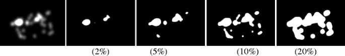

  

  Thresholded saliency maps to keep the top percentage of salient areas. From left to right: 2 %, 5 %, 10 %, and 20 %

• Thresholding the prediction: The threshold is systematically moved between the minimum and the maximum values of the map. A high-threshold value corresponds to an overdetection, whereas a smaller threshold affects the most salient areas of the map. This threshold is called $T_P^x$ (P for the prediction and x indicating the ith threshold).

For each pair of thresholds, four numbers featuring the quality of the classification are computed. They represent the true positives (TPs), the false positives (FPs), the false negatives (FNs), and the true negatives (TNs). The true positive number is the number of fixated pixels in the ground truth that are also labeled as fixated in the prediction.

Figure 5 gives an illustration of the thresholding operation on the parrot picture (Fig. 3). The first continuous saliency map (b) of Fig. 4 is thresholded to keep 20 % of the image ($T_G^{20}$) and is compared with the second continuous saliency map (d) of Fig. 4. The classification result is illustrated by Fig. 6. The red and uncolored areas represent pixels having the same label—that is, a good classification (TP). The green areas represent the pixels that are fixated but are labeled as nonfixated locations (FN). The blue areas represent the pixels that are nonfixated but are labeled as fixated locations (FP). A confusion matrix is often used to visualize the algorithm’s performance (see Fig. 7c).

Fig. 6

Classification result (on the right) when a 20 % thresholded ground truth (left picture) and a prediction (middle picture) are considered. Red areas are true positives, green areas are false negatives, and blue areas are false positives. Other areas are true negatives

Fig. 7

Pseudo-code to perform an ROC analysis between two maps (a), ROC curve (b), and the confusion matrix (c). The AUC is approximated here by a left Riemann sum as illustrated in panel b

An ROC curve that plots the FP rate (FPR) as a function of the TP rate (TPR) is usually used to display the classification result for the set of thresholds used. The TPR, also called sensitivity or recall, is defined as TPR = TP/(TP + FN), whereas the FPR is given by FPR = FP/(TP + FN). The ROC area, or the area under curve (AUC), provides a measure indicating the overall performance of the classification. A value of 1 indicates a perfect classification. The chance level is .5. The ROC curve of Fig. 6 is given in Fig. 7. There are different methods to compute the AUC. The simplest ones are based on the left and right Riemann sums. The left Riemann sum is illustrated by Fig. 7. A more efficient approximation can be obtained by a trapezoid approximation: Rather than computing the area of rectangles, the AUC is given by summing the area of trapezoids. In our example, the AUC value is 0.83.

Hybrid methods

So far, we have focused on similarity metrics involving two scanpaths or two saliency maps. In this section, we describe methods based on a saliency map and a set of fixation points. We call this kind of method hybrid since it mixes two types of information. Four approaches are presented: ROC analysis, normalized scanpath saliency, percentile, and the Kullback–Leibler divergence.

Receiver operating characteristic analysis

The ROC analysis is performed here between a continuous saliency map and a set of fixations. The method tests how the saliency at the points of human fixation compares with the saliency at nonfixated points. As in the previous section, the continuous saliency map is thresholded to keep a given percentage of pixels of the map. Each pixel is then labeled as either fixated or not-fixated. For each threshold, the observer’s fixations are laid down on the thresholded map. The TPs (fixations that fall on fixated areas) and the FNs (fixations that fall on nonfixated areas) are determined (as illustrated by Fig. 8). A curve that shows the TPR (or hit rate) as a function of the threshold can be plotted. Note that the percentage of the image considered to be salient is in the range of 0 %–100 %. If the fixated and nonfixated locations cannot be discriminated, the AUC will be 0.5. This first analysis method is used in studies such as Tatler, Baddeley, and Gilchrist (2005) and Torralba, Oliva, Castelhano, and Henderson (2006). Although interesting, this method is not sensitive to the false alarm rate.

Fig. 8

Example of ROC analysis. Red and green dots are the fixations of 2 observers for the parrots image. These dots are drawn on a thresholded saliency map. On the left-hand side, the hit rate is 100 %, whereas the rate is 50 % for the example on the right-hand side

To deal with the previous limitation, a set of control points, corresponding to nonfixated points, can be generated. Two methods commonly encountered in the literature are discussed. The first method is the simplest one and consists in selecting control points from either a uniform or a random distribution. This solution does not take into account the fact that fixations are distributed neither evenly nor randomly throughout the scene, as illustrated by Fig. 9. The second method, proposed by Einhauser and Konig (2003) and Tatler et al. (2005), defines control points by choosing locations randomly from a distribution of all fixation locations that occurred at the same time, but on other images. This way to define the control point is important for different reasons. First, since the fixations come from the same observer, so the same bias, systematic tendency, or peculiarity of the observer are taken into account. This is illustrated by Fig. 10. These factors then have a limited influence on the classification results. Among them, the most important influence is the central bias illustrated in Fig. 9. A number of factors can explain this central tendency. The center might reflect an advantageous viewing position for extracting visual information (Renninger, Verghese, & Coughlan, 2007; Tatler, 2007). However, Tatler noted that the distribution of low-level visual features over the picture has no significant impact on this bias. In addition, this tendency to look at the center of images is particularly difficult to remove. Different strategies were tried by Bindemann (2010) to reduce this bias, but without success. This author concluded that the screen-based central fixation bias might be an inescapable feature of scene viewing under laboratory conditions. Second, the set of control points has to stem from the same time interval as the set that is analyzed. Indeed, bottom-up and top-down influences are not similar over time. For instance, bottom-up influences are maximal just after the stimulus onset. Top-down influences tend to increase with viewing time, leading to a stronger dispersion between observers (see the Measuring a Realistic Upper Bound section). Although the second method is more robust than the first one, the method has a serious flaw. It underestimates the salience of areas which are more or less centred in the image.

Fig. 9

Distribution of the first five fixations for 5 observers, combined across seven pictures (top of figure)

Fig. 10

The red dots correspond to the visual fixations of 1 observer viewing the parrots image. Other colors correspond to fixations of the same observer, but for three different pictures. Control fixations are chosen from this set of fixations

In a similar fashion to the method in the Receiver Operating Characteristic Analysis section, the control points and the fixation points are then used to plot an ROC curve. For each threshold, the observer’s fixations and the control ones are laid down on the thresholded map. The TPR (fixations that fall on fixated areas) and the FPR are determined. From this ROC curve, the AUC is computed. The confidence interval is computed by using a nonparametric bootstrap technique (Efron & Tibshirani, 1993). Many samples having the same size as the original set of human fixations are generated by sampling with replacement. These samples are called bootstrap samples. In general, 1,000 bootstrap samples are created. Each bootstrap sample is used as a set of control fixations. The ROC area between the continuous saliency map and the points of human fixation plus the control points is computed. The bootstrap distribution of each ROC analysis is computed, and a bootstrap percentile confidence interval is determined by percentiles of the bootstrap distribution, leaving off $\frac{a}{2} \times 100\%$ of each tail of the distribution where α is the confidence level.

Sometimes, the quality of the classification relies on the equal error rate (EER). The EER is the location on an ROC curve where the FPR and the TPR are equal (i.e., the error at which false alarms equal the miss rate FPR = 1 − TPR). As with the AUC, the EER is used to compare the accuracy of the prediction. In general, the system with the lowest EER is the most accurate.

Normalized scanpath saliency

The normalized scanpath saliency (NSS; Peters, Iyer, Itti, & Koch, 2005) is a metric that involves a saliency map and a set of fixations. The idea is to measure the saliency values at fixation locations along a subject’s scanpath.

The first thing to do is to standardize the saliency values in order to have a zero mean and unit standard deviation. It is simply given by

$$ {Z_{SM}}(x) = \frac{{SM(x) - \mu }}{\sigma } $$

where Z _SM is the standardized saliency map and

$$ \matrix{ {\mu = \frac{1}{{\left| I \right|}}\sum\limits_{t \in I} {SM\left( {{x_t}} \right)} } \\ {\sigma = \sqrt {{\frac{1}{{\left| I \right|}}\sum\limits_{t \in I} {{{\left( {SM\left( {{x_t}} \right) - \mu } \right)}^2}} }} } \\ }<!end array> $$

where the operator $\left| \cdot \right|$ indicates the number of pixels of the picture. For a given coordinate, the quantity Z _SM (x _i ) represents the distance between the saliency value at x _i and the average of saliency expressed in units of the standard deviation. This value is negative when the saliency value at the fixation locations is below the mean, positive when above. To take account of the fact that we do not focus accurately on a particular point, the NSS value for a given fixation location is computed on a small neighborhood centered on that location:

$$ NSS\left( {{x_f}(k)} \right) = \sum\limits_{j \in \pi } {{K_h}\left( {{x_f}(k) - {x_j}} \right){Z_{SM}}\left( {{x_j}} \right)} $$

where K is a kernel with a bandwidth h and π is a neighborhood.

The NSS is the average of NSS (x _f (k)) for all fixations M of an observer. It is given by

$$ NSS = \frac{1}{M}\sum\nolimits_{k = 1}^M {NSS\left( {{x_f}(k)} \right)} . $$

Figure 11 illustrates the computation of the NSS value for a scanpath composed of eight visual fixations. In this example, the average NSS value is 0.3, indicating a good correspondence between the model-predicted saliency map and the observer’s scanpath.

Fig. 11

Example of normalized scanpath saliency computation. The heat map is a normalized version of the model-predicted saliency map with a zero mean and unit standard deviation. A scanpath composed of eight fixations (gray circles; the black one is the first fixation) is overlaid upon the standardized map. The normalized salience is extracted for each location. Values are shown in black next to the fixations

Percentile

In 2008, Peters and Itti designed a metric called percentile (Peters & Itti, 2008). A percentile value P(x _f (k)) is computed for each location of fixation points x _f (k). This score is the ratio between the number of locations in the saliency map with values smaller than the saliency value at point x _f (k) and the set of all locations. The percentile value is defined as follows:

$$ P\left( {{x_f}(k)} \right) = 100 \times \frac{{\left| {\left\{ {x \in X:SM(x) < SM\left( {{x_f}(k)} \right)} \right\}} \right|}}{{\left| {SM} \right|}} $$

where X is the set of locations of the saliency map SM and x _f (k) is the location of the kth fixation. $\left| \cdot \right|$ indicates set size.

The final score is the average of P (x _f (k)) for all fixations of an observer. By definition, the percentile metric has a well-defined upper bound (100 %) indicating the highest similarity between fixation points and saliency map. The chance level is 50 %.

The Kullback–Leibler divergence

The KL-divergence, defined in The Kullback–Leibler Divergence section, is used here to compute the dissimilarity between the histogram of saliency sampled at eye fixations and that sampled at random locations. Itti and Baldi (2009) were the first to use this method. The set of control points (or the set of nonfixated points) are drawn from a uniform spatial distribution. However, human fixations are not randomly distributed, since they are governed by various factors such as the central bias explained earlier. To be more agnostic to this kind of mechanism, Zhang, Tong, Marks, Shan, and Cottrell (2008) measured the KL-divergence between the saliency distribution of fixated points of a test image and the saliency distribution at the same pixel locations but of a randomly chosen image from the test set. To evaluate the variability of the score, the evaluation was repeated 100 times with 100 different sets of control points.

Contrary to the previous KL-divergence method in The Kullback–Liebler Divergence section, a good prediction has a high KL-divergence score. Indeed, as the reference distribution represents chance, the saliency computed at human-fixated locations should be higher than that computed at random locations.

Measuring a realistic upper bound

Most of the methods mentioned above have a well-defined theoretical upper bound. When the performance of a computational model is assessed, it is then reasonable to seek to approach this upper bound. For instance, according to the ROC analysis, an AUC equal or close to one would indicate a very good performance. In our context, this goal is almost impossible to reach. Indeed, there is a natural dispersion of fixations among different subjects looking at the same image. This dispersion (also called inter observer congruency [IOC¹]) is contingent upon a number of factors. First, Tatler et al. (2005) showed that the consistency between visual fixations of different subjects is high just after the stimulus onset but progressively decreases over time. Among the reasons that might explain this variability, the most probable one concerns the time course of bottom-up and top-down mechanisms. Just after the stimulus onset, our attention is mostly steered by low-level visual features, whereas top-down mechanisms become more influential after several seconds of viewing. The second factor concerns the visual content itself. In the case where there is nothing that stands out from the background, the IOC would be small. On the contrary, a visual scene composed of salient areas would presumably attract our visual attention, leading to high congruency. The presence of particular features, such as human faces, human beings, or animals, tends to increase the consistency between observers. A number of studies have shown that we are able to identify and recognize human faces and animals very quickly in a natural scene (Delorme, Richard, & Fabre-Thorpe, 2010; Rousselet, Macé, & Fabre-Thorpe, 2003). Whereas human faces and animals have the ability to attract our attention, decreasing the dispersion between observers, this ability is modulated by novelty or even emotion. Althoff and Cohen’s (1999) study is a good example of this point. They investigated the effect of memory or prior experience on eye movements. They found that visual scanpaths made when famous faces were viewed were more variable than those made when nonfamous faces were viewed. A third factor that could account for the variance between people might be related to cultural differences. Nisbett (2003) compared the visual scan pattern of American and Asian populations. He found that Asian people tend to look more at the background and spend less time on focal objects than do American people. However, a recent study casts doubt on the influence of cultural differences on oculomotor behavior (Rayner, Castelhano, & Yang, 2009).

The IOC can be measured by using a one-against-all approach, also called leave one out (Torralba et al., 2006). It consists in computing the degree of similarity between the fixations of one observer and those of the other subjects. The final value is obtained by averaging the degree of similarity over all subjects.

In this article, the ROC metric is used to compute the degree of similarity, as proposed by Torralba et al. (2006). The first step consists of building a saliency map from the visual fixations of all observers except one (the ith observer). This map is thresholded so that the most fixated areas are set to 1 and the other areas are set to 0. To assess the degree of similarity between the ith observer and the other subjects, the hit rate (as described in the Reciever Operating Characteristic Analysis section)—that is, the percentage of fixations that fall into the fixated regions—is computed. Iterating over all subjects and averaging the scores gives the IOC. Figure 12 illustrates this method.

Fig. 12

Inter observer congruency measurement. On the left, spatial coordinates of visual fixations for each observer are given. By considering all fixations except those from the ith observer, a heat map is computed (on the right). After an adaptive binarization, we count the number of fixations of the ith observer that fall into salient regions (white regions on the bottom image)

Figure 13a illustrates the IOC computation as a function of the numbers of fixations for two different pictures. The first picture (parrots) represents two parrots that are visually salient. The second picture (stream) is a mountain landscape where no element strongly attracts our attention. For both pictures, the congruency decreases over time, as expected. The highest congruency, observed at the beginning of the viewing, is likely to be due to the bottom-up influences and the central bias. It is interesting to emphasize that the congruency for the parrots image is significantly higher than that observed for the stream image. This observation is mainly due to the attractiveness of the two contents. When there is nothing in the scene that catches our attention, observers are not “unconsciously-constrained,” and they just do not explore the visual scene in the same way. Figure 13b, extracted from Le Meur, Baccino, and Roumy (2011), shows other examples of IOC values.

Fig. 13

Inter observer congruency (IOC) as a function of the number of fixations for two different pictures. a Error bars represent the standard error of the mean. b Examples of IOC extracted from pictures used by Le Meur, Baccino, and Roumy (2011)

Assessing the IOC is fundamental to evaluating the performance of the saliency algorithm, although this is overlooked most of the time. An absolute score between a set of fixations and a predicted map is interesting but is not sufficient to draw any conclusions. A low score of prediction does not systematically indicate that the saliency model performs poorly. Such a statement would be true if the dispersion between the observers is low, but false otherwise. Therefore, it is much more relevant to compare the performance of computational models to the IOC (Judd, Ehinger, Durand, & Torralba, 2009; Torralba et al., 2006) or to express the performance directly by normalizing the similarity score by the IOC (Zhao & Koch, 2011). The normalized score would be close to 1 for a good prediction.

Example: performance of state-of-the-art computational models

In this section, we examine the performance of the most prominent saliency models that have been proposed in the literature. The quality of the predicted saliency maps is given here by two metrics: the hit rate (see the Receiver Operating Characteristic Analysis section) and the NSS (see the Normalilzed Scanpath Saliency section). These metrics are hybrid metrics, since they involve a set of visual fixations and a map. We believe that these metrics are the best way to assess the relevance of a predicted saliency map. As compared with saliency map-based methods, hybrid methods are nonparametric. Human saliency maps are obtained by convolving a fixation map by a 2-D Gaussian function, which is parameterized by its mean and its standard deviation. Note that instead of using the hit rate, we could have used an ROC analysis.

To perform the analysis, we use two eye-tracking data sets that are available on the Internet. They are described in the Eye-Tracking Data Sets section. We present and comment on each model’s performance in the Benchmark section.

Eye-tracking data sets

Eye tracking is nowadays a common solution for studying visual perception. Since 2000, some eye-tracking data can be freely downloaded from the Internet for scientific purposes. Table 1 gives the main characteristics of the most important data collections on the Web. They are composed of stimuli that represent landscape, outdoor, or indoor scenes. Some of them are composed of high-level information such as people, faces, animals, and text.

Table 1 Eye-tracking data sets freely available on the Web

These data sets can be used to evaluate the performance of computational models. There is only an implicit consensus on how to set up an eye-tracking test. There is no document that accurately describes what must be done and what must be avoided in the experimental setting. For instance, should observers perform a task when viewing stimuli or not? Do the methods used to identify fixations and saccades from the raw eye data give similar results? We have to be aware that these data sets have been collected in different environments and with different apparatus and settings. To evaluate the performance of saliency models, it is highly recommended that more than one data set be used in order to strengthen the findings.

Benchmark

We compare the performance of four state-of-the-art models: Itti’s model (Itti, Koch, & Niebur, 1998), Le Meur’s model (Le Meur et al., 2006), Bruce’s model (Bruce & Tsotsos, 2009), and Judd’s model (Judd et al., 2009). (For a brief review of saliency models, see Le Meur & Le Callet, 2009.)

Two eye-tracking data sets (Le Meur and Bruce; see Table 1) are used. The degree of similarity between ground truth and model-predicted saliency is evaluated by using the ROC analysis (hit rate) and the NSS metric. Figure 14 gives the ROC curve indicating the performance of different saliency models averaged over all testing images. The method used here is the method described at the beginning of the Receiver Operating Characteristic Analysis section. The upper bound—that is, the inter observer variability—was computed by the method proposed by Torralba et al. (2006) and described in the Measuring a Realistic Upper Bound section. Table 2 gives the average NSS value over the two tested data sets.

Fig. 14

Models performance tested on a the Le Meur data set (top) and b the Bruce data set (bottom). All models perform better than chance and worse than humans. Judd’s model gives the best performance, on average

Table 2 NSS scores for four state-of-the-art saliency models on the Le Meur and Bruce data sets

Under the ROC metric, Judd’s model has the highest performance, as is illustrated by Fig. 14. This result was expected, since this model uses specific detectors (face detection, for instance) that improve the ability to detect salient areas. In addition, this model uses a function to favor the center of the picture in order to take the central bias into account. However, the results are more contrasted under the NSS metric shown in Table 2. On average, across both databases, Judd’s model is still the highest performing. On Bruce’s data set, Itti’s model performs the best, with a value of 0.99, whereas Judd’s model performs at 0.87. The model ranking is therefore dependent on the metric used. It is therefore fundamental to use more than one metric when assessing the performance of computational models of visual attention.

Limitation: Do visual fixations have the same meaning?

Current computational models of visual attention focus on identifying fixated locations of salient areas. From an input picture, a model computes a topographic map indicating the most visually interesting parts. This prediction is then compared with ground truth fixations. The evaluation methodology seems to be appropriate. Unfortunately, an important point is overlooked. By doing this kind of comparison, most researchers have implicitly assumed that fixations, whatever their durations, saccade amplitudes, and start-times, are all similar. In this section, we emphasize the fact that different populations of fixations may exist.

Fixations differ in both their durations and their saccade amplitudes during real-world scene viewing. Antes (1974) was among the first researchers to report these variations. He observed that fixation duration increases while saccade size decreases over the course of scene inspection. This early observation was confirmed by a number of studies (Over, Hooge, Vlaskamp, & Erkelens, 2007; Tatler & Vincent, 2008). The variation in the duration of visual fixations is contingent upon factors such as the quality of the stimulus and the number of objects in the scene (as explained in the From a Discrete Fixation Map to a Continuous Saliency Map section). However, this variance might be explained by functional differences in the fixations. To investigate this point, Velichkovsky and colleagues (Unema, Pannasch, Joos, & Velichkovsky, 2005; Velichkovsky, 2002) conjointly analyzed the fixation duration and the subsequent saccade amplitude. They found a nonlinear distribution indicating that (1) short fixations are associated with long saccades and, conversely, (2) longer fixations are associated with shorter saccades (Fig. 6 in Unema et al., 2005). This dichotomy permits us to disentangle focal-ambient fixations, using the terminology introduced by Trevarthen in 1968. Ambient processing is characterized by short fixations associated with long saccades. This mode might be used to extract contextual information in order to identify the whole scene. Focal processing is characterized by long fixations with short saccades. This mode may be related to recognition and conscious understanding processes. Pannasch, Schulz, and Velichkovsky (2011) proposed the classification of fixations on the basis of the amplitude of previous saccades. If the preceding saccade amplitude is greater than a threshold, the fixation is assumed to belong to the ambient visual-processing mode. Otherwise, the fixation belongs to the focal mode. The authors chose a threshold equal to 5° of visual angle. This choice is justified by the size of the parafoveal region in which visual acuity is good. Recently, Follet, Le Meur, and Baccino (2011) proposed an automatic solution to classify visual fixations into focal and ambient groups. From this classification, they computed two saliency maps, one composed of focal fixations and the other based on ambient fixations. By comparing these maps with model-predicted saliency maps, they found that focal fixations are more bottom-up and more centered than ambient ones.

Conclusion

This article provides an extensive overview of the different ways of analyzing diachronic variables from eye-tracking data, because they are generally underused by researchers. These diachronic indicators are scanpaths or saliency maps generated to represent the sequence of fixations over time. They are usually provided by eye-tracking software for illustrative purposes, but no real means to compare them are given. This article aims to fill that gap by providing different methods of comparing diachronic variables and calculating relevant indices that might be used in experimental and applied environments. These diachronic variables give a more complete description of the visual attention time course than do synchronic variables and may inform us about the underlying cognitive processes. The ultimate step would be to relate the visual behavior recorded with eyetrackers accurately to the concurrent thoughts of the user.

Despite looking at many analysis methods, some variables are still ignored (fixation duration, pupil diameter, etc.), and it is very challenging to study the way these variables can be taken into account within diachronic data. A great improvement was recently made by combining eye movements with other techniques such as fMRI or EEG. For example, the development of EFRP (eye-fixation-related potentials) that tries to associate the displacement of the eye with some brain wave components (Baccino, 2011; Baccino & Manunta, 2005) is a first step in that direction. But other tracks should be explored, such as EDR (electro dermal response) or ECG (electrocardiography). We are confident that researchers in this area will find new ways to go further in order to have a more complete understanding of human behavior.

Requirements

A free software, computing some of these diachronic indicators, can be found at the following address: http://www.irisa.fr/temics/staff/lemeur/.

References

Althoff, R. R., & Cohen, N. J. (1999). Eye-movement-based memory effect: A reprocessing effect in face perception. Journal of Experimental Psychology: Learning, Memory, and Cognition, 25, 997–1010.
Antes, J. R. (1974). The time course of picture viewing. Journal of Experimental Psychology, 103, 62–70.
Baccino, T. (2004). La Lecture électronique [Digital Reading]. Grenoble: Presses Universitaires de Grenoble, Coll. Sciences et Technologies de la Connaissance.
Baccino, T. (2011). Eye movements and concurrent ERP's: EFRPs investigations in reading. In S. Liversedge, I. D. Gilchrist, & S. Everling (Eds.), Handbook on eye movements (pp. 857–870). Oxford: Oxford University Press.
Baccino, T., & Manunta, Y. (2005). Eye-fixation-related potentials: Insight into parafoveal processing. Journal of Psychophysiology, 19, 204–215.
Bindemann, M. (2010). Scene and screen center bias early eye movements in scene viewing. Vision Research, 50, 2577–2587.
Bruce, N. D. B., & Tsotsos, J. K. (2006). Saliency based on information maximisation. Advances in Neural Information Processing System, 18, 155–162.
Bruce, N. D. B., & Tsotsos, J. K. (2009). Saliency, attention, and visual search: An information theoretic approach. Journal of Vision, 9(3), 1–24.
Chanceaux, M., Guérin-Dugué, A., Lemaire, B., & Baccino, T. (2009). Towards a model of information seeking by integrating visual, semantic and memory maps. In B. Caputo & M. Vincze (Eds.), ICVW 2008 (pp. 65–78). Heidelberg: Springer.
Delorme, A., Richard, G., & Fabre-Thorpe, M. (2010). Key visual features for rapid categorization of animals in natural scenes. Frontiers in Psychology, 1, 21.
Efron, B., & Tibshirani, R. (1993). An introduction to the bootstrap. New York: Chapman and Hall.
Einhauser, W., & Konig, P. (2003). Does luminance-contrast contribute to a saliency for overt visual attention? European Journal of Neuroscience, 17, 1089–1097.
Follet, B., Le Meur, O., & Baccino, T. (2011). New insights into ambient and focal visual fixations using an automatic classification algorithm. I-Perception, 2, 592–610.
Green, D., & Swets, J. (1966). Signal detection theory and psychophysics. New York: Wiley.
Henderson, J. M. (2007). Regarding scenes. Current Directions in Psychological Science, 16, 219–222.
Irwin, D. E., & Zelinsky, G. J. (2002). Eye movements and scene perception: Memory for things observed. Perception & Psychophysics, 64, 882–895.
Itti, L. (2005). Quantifying the contribution of low-level saliency to human eye movements in dynamic scenes. Visual Cognition, 12, 1093–1123.
Itti, L., & Baldi, P. (2009). Bayesian surprise attracts human attention. Vision Research, 49, 1295–1306.
Itti, L., Koch, C., & Niebur, E. (1998). A model for saliency-based visual attention for rapid scene analysis. IEEE Transactions on Pattern Analysis and Machine Intelligence, 20, 1254–1259.
Jarodzka, H., Holmqvist, K., & Nystr, M. (2010). A vector-based, multidimensional scanpath similarity measure. In C. Morimoto & H. Instance (Eds.), Proceedings of the 2010 symposium on eye tracking research and applications (pp. 211–218). New York: ACM.
Josephson, S., & Holmes, M. E. (2002). Attention to repeated images on the World-Wide Web: Another look at scanpath theory. Behavior Research Methods, Instruments, & Computers, 34, 539–548.
Jost, T., Ouerhani, N., von Wartburg, R., Mauri, R., & Haugli, H. (2005). Assessing the contribution of color in visual attention. Computer Vision and Image Understanding, 100, 107–123.
Judd, T., Ehinger, K., Durand, F., & Torralba, A. (2009). Learning to predict where humans look. Paper presented at the IEEE International Conference on Computer Vision (ICCV), Kyoto, Japan.
Just, M. A., & Carpenter, P. A. (1976). Eye fixations and cognitive processes. Cognitive Psychology, 8, 441–480.
Le Meur, O., Baccino, T., & Roumy, A. (2011). Prediction of the inter-observer visual congruency (IOVC) and application to image ranking. In Proceedings of ACM Multimedia (pp. 373–382). Scottsdale, Arizona.
Le Meur, O., & Le Callet, P. (2009). What we see is most likely to be what matters: Visual attention and applications. In Proceedings of International Conference on Image Processing (pp. 3085–3088). Cairo, Egypt.
Le Meur, O., Le Callet, P., Barba, D., & Thoreau, D. (2006). A coherent computational approach to model bottom-up visual attention. IEEE Transactions on Pattern Analysis and Machine Intelligence, 28, 802–817.
Lemaire, B., Guérin-Dugué, A., Baccino, T., Chanceaux, M., & Pasqualotti, L. (2011). A cognitive computational model of eye movements investigating visual strategies on textual material, In Proceedings of the Annual Conference of the Cognitive Science Society (pp. 1146–1151). Boston, MA.
Levenshtein, V. I. (1966). Binary codes capable of correcting deletions, insertions and reversals. Soviet Physics – Doklady, 6, 707–710.
Mannan, S. K., Ruddock, K. H., & Wooding, D. S. (1995). Automatic control of saccadic eye movements made in visual inspection of briefly presented 2-D images. Spatial Vision, 9, 363–386.
Mannan, S. K., Ruddock, K. H., & Wooding, D. S. (1996). The relationship between the locations of spatial features and those of fixations made during visual examination of briefly presented images. Spatial Vision, 10, 165–188.
Mannan, S. K., Ruddock, K. H., & Wooding, D. S. (1997). Fixation sequences made during visual examination of briefly presented 2D images. Spatial Vision, 11, 157–178.
Nisbett, R. (2003). The geography of thought: How Asians and Westerners think differently … and why. New York: Free Press.
Over, E. A. B., Hooge, I. T. C., Vlaskamp, B. N. S., & Erkelens, C. J. (2007). Coarse-to-fine eye movement strategy in visual search. Vision Research, 47, 2272–2280.
Pannasch, S., Schulz, J., & Velichkovsky, B. M. (2011). On the control of visual fixation durations in free viewing of complex images. Attention, Perception, & Psychophysics, 73, 1120–1132.
Peters, R. J., & Itti, L. (2008). Applying computational tools to predict gaze direction in interactive visual environments. ACM Transactions on Applied Perception, 5, 1–21.
Peters, R. J., Iyer, A., Itti, L., & Koch, C. (2005). Components of bottom-up gaze allocation in natural images. Vision Research, 45, 2397–2416.
Privitera, C. M., & Stark, L. W. (2000). Algorithms for defining visual regions-of-interest: Comparison with eye fixations. IEEE Transactions on Pattern Analysis and Machine Intelligence, 22, 970–982.
Rajashekar, U., van der Linde, I., Bovik, A. C., & Cormack, L. K. (2008). Gaffe: A gaze-attentive fixation finding engine. IEEE Transactions on Image Processing, 17, 564–573.
Rayner, K. (1998). Eye movements in reading and information processing: 20 years of research. Psychological Bulletin, 124, 372–422.
Rayner, K., Castelhano, M. S., & Yang, J. (2009). Eye movements when looking at unusual-weird scenes: Are there cultural differences? Journal of Experimental Psychology: Learning, Memory, and Cognition, 35, 154–259.
Renninger, L. W., Verghese, P., & Coughlan, J. (2007). Where to look next? Eye movements reduce local uncertainty. Journal of Vision, 7(3, Art. 6), 1–17.
Rousselet, G. A., Macé, J. M., & Fabre-Thorpe, M. (2003). Is it an animal? Is it a human face? Fast processing in upright and inverted natural scenes. Journal of Vision, 3(6), 440–456.
Simola, J., Salojärvi, J., & Kojo, I. (2008). Using hidden Markov model to uncover processing states from eye movements in information search tasks. Cognitive Systems Research, 9, 237–251.
Tatler, B. W. (2007). The central fixation bias in scene viewing: Selecting an optimal viewing position independently of motor biases and image feature distributions. Journal of Vision, 7(14, Art. 4), 1–17. doi:10.1167/7.14.4
Tatler, B. W., Baddeley, R. J., & Gilchrist, I. D. (2005). Visual correlates of fixation selection: Effects of scale and time. Vision Research, 45, 643–659.
Tatler, B. W., & Vincent, B. T. (2008). Systematic tendencies in scene viewing. Journal of Eye Movement Research, 2(2), 1–18.
Toet, A. (2011). Computational versus psychophysical bottom-up image saliency: A comparative evaluation study. IEEE Trans. on Pattern Analysis and Machine Intelligence, 33, 2131–2146.
Torralba, A., Oliva, A., Castelhano, M. S., & Henderson, J. M. (2006). Contextual guidance of eye movements and attention in real-world scenes: The role of global features in object search. Psychological Review, 113, 766–786.
Trevarthen, C. B. (1968). Two mechanisms of vision in primates. Psychologische Forschung, 31, 299–337.
Unema, P. J. A., Pannasch, S., Joos, M., & Velichkovsky, B. M. (2005). Time course of information processing during scene perception: The relationship between saccade amplitude and fixation duration. Visual Cognition, 12, 473–494.
Velichkovsky, B. M. (2002). Heterarchy of cognition: The depths and the highs of a framework for memory research. Memory, 10, 405–419.
Velichkovsky, B. M., Pomplum, M., Rieser, J., & Ritter, H. J. (1996). Attention and communication: Eye-movement-based research paradigms. Visual attention and cognition. Amsterdam: Elsevier.
Viviani, P. (1990). Eye movements in visual search: Cognitive, perceptual and motor control aspects. Reviews of Oculomotor Research, 4, 353–393.
Wagner, R. A., & Fischer, M. J. (1974). The string-to-string correction problem. Journal of the ACM, 21, 168–173.
Yarbus, A. (1967). Eye movements and vision. New York: Plenum.
Zhang, L., Tong, M. H., Marks, T. K., Shan, H., & Cottrell, G. W. (2008). Sun: A Bayesian framework for salience using natural statistics. Journal of Vision, 8(7, Art. 32), 1–20.
Zhao, Q., & Koch, C. (2011). Learning a saliency map using fixated locations in natural scenes. Journal of Vision, 11(3, Art. 9), 1–15.
Author information
Authors and Affiliations
Corresponding author
Rights and permissions
About this article
Cite this article
Le Meur, O., Baccino, T. Methods for comparing scanpaths and saliency maps: strengths and weaknesses. Behav Res 45, 251–266 (2013). https://doi.org/10.3758/s13428-012-0226-9
Published:
Issue Date:
DOI: https://doi.org/10.3758/s13428-012-0226-9