Review

Applying Process-Based Models for Subsurface Flow Treatment Wetlands: Recent Developments and Challenges

by
Guenter Langergraber
Institute of Sanitary Engineering and Water Pollution Control, University of Natural Resources and Life Sciences Vienna (BOKU), Muthgasse 18, A-1190 Vienna, Austria
Water 2017, 9(1), 5; https://doi.org/10.3390/w9010005
Submission received: 15 September 2016 / Revised: 7 December 2016 / Accepted: 20 December 2016 / Published: 24 December 2016
(This article belongs to the Special Issue Constructed Wetlands for Water Treatment: New Developments)

Abstract

:
To date, only few process-based models for subsurface flow treatment wetlands have been developed. For modelling a treatment wetland, these models have to comprise a number of sub-models to describe water flow, pollutant transport, pollutant transformation and degradation, effects of wetland plants, and transport and deposition of suspended particulate matter. The two most advanced models are the HYDRUS Wetland Module and BIO-PORE. These two models are briefly described. This paper shows typical simulation results for vertical flow wetlands and discusses experiences and challenges using process-based wetland models in relation to the sub-models describing the most important wetland processes. It can be demonstrated that existing simulation tools can be applied for simulating processes in treatment wetlands. Most important for achieving a good match between measured and simulated pollutant concentrations is a good calibration of the water flow and transport models. Only after these calibrations have been made and the effect of the influent fractionation on simulation results has been considered, should changing the parameters of the biokinetic models be taken into account. Modelling the effects of wetland plants is possible and has to be considered when important. Up to now, models describing clogging are the least established models among the sub-models required for a complete wetland model and thus further development and research is required.

1. Introduction

Treatment Wetlands (TWs) are engineered systems that optimize treatment processes found in natural environments. Processes in TWs are very complex, there is a large number of active physical, chemical, and biological processes occurring simultaneously that mutually influence each other. TWs are used worldwide and are able to efficiently treat different types of polluted water [1,2].
During the last few decades, the interest in modelling removal of pollutants in TWs steadily increased. However, most of the models published to date are “simple” or “black-box” models, i.e., models where data from measurements are used to derive the model equations. Examples of “black-box” models are
  • correlation models that correlate influent and effluent concentration,
  • first-order rate equations, and
  • more sophisticated correlation models, such as artificial neural networks and fuzzy logic models.
The first two model types are typically used for designing horizontal flow (HF) wetlands and free water surface wetlands [1]. For these models, model parameters are derived from experimental data. Only for TWs operating under similar conditions—i.e., wastewater composition, porous filter material, climate, plant species, etc.—can good designs be obtained [3].
In contrast, the governing equations of process-based models are derived from the processes occurring in wetlands. These types of models have various degrees of complexity and are predominantly based on balance equations (e.g., for energy, mass, charge). Experimental data are thus not required for deriving the model equations but are used for calibration and validation of the model. During the calibration and validation of process-based models, experimental data are compared with simulation results. The better predictions that should be possible using these models should make them more applicable for wetland design [3].
For a process-based wetland model, a number of sub-models for different wetland processes have to be considered [4]:
  • The water flow model:
    Different types of TWs require different models to describe water flow. In subsurface flow (SSF) wetlands, water flows either horizontally or vertically through the porous filter media whereby no free water level is visible. HF wetlands can be simulated when only saturated water flow conditions are considered. For modelling vertical flow (VF) wetlands with intermittent loading, transient variably saturated flow models are required. The intermittent loading makes VF wetlands highly dynamic and makes modelling these systems even more complex. Models applicable to VF wetlands use either the Richards equation or various simplified approaches to describe variably saturated flow [5].
  • The transport model:
    Wastewaters contain particulate and solute compounds that are transported with the flowing water. The transport model generally considers convective-dispersive transport in the liquid phase, diffusion in the gaseous phase, as well as adsorption and desorption processes between the solid and liquid phases.
  • The biokinetic model:
    Biokinetic models describe the transformation and degradation processes of the pollutants. The complexity of biokinetic models ranges from considering a single process affecting the concentration of one compound to multiple processes affecting multiple compounds. The reaction rates are often assumed to be constant, i.e., independent of environmental conditions. However, reaction rates are dependent on a number of environmental conditions (e.g., concentrations of oxygen, substrate and nutrients). These dependencies are often modelled with Monod-type equations.
  • The plant model:
    Plants are an essential part of wetland treatment systems and thus plant related processes have to be included in wetland models. Root growth influences the water flow pattern in the subsurface, and via evapotranspiration the water balance. During growth and decay, plants take up nutrients and release organic matter and nutrients, respectively. Additionally, some plants release substances via roots (e.g., oxygen and/or specific organic substances). Plant models describe uptake and release of substances either associated with water uptake or as a process dependent on concentration gradients.
  • The clogging model:
    Clogging models for SSF wetlands need to be able to describe transport and deposition of suspended particulate matter and processes that reduce the hydraulic capacity/conductivity of the filter medium (i.e., reduction of free pore volume due to deposition of particulate matter, bacterial and plant growth). This is important for simulations of the long-term TWs performance and predictions of the potential failure of TWs due to clogging [6].
After briefly describing the two most advanced process-based wetland models, the HYDRUS Wetland Module [7] and BIO-PORE [8], the main aim to the paper is to present typical applications of and important details that have to be considered when applying process-based wetland models. Firstly, typical simulation results for VF wetlands using the HYDRUS Wetland Module are presented as an example. Secondly, experiences and challenges using process-based wetland models are discussed in general and in relation to the five sub-models described above.

2. Materials and Methods

2.1. Process-Based Models for Treatment Wetlands

During the last two decades, a couple of process-based models have been developed for simulating mainly HF and VF wetlands [5,9,10,11,12]. The two most advanced models are:
  • The HYDRUS Wetland Module [7] implemented in the HYDRUS simulation software [13], and
  • BIO_PORE [8] implemented in the COMSOL MultiphysicsTM platform.
Both, the HYDRUS Wetland Module and BIO_PORE use multi-component biokinetic models, i.e., CW2D (Constructed Wetland 2D; [14]) and/or CWM1 (Constructed Wetland Model #1; [4]), respectively. Only aerobic and anoxic transformation and degradation processes are taken into account in the CW2D biokinetic model; organic matter, nitrogen and phosphorus are components modelled. To provide a widely accepted model formulation for biochemical transformation and degradation processes in both HF and VF wetlands was the main goal when developing the CWM1 biokinetic model, thus aerobic, anoxic and anaerobic processes are considered. Components modelled in CWM1 are organic matter, nitrogen and sulphur. Table 1 lists processes and components described by the biokinetic models CW2D and CWM1 as well as the typical application of these models. Table 2 compares sub-models implemented in the HYDRUS Wetland Module and BIO_PORE. The HYDRUS Wetland Module is more applicable for VF wetlands and both biokinetic models are available. BIO_PORE was mainly developed and applied for HF wetlands and also includes a clogging model.

2.2. The HYDRUS Wetland Module

In the HYDRUS software, the Richards equation is solved numerically for saturated/unsaturated water flow and the convection–dispersion equation for heat and solute transport. The flow equation incorporates a sink term to account for water uptake by plant roots. Convective-dispersive transport in the liquid phase, diffusion in the gaseous phase, as well as non-linear non-equilibrium reactions between the solid and liquid phases are considered in the solute transport equations [13,15]. Version 2 of the HYDRUS Wetland Module [7] includes two biokinetic model formulations: (1) CW2D and (2) CWM1.
Both CW2D and CWM1 have been developed to describe processes in TWs treating domestic wastewater. A number of applications of the HYDRUS Wetland Module show that a good match between measured data and simulation results can be achieved [16,17,18,19,20]. Besides the application to municipal wastewater, the HYDRUS Wetland Model has also been used to model
  • TWs treating combined sewer overflow (CSO) [21,22,23,24,25],
  • TWs treating effluents of the wastewater treatment plant for irrigation purposes [26,27],
  • TWs treating artificial wastewater [28,29,30],
  • TWs treating greywater [31], and
  • TWs treating run-off from agricultural sites [32,33].
Besides the Wetland Module, the HYDRUS software also includes other modules. These include the colloid-facilitated solute transport C-Ride module, the HP1/2/3 multicomponent solute transport modules, the colloid-facilitated solute transport C-Ride module, the major ion UnsatChem module, and a module for fumigants. Water flow and solute/heat transport processes in two-dimensional transport domains are simulated for these modules. All these modules are supported by the HYDRUS graphical user interface. Many processes of these specialized modules are also available as part of the public domain HYDRUS-1D software [34].

3. Results and Discussion

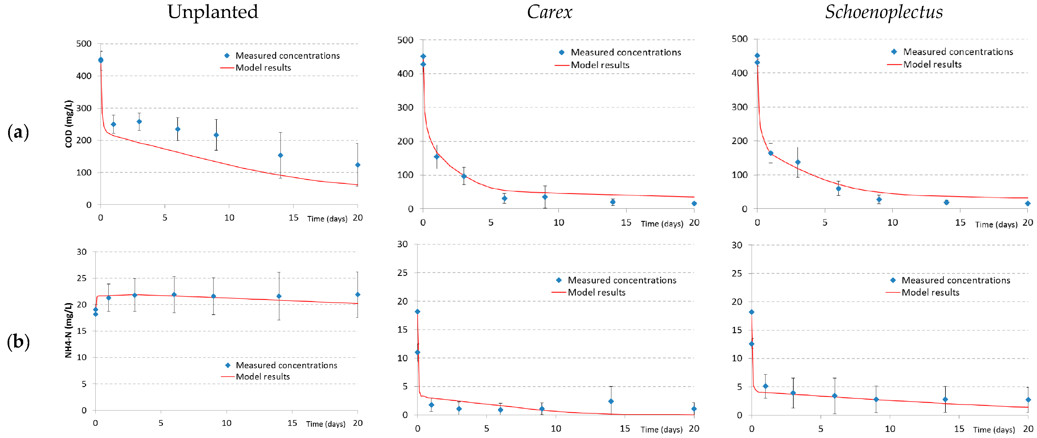
3.1. Simulation Results for Vertical Flow Wetlands Treating Domestic Wastewater

This section shows simulation results for VF wetlands using the HYDRUS Wetland Module. Simulations have been carried out for a VF pilot-scale wetland (Figure 1) operated in the technical laboratory hall of the Institute of Sanitary Engineering at BOKU University in Vienna, Austria [5]. The systems had a 60 cm main layer consisted of sand with a grain size of 0.06–4 mm (d10 = 0.2 mm; d60 = 0.8 mm) and a surface area of 1 m2. The intermediate layer (gravel 4–8 mm) prevents fine particles from being washed out into the drainage layer (gravel 16–32 mm). The systems were loaded four times per day with mechanically pre-treated municipal wastewater (each loading 10 L) and were planted with giant cane (Arundo donax).
For the numerical simulations, only the main layer was considered. The transport domain, i.e., a vertical cross-section of the main layer, was discretized into 11 columns and 40 rows. Using this discretisation, the two-dimensional finite element mesh consists of 440 nodes and 780 finite elements. An atmospheric boundary condition is assigned to the top of the system, a constant pressure head boundary condition with a constant head of −2 cm [5].
Table 3 shows three parameter sets of the van Genuchten–Mualem model [35] of the soil hydraulic properties used in simulations of water flow. The “HYDRUS parameter set forSand’” uses default soil hydraulic properties for sand provided by HYDRUS. For the “Measured Ks and porosity” parameter set, measured values of porosity and saturated hydraulic conductivity Ks were used whereas the default residual water content and shape parameters were used for sand. The third parameter set was obtained by inverse simulation. Measured effluent flow rates were used to estimate the soil hydraulic parameters (i.e., residual water content and shape parameters) using the inverse simulation routine provided by HYDRUS [13]. Measured values of porosity and Ks were kept constant. Figure 2 compares the measured and simulated effluent flow rates using these three parameter sets. The simulated effluent flow rate is rather constant when using the default parameter set for sand due to the low Ks value. When using the “Measured Ks and porosity” parameter set, measured and simulated effluent flow rates match better, however, the peak of the effluent flow rate is over-predicted and occurs too early. Using the “Fitted parameter set”, a good match between simulated and measured data can be achieved. The results show that by measuring the porosity and the saturated hydraulic conductivity of the filter material, the results can be greatly improved and thus these two parameters should be measured when modelling VF wetlands.
Table 4 shows measured and simulated concentrations of ammonia and nitrate nitrogen (NH4-N and NO3-N, respectively) for the VF pilot-scale wetlands with two different sandy filter materials used for the main layer. In addition to the sand with a grain size of 0.06–4 mm, in a parallel-operated VF wetland, sand with a grain size of 1–4 mm was also used. The different levels of the NO3-N effluent concentrations for the two filter materials could be simulated. For the VF wetland with 1–4 mm sand, the effluent concentrations of NO3-N have been higher. This can be explained by the fact that due to the higher flow rates, less readily degradable organic matter is produced by hydrolysis and thus denitrification is limited by lack of available organic matter [16].
For the VF pilot-scale wetlands with a main layer of 0.06–4 mm sand, the distribution of microbial and bacterial biomass in different depths of the filter was also measured [36]. Converting the measured data into biomass COD results in mean values of 3400 to 5100 μg·COD/g·DW (dry weight of the substrate, i.e., sand) for the first cm of the main layer, 1100 to 2600 μg·COD/g·DW from 1 to 5 cm, and 640 to 1400 μg·COD/g·DW from 5 to 10 cm, respectively. Most of the biomass could be found in the upper 10 cm of the VF bed [18].
When using heterotrophic lysis rates of between 0.25 and 0.35 day−1, the simulated microbial biomass COD is between 5600 and 3400 μg·COD/g·DW (the range of the measured values) in the first cm of the main layer. Calculated and simulated microbial biomass COD in different depths of the main layer showed a good fit for a heterotrophic lysis rate of 0.30 day−1 (Figure 3). When comparing measured and simulated biomass COD in different depths of the main layer, simulations seem to over-predict biomass COD in 1–5 cm depth and under-predict biomass COD in 5–10 cm depth. This could be an indication that the influence of biomass growth on the hydraulic properties has to be considered in the model [18].
Additionally, outdoor experiments have been carried out at experimental wetlands located at the wastewater treatment plant Ernsthofen, Lower Austria [38]. Three VF wetlands with a surface area of about 20 m2 each have been operated in parallel. The organic loading rates for bed 1 through 3 have been 20, 27 and 40 g·COD·m−2·day−1, which correspond to hydraulic loading rates of 32.2, 43.0, and 64.7 mm/day, respectively. The main layer of the filter consisted of 50 cm sandy substrate (gravel size 0.06–4 mm, d10 = 0.2 mm; d60 = 0.8 mm). All three VF wetlands have been planted with common reed (Phragmites australis). The data gained from this experiment have been used to verify the temperature model incorporated into CW2D [17].
The width of the transport domain in the numerical simulations was 4 m, and its depth 0.8 m, while the transport domain itself was discretized into 31 columns and 33 rows. The two-dimensional finite element mesh consisted of 1023 nodes and 1920 triangular finite elements. An atmospheric boundary condition was assigned to the top of the system representing the influent distribution system, and a constant pressure head boundary condition (constant head of −4 cm) was assigned to one side of the drainage layer [17].
Measured and simulated effluent flow rate and cumulative effluent of the experimental wetland showed good match [17]. Using the calibrated water flow model and using the original CW2D parameter set [14], measured effluent concentrations during summer could be simulated. However, at lower temperatures, measured COD and NH4-N effluent concentrations could not be simulated because hydrolysis and nitrification at low temperatures were over predicted. The standard CW2D parameter set considers temperature dependencies only for maximum growth, decay and hydrolysis rates. Using a modified parameter set (that includes temperature dependencies for the half-saturation constants of hydrolysis and nitrification) measured and simulated COD and NH4-N effluent concentrations showed a good fit (Figure 4). With this modified parameter set, simulating the COD and NH4-N effluent concentrations at low temperatures was possible [17]. Temperature dependencies for the half-saturation constants of hydrolysis and nitrification are now included in the standard parameter sets of CW2D and CWM1 [7].

3.2. Experiences and Challenges Using Process-Based Wetland Models

3.2.1. Water Flow Model

It is generally agreed that the hydraulics have a high impact on the treatment performance of TWs. When simulating SSF wetlands, the first step thus should be a good calibration of the water flow model. Experience shows that simulated effluent concentrations can match the measured data only when the hydraulic behaviour of the system is well described.
For VF wetlands, the influence of the parameters describing the hydraulic properties of the filter material (such as for the van Genuchten–Mualem model [35] in HYDRUS [13]) is much higher than the influence of the parameters of the biokinetic model [31]. To achieve a good calibration of the water flow model, it is advised to measure at least the porosity and the saturated hydraulic conductivity of the filter material and, if possible, the volumetric effluent flow rate between two intermittent loadings [3]. With these measurements, it is possible to estimate the remaining parameters describing the hydraulic properties of the filter material using the inverse simulation implemented in HYDRUS [13] (see also Figure 2).
Preferential flow paths in VF wetlands can be caused by macropores/cracks in some layers. Through this effect, water can bypass most of the soil porous matrix in an unpredictable way [39]. This is especially true for the sludge layer in French VF wetlands [40,41]. Water flow in such systems cannot be modelled with uniform flow models (such as using the Richards equation combined with the van Genuchten–Mualem function in HYDRUS [13]). A non-equilibrium approach uses a model that separately describes flow and transport in preferred flow paths and slow or stagnant pore regions. This approach seems to be more appropriate for simulating preferential flow in VF wetlands [39]. Such a dual-porosity model therefore also needs to be incorporated into the software tools to accurately describe water flow and solute transport in French VF wetlands.
For HF wetlands in which gravel is usually used as filter material, the saturated hydraulic conductivity of gravel is much larger than the actual water flow in the filter. Tracer experiments are usually applied to calibrate the water flow and single solute transport models.

3.2.2. Transport Model

Tracer experiments are used to calibrate the transport model, i.e., the transport of solutes through the filter bed of VF and HF wetlands. When calibrating tracer experiments, i.e., one tries to match measured and simulated breakthrough curves, the longitudinal dispersion coefficient is the most sensitive parameter and has the highest influence on the simulation results.
When simulating tracer breakthrough curves, the selection of the proper water flow model is important. If sand is used as filter media, single-porosity models such as the van Genuchten–Mualem model [35] are sufficient and measured breakthrough curves from tracer experiments can be fitted well [16,26]. However, if filter media with high porosity such as woodchips and/or crushed seashells are used [33], the use of dual-porosity models might be required (similar as for simulating preferential flow in the sludge layer of French VF wetlands). Dual-porosity models consider mobile and immobile water zones and exchange of solutes between these two phases. A number of dual-porosity models are implemented in the HYDRUS software package [13]. Currently, the use of the HYDRUS Wetland Module is limited to single-porosity models.
For a number of substances (e.g., ammonia, phosphate), adsorption/desorption is a main retention mechanism. It is advised to use measured adsorption isotherms for the filter material used. For some applications, adsorption also needs to be considered for some COD fractions, e.g., when simulating wetlands treating CSO [22]. Also, slow release of carbon from soils or specific filter media can be modelled by considering adsorption/desorption for different fractions of COD [32].

3.2.3. Biokinetic Model

Bacteria in TWs are similarly to those in activated sludge systems. Based on this assumption, it was proposed that parameters of the biokinetic models developed for activated sludge systems should be applicable to describe processes in TWs as well [42]. This assumption was confirmed by a number of applications of the HYDRUS Wetland Module that showed that a good match between measured and simulated concentrations could be achieved when the hydraulic behaviour of the system is well described (see above). Additionally, Table 5 shows good agreement between measured and calculated volumetric nitrification rates [43].
When using the biokinetic models, such as CW2D or CWM1, it is therefore advised not to change the default parameters of the biokinetic model, except for good reasons. However, parameters describing treated wastewater and that are related to the chosen biokinetic model have to be amended and shall be used for calibration process. Influent fractionation has high impact on the simulation results and needs to be adapted for each simulation study as treated wastewaters are different. Parameters describing the influent fractionation include (1) fractionation of influent COD (i.e., estimation of different COD model fractions from measured total COD) and (2) organic N content of different COD fractions.
Rizzo et al. [29] described the set-up of a model to simulate experimental data from a HF wetland fed with artificial wastewater. During the experiments, the only nitrogen parameter measured in influent was TKN (Total Kjehldal Nitrogen). As the model requires influent concentrations of ammonia nitrogen, the organic N content of different COD fractions had to be adapted from standard values for the type of used artificial wastewater. This results in different ratios of ammonia nitrogen to TKN. Figure 5 shows the impact of different influent concentrations of ammonia nitrogen on simulated effluent concentrations. When all influent TKN is assumed to be ammonia (i.e., no organic nitrogen is present), simulated effluent concentrations of ammonia nitrogen are higher than measured effluent concentrations. On the contrary, when all influent TKN is assumed to be organic nitrogen (i.e., no ammonia is present), simulated effluent concentrations are too low.
Pucher and Langergraber [44] simulated VF filters treating domestic wastewater. The main layer of two parallel operated filters consisted of sand with a grain size of 1–4 mm or zeolite with a grain size of 2–5 mm. Both filters had an impounded drainage layer. After calibrating the flow model for the sand and zeolite filters (Table 6), the procedure for calibrating the biokinetic model was as follows: the standard parameter set of the CW2D biokinetic model [7] was used in the first simulation of the sand filter (“Effluent (Sand)—Simulated 1” in Table 7). This resulted in over-prediction of nitrification, i.e., simulated ammonia nitrogen concentrations were much lower than measured data. After reducing the maximum nitrification rate from 0.9/day to 0.175/day, the simulated effluent concentrations of ammonia nitrogen matched measured data well (“Effluent (Sand)—Simulated 2” in Table 7). After adding the measured adsorption isotherms [45] and a first-order rate coefficient for non-equilibrium adsorption of 0.01/day in the zeolite filter simulation compared to the sand filter simulation, a good match between simulated and measured date could be obtained (“Effluent (Zeolite)—Simulated” in Table 7).
Pálfy and Langergraber [28] simulated experimental results from batch-fed column experiments using the CWM1 biokinetic model. They described the need to adjust some parameters of the biokinetic model, i.e., the inhibition coefficients of acetotrophic methanogenic and sulphate reducing bacteria for dissolved oxygen and nitrate, respectively, to be able to simulate anaerobic, anoxic, and aerobic processes to occur in parallel. The local effect of root zone re-aeration can explain these phenomena. Figure 6 shows measured and simulated sulphate concentrations before (a) and after (b) the adjustment of parameters of the CWM1 biokinetic model. Batch experiments can be used to calibrate the biokinetic model parameters, as there is no impact of water flow on the treatment performance.

3.2.4. Plant Model

It is generally agreed that plants play an indispensable factor in treatment wetlands. The plant model that can be used with the HYDRUS Wetland Module describes nutrient uptake coupled to water uptake (which is modelled by the evapotranspiration rate). This approach has been shown to be sufficient for high loaded systems; however, for water qualities with lower nutrient contents, the simulated potential nutrient uptake is far over-estimated [47].
Toscano et al. [26] simulated pilot-scale two-stage subsurface flow treatment wetlands in Eastern Sicily. HF and VF wetlands were used for secondary and tertiary treatment of municipal wastewater. Each of the wetland cells had a surface area of 4.5 m2 (1.5 m × 3.0 m). The HF beds were filled with 0.6 m volcanic gravel having a size of 10–15 mm. The VF beds were filled with two different filter media: volcanic sand as the main layer for a depth of 0.5 m (about 0.06–4 mm; d10 = 0.13 mm; d60 = 2.0 mm) at the top of the filter bed and coarse volcanic gravel as the drainage layer (about 16–32 mm, 25 cm depth). The average influent flow rate for each line was about 40 ± 5 L/h. Planted and unplanted VF and HF beds have been operated in parallel. Planted wetland cells were planted with reed (Phragmites sp.). For the simulations, an oxygen release of 5 g O2/m2/day and an evapotranspiration rate of 7.4 mm/day were used. Additionally, N and P uptake by plants was considered. Using these input data for the plant model, simulated effluent concentrations matched the measure concentrations well (Table 8). The effect of the plants can be best seen for the HF wetlands: the different NH4-N effluent concentrations in planted and unplanted HF wetlands could be simulated. In the model, the difference was caused by uptake of ammonia by wetland plants through their roots as well as ammonia removal through nitrification that was possible due to the oxygen input via the roots. The simulated NO3-N effluent concentrations are a clear indication of nitrification in the HF filter bed. For VF wetlands, no significant difference between planted and unplanted wetland cells was observed or simulated.
As described above, Pálfy and Langergraber [28] simulated batch-fed column experiments. Figure 7 shows the measured and simulated COD, NH4-N and SO4-S concentrations at 12 °C. The different behaviour of unplanted columns as well as those planted with Carex and Schoenoplectus could be simulated. Parameters of the biokinetic model were adjusted using the unplanted columns. For modelling the effect of the wetland plants, only the parameters’ oxygen release and evapotranspiration rate were adjusted. These experiments clearly showed that the different effects of wetland plants on the treatment performance of wetland systems can be modelled with existing plant models.

3.2.5. Clogging Model

Up to now, modelling of clogging processes is not possible using the HYDRUS Wetland Module. In a first trail, the colloids attachment/detachment model implemented in the HYDRUS C-Ride module [34,48] was coupled with the CW2D biokinetic model [49]. It was assumed that CS, the slowly biodegradable organic matter (as defined by [14]), consists of a particulate matter XS (slowly biodegradable organic matter as defined in the CWM1 biokinetic model [14]) that can be divided into five different classes according to different particle sizes (<1, 1–3, 3–10, 10–30, and 30–100 μm, respectively). It was further assumed that particles are transported in the liquid phase until they are attached. Once attached, the particles undergo hydrolysis and CR (readily biodegradable organic matter as defined in the CWM1 biokinetic model [14]) in the liquid phase that is produced. An additional assumption was that particles with different sizes have the same density and degradability.
The model was tested using measurements of particle concentrations in different depths of the 50-cm main layer of the VF pilot-scale wetland as described before. Particle measurements at the inlet were used to calculate fractionation of COD influent. Measured and simulated soluble particulate COD concentrations for the 10–30 μm particle class before and after loading of the VF wetland along the filter depth are shown in Figure 8. “Measured” particulate COD was calculated from particle measurements. In general, the first test showed a good agreement between measured and simulated particulate COD. However, there is still a great need for further testing of the particle transport model and for finding an optimal parameter set for various conditions present in treatment wetlands.
Several clogging models have been developed for BIO_PORE [7]. Samsó and García [50] described the relation between bacterial communities and accumulated solids, leading to clogging in a HF wetland. The so-called “Cartridge Theory” describes how the active bacterial zone moves in the filter. In this model, the effect of the inert organic matter accumulated in pores on the hydraulic conductivity is not considered. A description of limited growth of bacteria was implemented by adding two parameters. A negative feedback term is provided by the first parameter to prevent unlimited bacteria growth in areas where substrate concentrations are high (which is especially relevant for the influent zones of HF wetlands). The second parameter decreases the growth rate of bacteria when pore space is limited. Bacteria density and accumulated inert solids also had an effect on simulated effluent concentrations [50] and on effluent pollutant concentrations; again, only without considering the effect of organic matter accumulation on water flow. Additionally, the effect of a pore size reduction on the hydraulic conductivity is described using the biological clogging model proposed by Mostafa and Van Geel [51]. Using this approach, a realistic behaviour of HF wetlands, including overland flow and re-infiltration of water in the unused filter material could be simulated [52,53]. In the work of Rajabzadeh et al. [54], a computational fluid dynamics model was used to simulate biofilm development and the effect on local porosity in a saturated vertical downflow wetland. There was good agreement between simulation results and measured data for predicting clogging due to biomass growth were good [54].

3.2.6. Wetland Models as Design Tools

Further developments of existing models are needed to make them a useful and applicable tool for a TW design [3]. A simplified computer-based TW design tool, based on process-based numerical models, should be developed that
  • could be used when having knowledge about a TW design, but without requiring special knowledge about numerical modelling,
  • allows the design of TWs for different boundary conditions (such as different climatic conditions, wastewater characterization, filter material, etc.), and
  • makes the description of the dynamic behaviour of the designed TW possible, thus allowing the higher robustness of wetland treatment systems, for example, for fluctuating inflows and peak loads.
Several developments have been made to develop such a simplified design tool. RSF_Sim [55] supports the design of wetlands for a combined sewer overflow treatment (in Germany named retention soil filters, i.e., RSFs). This simplified, yet robust and reliable, model was developed for design purposes based on experiences with the HYDRUS Wetland module. Only few parameters are required in RSF_Sim which makes it very simple to use. RSF_Sim was developed specifically for German conditions. RSF_Sim was also adapted for a combined sewer overflow treatment for French conditions considering e.g., different design rules and effluent requirements [56,57].
A similar approach was taken for developing a simple model to support the design of French VF wetlands [58]. Numerical simulations using the HYDRUS Wetland Module were first performed, varying a number of design parameters. The design parameters included the depth of the main layer of the first stage filter, the hydraulic loading rate, and the inlet COD concentration and temperature. Effluent concentrations of the first stage filter were then verified using measured data and a surrogate model was developed to estimate COD and NH4-N removal in relation to the design parameters. Although the first results were promising, it was concluded that more work needs to be done to develop a robust design model [58].

4. Conclusions

Interest in modelling processes occurring in treatment wetlands has increased over the last 15 years. Several mechanistic models to describe processes in subsurface flow treatment wetlands have been developed. The HYDRUS Wetland Module, up to now, is the only one that is commercially available and thus available for wider use.
Experiences with applying the HYDRUS Wetland Module and other existing simulation tools can be summarised as follows:
  • Process-based models are a powerful tool for understanding the processes in treatment wetlands in more detail.
  • All sub-models required to describe the different processes in treatment wetlands are important.
    Good calibration of the water flow model is a pre-requisite for achieving a good match between measured and simulated pollutant concentrations. Due to the intermittent loading, more data are required for VF wetlands compared to HF wetlands. If the water flow model is calibrated, good results can be obtained in most applications when using the standard parameter sets of the biokinetic CW2D and CWM1 biokinetic models [7].
    A good description of solute transport in the porous media is of equal importance for good simulation results for pollutant degradation and removal. To be able to model realistic solute transport behaviour, it is advised to carry tracer experiments. Adsorption and desorption is an important process for several parameters (such as ammonia and phosphate), especially when reactive filter media are used.
    Influent fractionation (i.e., fractionation of influent COD and the N and P contents of different COD fractions) has a high impact on simulation results and thus is an essential part of calibrating reactive transport models. This is especially true when simulating wetlands treating other than domestic wastewater. Parameters of the biokinetic model should be changed only after a good calibration of the water flow and transport models has been achieved and after the effect of the influent fractionation on simulation results has been considered.
    Simulating the influence of wetland plants is possible by considering uptake and release via the plant roots linked to evapotranspiration. Modelling the effect of plants on the treatment performance has been shown to be most important for HF wetland and batch-operated systems and less important for VF wetlands.
    Models describing clogging are important to describe the long-term behaviour of treatment wetlands. Up to now, clogging models are the least established and tested among the sub-models mentioned. Further research is needed to get better reliability in clogging model predictions.
  • One of the main obstacles for the wider use of available simulation tools is that they are rather complicated and difficult to run. Simplified, yet robust and reliable models for the design of treatment wetlands, need to be developed (such as RSF_Sim, developed to support the design of treatment wetlands treating combined sewer overflow [55]).

Conflicts of Interest

The author declares no conflict of interest.

References

  1. Kadlec, R.H.; Wallace, S. Treatment Wetlands, 2nd ed.; CRC Press: Boca Raton, FL, USA, 2009. [Google Scholar]
  2. García, J.; Rousseau, D.P.L.; Morató, J.; Lesage, E.; Matamoros, V.; Bayona, J.M. Contaminant Removal Processes in Subsurface-Flow Constructed Wetlands: A Review. Crit. Rev. Environ. Sci. Technol. 2010, 40, 561–661. [Google Scholar] [CrossRef]
  3. Langergraber, G. Numerical modelling: A tool for better constructed wetland design? Water Sci. Technol. 2011, 64, 14–21. [Google Scholar] [CrossRef] [PubMed]
  4. Langergraber, G.; Rousseau, D.; García, J.; Mena, J. CWM1—A general model to describe biokinetic processes in subsurface flow constructed wetlands. Water Sci. Technol. 2009, 59, 1687–1697. [Google Scholar] [CrossRef] [PubMed]
  5. Langergraber, G. Modeling of processes in subsurface flow constructed wetlands—A review. Vadose Zone J. 2008, 7, 830–842. [Google Scholar] [CrossRef]
  6. Langergraber, G.; Morvannou, A. Modelling of Treatment Wetlands. Sustain. Sanit. Pract. 2014, 18, 31–36. [Google Scholar]
  7. Langergraber, G.; Šimůnek, J. Reactive Transport Modeling of Subsurface Flow Constructed Wetlands Using the HYDRUS Wetland Module. Vadose Zone J. 2012, 11, 460. [Google Scholar] [CrossRef]
  8. Samsó, R.; Garcia, J. BIO PORE, a mathematical model to simulate biofilm growth and water quality improvement in porous media: Application and calibration for constructed wetlands. Ecol. Eng. 2013, 54, 116–127. [Google Scholar] [CrossRef]
  9. Langergraber, G.; Giraldi, D.; Mena, J.; Meyer, D.; Peña, M.; Toscano, A.; Brovelli, A.; Korkusuz, E.A. Recent developments in numerical modelling of subsurface flow constructed wetlands. Sci. Total Environ. 2009, 407, 3931–3943. [Google Scholar] [CrossRef] [PubMed]
  10. Kumar, J.L.G.; Zhao, Y.Q. A review on numerous modeling approaches for effective, economical and ecological treatment wetlands. J. Environ. Manag. 2011, 92, 400–406. [Google Scholar] [CrossRef] [PubMed]
  11. Meyer, D.; Chazarenc, F.; Claveau-Mallet, D.; Dittmer, U.; Forquet, N.; Molle, P.; Morvannou, A.; Pálfy, T.; Petitjean, A.; Rizzo, A.; et al. Modelling constructed wetlands: Scopes and aims—A comparative review. Ecol. Eng. 2015, 80, 205–213. [Google Scholar] [CrossRef]
  12. Samsó, R.; Meyer, D.; García, J. Subsurface Flow Constructed Wetland Models: Review and Prospects. In The Role of Natural and Constructed Wetlands in Nutrient Cycling and Retention on the Landscape; Vymazal, J., Ed.; Springer: Cham, Switzerland, 2015; pp. 149–174. [Google Scholar]
  13. Šimůnek, J.; Šejna, M.; van Genuchten, M.T. The HYDRUS Software Package for Simulating the Two- and Three-Dimensional Movement of Water, Heat, and Multiple Solutes in Variably-Saturated Media. In Technical Manual, version 2.0; PC-Progress: Prague, Czech Republic, 2011; p. 254. [Google Scholar]
  14. Langergraber, G.; Šimůnek, J. Modeling variably-saturated water flow and multi-component reactive transport in constructed wetlands. Vadose Zone J. 2005, 4, 924–938. [Google Scholar] [CrossRef]
  15. Šimůnek, J.; van Genuchten, M.T.; Šejna, M. Development and applications of the HYDRUS and STANMOD software packages and related codes. Vadose Zone J. 2008, 7, 587–600. [Google Scholar] [CrossRef]
  16. Langergraber, G. Simulation of subsurface flow constructed wetlands—Results and further research needs. Water Sci. Technol. 2003, 48, 157–166. [Google Scholar] [PubMed]
  17. Langergraber, G. Simulation of the treatment performance of outdoor subsurface flow constructed wetlands in temperate climates. Sci. Total Environ. 2007, 380, 210–219. [Google Scholar] [CrossRef] [PubMed]
  18. Langergraber, G.; Tietz, A.; Haberl, R. Comparison of measured and simulated distribution of microbial biomass in subsurface vertical flow constructed wetlands. Water Sci. Technol. 2007, 56, 233–240. [Google Scholar] [CrossRef] [PubMed]
  19. Hochfeldt, V. Numerical Simulation of a Full-Scale Two-Stage Constructed Wetland System. Master’s Thesis, University of Applied Sciences Ostwestfahlen-Lippe, Höxter, Germany, 2016. [Google Scholar]
  20. Pucher, B.; Ruiz, H.; Paing, J.; Chazarenc, F.; Molle, P.; Langergraber, G. Using simulation of a one stage vertical flow constructed wetland to determine filter depth of a zeolite layer to improve the treatment performance. Water Sci. Technol. 2016. submitted. [Google Scholar]
  21. Dittmer, U.; Meyer, D.; Langergraber, G. Simulation of a Subsurface Vertical Flow Constructed Wetland for CSO Treatment. Water Sci. Technol. 2005, 51, 225–232. [Google Scholar] [PubMed]
  22. Henrichs, M.; Langergraber, G.; Uhl, M. Modelling of organic matter degradation in constructed wetlands for treatment of combined sewer overflow. Sci. Total Environ. 2007, 380, 196–209. [Google Scholar] [CrossRef] [PubMed]
  23. Henrichs, M.; Welker, A.; Uhl, M. Modelling of biofilters for ammonium reduction in combined sewer overflow. Water Sci. Technol. 2009, 60, 825–831. [Google Scholar] [CrossRef] [PubMed]
  24. Meyer, D. Modellierung und Simulation von Retentionsbodenfiltern zur weitergehenden Mischwasserbehandlung (Modelling and Simulation of Constructed Wetlands for Treatment of Combined Sewer Overflow). Ph.D. Thesis, Technical University of Kaiserslautern, Kaiserslautern, Germany, 2011. Available online: https://kluedo.ub.uni-kl.de/frontdoor/index/index/docId/2843 (accessed on 14 August 2013). [Google Scholar]
  25. Pálfy, T.G.; Molle, P.; Langergraber, G.; Meyer, D. Simulation of constructed wetlands treating combined sewer overflow using HYDRUS/CW2D. Ecol. Eng. 2016, 87, 340–347. [Google Scholar] [CrossRef]
  26. Toscano, A.; Langergraber, G.; Consoli, S.; Cirelli, G.L. Modelling pollutant removal in a pilot-scale two-stage subsurface flow constructed wetlands. Ecol. Eng. 2009, 35, 281–289. [Google Scholar] [CrossRef]
  27. Pálfy, T.G.; Gribovszki, Z.; Langergraber, G. Design-support and performance estimation using HYDRUS/CW2D: A horizontal flow constructed wetland for polishing SBR effluent. Water Sci. Technol. 2015, 71, 965–970. [Google Scholar] [CrossRef] [PubMed]
  28. Pálfy, T.G.; Langergraber, G. The verification of the Constructed Wetland Model No.1 implementation in HYDRUS using column experiment data. Ecol. Eng. 2014, 68, 105–115. [Google Scholar] [CrossRef]
  29. Rizzo, A.; Langergraber, G.; Galváo, A.; Boano, F.; Revelli, R.; Ridolfi, L. Modelling the response of horizontal flow constructed wetlands to unsteady organic loads with HYDRUS-CWM1. Ecol. Eng. 2014, 68, 209–213. [Google Scholar] [CrossRef]
  30. Rizzo, A.; Langergraber, G. Novel insights on the response of horizontal flow constructed wetland to sudden changes in influent loads from a modelling investigation. Ecol. Eng. 2016, 93, 242–249. [Google Scholar] [CrossRef]
  31. Karlsson, S.C.; Langergraber, G.; Pell, M.; Dalahmeh, S.; Vinnerås, B.; Jönsson, H. Simulation and verification of hydraulic properties and organic matter degradation in sand filters for greywater treatment. Water Sci. Technol. 2015, 71, 426–433. [Google Scholar] [CrossRef] [PubMed]
  32. Smethurst, P.J.; Petrone, K.; Langergraber, G.; Baillie, C.; Worledge, D. Nitrate dynamics in a rural headwater catchment: Measurements and modeling. Hydrol. Process. 2014, 28, 1820–1834. [Google Scholar] [CrossRef]
  33. Pugliese, L.; Bruun, J.; Kjaergaard, C.; Hoffmann, C.C.; Langergraber, G. Nonequilibrium model for solute transport in full size subsurface flow constructed wetland. Ecol. Eng. 2016. submitted. [Google Scholar]
  34. Šimůnek, J.; Jacques, D.; Langergraber, G.; Bradford, S.A.; Šejna, M.; van Genuchten, M.T. Numerical Modeling of Contaminant Transport Using HYDRUS and its Specialized Modules. J. Indian Inst. Sci. 2013, 93, 265–284. [Google Scholar]
  35. Van Genuchten, M.T. A closed form equation for predicting the hydraulic conductivity of unsaturated soils. Soil Sci. Soc. Am. J. 1980, 44, 892–898. [Google Scholar] [CrossRef]
  36. Tietz, A.; Langergraber, G.; Sleytr, K.; Kirschner, A.; Haberl, R. Characterization of microbial biocoenosis in vertical subsurface flow constructed wetlands. Sci. Total Environ. 2007, 380, 163–172. [Google Scholar] [CrossRef] [PubMed]
  37. Langergraber, G. Erratum: Water Science and Technology 56, 2007, 233–240: Comparison of measured and simulated distribution of microbial biomass in subsurface vertical flow constructed wetlands. Water Sci. Technol. 2015, 71, 157–158. [Google Scholar] [CrossRef] [PubMed]
  38. Langergraber, G.; Prandtstetten, C.; Pressl, A.; Haberl, R.; Rohrhofer, R. Removal efficiency of subsurface vertical flow constructed wetlands for different organic loads. Water Sci. Technol. 2007, 56, 75–84. [Google Scholar] [CrossRef] [PubMed]
  39. Morvannou, A.; Forquet, N.; Vanclooster, M.; Molle, P. Which hydraulic model to use in vertical flow constructed wetlands? In Proceedings of the 13th IWA Specialized Group Conference on “Wetland Systems for Water Pollution Control”, Perth, Australia, 25–29 November 2012; Conference Papers Volume 2. Dallas, S., Ed.; Murdoch University: Perth, Australia, 2012; pp. 145–153. [Google Scholar]
  40. Molle, P.; Liénard, A.; Boutin, C.; Merlin, G.; Iwema, A. How to treat raw sewage with constructed wetlands: An overview of the French systems. Water Sci. Technol. 2005, 51, 11–21. [Google Scholar] [PubMed]
  41. Troesch, S.; Esser, D. Constructed Wetlands for the Treatment of Raw Wastewater: The French Experience. Sustain. Sanit. Pract. 2012, 12, 9–15. [Google Scholar] [CrossRef]
  42. Langergraber, G. Development of a Simulation Tool for Subsurface Flow Constructed Wetlands. Ph.D. Dissertation, BOKU University, Vienna, Austria, 2001. [Google Scholar]
  43. Morvannou, A.; Choubert, J.-M.; Vanclooster, M.; Molle, P. Solid respirometry to characterize nitrification kinetics: A better insight for modelling nitrogen conversion in vertical flow constructed wetlands. Water Res. 2011, 45, 4995–5004. [Google Scholar] [CrossRef] [PubMed]
  44. Puchner, B.; Langergraber, G. Simulation of two-stage vertical flow sand and zeolite filters treating domestic wastewater using the HYDRUS wetland module. In Proceedings of the 6th International Symposium on “Wetland Pollution Dynamics and Control” and Annual Conference of the Constructed Wetland Association, York, UK, 13–18 September 2015; Dotro, G., Gagnon, V., Eds.; Book of Abstracts. Cranfield University: Cranfield, UK, 2015; pp. 198–199. [Google Scholar]
  45. Dal Santo, S.; Canga, E.; Pressl, A.; Borin, M.; Langergraber, G. Investigation of nitrogen removal in a two-stage subsurface vertical flow constructed wetland system using natural zeolite. In Proceedings of the 12th IWA Specialized Group Conference on “Wetland Systems for Water Pollution Control”, San Servolo, Venice, Italy, 3–8 October 2010; Masi, F., Nivala, J., Eds.; IRIDRA Srl: Florence, Italy, 2010; pp. 263–270. [Google Scholar]
  46. Pálfy, T. Verification of the Implementation of CWM1 in the HYDRUS Wetland Module. Master’s Thesis, BOKU University, Vienna, Austria, 2013. [Google Scholar]
  47. Langergraber, G. The role of plant uptake on the removal of organic matter and nutrients in subsurface flow constructed wetlands—A simulation study. Water Sci. Technol. 2005, 51, 213–223. [Google Scholar] [PubMed]
  48. Bradford, S.A.; Šimůnek, J.; Bettahar, M.; van Genuchten, M.T.; Yates, S.R. Modeling Colloid Attachment, Straining, and Exclusion in Saturated Porous Media. Environ. Sci. Technol. 2003, 37, 2242–2250. [Google Scholar] [CrossRef] [PubMed]
  49. Langergraber, G.; Šimůnek, J. Simulating particle transport in subsurface flow constructed wetlands with CW2D/HYDRUS. In Proceedings of the 3rd International Symposium on “Wetland Pollutant Dynamics and Control—WETPOL 2009”, Barcelona, Spain, 20–24 September 2009; Bayona, J.M., García, J., Eds.; Book of Abstracts. Universitat Politècnica de Catalunya: Barcelna, Spain, 2009; pp. 135–136. [Google Scholar]
  50. Samsó, R.; García, J. The Cartridge Theory: A description of the functioning of horizontal subsurface flow constructed wetlands for wastewater treatment, based on modelling results. Sci. Total Environ. 2014, 473–474, 651–658. [Google Scholar] [CrossRef] [PubMed]
  51. Mostafa, M.; Van Geel, P.J. Conceptual models and simulations for biological clogging in unsaturated soils. Vadose Zone J. 2007, 6, 175–185. [Google Scholar] [CrossRef]
  52. Samsó, R.; Blázquez, J.; Agulló, N.; Grau, J.; Torres, R.; García, J. Effect of bacteria density and accumulated inert solids on the effluent pollutant concentrations predicted by the constructed wetlands model BIO_PORE. Ecol. Eng. 2015, 80, 172–180. [Google Scholar] [CrossRef] [Green Version]
  53. Samsó, R.; García, J.; Molle, P.; Forquet, N. Modelling bioclogging in variably saturated porous media and the interactions between surface/subsurface flows: Application to Constructed Wetlands. J. Environ. Manag. 2015, 165, 271–279. [Google Scholar] [CrossRef] [PubMed]
  54. Rajabzadeh, A.R.; Legge, R.L.; Weber, K.P. Multiphysics modelling of flow dynamics, biofilm development and wastewater treatment in a subsurface vertical flow constructed wetland mesocosms. Ecol. Eng. 2014, 74, 107–116. [Google Scholar] [CrossRef]
  55. Meyer, D.; Dittmer, U. RSF_Sim—A simulation tool to support the design of constructed wetlands for combined sewer overflow treatment. Ecol. Eng. 2015, 80, 198–204. [Google Scholar] [CrossRef]
  56. Pálfy, T.G.; Meyer, D.; Molle, P. Orage: Simulation of planted detentive filters treating urban storm water. In Proceedings of the 6th International Symposium on Wetland Pollution Dynamics and Annual Conference of the Constructed Wetland Association, York, UK, 13–18 September 2015; Dotro, G., Gagnon, V., Eds.; Book of Abstracts. Cranfield University: Cranfield, UK, 2015; pp. 216–217. [Google Scholar]
  57. Pálfy, T.G.; Gourdon, R.; Meyer, D.; Troesch, S.; Molle, P. A dynamic design tool for CWs treating combined sewer overflow. In Proceedings of the 15th IWA Specialized Group Conference on “Wetland systems for Water Pollution Control”, Gdansk, Poland, 4–9 September 2016; Gajewska, M., Matej-Lukowicz, K., Wojciechowska, E., Eds.; Conference Proceedings Volume 2. Gdańsk University of Technology: Gdańsk, Poland, 2016; pp. 771–790. [Google Scholar]
  58. Morvannou, A.; Froquet, N.; Troesch, S.; Molle, P. Impact of design and operating conditions on vertical flow constructed wetland performances: Modelling and global assessment confrontation. In Proceedings of the 6th International Symposium on Wetland Pollution Dynamics and Annual Conference of the Constructed Wetland Association, York, UK, 13–18 September 2015; Dotro, G., Gagnon, V., Eds.; Book of Abstracts. Cranfield University: Cranfield, UK, 2015; pp. 196–197. [Google Scholar]
Figure 1. Schematic representation of the indoor VF pilot-scale wetland (values are in cm).
Water 09 00005 g001
Figure 2. Measured and simulated effluent flow rates of the VF pilot-scale wetland for a single loading of 10 L (“HYDRUS parameter set orSand’”, “Measured Ks and porosity” and “Fitted parameter set” represent the parameter sets from Table 3).
Water 09 00005 g002
Figure 3. Calculated and simulated microbial biomass COD (Chemical Oxygen Demand) in different depths of the main layer of the VF pilot-scale wetland (adapted from [18,37]).
Water 09 00005 g003
Figure 4. Measured and simulated COD and NH4-N effluent concentrations of the experimental VF wetland in Ernsthofen using the modified parameter set (adapted from [17]).
Water 09 00005 g004
Figure 5. Influence of inflow NH4-N concentrations on effluent NH4-N concentrations of a HF wetland (adapted from [6]).
Water 09 00005 g005
Figure 6. Measured and simulated sulphate concentrations for a batch-fed column at 24 °C planted with Carex spp. ((a): with a standard parameter set of the CWM1 biokinetic model; (b): after adjusting CWM1 biokinetic model parameters; adapted from [46]).
Water 09 00005 g006
Figure 7. Simulation results for COD (a) NH4-N (b) and SO4-S (c) at 12 °C for unplanned columns, and columns planted with Carex and Schoenoplectus. Continuous line: simulation results, dots: measurement means, intervals: standard deviation (adapted from [28]).
Water 09 00005 g007aWater 09 00005 g007b
Figure 8. Comparison of measured and simulated particulate COD for the 10–30 μm particle class (adapted from [49]).
Water 09 00005 g008
Table 1. Processes and components (a number of components/processes in brackets) and applications of the biokinetic models CW2D (Constructed Wetland 2D) and CWM1 (Constructed Wetland Model #1) [7].
Biokinetic ModelCW2DCWM1
ProcessesAerobic and anoxic (9 processes)Aerobic, anoxic, and anaerobic (17 processes)
ComponentsOxygen, organic matter, nitrogen, and phosphorus (12 components)Oxygen, organic matter, nitrogen, and sulphur (16 components)
ApplicationVertical flow (VF) wetlandsVF and HF wetlands
Lightly loaded horizontal flow (HF) wetlands
Table 2. Comparison of implemented sub-models in the HYDRUS Wetland Module and BIO_PORE (adapted from [6]).
Simulation ToolHYDRUS Wetland Module [7]BIO_PORE [8]
Flow modelRichards equation (variably saturated flow)Variable water table (saturated flow)
Transport modelAdvection, dispersion, adsorptionAdvection, dispersion, adsorption
Biokinetic modelCW2D + CWM1CWM1
Influence of plantsEvapotranspiration, uptake and release of substancesEvapotranspiration, uptake and release of substances
Clogging modelNot consideredIncluded
Table 3. Soil hydraulic parameters of the van Genuchten–Mualem model [35] for the 0.06–4 mm main layer.
ParameterResidual Water Content θrSaturated Water Content θsShape ParametersSaturated Hydraulic Conductivity Ks
αNL
Unit(-)(-)(1/cm)(-)(-)(cm/h)
HYDRUS parameter set for ‘Sand’0.0450.430.1452.680.529.7
Measured Ks and porosity0.0450.300.1452.680.5117
Fitted parameter set0.0130.300.1472.420.636117
Table 4. Median values of measured and simulated influent and effluent concentrations for NH4-N and NO3-N in mg/L (adapted from [16]).
ParameterInfluentEffluent (0.06–4 mm Sand)Effluent (1–4 mm Sand)
MeasuredMeasuredSimulatedMeasuredSimulated
NH4-N60.00.150.011.200.16
NO3-N3.038.541.150.063.0
Table 5. Comparison of measured and calculated volumetric nitrification rates (adapted from [43], SD = standard deviation).
MethodMeasured with Solid RespirometryCalculated from Simulation Results *
Results (mg·O2/Lsample/h)32–50 (mean = 41, SD = 9; 2 values)30.5
Notes: * From simulations using parameters for the biokinetic model from activated sludge systems.
Table 6. Estimated soil hydraulic parameters of the van Genuchten–Mualem model [35].
ParameterResidual Water Content θrSaturated Water Content θsShape ParametersSaturated Hydraulic Conductivity Ks
αNL
Unit(-)(-)(1/cm)(-)(-)(cm/min)
Sand (1–4 mm)0.0630.370.1243.20.4955
Zeolite (2–5 mm)0.0450.420.0964.61.27154
Table 7. Measured and simulated influent and effluent concentrations of VF filters (in mg/L, measured data: average values and standard deviations in brackets, simulated data: average values over 1 day; CR = readily biodegradable COD, CS = slowly biodegradable COD, and CI = inert COD as defined in the CW2D biokinetic model [7]; bold data are used for comparison).
Parameter CRCSCICODNH4-NNO2-NNO3-N
InfluentMeasured---294930.0080.59
Simulated27410020-930.0080.59
Effluent (Sand)Measured---35 (5)14.5 (4.6)0.026 (0.040)70.8 (8.4)
Simulated 10.170.0831.231.50.42<0.00385.7
Simulated 20.140.0129.430.015.30.01676.2
Effluent (Zeolite)Measured---29 (9)0.06 (0.05)0.52 (1.10)51.8 (4.6)
Simulated0.160.0129.129.30.27<0.00343
Table 8. Measured and simulated influent and effluent concentrations of planted and unplanted VF and HF wetlands for secondary treatment of municipal wastewater (in mg/L, standard deviations in brackets, adapted from [26]).
Parameter CODNH4-NNO2-NNO3-N
InfluentMeasured63.9 (3.3)22.1 (1.9)0.18 (0.38)0.34 (0.10)
Effluent HF (planted)Measured47.5 (2.8)16.6 (1.2)0.06 (0.05)0.18 (0.17)
Simulated44.417.20.022.82
Effluent HF (unplanted)Measured48.2 (4.1)20.4 (0.6)0.02 (0.01)0.12 (0.11)
Simulated50.621.56 × 10−51 × 10−4
Effluent VF (planted)Measured23.0 (2.5)2.0 (0.1)0.10 (0.07)16.2 (1.1)
Simulated24.60.540.0126.9
Effluent VF (unplanted)Measured23.2 (2.3)2.0 (0.1)0.19 (0.08)16.4 (1.3)
Simulated24.00.960.0125.0

