Article

The Impact of Para Rubber Expansion on Streamflow and Other Water Balance Components of the Nam Loei River Basin, Thailand

1
Department of Water Resources Engineering, Faculty of Engineer, Kasetsart University, Ngam Wong Wan Rd., Lat Yao, Chatuchak, Bangkok 10900, Thailand
2
Forestry Research Center, Faculty of Forestry, Kasetsart University, Bangkok 10900, Thailand
3
Land Development Department, Chatuchak, Bangkok 10900, Thailand
4
Center for Agricultural and Rural Development, Iowa State University, Ames, IA 50011-1054, USA
*
Author to whom correspondence should be addressed.
Water 2017, 9(1), 1; https://doi.org/10.3390/w9010001
Submission received: 15 October 2016 / Revised: 5 December 2016 / Accepted: 14 December 2016 / Published: 22 December 2016

Abstract

:
At present, Para rubber is an economical crop which provides a high priced product and is in demand by global markets. Consequently, the government of Thailand is promoting the expansion of Para rubber plantations throughout the country. Traditionally, Para rubber was planted and grown only in the southern areas of the country. However, due to the Government’s support and promotion as well as economic reasons, the expansion of Para rubber plantations in the northeast has increased rapidly. This support has occurred without accounting for suitable cultivation of Para rubber conditions, particularly in areas with steep slopes and other factors which have significant impacts on hydrology and water quality. This study presents the impacts of Para rubber expansion by applying the Soil and Water Assessment Tool (SWAT) hydrological model on the hydrology and water balance of the Nam Loei River Basin, Loei Province. The results showed that the displacement of original local field crops and disturbed forest land by Para rubber production resulted in an overall increase of evapotranspiration (ET) of roughly 3%. The major factors are the rubber canopy and precipitation. Moreover, the water balance results showed an annual reduction of about 3% in the basin average water yield, especially during the dry season.

1. Introduction

Zeigler et al. [1] estimated that over 500,000 ha of upland areas in southeast Asia had been converted to Para rubber (Heveabrasiliensis) production in southeast Asia by 2009 and that the land area devoted in the region to Para rubber production could double or triple by the year 2050 [1]. Updated estimates for the same timeframe indicate that the expansion of total rubber production area in non-traditional Southeast Asia growing regions at >1,000,000 ha and that the production area could increase by a factor of four by 2050 [2]. Much of the expansion is occurring in “marginal areas” that are vulnerable to increased soil erosion and other environmental problems [3].
Para rubber has become one of the most important economic crops in Thailand, which is now the largest exporter of Para rubber by volume worldwide [4]. Para rubber production started in southern Thailand over a century ago [5] and has expanded greatly in that region since then due to favorable climatic conditions and land types. However, the government of Thailand has implemented policies to promote the expansion of Para rubber plantations throughout other areas of the country. Due to the Government’s support and promotion as well as for economic reasons, the expansion of Para rubber plantations in the northeast has increased dramatically during the past decade. Continuing attractive prices have resulted in particularly rapid expansion of Para rubber plantations during the past few years, resulting an increase of nearly 500,000 ha (246,340 ha to 739,190 ha) between 2006 and 2015 [6,7,8,9], confirming earlier projections of greatly expanded production [1]. The government support of Para rubber production in the northeast has occurred without adequate investigation of suitable cultivation conditions. This has resulted in Para rubber production occurring in areas with steep slopes, non-ideal climatic conditions, and other factors which have resulted in significant negative impacts on regional hydrology and water quality.
The northeastern region of Thailand consists of 20 provinces which cover a total area of about 170,226 km2 or one-third of the country (Figure 1). Forest areas in the region are rapidly becoming degraded due to destruction of existing forest stands. This is occurring because of increased agricultural and Para rubber production to support the rapidly growing population, and burning during the summer to support wild game hunting. At present, the most extreme burning of forests in the country is occurring in north and northeast Thailand [10].
The northeastern region of Thailand (Figure 1) has a total agricultural area of 15.90 million ha, of which 6.65 million ha are suitable for rubber plantations [11]. To date, only a small portion of this potential area has been developed for Para rubber production although projections indicate greatly expanded production in the future. Investigations are urgently needed to determine how expanded rubber production in the northeast will impact environmental conditions in the region, especially rainwater, humidity, soil characteristics, hydrologic balance, flow regime and rock formation. Changes in soil quality can have a strong effect on the amount of drainable water, as well as physical, chemical and biological properties [12]. Decision-makers and planners face difficult challenges in meeting water conservation objectives, and managing the engineering, socioeconomic and environmental aspects of development and planning, related to Para rubber production in northeast Thailand. This is especially true in certain sub regions such as the Nam Loei River Basin (NLRB) in Loei province (Figure 1), where Para rubber production increased from 0.4% to 21.5% of the total land use between 2002 and 2015, resulting in an extremely volatile situation that is impacting the entire watershed. Hence, technical tools including the Soil and Water Assessment Tool (SWAT) watershed-scale water quality model [13,14,15,16] are needed to support in-depth hydrologic and environmental assessments of Para rubber production in the region. SWAT has been extensively tested for a wide range of environmental conditions and watershed scales [17,18,19,20] and has been used effectively in a number of land use change studies [21,22,23,24,25,26,27,28,29,30]. Thus, the specific objectives of this research are to: (1) report the hydrologic impacts of the increased Para rubber production in the NRLB that occurred during 2002 to 2009, and 2009 to 2015; and (2) identification of inappropriate areas for rubber plantation and risks of landslide.

2. Materials and Methods

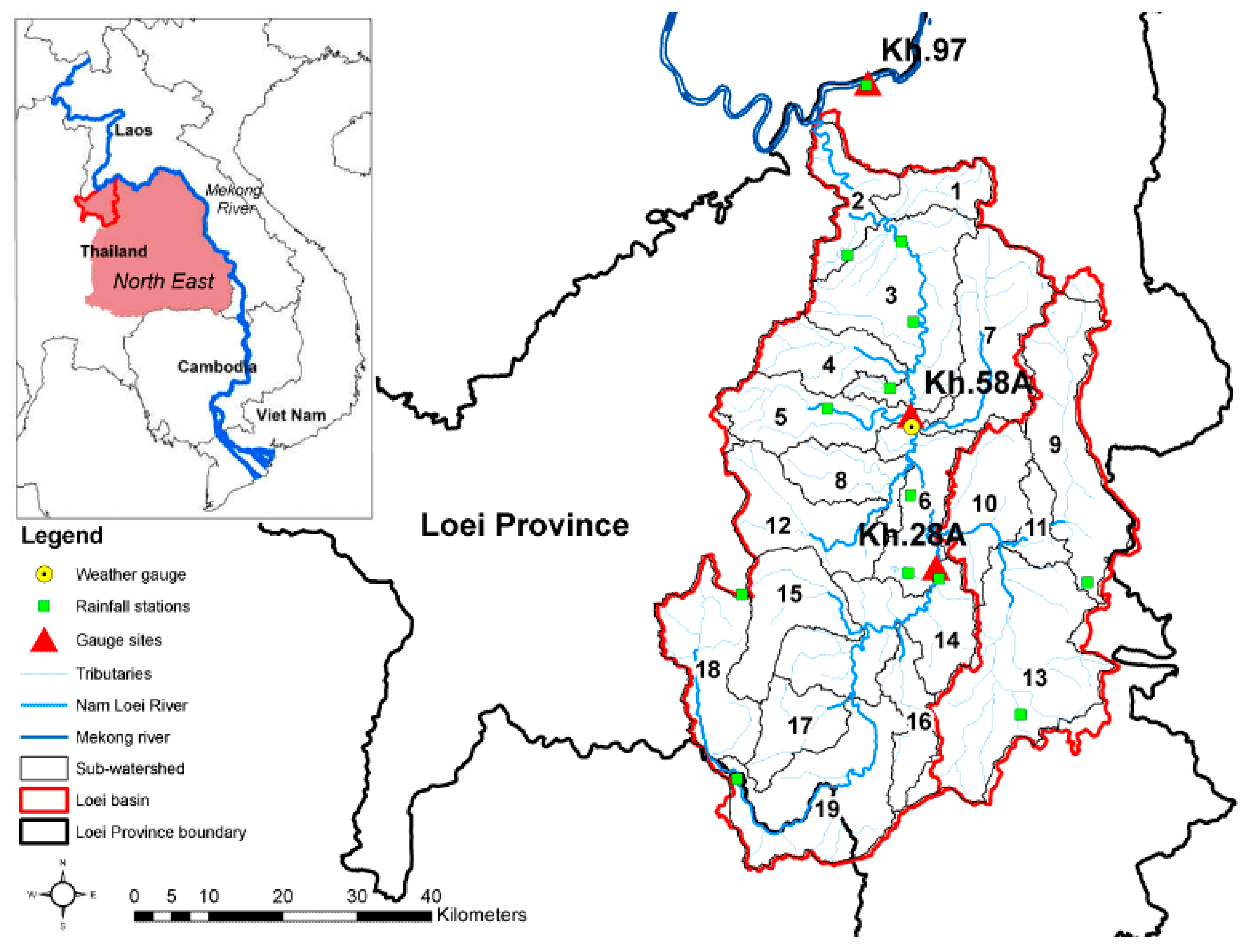
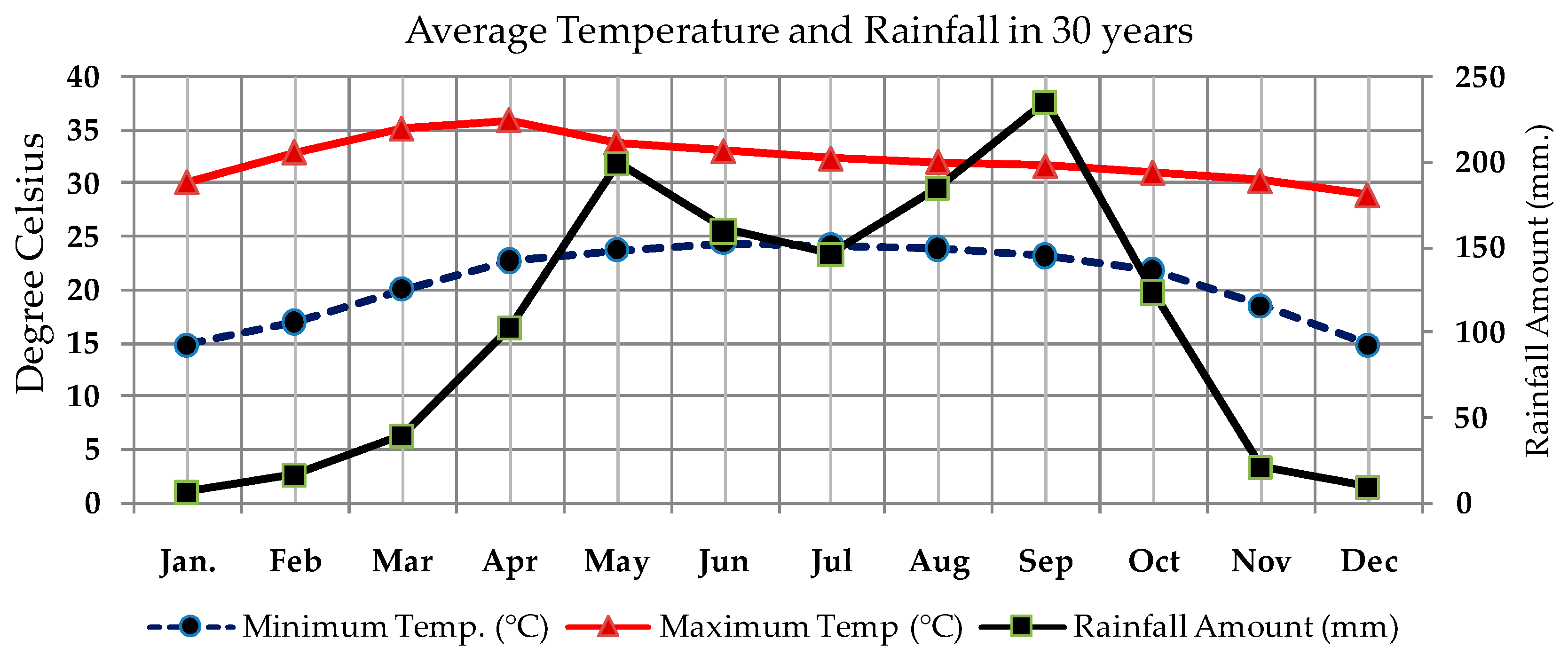
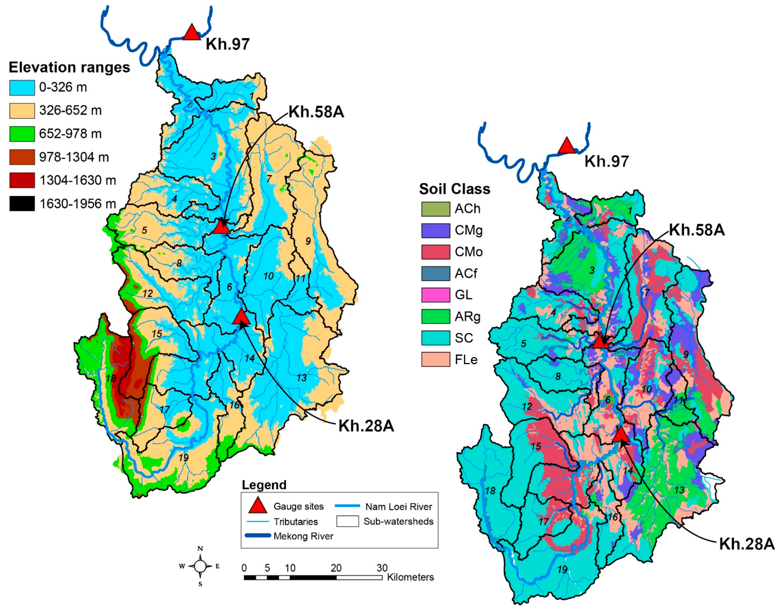
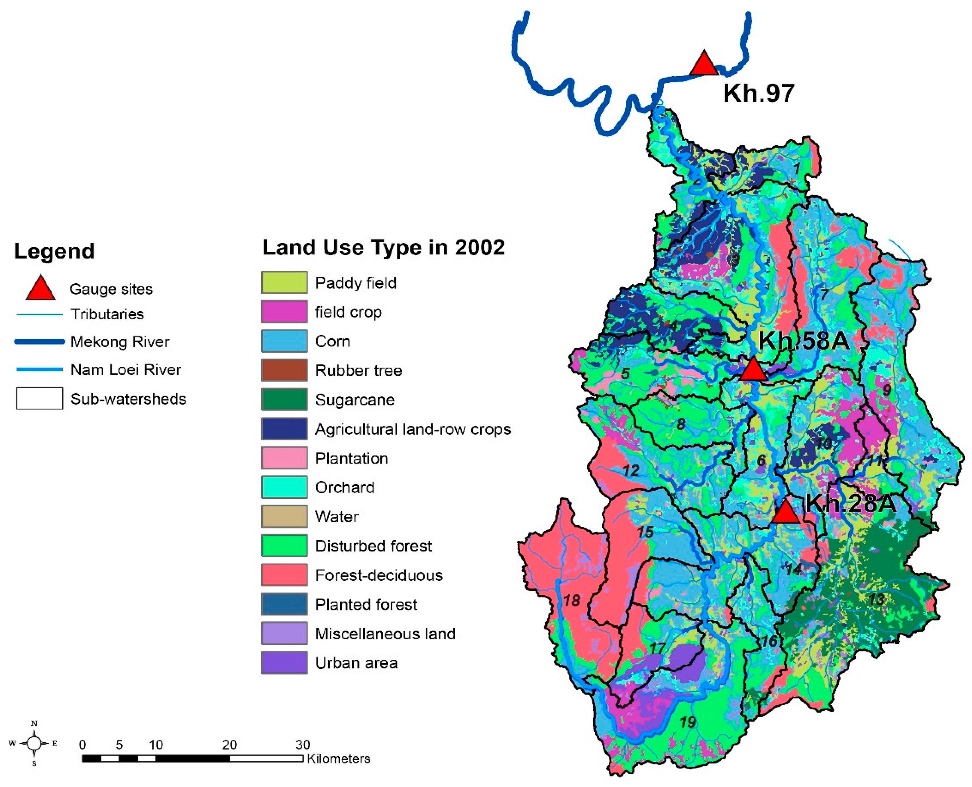
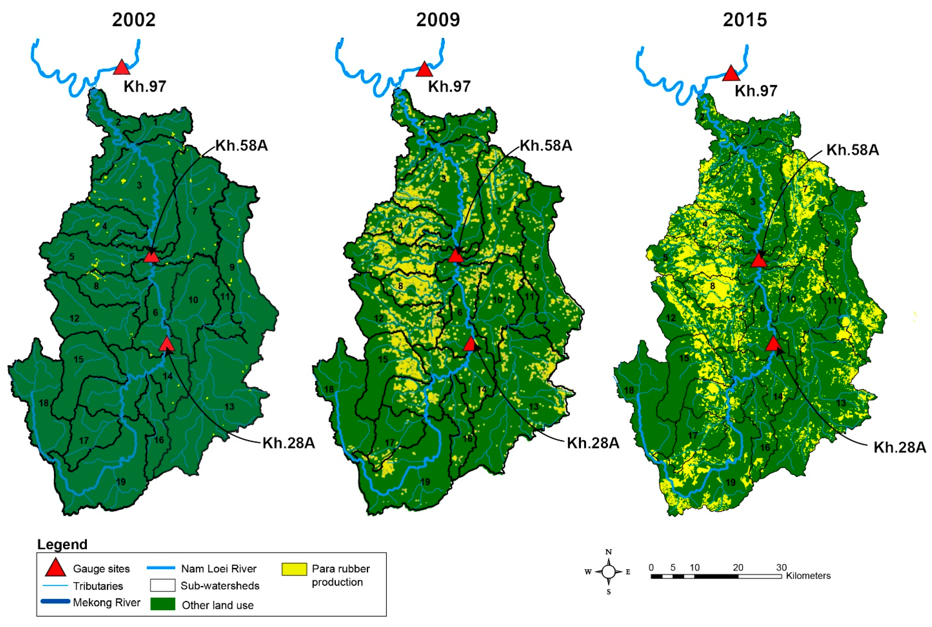
2.1. Description of Study Area

Loei Province covers 11,424 km2 in the upper northeastern region of Thailand (Figure 1) and is the fifth largest province in the region. The NLRB drains 3915 km2 from its combined upper basin and lower basin within Loei Province (Figure 1) and extends 231 km from the upper Phu Luang Range to its outlet. The Nam Puan is the major tributary of the upper basin, which is initially comprised of steep slopes but ultimately flows into a plain area where it joins the Nam Loei River within the Wang Sa Phung District. The main river of the lower basin is the Nam Loei River, which flows through the Muang District to the river plain within the Chiang Khan District to meet the Mekong River.
The average annual long-term rainfall and temperature is 1241 mm and 26.5 degree Celsius, respectively, for the NLRB [31]. The range of monthly average minimum temperatures, maximum temperatures, and precipitation over the 30-year period of 1981 to 2010 are shown in Figure 2 for climate station 48353, which is located in the study region [32]. However extended drought problems have resulted in streamflows of just 5% to 10% and 90% to 95% during the dry and rainy seasons, respectively, relative to annual average streamflow. Eight major groups comprise the spatial extent of soils in the NLRB, with the most dominant being the following three soil types: (1) the Slope complex (Sc) soil group which covers 44.3% of the basin, and represents a soil mixture in steep areas with >30% slopes that are generally characterized by forest, low permeability, and high risk of soil erosion; (2) the Wang hi (Wh) soil group, which covers 16.5% of the basin, represents soils derived from decay of various materials, and are characterized by fine-grain textures and high permeability; and (3) the Chiang Khan (Ch) soil group, which cover 14.4% of the basin, is derived from river sediments, and reflect sedimentary rock weathering and high permeability. Both the Wh and Ch soil types are prone to collapse or landslides in steep areas. The basin is further characterized by minimum, maximum and average elevations of 212 m, 1956 m, and 419 m, respectively. The land use of the basin, based on 2002 land use data [33], can be classified into 14 categories: corn (23.4%), disturbed forest (19.1%), forest–deciduous (12.5%), paddy field (12.3%), orchard (8.5%), sugarcane (5.9%), agricultural land-row crops (5.9%), field crop (4.8%), urban area (4.0%), miscellaneous land (1.7%), plantation (1.0%), water resources (0.4%), rubber tree (0.4%) and planted forest (0.2%). In 2002, the basin had a total Para rubber plantation area of just 762 ha. The plantation area then increased to 68,800 ha by 2009 and later to 100,000 ha by 2013, which met the expected goal established in a Para rubber production strategy for the NLRB [10]. However, Para rubber production has continued to increase since 2013, reaching 129,280 ha by 2015. Currently, the 2016 provincial policy points to an expansion of an additional 100,000 ha of Para rubber plantations in the next five years [34], which will result in almost double the land area currently dedicated to Para rubber production in the NLRB by 2020.

2.2. Evaluation of Evapotranspiation (ET) at the Basin Scale

Evapotranspiration (ET) is a collective term that includes all processes by which water at the earth’s surface is converted to water vapor. It includes evaporation from plant canopies, and sublimation and evaporation from soil. ET is usually the primary mechanism by which water is removed from a watershed. On average, ET equals about 62% of the precipitation that falls on landscapes across the globe except in Antarctica [35], where runoff exceeds ET. An accurate estimation of ET is critical in assessing the impact of climate and land use changes on water resources [36]. The water losses through ET are significant in the hydrologic cycle; such losses are usually determined by estimating the availability of water through soil moisture or groundwater, the energy and drying power of the air, and/or via land cover and vegetation characteristics [37]. A new method of determining ET for Para rubber trees has been developed in which the rubber tree ET is estimated by accounting for observed patterns of rubber root water uptake as affected by the plant’s phrenology [38]. Specifically, the method considers vegetation dynamics and corresponding water needs or evaporative demands. This contrasts with the traditional approach of estimating Para rubber ET, which neglects the increased water use during the dry season when both soil water content and canopy cover are minimal [38]. It is expected here that the SWAT basin-scale hydrologic model will more accurately capture seasonal water balance and ET dynamics that are more consistent with recent research, especially for larger scale rubber expansion situations that exceed smaller stand levels.

2.3. Description of SWAT Model

SWAT is a public domain model jointly developed by the U.S. Department of Agriculture Agricultural Research Service (USDA–ARS) and Texas AgriLife Research, a unit within the Texas A&M University System [15,16,17]. Watersheds are typically simulated in SWAT by delineating the respective watershed into subbasins and then further subdividing each subbasin into hydrologic response units (HRUs), which are non-spatial land units consisting of homogeneous topographic, soil type, land use, and management characteristics. Hydrologic cycling including precipitation inputs, surface runoff, infiltration into the soil profile, ET, lateral subsurface flow, and flow via other pathways is initially simulated at the HRU level. Nutrient cycling and transport, as well as sediment losses, are also simulated first at the HRU scale. The HRU-level hydrologic and pollutant outputs are then aggregated to the subbasin level and ultimately routed through the stream network to the watershed outlet.
SWAT first simulates atmospheric water demands to calculate the maximum, unstressed ET, commonly referred to as potential ET, before calculating the final actual ET. Three potential ET methods are included in SWAT that vary considerably in the amount of required inputs: (1) Penman–Monteith [39], which requires solar radiation, air temperature, relative humidity and wind speed; (2) Priestley–Taylor [40], which requires solar radiation, air temperature and relative humidity; and (3) Hargreaves [41], which requires air temperature only [11]. Multiple options are also provided in SWAT for simulating the partitioning of precipitation inputs between surface runoff and infiltration, as well as for some other processes simulated in the model. Complete theoretical and user input options are provided in the SWAT model documentation [36]. A revision of SWAT version 2009 (SWAT2009) was used in conjunction with the ArcGIS SWAT (ArcSWAT) interface for this study [42].

2.4. Application of SWAT

2.4.1. Data Input Needs and Sources

Topographic, soil, land use, climate, and management data are key inputs required for simulating a watershed in SWAT. In-stream monitoring data are also important in regards to testing SWAT output. Topographic, soil, and land use are usually input into SWAT in the form of digital spatial layers that are overlaid within a Geographic Information System (GIS). All of these major data were prepared in input format files for the SWAT simulations including spatial topographic, soil and land use data (Table 1, Figure 3 and Figure 4) obtained from various sources as described below.
Spatial topographic data required for the SWAT application were obtained in the form of a digital elevation map (DEM) [43]. These DEM data are characterized by a 30 m × 30 m (1:50,000 scale) resolution. The baseline land use data for year 2002 [44] and the spatial soil map were provided by the Land Development Department [45]. The LDD soil data consist of the previously mentioned 8 major groups. All soil properties required for SWAT were surveyed from by the LDD in 2012 [46]. Daily climate data were used, including precipitation, temperature, solar radiation, wind speed, and humidity data. These data were collected from rainfall gauges within the NLRB during the period from 1985 to 2015 [32]. The daily precipitation data were obtained at 14 gauging stations (Figure 1), while the daily temperature, solar radiation, wind speed and humidity data were collected from a single major weather station (Figure 1) of the Thai Meteorological Department (TMD). Two hydrologic runoff stations located in the basin (gauges Kh.28A and Kh.58A in Figure 1) that are maintained by the Royal Irrigation Department (RID) and have complete monthly runoff data were selected for model calibration and validation [47].

2.4.2. Model Set Up

The NLRB was delineated into 19 subbasins and 389 hydrologic response units (HRUs) for the SWAT simulations using the ArcSWAT Interface [42]. The delineation was performed as a function of the DEM-based surface topography, which resulted in the configuration of the 19 sub basins used in the SWAT simulations. The land use data were processed and reclassified to match the land use codes used in SWAT, resulting in the previously described 14 land use categories. The eight major soil types were also converted and reclassified to match the SWAT model soil formatting requirements. These land use and soil data were then overlaid with the DEM data within ArcSWAT to create the HRUs. The required weather data were incorporated or the simulations. The initial curve number values were assigned based on the land use type and soil hydrologic group for the average antecedent moisture condition of the runoff curve number method. The PET was computed by using the Penman–Monteith method. The overall model simulation scenario period covered a 25-year duration from 1985 to 2009 using a daily time step, with a shorter time period used for model calibration and validation as described below.

2.4.3. Sensitivity Analysis and SWAT Calibration and Validation

A sensitivity analysis is a useful procedure to determine which flow-related parameters are the most influential in impacting total streamflow for SWAT applications, following guidance reported for previous studies [16,48,49,50,51]. Performing a sensitivity analysis further supports the calibration of SWAT and provides insight for the application of the model to other similar watersheds. In this study, the SWAT CUP software package [52] was used to perform an automatic sensitivity analysis of the impact of 19 different SWAT parameters on daily streamflow flow for the NLRB as described in the Results and Discussion section.
Following the sensitivity analysis, calibration and validation of SWAT was performed which is required to reduce uncertainty and increase confidence in its predictive abilities for the NRLB [16,49,50]. The calibration process included both multisite and multivariable aspects as discussed in previous SWAT studies [16,50]. The calibration procedure consisted of 3 stages: (1) replicating the long-term water balance over the calibration period; (2) accurately tracking the observed hydrograph shapes; and (3) obtaining an accurate comparison between observed and simulated flow duration curves. Calibration and validation of SWAT was performed by comparing the simulated monthly aggregated stream flows versus corresponding measured monthly stream flows at two hydrological gauge stations on the main stem of the Nam Loei River (Figure 1): Wang SaPhung (Kh.28A) in subbasin 14 and Ban FakLoei (Kh.58A) in subbasin 6. Calibration was performed for 1994 to 2004 while validation was conducted from 2005 to 2009. The parameters derived for the gauged catchments were then transferred to the ungauged catchments, based on proximity and similarities in land use and soil types which result in similar hydrological responses.
The accuracy of the model output variance was assessed using the Root Mean Squared Error (RMSE) and Nash–Sutcliffe Efficiency (NSE) statistics [53,54], which are expressed as follows in Equations (1) and (2):
RMSE = i = 1 n ( Q i o b s Q o b s ¯ ) ( Q i s i m Q s i m ¯ ) i = 1 n ( Q i o b s Q o b s ¯ ) 2 i = 1 n ( Q i s i m Q s i m ¯ ) 2
NSE = 1 [ i = 1 n ( Q i O b s Q i S i m ) 2 i = 1 n ( Q i O b s Q m e a n ) 2 ]
where Qobs are the observed values and Qsim are the simulated values at time/place i.
Values of RMSE can range from 0 to ∞ where a value of 0 indicates a perfect fit between the simulated data and counterpart measured data [53]. The RMSE provides a measure of the difference between the measured and simulated values or residual variance [55]. However, statistical results generated with the RMSE can result in significant model bias during model calibration, even when the error variances are small [56]. Thus it is desirable to use additional statistical evaluation when using the RMSE such as the NSE.
The NSE estimates the magnitude of the simulated variance relative to the measured variance and how accurately a plot of the modeled versus measured data fit a 1:1 line. The NSE can vary from −∞ to 1, where 1 is a perfect fit and a negative value indicates that the average value of the measured data would provide a better prediction than the simulated data. Statistical criteria for judging the success of hydrological modeling results has been suggested [55,57] including an NSE value of at least 0.5 to achieve a satisfactory level for comparisons of aggregate monthly simulation output versus corresponding measured stream flow data. Following successful calibration and validation, the calibrated SWAT model was used to evaluate the Para rubber land use scenario (describe below) including evaluations of ET and water yield.

2.5. Development of Para Rubber Land Use Scenarios

Several factors need to be considered in developing the Para rubber land use scenarios for the NLRB. First, it is important to consider the optimal climatic, soil, slope, and other conditions that Para rubber should be grown under for the study region, especially in the context of typical current practices in which rubber plantations are being established on very high, vulnerable slopes. Second, crop parameters needed to be developed for Para rubber for this analysis. Third, 2002 baseline, 2009 scenario and 2015 scenario landuse layers had to be constructed in order to simulate the impact of expanded Para rubber production in the NLRB during the period of rapid production expansion. These aspects of the Para rubber scenario development are described below.

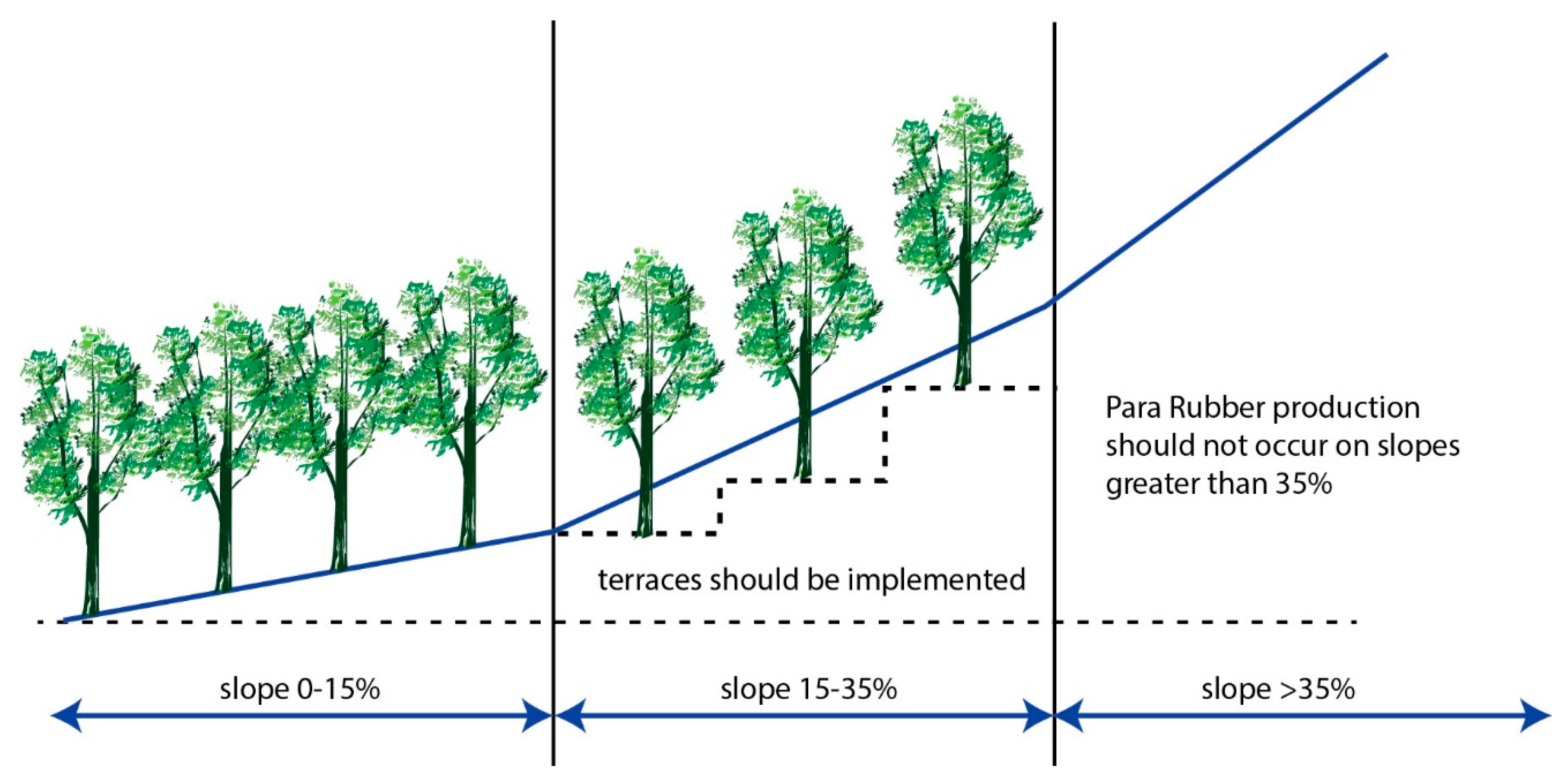
2.6. Optimal Environmental Conditions for Para Rubber Production

The rubber tree is native to the evergreen tropical rainforests which usually occur within 5° latitude of the equator. The climate of this region is characterized by heavy rainfall and no distinct dry season [5]. The optimal climatic conditions for Para rubber include rainfall of 1250 mm or more, evenly distributed throughout the year with no severe dry season and with 120–150 annual rainy days, and a temperature range of about 26–30 °C [34]. In addition, the ideal elevation range for Para rubber growth is from sea level up to 600 m above mean sea level; the growth rate will decline at higher altitudes. Para rubber can grow on many soils, with the best options being well drained clayey and deep clay soils, but it can withstand physical conditions ranging from stiff clays with poor drainage to well drained sandy loams [5]. The most suitable soil conditions for Para rubber production are: (1) planted at a depth which does not exceed 1 m in depth to allow for adequate future root penetration and growth; (2) soil textures that range between loamy sand to clay loam with good drainage; (3) no gravel or stone in the subsoil layer; and (4) the soil pH should range between 4.5 and 5.5 [34].
The ideal slope range for growing Para rubber trees is between 5% and 15%. Three categories can be classified for this ideal range for the Loei River basin region: (1) low land areas with slopes from 0% to 5%; (2) slopes ranging from 5% to 10% located in the plain areas; and (3) mild slopes that typically range from 10% to 15%. About 30% (117,433 ha) of the total area within the basin region meets these ideal slope characteristics [58]. However, the majority of the current Para rubber production in the study region is currently occurring on much steeper slopes exceeding 15%, and is concentrated especially in an extreme slope range of 30% to 35%. Therefore, Para rubber production on slopes greater than 15% should be managed with terraces as shown in the photos and schematic in Figure 5. It was outside the scope of the present research to account for such terrace systems as part of the SWAT simulations reported in this study.

2.7. Para Rubber Crop Parameters

Crop growth in the SWAT model was set up for this study primarily using a heat unit schedule approach. However, rice and other “field crops” were simulated for two growing seasons during each year and thus both were simulated using specific planting and harvesting dates rather than heat unit scheduling. Double cropping of wet season rice and dry season rice were accounted for in the simulation; the second dry season crop is mostly grown in selected areas of Thailand that have sufficient irrigation water available. The planting schedules of wet season rice, dry season rice and field crops were simulated based on typical planting dates for each crop type in the region. The remaining operations were controlled by the fraction of heat units for each crop using the heat unit scheduling approach [36].
Para rubber is a perennial tree crop which grows year round; thus, annual planting and harvest and operations were not simulated for Para rubber. Para rubber crop parameters were not available in the ArcSWAT database for SWAT2009; thus, parameters had to be determined from measured data, inferred from existing parameters for other tree species in the ArcSWAT database, or determined from other sources. Values for 15 key Para rubber Tree (RUBR) crop parameters, and two other vegetation-influenced input parameters, which were used for the NLRB SWAT analysis, are listed in Table 2. The value selected for the maximum canopy height (CHTMX) were based on previously reported measurements [5] while the maximum rooting depth (RDMX) value is based on other measurements conducted by Thai scientists [58]. The other crop parameters in Table 2 were derived mainly from existing tree crop parameters in the ArcSWAT database. The choice of curve number (CN2) value for Para rubber trees reflects a woodland condition consisting of a thin stand, poor cover, no mulch, and a soil type consistent with hydrologic soil group B drainage conditions [59]. The Manning’s n value for overland flow (OV_N) represents high runoff for timberland conditions [60]. Minimum, maximum and average values are listed for each crop parameter in Table 2. These parameter ranges allow the user the flexibility to decrease or increase the crop parameter default values, typically by approximately 10%.
Finally, the daily rubber tree water requirement rate was calculated by using the Bowen Ratio method based on data collected for 10-year old rubber trees at an experimental site in Chachoengsao Province. Temperature and humidity sensors were installed within and above the rubber tree canopy at the site. Solar radiation and wind velocity sensors were also installed above the rubber tree canopy. Soil temperature and soil moisture sensors were installed at 0 m and 0.10 m depths. A S-shape regression had been proposed to describe the relation between crop coefficients (Kc) and the Julian date. Therefore, the S-shape regression can be applied to evaluate the water requirement of rubber trees at different locations beyond the experimental site [61].

2.8. Land Use Change Scenarios

Table 3 shows the specific land use distributions for the 2002, 2009 and 2015 land use scenarios, and the percentage difference for each land use category for two time periods: (1) between 2002 and 2009; and (2) between 2009 and 2015. The major changes in land use between 2002 and 2009 included a nearly 11.5% increase in Para rubber production, a decline in corn production of 10%, a decrease in disturbed forest land of over 9.7%, and increases in evergreen and deciduous forest of 7.35% and 2.1%, respectively. The largest shift in land use between 2009 and 2015 was an increase in Para rubber production of 9.69%, which was primarily responsible for respective decreases of −3.57%, −2.99%, −1.93%, −1.84% and −1.77% of corn, disturbed forest land, sugarcane, paddy fields and orchards.
The distribution of Para rubber production is also shown in the 2002 baseline land use map, versus the 2009 and 2015 land use scenario maps, in Figure 6. These distributions of Para rubber production areas further underscore the dramatic expansion of Para rubber tree plantations that occurred during the 14-year period of 2002 to 2015 in the NLRB. The effects of the increase in Para rubber production between the 2002 baseline and the two scenario years of 2009 and 2015 were accounted for in three separate scenario simulations performed in SWAT. The baseline scenario was first executed using the 2002 land use distribution (Table 3) for a 25-year period (1985 to 2009). The 2009 and 2015 land use scenarios were then performed for the same 25-year period to provide a consistent basis of comparison versus the baseline scenario.

3. Results

3.1. Sensitivity Analysis

The top five most sensitive parameters as ranked in Table 4 were: (1) ALPHA_BF, base flow alpha factor (days); (2) ESCO, soil evaporation compensation factor; (3) GQWMN, threshold depth of water in the shallow aquifer required for return flow to occur (mm); (4) CN2, initial SCS runoff curve number for moisture condition II; and (5) CH_K2, effective hydraulic conductivity in main channel alluvium (mm·h−1). The most influential parameters found in the sensitivity analysis are consistent with previously published summaries of the most widely used parameters in SWAT calibration [16,50]. The results also underscore the importance of accurate spatial and temporal precipitation inputs [16,50]. The choice of ALPHA_BF, CN2, ESCO and other parameters also varied (Table 4) between the two subbasins that drain to gauges Kh.28A and Kh.58A, respectively.

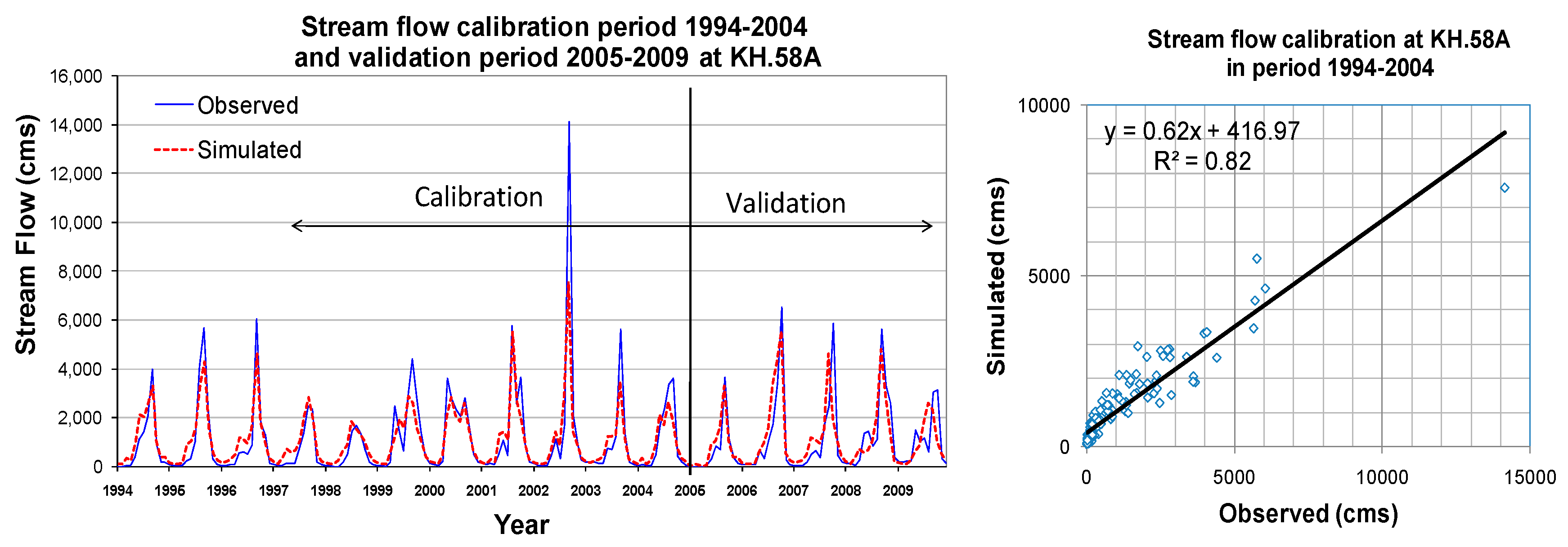
3.2. Model Calibration and Validation

The statistical results of comparing the simulated SWAT calibration and validation aggregated monthly streamflows versus corresponding measured streamflows are listed in Table 5 for both gauge sites (Figure 1). The graphical comparisons between the simulated and measured monthly streamflows for the calibration and validation period are shown in Figure 7 for gauge site Kh.58A. The four NSE values computed for the two gauges during the calibration and validation period all exceeded 0.5, indicating that SWAT produced satisfactory streamflow estimates per previously suggested criteria [55,57]. The RMSE statistics were also all below 1.0 which further confirm that the SWAT streamflow estimates satisfactorily replicated the measured streamflows.
The graphical comparisons between the simulated and measured aggregated monthly streamflows for the calibration and validation period at gauge site Kh.58A (Figure 7) show that SWAT accurately replicated most of the measured streamflow trends during the 11-year calibration period. However, several peak monthly streamflows were under predicted, especially in the last three years of the calibration period, which mirrors a tendency towards under prediction reported in a number of existing SWAT studies (e.g., [15]) and points to the need for further improvement of the SWAT hydrological algorithms, especially for Southeast Asia conditions. Similar graphical results occurred for the other three gauge site/time period combinations and thus are not reported here.

3.3. Overall Water Balance Results for the Land Use Scenarios

Table 6 shows the overall long-term average annual water balance results for the entire NLRB predicted by SWAT for the 25-year 2002, 2009 and 2015 land use scenario simulations. The results of the scenarios reflect the increases in Para rubber production and other shifts in land use that occurred during the 2002 to 2009 and 2002 to 2015 time periods. Transmission losses were essentially negligible for all three land use scenarios, and the estimated combined lateral subsurface flow and groundwater flow were very similar between the three scenario simulations. However, the predicted ET increased by nearly 17 mm, and the predicted surface runoff and water yield decreased by similar amounts for the 2009 land use scenario as compared to the 2002 land use scenario. Similar, greater decreases in reduced surface runoff and water yield, relative to the 2009 land use scenario, were estimated for the 2015 land use scenario. However, the simulated ET decreased by almost 12 mm between the 2015 and 2009 land use scenarios. These results underscore the impacts of both the increased Para rubber production and shifting overall land use mixes in the NLRB between 2002 and 2015 (Table 3).

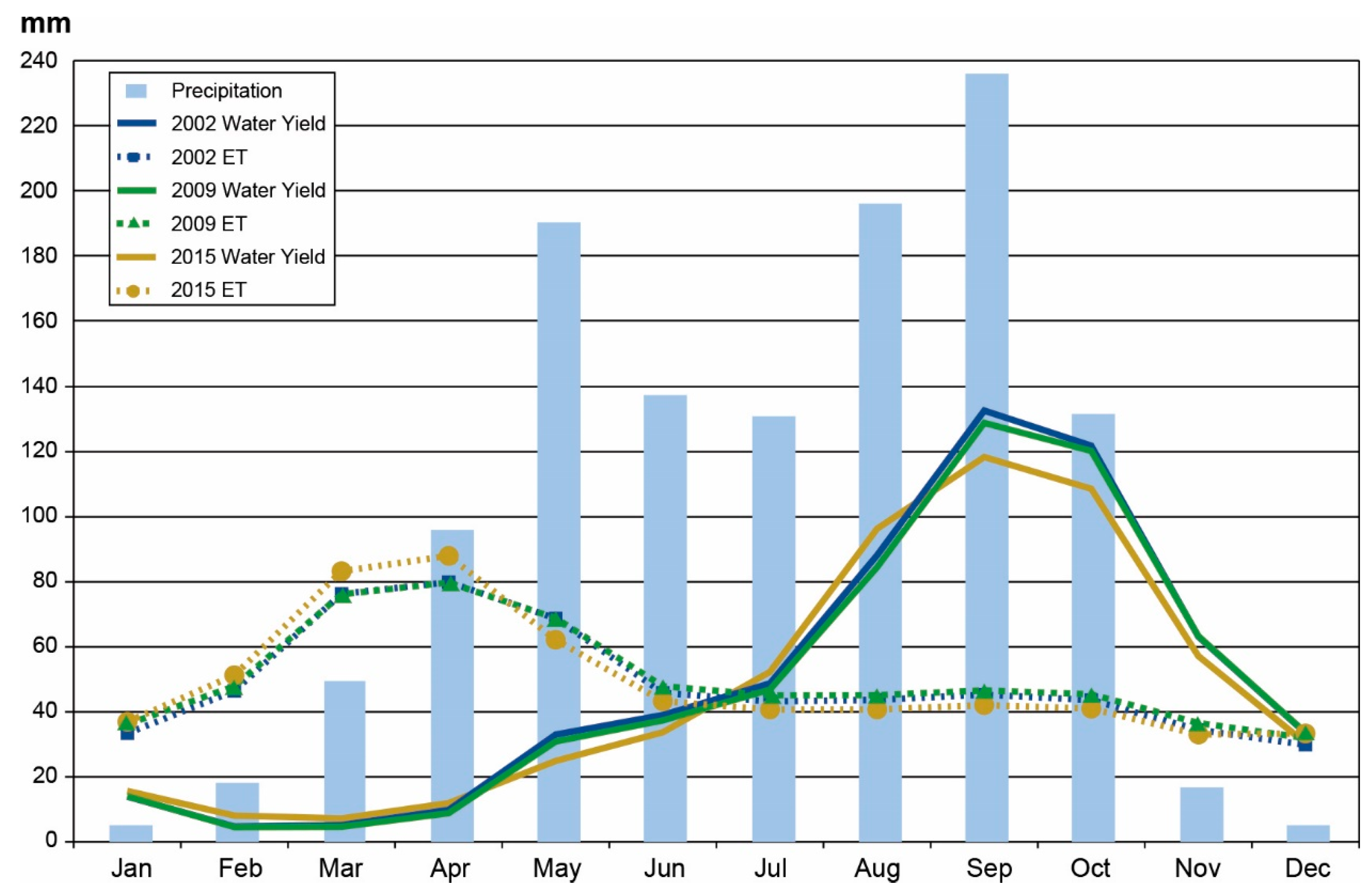
3.4. Seasonal ET and Water Yield Responses

The 25-year average monthly precipitation, ET levels and water yields simulated for the 2002, 2009 and 2015 NLRB land use scenarios during the 25-year simulation period (1985 to 2009) are shown in Figure 8. The initial increase in Para rubber plantations and other land use changes that had occurred by 2009 (Table 3) resulted in predicted increases in ET in almost every month of the year, relative to the baseline year of 2002 (Figure 8), except for March and April. The annual average ET increased about 3% (Table 6), with the highest percentage increases occurring during the dry season months of November to January and the lowest percentage increases occurring during the wet season months of May, September and October. The estimated water yield responses between the baseline and 2009 Para rubber expansion scenario resulted in the opposite trend, with water yields decreasing in most months, although slight increases occurred during the months of November, December and January. The predicted percentage water yield changes ranged from +0.6% in January to over −10% in March and April. The percentage declines in water yield predicted for the wet season were more constant as compared to the dry season water yield impacts, ranging from −1% in October to −7% in October.
The continued expansion of Para rubber production and other land use changes between 2009 and 2015 (Table 3) resulted in stronger shifts in the predicted monthly ET levels and in the annual hydrograph (Figure 8), with an earlier onset of the flood season and a decreased overall peak discharge in September. The estimated ET for the 2015 land use scenario was higher during the dry season as compared to 2002 and 2009 (Figure 8), except for November, but the opposite trend occurred during the wet season, resulting in an overall decline of about 2% from 2009 to 2015 (Table 6). The overall average dry period water yield was predicted to be about 13% higher for the 2015 land use scenario as compared to the baseline during November to April. However, lower water yields were predicted during most of the wet period except for the months of July and August (Figure 8). In total, the average annual simulated water yield decreased almost 7% from the baseline to 2015 (Table 6).
Table 7 provides comparisons of: (1) the long-term (25-year simulation period) average cumulative amounts of ET (mm) and water yield (mm) that occurred during the wet season, dry season, and annually; (2) the percentages of the cumulative amounts that occurred during the wet season and dry season; and (3) the percentage changes in annual average ET and WYLD that occurred due to the land use changes between 2002 and 2009, and 2009 and 2015. These results show that nearly 80% of the water yield occurred during the wet season during both the 2002 baseline and the 2009 and 2015 Para rubber expansion land use scenarios (Table 7), as compared to the dry season. However, a more even distribution of ET occurred between the wet and the dry seasons, with slightly higher levels occurring during the dry season. Slight shifts in the overall amounts that occurred between the two seasons were generally predicted for the 2009 and 2015 conditions relative to the 2002 baseline; the 2015 land use scenario ET estimates resulted in the largest relative shift that was predicted between the two seasons (Table 7).
Various seasonal shifts were predicted to occur between 2002 baseline and the 2009 landuse scenarios, and between the 2009 and 2015 land use scenarios (Table 7). Relatively minor shifts were estimated between 2002 and 2009, with ET increasing by roughly 3% in both seasons versus 1% and 3% declines in water yield for the dry season and wet season, respectively. ET was predicted to decrease almost 10% during the wet season but increase nearly 6% during the dry season, between 2009 and 2015. In contrast, water yield was predicted to decrease during the wet season by about 3% and increase by 1% during the dry season, between the two landuse scenarios. The estimated average annual percentage change in ET from 2002 to 2009 was a decline of roughly 3% as compared to an increase in water yield of close to 3% for the same time period (Table 7). In contrast, the predicted average annual percentage change in both ET and water yield from 2009 to 2015 was a decline of roughly 2% (Table 7).

4. Discussion

As noted previously, substantial increases in rubber tree production are expected to occur in Southeast Asia by 2050. Preliminary research suggests that this massive land use change could exacerbate environmental problems in the region including increased soil erosion and sediment transport to surface water, degraded soil quality, decreased stream flow, risk of landslides and probable decreased soil carbon levels [1,2,62]. The majority of the area where rapid and widespread land conversion to monoculture rubber plantation has occurred in continental SE Asia is also vulnerable to extreme climatic events including typhoons, frost or drought, which can greatly reduce or even destroy rubber production and further exacerbate environmental problems [3]. Furthermore, these environmental problems may be magnified even more per projected future climate change in the region [3]. Intensified Para rubber production has also negatively impacted biodiversity in production areas located in Thailand and other subregions in Southeast Asia [63].
The results of this study show that the expansion of rubber cultivation is resulting in a decreased volume of water in the rainy season in the NLRB in northeast Thailand. In addition, during the dry season the water content decreases, resulting in water shortages. The expansion of rubber production in inappropriate areas with slopes over 35% [51] is more likely to result in increased flash floods and landslides due to the intensive monoculture practices. This is especially true for the Nam Manh, Nam Phu and Nam Paow subbasins, where 3000 ha of Para rubber plantations have been introduced on landscapes with extremely high slopes. In addition, an additional 10,300 ha of Para rubber production exists in more moderate slope areas (15% to 35% slopes) that are distributed across the upper, middle and lower subregions of the NLRB. The Rubber Research Institute of Thailand has recommended that terrace systems should be used for rubber production on slopes >15% [34] but this recommendation is not being consistently followed. These specific problems occurring in Thailand, coupled with the previously described environmental problems that are increasing Southeast Asia, underscore the urgent need to develop measurement approaches, databases and modeling tools that can be used to investigate Para rubber production problems throughout the region.
The amount of water that is required to initiate and sustain Para rubber plant growth depends on many factors such as the type of plant species, the age of the plant and weather conditions such as wind speed, temperature and humidity [61]. There are many ways to determine crop water use both directly and indirectly. The measure by instrumentation is more accurate, but cannot be conducted across large plantations. The application of mathematical models is a popular method and are widely used in the study and evaluation of water use and water requirements of crops, which saves time and cost. However, the use of mathematical models can require extensive input data depending on the type and format of the model. There are parameters that must be calibrated and verified to ensure the calculated results are close to the measured values. Furthermore, databases with appropriate parameter values may not be available for some models. Thus, those databases must be brought up-to-date to better meet the needs of end users.
The case study reported here that describes the expansion of Para rubber plantations in the NLRB using SWAT is an example of an application that requires the development of important plant input parameters. However, there is a need to further develop SWAT Para rubber input parameters that better account for rubber species and age, rubber stems and leaves of rubber trees. In addition, there is a need to improve the SWAT growth functions to be able to better account for the effects of rubber tree growth phenomena related to the rooting structure that depletes deeper soil layers and results in higher ET impacts, relative to traditional vegetation [36,64]. Finally, an overall expanded Para rubber production and knowledge database is needed for Thailand and Southeast Asia in general.

5. Conclusions

The Soil and Water Assessment Tool (SWAT) model was applied to assess the impact of Para rubber expansion in the Nam Loei River Basin in this study The application has designated the land use in the year 2002 as the baseline versus historical Para rubber tree expansions in 2009 and 2015 as the land use change scenarios. The stream flow estimated by SWAT showed annual average stream flow of about 1580 MCM. The average stream flow occurring during the rainy season (June–November) was about 1264 MCM (80% of the average annual stream flow) and in the dry season about 316 MCM (20% of the average annual stream flow). The simulation was done using scenarios to assess the water balance in the hydrological process. The results of the simulations showed that the increased production of Para rubber, which replaced the original local field crop and disturbed forest land, resulted in an increase of ET of about 3% from 2002 to 2009. However, additional increased Para rubber production in combination with other land use shifts during 2009 to 2015 resulted in a predicted ET decrease of 2%. The major factors that influenced this result were the rubber canopy and precipitation. Moreover, runoff results reduced water balance in the basin by an annual average of about 3%, especially during the dry season. However, the effect of ET on water resources has increased complexity and uncertainty; the consideration of many parameters of Para rubber and a reflection on the past will help our understanding of the dynamic changes. The results of this study will help provide guidance for decision-making about land use allocation or zoning for suitable Para rubber area. In addition, this study will aid in the management and planning of water resources for the NLRB and other river basins located in northeastern Thailand.

Acknowledgments

This study was carried out as part of the required research to fulfill Ph.D. thesis requirements for the Graduate School of Kasetsart University. The authors would like to express their sincere thanks to the Thailand Research Fund (TRF) through the Royal Golden Jubilee Ph.D. Program and Kasetsart University Research and Development Institute (KU–RDI) for their financial support. We would also like to thank the Department of Water Resources, Land Development Department and other agencies for supplied the data for the study.

Author Contributions

Winai Wangpimool performed the model input data collection and analysis, modeling work and primary analysis of the results. Kobkiat Pongput provided guidance regarding the methodology, literature review and the results and conclusions of the study. Nipon Tangtham provided guidance regarding the development of Para rubber plant parameters and trends in Para rubber production. Saowanee Prachansri provided consultation regarding the land use and soil data including specific input parameters. Philp W. Gassman provided guidance regarding the methods used in the study, contributed in-depth analysis of the simulation results and provided editing and writing support.

Conflicts of Interest

The authors declare no conflict of interest.

References

  1. Ziegler, A.D.; Fox, J.M.; Xu, J. The Rubber Juggernaut. Science 2009, 324, 1024–1025. [Google Scholar] [CrossRef] [PubMed]
  2. Fox, J.; Castella, J.C. Expansion of rubber (Heveabrasiliensis) in mainland southeast Asia: What are the prospects forsmallholders? J. Peasant Stud. 2013, 40, 155–170. [Google Scholar] [CrossRef]
  3. Ahrends, A.; Hollingsworth, P.M.; Ziegler, A.D.; Fox, J.M.; Chen, H.; Su, Y.; Xu, J. Current trends of rubber plantation expansion may threaten biodiversity and livelihoods. Glob. Environ. Chang. 2015, 34, 48–58. [Google Scholar] [CrossRef]
  4. Mongkolsawat, C.; Putklang, W. An Approach for Estimating Area of Rubber Plantation: Integrating Satellite and Physical Data over the Northeast Thailand. 2010. Available online: http://a-a-r-s.org/aars/proceeding/ACRS2010/Papers/Oral%20Presentation/TS36-1.pdf (accessed on 22 August 2016).
  5. Rantala, L. Rubber Plantation Performance in the Northeast and East of Thailand in Relation to Environmental Conditions. Master’s Thesis, University of Helsinki, Helsinki, Finland, 2006. [Google Scholar]
  6. Suwanwerakamtorn, R.; Putklang, W.; Khamdaeng, P.; Wannaros, P. An Application of THEOS Data to Rubber Plantation Areas in Mukdahan Province, Northeast Thailand. 2012. Available online: http://gecnet.kku.ac.th/research/i_proceed/2555/2_ip2012.pdf (accessed on 4 June 2013).
  7. Office of Agricultural Economics. Agricultural Statistics of Thailand 2009; Center for Agricultural Information, Office of Agricultural Economics: Bangkok, Thailand, 2009; pp. 78–81, No. 401.
  8. Office of Agricultural Economics. Agricultural Statistics of Thailand 2010; Center for Agricultural Information, Office of Agricultural Economics: Bangkok, Thailand, 2010; pp. 78–81, No. 416.
  9. Office of Economic and Social Development of Northeastern. Para Rubber Situation and Adaptation of Farmers in the Northeastern; The Office of the National Economic and Social Development: Khon Kean, Thailand, 2015; p. 47.
  10. Prakhonsri, P. The Fires in the Northeast and Management. Technical Conference of Management of Natural Disasters in the Northeast and the Self-Reliance of Local Sustainable. 2011, pp. 42–47. Available online: http://www.tndl.org/kku/pdf/fire-prasit.pdf (accessed on 22 August 2016).
  11. Chakarn, S.; Soontorn, K.; Niwat, A.; Jitti, P. Growths and carbon stocks of Para rubber plantations on Phonpisai soil series in northeastern Thailand. Rubber Thai J. 2012, 1, 1–18. [Google Scholar]
  12. Bowen, G.D.; Nambiar, E.K.S. Nutrition of Plantation Forests; Academic Press: London, UK, 1989; p. 505. [Google Scholar]
  13. Arnold, J.G.; Srinivasan, R.; Muttiah, R.S.; Williams, J.R. Large area hydrologic modeling and assessment part I: Model development. J. Am. Water Resour. Assoc. 1998, 34, 73–89. [Google Scholar] [CrossRef]
  14. Gassman, P.W.; Reyes, M.; Green, C.H.; Arnold, J.G. The soil and water assessment tool: Historical development, applications and future directions. Trans. ASABE 2007, 50, 1211–1250. [Google Scholar] [CrossRef]
  15. Williams, J.R.; Arnold, J.G.; Kiniry, J.R.; Gassman, P.W.; Green, C.H. History of model development at Temple, Texas. Hydrol. Sci. J. 2008, 53, 948–960. [Google Scholar] [CrossRef]
  16. Arnold, J.G.; Moriasi, D.N.; Gassman, P.W.; Abbaspour, K.C.; White, M.J.; Srinivasan, R.; Santhi, C.; Harmel, R.D.; van Griensven, A.; van Liew, M.W.; et al. SWAT: Model use, calibration and validation. Trans. ASABE 2012, 55, 1491–1508. [Google Scholar] [CrossRef]
  17. Gassman, P.W.; Sadeghi, A.M.; Srinivasan, R. Applications of the SWAT model special section: Overview and Insights. J. Environ. Qual. 2014, 43, 1–8. [Google Scholar] [CrossRef] [PubMed]
  18. Gassman, P.W.; Wang, Y. IJABE SWAT Special Issue: Innovative modeling solutions for water resource problems. Int. J. Agric. Biol. Eng. 2015, 8, 1–8. [Google Scholar]
  19. Bressiani, D.A.; Gassman, P.W.; Fernandes, J.G.; Garbossa, L.H.P.; Srinivasan, R.; Bonumá, N.B.; Mendiondo, E.M. A review of soil and water assessment tool (SWAT) applications in Brazil: Challenges and prospects. Int. J. Agric. Biol. Eng. 2015, 8, 9–35. [Google Scholar]
  20. Krysanova, V.; White, M. Advances in water resources assessment with SWAT: An overview. Hydrol. Sci. J. 2015, 60, 771–783. [Google Scholar] [CrossRef]
  21. Babel, M.S.; Shrestha, B.; Perret, S.R. Hydrological impact of biofuel production: A case study of the KhlongPhlo Watershed in Thailand. Agric. Water Manag. 2011, 101, 8–26. [Google Scholar] [CrossRef]
  22. Glavan, M.; Pintar, M.; Volk, M. Land use change in a 200-year period and its effect on blue and green water flow in two Slovenian Mediterranean catchments: Lessons for the future. Hydrol. Process. 2012, 27, 3964–3980. [Google Scholar] [CrossRef]
  23. Jha, M.; Schilling, K.E.; Gassman, P.W.; Wolter, C.F. Targeting land-use change for nitrate-nitrogen load reductions in an agricultural watershed. J. Soil Water Conserv. 2010, 65, 342–352. [Google Scholar] [CrossRef]
  24. Kim, Y.; Band, L.E.; Song, C. The influence of forest regrowth on the stream discharge in the North Carolina Piedmont watersheds. J. Am. Water Resour. Assoc. 2013. [Google Scholar] [CrossRef]
  25. Liu, W.; Cai, T.; Fu, G.; Zhang, A.; Liu, C.; Yu, H. The streamflow trend in Tangwang river basin in northeast China and its difference response to climate and land use change in sub-basins. Environ. Earth Sci. 2012, 69, 1–12. [Google Scholar] [CrossRef]
  26. Ma, X.; Xu, J.; van Noordwijk, M. Sensitivity of streamflow from a Himalayan catchment to plausible changes in land cover and climate. Hydrol. Process. 2010, 24, 1379–1390. [Google Scholar] [CrossRef]
  27. Memarian, H.; Tajbakhsh, M.; Balasundram, S.K. Application of SWAT for impact assessment of land use/cover change and best management practices: A review. Int. J. Adv. Earth Environ. Sci. 2013, 1, 35–40. [Google Scholar]
  28. Tan, M.L.; Ibrahim, A.L.; Yusop, Z.; Duan, Z.; Ling, L. Impacts of land-use and climate variability on hydrological components in the Johor River basin, Malaysia. Hydrol. Sci. J. 2015, 60, 873–889. [Google Scholar] [CrossRef]
  29. Celine, G.; James, E.J. Assessing the implications of extension of rubber plantation on the hydrology of humid tropical river basin. Int. J. Environ. Res. 2015, 9, 841–852. [Google Scholar]
  30. Tao, C.; Chen, X.; Lu, J.; Philip, W.G.; Sauvage, S. Assessing impacts of different land use scenarios on water budget of Fuhe River, China using SWAT model. Int. J. Agric. Biol. Eng. 2015, 8, 95–109. [Google Scholar]
  31. Wangpimool, W.; Pongput, K. Integrated Hydrologic and Hydrodynamic Model for Flood Risk Assessment in Nam Loei Basin, Thailand. Available online: http://eitwre2011.fiet.kmutt.ac.th/theme_en/6HE_E.pdf (accessed on 1 March 2012).
  32. TMD. Weather Data Service. Thai Meteorological Department, Ministry of Information and Communication Technology. 2015. Available online: http://www.tmd.go.th/province_stat.php?StationNumber=48353 (accessed on 25 August 2016). [Google Scholar]
  33. Office of Soil Survey and Land Use Planning. Land Use Planing for Loei Province; Land Development Department, Ministry of Agriculture and Cooperatives: Bangkok, Thailand, 2002.
  34. Rubber Research Institute of Thailand. Para Rubber Situation in Northeastern. 2012. Available online: http://www.rubberthai.com/about/strategy.php (accessed on 8 May 2013).
  35. Dingman, S.L. Physical Hydrology; Prentice-Hall Inc.: Englewood Cliffs, NJ, USA, 2015. [Google Scholar]
  36. Neitsch, S.L.; Arnold, G.; Kiniry, J.R.; Williams, J.R. Soil and Water Assessment Tool, Theoretical Documentation, Texas. 2009. Available online: http://twri.tamu.edu/reports/2011/tr406.pdf (accessed on 3 July 2010).
  37. Fisher, J.B.; Malhi, Y.; Bonal, D.; da Rocha, H.R.; de Araújo, A.C.; Gamo, M.; Goulden, M.L.; Hirano, T.; Huete, A.R.; Kondo, H.; et al. The land-atmosphere water flux in the tropics. Glob. Chang. Biol. 2009, 15, 2694–2714. [Google Scholar] [CrossRef]
  38. Guardiola-Claramonte, M.; Troch, P.A.; Ziegler, A.D.; Giambelluca, T.W.; Durcik, M.; Vogler, J.B.; Nullet, M.A. Hydrologic effects of the expansion of rubber (Heveabrasiliensis) in a tropical catchment. Ecohydrology 2010, 3, 306–314. [Google Scholar] [CrossRef]
  39. Monteith, J.L. Evaporation and the Environment. In The State and Movement of Water in Living Organisms; Cambridge University Press: Swansea, UK, 1965; pp. 205–234. [Google Scholar]
  40. Priestley, C.H.B.; Taylor, R.J. On the assessment of surface heat flux and evaporation using large-scale parameters. Mon. Weather 1972, 100, 81–92. [Google Scholar] [CrossRef]
  41. Hargreaves, G.H.; Samani, Z.A. Reference crop evapotranspiration from temperature. Appl. Eng. Agric. 1985, 1, 96–99. [Google Scholar] [CrossRef]
  42. Soil and Water Assessment Tool (SWAT). Software: ArcSWAT. 2016. Available online: http://swat.tamu.edu/software/arcswat/ (accessed on 25 August 2016).
  43. Royal Thai Survey Department (RTSD). Digital Elevation Map for Loei Province 1:50,000 WGS 84, 2000. Royal Thai Survey Department, Royal Thai Armed Force Headquarters. 2000. Available online: http://www.rtsd.mi.th/MapInformationServiceSystem/ (accessed on 25 August 2016).
  44. Land Development Department (LDD). Land Use Map for Loei. Province; Office of Soil Survey and Land Use Planning, Ministry of Agriculture and Cooperatives: Bangkok, Thailand, 2002.
  45. Land Development Department (LDD). Soil Map for Loei. Province; Office of Soil Survey and Land Use Planning, Ministry of Agriculture and Cooperatives: Bangkok, Thailand, 1995.
  46. Pongput, K.; Wangpimool, W.; Chaturabul, T.; Ketjinda, K. Development of Software to Decision Support System for Planning, Management and Development of Water Resources in the Basin; Kasetsart University Research and Development Institute (KU-RDI): Bangkok, Thailand, 2013. [Google Scholar]
  47. Royal Irrigation Department (RID). Hydrological Data Service. Royal Irrigation Department, Ministry of Agriculture and Cooperatives. Available online: http://hydro-3.com/ (accessed on 25 August 2016).
  48. Van Griensven, A.; Meixner, T.; Grunwald, S.; Bishop, T.; Diluzio, M.; Srinivasan, R. A Global Sensitivity Analysis Tool for the Parameters of Multi-Variable Catchment Models. J. Hydrol. 2006, 324, 10–23. [Google Scholar] [CrossRef]
  49. Veith, T.L.; van Liew, M.W.; Bosch, D.D.; Arnold, J.G. Parameter sensitivity and uncertainty in SWAT: A comparison across five USDA-ARS Watersheds. Trans. ASABE 2010, 53, 1477–1486. [Google Scholar] [CrossRef]
  50. White, K.L.; Chaubey, I. Sensitivity analysis, calibration and validations for a multisite and multivariable SWAT model. J. Am. Water Resour. Assoc. 2005, 41, 1077–1089. [Google Scholar] [CrossRef]
  51. Licciardello, F.; Rossi, C.G.; Srinivasan, R.; Zimbone, S.M.; Barbagallo, S. Hydrologic evaluation of a Mediterranean watershed using the SWAT model with multiple PET estimation methods. Trans. ASABE 2011, 54, 1615–1625. [Google Scholar] [CrossRef]
  52. Abbaspour, K.C. SWAT Calibration and Uncertainty Programs. Eawag: Swiss Federal Institute of Aquatic Science and Technology. 2014. Available online: http://swat.tamu.edu/software/swat-cup/ (accessed on 5 December 2014).
  53. Ritter, A.; Muñoz-Carpena, R. Performance evaluation of hydrological models: Statistical significance for reducing subjectivity in goodness-of-fit assessments. J. Hydrol. 2013, 480, 33–45. [Google Scholar] [CrossRef]
  54. Krause, P.; Boyle, D.P.; Bäse, F. Comparison of different efficiency criteria for hydrological model assessment. Adv. Geosci. 2005, 5, 89–97. [Google Scholar] [CrossRef]
  55. Moriasi, D.N.; Arnold, J.G.; van Liew, M.W.; Binger, R.L.; Harmel, R.D.; Veith, T. Model evaluation guidelines for systematic quantification of accuracy in watershed simulations. Trans. ASABE 2007, 50, 885–900. [Google Scholar] [CrossRef]
  56. Boyle, D.P.; Gupta, H.V.; Sorooshian, S. Toward improved calibration of hydrologic models: Combining the strengths of manual and automatic methods. Water Resour. Res. 2000, 36, 3663–3674. [Google Scholar] [CrossRef]
  57. Moriasi, D.N.; Gitau, M.W.; Pai, N.; Daggupati, P. Hydrologic and water quality models: Performance measures and evaluation criteria. Trans. ASABE 2015, 58, 1763–1785. [Google Scholar]
  58. Land Development Department (LDD). Technical Report of Para Rubber Tree; Research and Development of Soil and Water Conservation Crop Areas Group, Bureau of Land Research and Management: Bangkok, Thailand, 2005.
  59. U.S. Department of Agriculture, Natural Resource Conservation Service (USDA-NRCS). National Engineering Handbook; Part 630 Hydrology, Section 4, Chapter 7; USDA-NRCS: Washington, DC, USA, 2009. Available online: http://www.nrcs.usda.gov/wps/portal/nrcs/detailfull/national/water/?cid=stelprdb1043063 (accessed on 6 September 2016).
  60. Yen, B.C.; Chow, V.T. Local Design Storms; U.S. Department of Transportation, Federal Highway Administration: Washington, DC, USA, 1983; Volume 1–3, No. FHWA-RD-82-063 to 065.
  61. Rattanapinanchai, A.; Sangkhasila, K. Daily Water Consumtions and Crop Coefficients of Para Rubber Plantation. Proceeding of the 7th National Kasetsart University Kham Pheang Sean Conference. 2010. Available online: http://researchconference.kps.ku.ac.th/article_7/pdf/o_plant15.pdf (accessed on 6 September 2016).
  62. Fox, J.; Castella, J.C.; Ziegler, A.D. Swidden, rubber and carbon: Can REDD+ work for people and the environment in Montane Mainland Southeast Asia? Glob. Environ. Chang. 2014, 29, 318–326. [Google Scholar] [CrossRef]
  63. Vongkhamheng, C.; Zhou, J.H.; Beckline, M.; Phimmachanh, S. Socioeconomic and Ecological Impact Analysis of Rubber Cultivation in Southeast Asia. Open Access Lib. J. 2016, 3. [Google Scholar] [CrossRef]
  64. Guardiola-Claramonte, M.; Troch, P.A.; Ziegler, A.D.; Giambelluca, T.W.; Vogler, J.B.; Nullet, M.A. Local hydrologic effects of introducing non-native vegetation in a tropical catchment. Ecohydrology 2010, 1, 13–22. [Google Scholar] [CrossRef]
Figure 1. Location of the Nam Loei River Basin (NLRB) within Loei Province and Loei Province within northeast Thailand.
Water 09 00001 g001
Figure 2. Range of average monthly minimum temperatures, maximum temperatures and precipitation at climate station 48353 during the 30-year period 1981–2010 [30].
Water 09 00001 g002
Figure 3. Elevation ranges and distribution of soil types for the Nam Loei River Basin (NLRB), which are based on 1:50,000 Digital Elevation and soil maps, respectively (Table 1).
Water 09 00001 g003
Figure 4. Distribution of land use in 2002 for the Nam Loei River Basin (NLRB) based on 1:50,000 land use/land cover map (Table 1).
Water 09 00001 g004
Figure 5. Photos and schematic showing terrace system needed to help mitigate excessive runoff and soil erosion that can occur when Para rubber trees are grown on high slopes >15%.
Water 09 00001 g005
Figure 6. Spatial distribution of Para rubber production for the 2002 baseline versus the 2009 and 2015 land use scenarios in the Nam Loei River Basin (NLRB).
Water 09 00001 g006
Figure 7. Simulated versus observed monthly streamflows at the Ban FakLoei station in the Nam Loei River Basin (NLRB) (Kh.58A; Figure 1).
Water 09 00001 g007
Figure 8. Average monthly precipitation, and average monthly water yield and evapotranspiration (ET) for the 2002 baseline, 2009 land use scenario and 2015 land use scenario, for the 25-year (1985 to 2009) simulation period for the Nam Loei River Basin (NLRB).
Water 09 00001 g008
Table 1. Model input data sources for Nam Loei River Basin (NLRB).
Data TypeScaleSource a
1. Spatial Data
1.1Administrative Data
– Administrative boundaries1:50,000DWR
– River layouts1:50,000DWR
– Catchment’s boundaries1:50,000DWR
– Drainage network1:50,000DWR
1.2Physical Data
– Digital Elevation Model1:50,000RTSD
– Land use/Land Cover1:50,000LDD
– Soils1:50,000LDD
2. Time Series Data
2.1Weather Data
– Rainfall14 stationsDWR, RID, TMD
– Temperature1 stationTMD
– Solar radiation1 stationTMD
– Wind speed1 stationTMD
– Relative humidity1 stationTMD
– Evaporation1 stationTMD
2.2Hydrological Data
– River flow2 stationsRID
Notes: a DWR = Department of Water resources; LDD = Land Development Department; RID = Royal Irrigation Department; RTSD = Royal Thai Survey Department; TMD = Thai Meteorological Department.
Table 2. Key Para rubber Tree (RUBR) crop parameters, and two other vegetation-influenced input parameters, that were used for the Nam Loei River Basin (NLRB) SWAT analysis.
No.Parameter CodeDescriptionMinimumMaximumSimulated Value
1BIO_EBiomass/Energy Ratio1905.6
2HVSTIHarvest index0.011.250.9
3BLAIMaximum leaf area index0.5102.6
4CHTMXMaximum canopy height0.1203.5
5RDMXMaximum root depth032
6T_OPTOptimal temp for plant growth113820
7T_BASEMinimum temperature required for plant growth0187
8USLE_CMinimum value of USLE C factor applicable to the land cover/plant0.0010.50.001
9GSIMaximum stomata conductance (in drought condition)050.75
10RSDCO_PLPlant residue decomposition coefficient0.010.0990.05
11ALAI_MINMinimum leaf area index for plant during dormant period00.990
12D_LAIFraction of growing season when leaf area starts declining0.1510.99
13MAT_YRSNumber of years required for tree species to reach full development010010
14BMX_TREESMaximum biomass for a forest05000
15EXT_COEFLight extinction coefficient020.65
Additional Key Parameters Influenced by Para Rubber Vegetation
16CN2SCS runoff curve number for moisture condition II259866
17OV_NManning’s “n” value for overland flow0.01300.11
Table 3. Distribution of land use for the 2002 and 2009 Nam Loei River Basin (NLRB) land use scenarios.
ItemLand Use CategoriesLU–CODE% of LU–2002% of LU–2009% Diff: 2002 vs. 2009% of LU–2015% Diff: 2009 vs. 2015
1Paddy fieldPDDY12.2811.86−0.4210.02−1.84
2Range–BrushRNGB-0.190.190.19-
3Field cropFCRP4.755.871.126.140.27
4CornCORN23.3813.33−10.059.76−3.57
5Rubber TreesRUBR0.3811.8411.4621.539.69
6SugarcaneSUGC5.935.07−0.863.14−1.93
7Agricultural LandAGRR5.897.271.388.711.44
8PlantationsPLAN1.041.060.021.060
9OlivesOLIV-0.020.020.020
10OrchardORCD8.545.89−2.654.12−1.77
11PasturePAST-0.230.230.230
12WaterWATR0.40.650.250.650
13Disturbed forest landDTFR19.089.33−9.756.34−2.99
14Forest–EvergreenFRSE-7.307.307.30
15Forest–DeciduousFRSD12.4714.572.1014.570
16Planted forestPNFR0.230.23-0.230
17Miscellaneous landMISC1.682.040.361.98−0.06
18ResidentialURBN3.953.25−0.704.010.76
Total100.00100.00 100.00
Table 4. Parameters ranges and results of the sensitivity analysis at the gauge stations located within the Nam Loei River Basin (NLRB).
NameDescriptionProcessMin.Max.Rank of Sensitivity AnalysisOptimum Value
Kh.28AKh.58A
GW_DELAYGroundwater delay.GW050080.11
ALPHA_BFBase flow alpha factor (days).GW0110.9950.6
GWQMNThreshold depth of water in the shallow aquifer required for return flow to occur.GW0500031200445
GW_REVAPGroundwater “revap” coefficient.GW0.020.260.20.2
REVAPMNThreshold depth of water in the shallow aquifer for “revap” to occur.GW01000-65100
RCHRG_DPGroundwater recharge to deep aquifer (fraction).GW01-0.0010.1
LT_TIMELateral flow travel time.HRU0180-135
SLSOILSlope length for lateral subsurface flow.HRU0150-0.55
CANMXMaximum canopy storage.HRU0100-1220
ESCOSoil evaporation compensation factor.HRU0120.70.6
CH_N2Manning’s “n” value for the main channel.RTE−0.010.370.20.146
CH_K2Effective hydraulic conductivity in main channel alluvium.RTE−0.01500557.5
ALPHA_BNKBaseflow alpha factor for bank storage.RTE01-0.50.239
CH_N1Manning coefficient for the tributary channels.SUB0.0130100.1452
CH_K1Effective hydraulic conductivity in tributary channel alluvium (mm·h−1).SUB0300-30100
CN2SCS runoff curve number for moisture condition 2.MGT359847668
SOL_AWCAvailable water capacity of the soil layer (mm·mm−1 soil).SOL0190.1980.244
SOL_BDMoist bulk density.SOL0.92.5-1.2551.051
SOL_KSaturated hydraulic conductivity.SOL02000-103.865.2
Table 5. Calibration and validation results at streamflow gauge stations Kh.28A and Kh.58A a in the Nam Loei River Basin (NLRB).
StationCalibration (1994–2004)Validation (2005–2009)
RMSENSERMSENSE
Kh.28A0.750.690.720.64
Kh.58A0.820.710.790.68
Notes: a Locations of streamflow gauge stations shown in Figure 1.
Table 6. Long-term (1985 to 2009) average annual water balance components for the 2002 and 2009 land use scenarios as estimated by SWAT for the entire Nam Loei River Basin (NLRB).
Water Balance Component2002 Land Use Scenario (mm)2009 Land Use Scenario (mm)2015 Land Use Scenario (mm)
Precipitation1217.81217.91217.9
Surface runoff230.8212.7193.8
Lateral subsurface flow49.251.647.4
Groundwater (shallow aquifer ) flow317.3316.7321.3
Evapotranspiration (ET)590.8607.4595.7
Transmission losses1.11.11.2
Total water yield a596.1579.9561.4
Notes: a Total water yield = surface runoff + groundwater flow + lateral flow − transmission loss.
Table 7. Comparisons of 25-year cumulative average seasonal and annual ET and water yields, and total annual ET and water yield percentage changes that occurred due to the land use changes between 2002 and 2009, and 2009 and 2015, in the Nam Loei River Basin (NLRB).
SeasonBaseline (2002)Para Rubber Expansion Scenarios
20092015
ET (mm)WYLD (mm)ET (mm)WYLD (mm)ET (mm)WYLD (mm)
Wet Season290.4463.5298.9448.7269.9434.2
Dry Season300.4130.3308.5128.9325.8130.4
Annual (total)590.8593.8607.4577.6595.7564.6
Percentage in each season and overall percentage change
Wet season (%)49.278.149.277.745.376.9
Dry season (%)50.821.950.822.354.723.1
Annual (%) 2.8−2.7−1.9−2.2

