An Eco-Hydrological Model-Based Assessment of the Impacts of Soil and Water Conservation Management in the Jinghe River Basin, China

Abstract

Many soil and water conservation (SWC) measures have been applied in the Jinghe River Basin to decrease soil erosion and restore degraded vegetation cover. Analysis of historical streamflow records suggests that SWC measures may have led to declines in streamflow, although climate and human water use may have contributed to observed changes. This paper presents an application of a watershed-scale, physically-based eco-hydrological model—the Regional Hydro-Ecological Simulation System (RHESSys)—in the Jinghe River Basin to study the impacts of SWC measures on streamflow. Several extensions to the watershed-scale RHESSys model were made in this paper to support the model application at larger scales (>10,000 km²) of the Loess Plateau. The extensions include the implementation of in-stream routing, reservoir sub-models and representation of soil and water construction engineering (SWCE). Field observation data, literature values and remote sensing data were used to calibrate and verify the model parameters. Three scenarios were simulated and the results were compared to quantify both vegetation recovery and SWCE impacts on streamflow. Three scenarios respectively represent no SWC, vegetation recovery only and both vegetation recovery and SWCE. The model results demonstrate that the SWC decreased annual streamflow by 8% (0.1 billion m³), with the largest decrease occurring in the 2000s. Model estimates also suggest that SWCE has greater impacts than vegetation recovery. Our study provides a useful tool for SWC planning and management in this region.

1. Introduction

The Loess Plateau, known for its highly erodible soil and fragile ecosystem, covers an area of approximately 640,000 km² in the upper and middle reaches of China’s Yellow River. The plateau generally has a semi-arid climate, with extensive monsoonal influence. Centuries of deforestation, intensive agriculture and highly erodible soils have resulted in degenerated ecosystems and intense soil and water loss [1]. In order to support ecosystem recovery and reduce soil and water loss, the Chinese government instituted a variety of soil and water conservation (SWC) measures from the 1950s, such as vegetation management (including plantation and ecosystem recovery) and soil and water conservation engineering (SWCE, such as terrace farmland and check dams). These SWC measures have been proved to be useful in erosion control and sediment reduction [2,3].

It is generally believed that these SWC measures have impacts on the hydrological cycle [2,4]. Previous studies in the Loess Plateau region indicated that the SWC (including vegetation recovery, terrace land, check dams, etc.) could reduce and delay surface runoff, and decrease soil erosion [5,6]. Observations suggested that sediments were reduced by 2.2 × 10⁸ t·year⁻¹ from the Loess Plateau to the Yellow River from 1970 to 1996 [7]. Substantial reductions in streamflow, in the decades following SWC, have also been reported in the Loess Plateau. Xu et al., [8] estimated that runoff from the Loess Plateau to the Yellow River has decreased by 1.0 × 10⁹ m³·year⁻¹ since the 1950s based on observation data [8]. He et al., [4] estimated that the annual streamflow of the Yellow River was reduced by 60% in the treated period (1973–2006) compared with a contrast period (1957–1973) based on parametric and non-parametric Mann-Kendall tests of trends in streamflow data. Although these previous studies showed declines in streamflow in the Loess Plateau, the observed changes in streamflow may also be impacted by climate and human water use [9]. In this paper, an eco-hydrological model is used to disentangle the impacts of climate and human water use from SWC measures, and to link specific SWC measures with hydrographic changes.

Eco-hydrological models that simulate interactions between vegetation dynamics and the hydrological cycle can serve as useful tools for evaluating the impact of both climate trends and human modifications on the landscape [10]. Given the vegetation and hydrological modifications from SWC described above, the Loess Plateau is a logical setting for the implementation of such models. Previous studies have used traditional hydrological models to evaluate streamflow changes in this region [11,12,13,14,15,16,17]. These models, however, did not account for vegetation dynamics, including growth following planting and interactions among vegetation properties (such percent cover, leaf area or total biomass), climate and hydrology. These interactions are crucial for the evaluation of SCW impacts because vegetation recovery is a key part in the SCW and vegetation recovery is highly dependent on climate and hydrology [18,19,20]. In addition, most previous efforts were conducted at small watershed scales and were not easily extrapolated to the larger basin scale. In this study, we examine the impacts for the full Jinghe River basin (over 45,000 km²).

This paper presents an analysis of SWC impacts on streamflow of the Jinghe River Basin in the Loess Plateau by using a modified version of a fully coupled model of vegetation growth and hydrology, RHESSys. Modifications include the addition of sub-models of in-stream routing, and reservoir operation. Existing model data structures and parameters were used to represent different SWCE structures in RHESSys. To quantify the relative contributions of different SWC measures to streamflow changes, the model was used to estimate the streamflow of the Jinghe River during 1980–2010 given two different management scenarios: SWC including vegetation recovery and SWCE. The implications of the results for future SWC planning and water resource management are discussed.

2. Materials and Methods

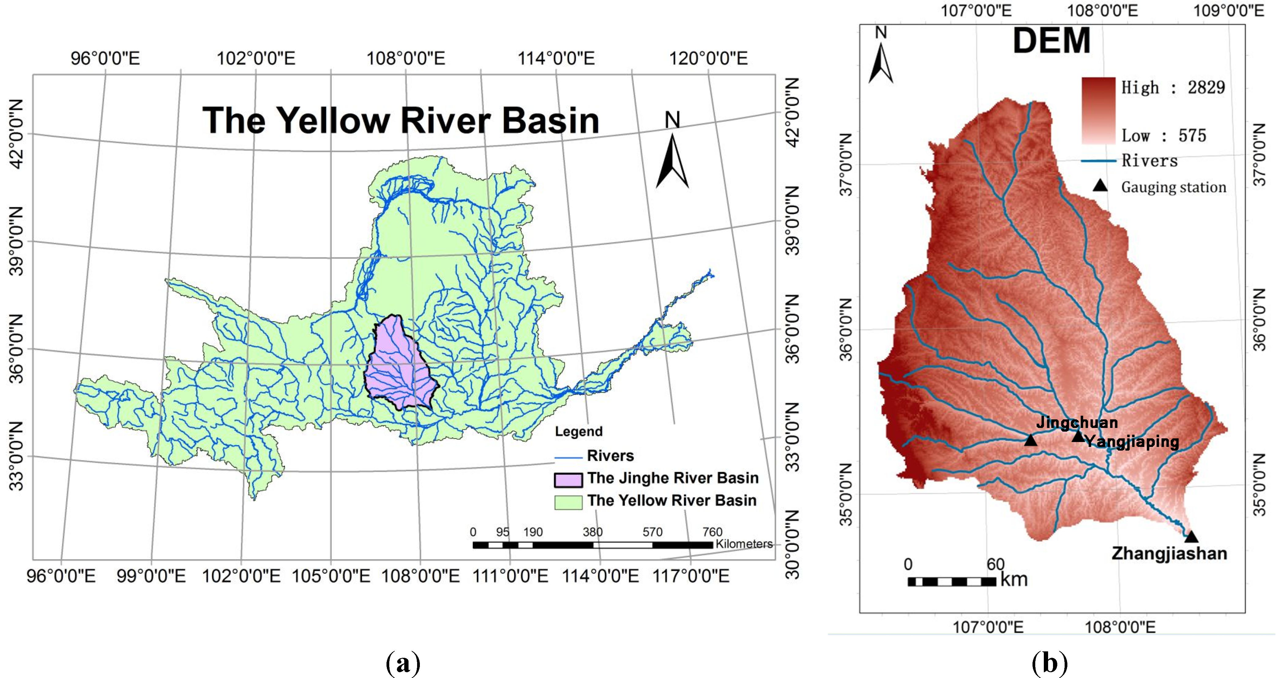
2.1. Site Description

The Jinghe River is a 455-km long tributary of the Yellow River. The Jinghe basin (area of 45,421 km²) is located in the middle of the Loess Plateau (106°20′ E–108°48′ E, 34°24′ N–37°48′ N), and 4.3% of the area is mountainous, 41.7% is loess tableland and broken plateau areas, and 48.8% is loess hilly and gully regions (Figure 1). The basin has deep layers (50–80 m) of loess, composed mainly of fine sand, silt and clay, with silt accounting for up to 50%. The loess has high porosity and is prone to landslides. This basin is one of the most highly eroded areas of the Loess Plateau.

Land use types within the basin include farm land (41.6%), forest (10.2%), grassland (46.5%), water (0.4%), bare land (0.1%), and residential and industrial land (1.31%). The natural vegetation of the basin is of a temperate forest-steppe transition type. Due to historical development processes, human activities have destroyed much of the forest, and now degraded grassland covers most of the area. The growing season of the vegetation is between April and October.

The basin spans seven cities in the provinces of Ningxia, Gansu and Shanxi. There are approximately 6 million people living in the middle and downstream portions of the basin. Water scarcity and soil desertification have resulted in small levels of agriculture and animal husbandry. The industrial structure of the basin is resource-oriented, with energy, heavy and chemical industries accounting for more than 90% of the total industrial production.

The basin has a typical continental climate and is located between the semi-humid and semi-arid temperate zones. It is dry in winter and spring, and storms are frequent in summer and autumn. The average air temperature is 8 °C. Annual precipitation ranges between 350 and 600 mm, with substantial inter-annual variation. Summer precipitation accounts for more than 50% of annual precipitation. Both temperature and precipitation decrease from south to north within the basin.

Figure 1. Digital map of the study area. (a): The yellow river basin; (b): DEM.

Figure 1. Digital map of the study area. (a): The yellow river basin; (b): DEM.

2.2. RHESSys Model

The Regional Hydro-Ecological Simulation System (RHESSys) is a biophysically based eco-hydrological watershed-scale model used to simulate water, carbon and nitrogen cycling and transport. RHESSys represents watersheds as a spatially nested hierarchical structure with a range of meteorological, hydrological and ecological processes associated with different levels of hierarchy [21]. Most vertical hydro-ecological processes are computed in the finest spatial resolution objects, patches and strata, where strata are vertical vegetation layers above the patch. Meteorological inputs and incoming radiation are organized with zones and drainage between patches organized within hillslopes that drain to stream reaches. All of the spatial resolution objects (patches, strata, zones and hillslopes) are generated in a Geographic Information System (GIS)-Geographic Resources Analysis Support System (GRASS-GIS).

The simulation of hydrological processes in RHESSys reflects water storage and transport vertically between the surface canopy/litter and subsurface soil layers and laterally between the simulation units. The soil profile is a simple three-layer soil, including a rooting zone, an unsaturated layer and a saturated layer. RHESSys also calculates storage and evaporation in litter, surface depressions, canopies and snow, and transpiration from overstory and understory canopies. The ecosystem carbon and nitrogen simulation process of RHESSys includes estimates of canopy photosynthesis, respiration and the allocation of net primary productivity to growth, plant turnover, and soil organic matter accumulation and decomposition.

RHESSys has been used for a wide variety of hydrological and ecosystem biogeochemical cycling applications [22,23,24,25,26]. A full description of the RHESSys process representation is given in [21].

2.3. Model Modification

Previous applications of the RHESSys model have focused on small watersheds (<1000 km²) [21,27,28,29]. Several improvements were made to the model in order to apply RHESSys in the Jinghe River Basin, which include in-stream routing, reservoir operation, approaches to parameterize SWCE and a landscape partitioning strategy that supported computational efficiency while maintaining the representation of key components of landscape heterogeneity.

2.3.1. In-Stream Routing

Previous versions of RHESSys assume that any water entering a stream reach leaves the basin within a daily time step. For larger basins, such as the Jinghe River basin, travel time within the stream may exceed one day. To resolve this limitation issue, a nonlinear kinematic wave stream routing module was added to RHESSys. The kinematic wave model is defined by a continuity equation, momentum equation and Manning equation [30]. The numerical solution scheme—Newton’s method—is used to solve these equations.

Continuity:

$$\frac{\partial Q}{\partial x}+\frac{\partial A}{\partial t}=q$$

(1)

Momentum:

$$S_0=S_f$$

(2)

Manning Equation:

$$Q=\frac{1.49}{n}{R}^{\raisebox{1ex}{$2$}\!\left/ \!\raisebox{-1ex}{$3$}\right.}·{S_0}^{\raisebox{1ex}{$1$}\!\left/ \!\raisebox{-1ex}{$2$}\right.}$$

(3)

where $Q$ is the flow rate, $A$ is the cross area of the stream, $q$ is the lateral input, $x$ is the stream length, $t$ is the time interval, $S_0$ is the gravity force term, $S_f$ is the friction force term, $R$ is the hydraulic radius, and $n$ is the Manning coefficient.

Inputs required by the stream routing model include the parameters listed in Table 1 and the stream network topology (e.g., identification of upstream and downstream reaches for each reach). A GRASS-GIS [31] program was developed to automatically construct a table that organizes the stream routing information as RHESSys inputs. This GRASS-GIS program requires spatial raster data to define the stream network, stream cross section information (top width, bottom width and height), Manning roughness and patches. The patch is the smallest spatial modeling unit in RHESSys.

The stream routing sub-model is triggered at the end of each time step (hourly or daily). Any lateral flow (surface or subsurface) from a RHESSys patch containing a stream is included in the stream routing. All improvements to RHESSys in this paper are available on the RHESSys github site. Version 5.14.8 was used for this paper.

Table 1. The format of the stream routing information table.

Item	Information
Overall reaches	Number of stream reaches
Reach	Reach ID, bottom width, top width, max height, slope, Manning roughness, length, Numbers of intersecting units, Numbers of upstream reaches, Number of downstream reaches
Intersecting unit	Patch ID, Zone ID, Hill ID
Upstream reach	Reach ID
Downstream reach	Reach ID

Table 1. The format of the stream routing information table.

Item	Information
Overall reaches	Number of stream reaches
Reach	Reach ID, bottom width, top width, max height, slope, Manning roughness, length, Numbers of intersecting units, Numbers of upstream reaches, Number of downstream reaches
Intersecting unit	Patch ID, Zone ID, Hill ID
Upstream reach	Reach ID
Downstream reach	Reach ID

2.3.2. Reservoirs Sub-Model

To calculate the reservoir impacts on flow, a simple reservoir operation sub-model was added to RHESSys, which is called by the in-stream routing model introduced above. The reservoir operation sub-model is based on user-supplied monthly maximum volume requirements and minimum monthly outflow requirements of reservoirs. The outflow of the reservoir is computed as follows:

$$Q_{out}=\{\begin{array}{c}\begin{array}{cc}{Q}_{min} & Q_{in}-Q_{min}+V<V_{max}\end{array}\\ \begin{array}{cc}{Q}_{in}+V-V_{max}& Q_{in}-Q_{min}+V>V_{max}\end{array}\end{array}$$

(4)

where $Q_{out}$ is the outflow of the reservoir, $Q_{min}$ is the required minimum outflow, V is the storage of the reservoir at the beginning of the time step, $V_{max}$ is the storage capability of the reservoir for one month, and $Q_{in}$ is the inflow of the reservoir. The outflow of the reservoir must satisfy the requirement of the minimum outflow requirement first, followed by the monthly volume limitation. User-prescribed human water use is subtracted from the reservoir volume. A reservoir information input file was added to the RHESSys input files, which records the operation information of each reservoir.

2.3.3. SWCE

In this study, two kinds of SWCE were included in the simulation: terrace land and check dams. The impacts of terrace land are simulated based on the ratio terrace land area to the total area for each patch, where patches are the fine-scale simulation unit in the model (average patch size is 1 km²). These ratios are calculated from the terrace land area data available at the county scale from the water conservancy statistical yearbooks of each county. An increased surface detention storage capacity is used in the RHESSys model as a parameter to define the impact of terraced land on runoff. The relationship between terrace land ratio and detention storage capacity was based on the literature [32]. A reduced slope associated with terraced land is also implicitly included through the use of slope in the RHESSys subsurface and surface routing computation.

The hydrological impacts of check dams are simulated at the hillslope scale (e.g., area draining either side of a stream reach). Information on the annual new check dam deposition area of every county is available from water conservancy statistical yearbooks. To estimate the number of check dams in a hillslope, this annual new check dam deposition area was divided by the mean annual deposition area of one check dam. The mean annual deposition area of a typical check dam was 0.0029 km² and the drainage area of one check dam was 1.04 km² according to local survey data. Hillslope-scale runoff generated within the drainage area is assumed to be the inflow of the check dam. Check dams are simulated using the reservoir sub-model described above, assuming Q_min to be zero. Thus, the check dam is assumed be an overflow dam with a maximum storage (160,000 m³). The surface evaporation of water stored in the check dam is calculated using the Penman Method. The water surface area is computed as follows:

$$A_{water}=\sqrt{2VB/i}$$

(5)

where $V$ is the reservior storage, m³; $B$ is the reservior width, m; $i$ is the bottom slope.

RHESSys allows the user to change the spatial resolution and shape of the modeling units [10]. It needs to consider both computational efficiency and spatial resolution in spatial units partitioning. Based on a preliminary simulation to evaluate changes in streamflow with resolution, patches were based on a 1-km resolution Digital Elevation Map (DEM). The hillslope was partitioned by GRASS-GIS watershed generation, with a threshold drainage area of 100 km². The basin was created by the GRASS-GIS basin boundary program based on the outlet hydrological measurement station in the Jinghe River Basin.

2.4. Data

Meteorological data collected from 8 climate stations and 13 precipitation stations were used to generate climate data input for each zone (RHESSys meteorology spatial object). Spatial patterns were generated through interpolation using a standard Theissen polygon approach. Meteorological data were retrieved from the China Meteorological Data Sharing Service System, including daily precipitation, maximum, minimum, and mean daily air temperature from 1956 to 2010. Daily precipitation data from 1956 to 2010 were obtained from the Yellow River Water Conservancy Commission (YRWCC). YRWCC also provided monthly stream flow data from the Zhangjiashan hydrological station, which is located at the outlet of the Jinger River Basin.

The 30 Arc-Second DEM data were retrieved from the website of the U.S. Geological Survey (USGS) [33]. Slope, aspect, stream and basin boundaries were created based on these DEM data in GRASS-GIS. Soil type and characters were obtained from the National Second Soil Survey Data and Soil Types of China.

Land use/cover data for 1980, 1985, 1997, 2000 and 2005 (scale 1:100,000) were used in the model, which were derived from Landsat TM data and revised with survey data of land use in the yearly reports from administrative districts. Land use was reclassified into 3 categories: undeveloped, urban and agriculture land. Undeveloped land includes forest, grassland and wasteland. In the agriculture land, irrigation and fertilization input are included. The input values for irrigation and fertilization are 0.1 m³ water/m²/year and 16.05 g NH₄/m²/year according to local survey data. The vegetation type map was also obtained from the land use/cover data with categories of forest, grass and crop.

The stream cross-section data (bottom width, top width, depth, Manning roughness) for the main stream were available from 13 hydrological stations. For the upstream reach, bottom width, top width, and depth were calculated based on the relationship between the drainage area and cross section [32], and Manning roughness was calculated using the method in reference [34]. Reservoir operation information was obtained from water resource survey data. Human water use data were obtained from the Second Countrywide Comprehensive Water Resources Planning in China. SWCE information was obtained from the water conservancy statistical yearbooks of each county.

Net Primary Production Yearly L4 Global 1-km products and Leaf Area Index—Fraction of Photosynthetically Active Radiation 8-Day L4 Global 1-km products of the Moderate Resolution Imaging Spectroradiometer (MODIS) were retrieved from U.S. Geological Survey (USGS) website, maintained by the Land Processes Distributed Active Archive Center (LP DAAC) of the National Aeronautics and Space Administration (NASA) at the USGS/Earth Resources Observation and Science (EROS) Center, Sioux Falls, South Dakota, 2011.

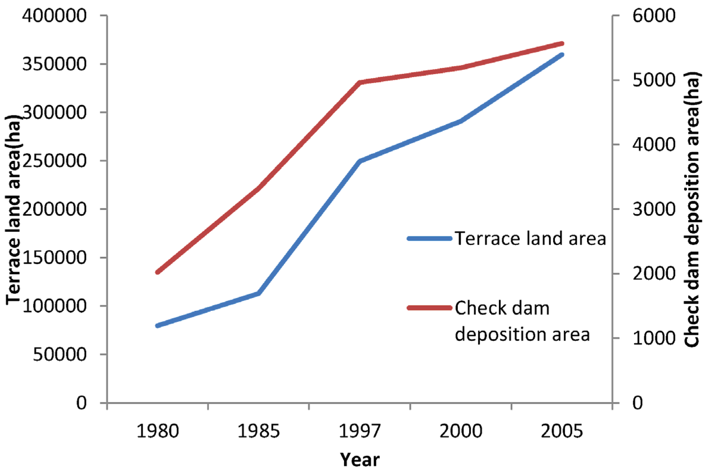
2.5. Soil and Water Conservation Measures

The soil and water conservation measures included in the model can be divided into two types: vegetation restoration and SWCE. Vegetation restoration is defined by changes in vegetation type (forest, grass and farmland), which are obtained from remote sensing data. The vegetation type would be updated based on Landsat TM data of 1980, 1985, 1997, 2000 and 2005. These updates were used to reflect vegetation changes that occurred as a result of restoration measures. The RHESSys vegetation growth model was used to calculate vegetation biomass and associated characteristics such as leaf area index and net primary productivity. The ratios of the vegetation area in the whole basin are shown in Figure 2.

Figure 2. The ratio of the vegetation area in whole basin.

Figure 2. The ratio of the vegetation area in whole basin.

With the approaches for SWCE simulation described in Section 2.3, two kinds of SWCE were included in the simulation: terrace land and check dams. Terrace land and check dams were obtained from water conservancy statistical yearbooks of each county in the basin, which were updated for years 1980, 1985, 1997, 2000 and 2005. Figure 3 shows the terrace land area and check dam control area for the whole basin. The terrace land area ratio in each county was used to generate a raster map of the terrace land ratio for all patches. The ratio of terrace land was divided into 6 categories to match different detention storage capacity parameters (Table 2). The annual new check dam deposition area ratios were calculated in each county and the result was written into a raster file.

Figure 3. Total terrace land area and check dam control area of the basin.

Figure 3. Total terrace land area and check dam control area of the basin.

Table 2. Relationship between detention storage capacity and terrace land area ratio of the whole area.

Categories	1	2	3	4	5	6
Terrace land area ratio	<0.04	0.04–0.06	0.06–0.08	0.08–0.12	0.12–0.2	0.25
Detention storage capacity (m)	0.005	0.0065	0.009	0.0125	0.02	0.03

Table 2. Relationship between detention storage capacity and terrace land area ratio of the whole area.

Categories	1	2	3	4	5	6
Terrace land area ratio	<0.04	0.04–0.06	0.06–0.08	0.08–0.12	0.12–0.2	0.25
Detention storage capacity (m)	0.005	0.0065	0.009	0.0125	0.02	0.03

2.6. Model Parameterization and Calibration

Vegetation parameters are available from the RHESSys parameter database and literature [35]. Some of the parameters were modified based on previous field work in the basin [36].

Drainage parameters are mostly obtained from the RHESSys parameter database, which links these parameters with soil texture. Soil depth, grading composition and porosity were obtained from the National Second Soil Survey Data. These parameters are linked to the classification and are distributed spatially according to the 1:10,000,000 soil classification map in China [32]. Calibrated drainage parameters include: saturated hydraulic conductivity (K), decay of saturated hydraulic conductivity with depth (m), pore size index (pore_size_index), air entry pressure (psi_air_entry), percentage of infiltrated water that percolates to the deeper groundwater store (gw1), and drainage rate of the deep groundwater store (gw2).

A spin-up RHESSys simulation of 2200 years was run prior to calibration and model analysis to stabilize the soil carbon and nitrogen pools. Fifty-four years of climate data (1957–2010) were repeated to create weather sequences for this spin-up run. Following spin-up, drainage parameters in the model were calibrated by comparing observed and modeled streamflow. A Monte Carlo approach was used to sample parameter sets of m, K, pore_size_index, psi_air_entry, gw1 and gw2 values. By comparing observed and simulated streamflow, an acceptable parameter set was selected to use in the model analysis. The calibrations included 250 simulations of a 5-year period, 1991–1995. The performance metrics used to evaluate the model performance include the error in mean annual streamflow estimates and the Nash-Sutcliffe efficiency (NSE) [37] between observed and simulated monthly streamflow of the Zhangjiashan gauging station. The parameter set selected from the calibration was able to capture major hydrologic trends, based on the Nash–Sutcliffe efficiency for monthly streamflow (0.74) (Figure 4). The error in estimating mean monthly streamflow for the calibration period was 9.2%.

Figure 4. Calibration results of monthly discharge at the Zhangjiashan gauging station.

Figure 4. Calibration results of monthly discharge at the Zhangjiashan gauging station.

2.7. Model Verification Method

The model verification includes two parts: hydrological verification and ecological verification. In the hydrological verification, a single parameter set based on the performance metrics outlined in the calibration was selected and used for subsequent model validation. The global parameter uncertainty analysis, such as Generalized Likelihood Uncertainty Estimation (GLUE), is not included in this study because it is too computationally intensive in such a large basin running at relatively fine scales. In ecological verification, RHESSys estimations of net primary productivity (NPP) and leaf area index LAI were compared with Moderate Resolution Imaging Radiometer (MODIS) NPP and LAI products. Specifically, RHESSys estimates of annual average NPP for the years 2000–2010, and LAI distribution for 22 August 2009 were compared with MODIS NPP and LAI products. The basin mean values of the MODIS NPP products were calculated in ArcGIS software.

2.8. Model Scenarios

To evaluate the SWC impacts on streamflow, several different RHESSys model scenarios were compared, which separate the vegetation changes and SWCE (terrace land and check dams) impacts. Three scenarios were simulated in the simulation from 1980 to 2010: Scenario 1 had no prescribed vegetation changes (vegetation area and vegetation types are kept the same as 1980; however, vegetation changes associated with climate variation that are simulated by the model were included), and also assumed no new SWCE following 1980; Scenario 2 prescribed vegetation changes using the actual vegetation data from remote sensing-based land use/cover but did not include new SWCE; Scenario 3 included both prescribed vegetation changes and conservation practices based on SWCE data, which are the closest to historical simulations. Thus, the streamflow differences between scenario 1 and scenario 2 illustrate the impacts from vegetation management, while the difference between scenario 2 and scenario 3 illustrate the additional impacts associated with SWCE.

To isolate other influences of streamflow, the climate and human water use data were the same in the three scenarios. The data were the actual historical data as described above. Therefore, differences in model estimates between the 3 scenarios can be attributed to the impact of management practices on streamflow. The results of the scenario analysis were used to estimate the impact of SWCE, vegetation change and their combination on streamflow.

3. Results and Discussion

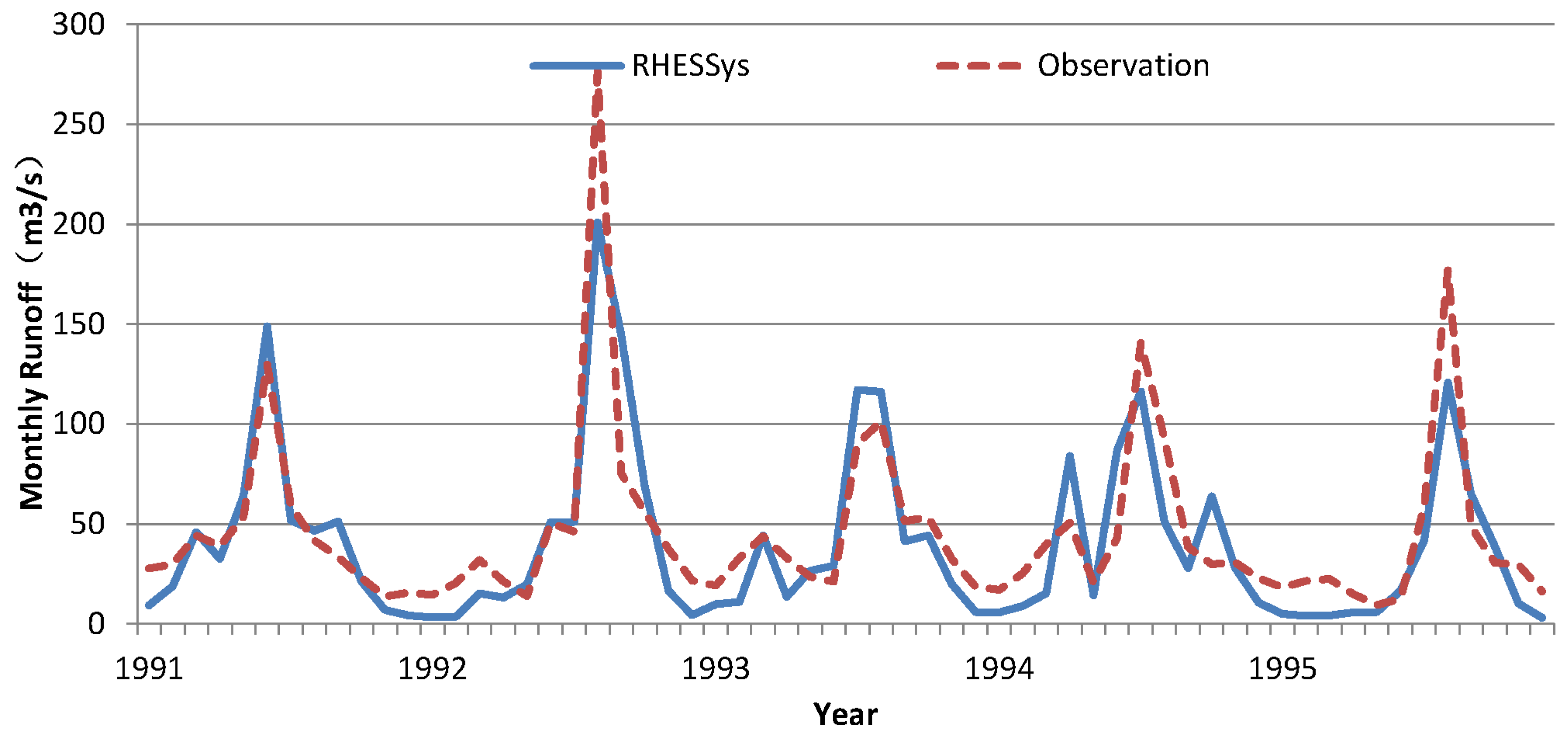
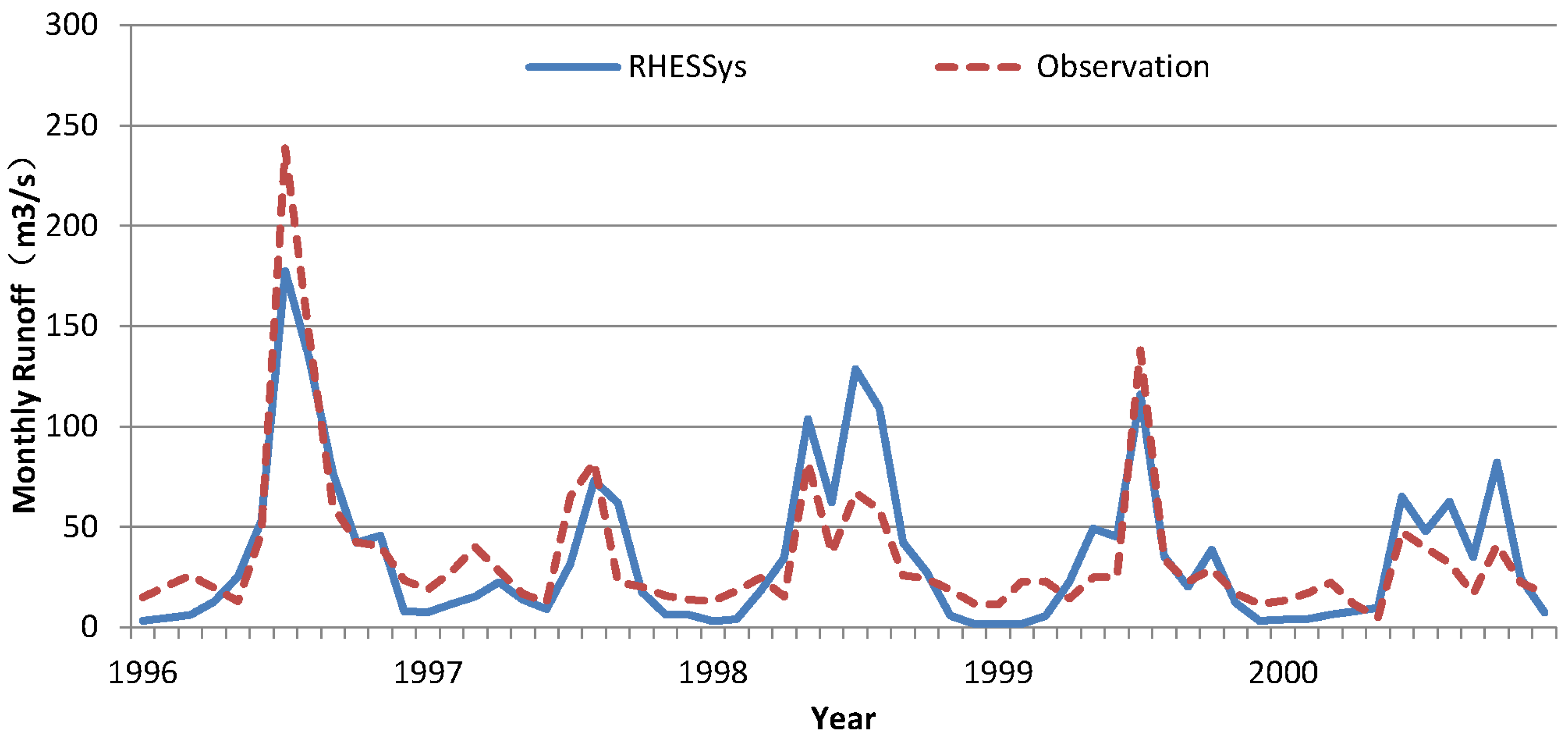
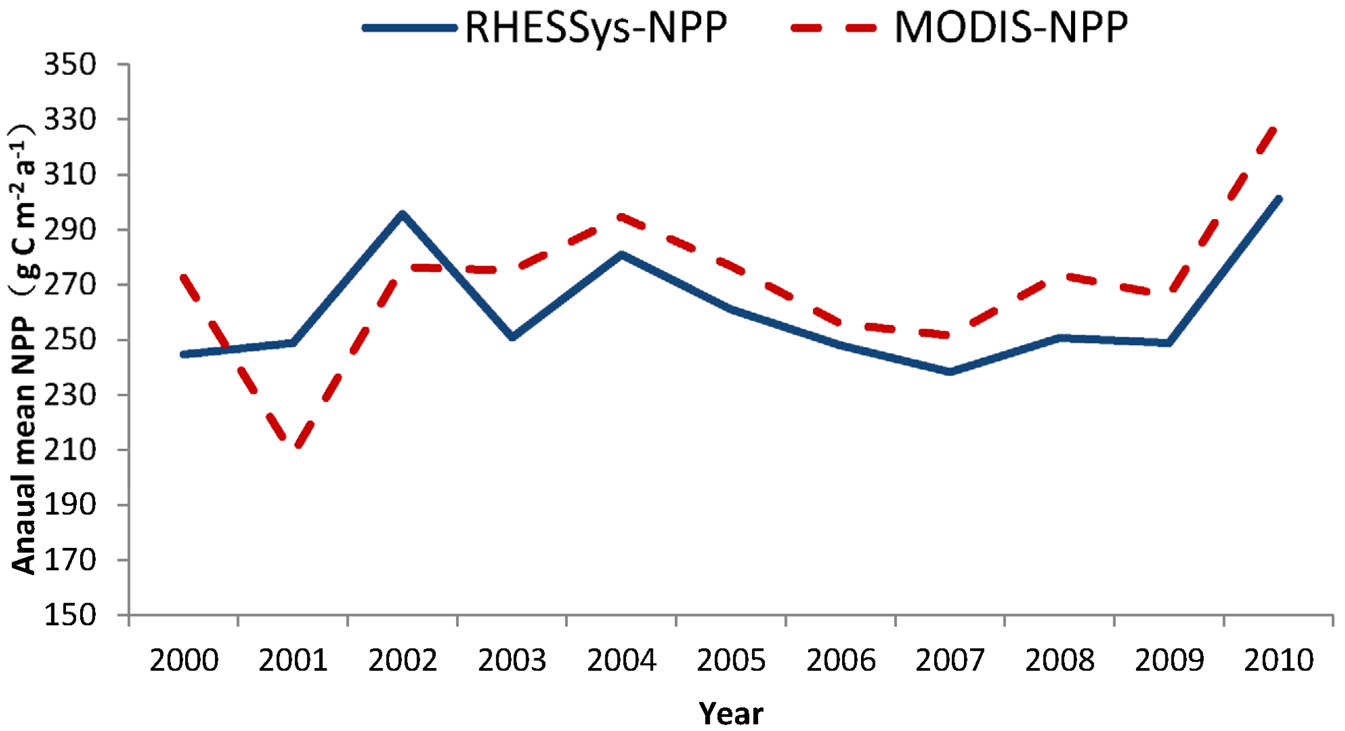
3.1. Model Verification

Monthly streamflow data from 1996 to 2000 were used for validation. For the validation period, simulated mean annual streamflow differed from observed values by only 0.4% and the Nash-Sutcliffe Efficiency was 0.70 for monthly streamflow (Figure 5). These results suggested that the model did a reasonable job of capturing the major hydrological processes.

Figure 5. Verification results of monthly discharge at the Zhangjiashan gauging station.

Figure 5. Verification results of monthly discharge at the Zhangjiashan gauging station.

The model estimates of annual average NPP for the years 2000–2010 were compared with Terra/MODIS Net Primary Production Yearly L4 Global 1-km products. The NPP results of RHESSys matched well with those derived from the MODIS products (Figure 6) (mean error is less than 5%). Model estimates of spatial distribution of LAI for 20 August 2009 were compared with Terra/MODIS Leaf Area Index—Fraction of Photosynthetically Active Radiation 8-Day L4 Global 1-km products. The LAI estimates from RHESSys are similar to the MODIS products: MODIS LAI ranges from 0 to 6.8; RHESSys LAI from 0 to 7.7. Spatial patterns are also similar (Figure 7), although the MODIS product showed a greater spatial variation in LAI than the RHESSys. These simulations using the RHESSSys spatial resolution were often coarser than the resolution of the MODIS products.

Figure 6. Comparison of annual mean NPP of the Jinghe River Basin from the RHESSys results and MODIS products.

Figure 6. Comparison of annual mean NPP of the Jinghe River Basin from the RHESSys results and MODIS products.

Figure 7. Comparison of LAI distribution between the MODIS products (a) and RHESSys results (b) on 20 August 2009.

Figure 7. Comparison of LAI distribution between the MODIS products (a) and RHESSys results (b) on 20 August 2009.

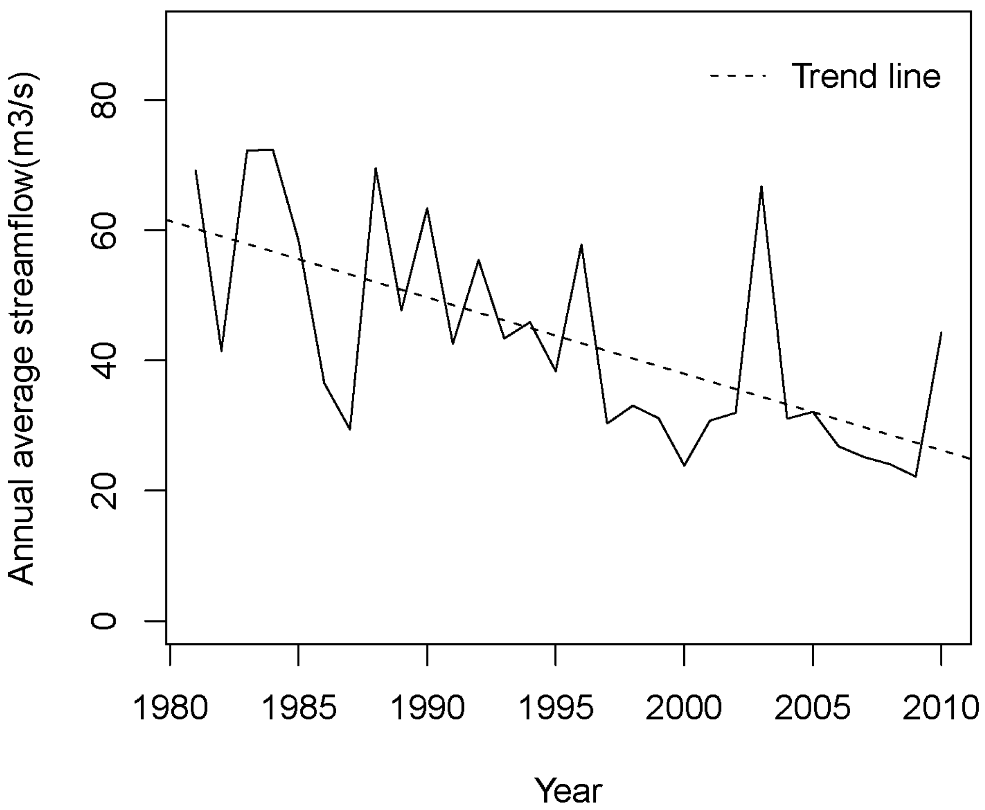
3.2. Streamflow Decrease and Other Impacts

Before the analysis of SWC impacts on streamflow, the streamflow change in the recent decades was evaluated. The Mann-Kendall trend test was used to evaluate the temporal trend of annual mean streamflow at the Zhangjiashan gauging station. The results showed that annual mean streamflow decreased from 1980 to 2010 with a significant change trend of 0.80 m³/s per year (with 95% confidence interval, Figure 8).

Figure 8. Annual mean discharge of the Jinghe River (Zhangjiashan gauging station) and its change trend.

Figure 8. Annual mean discharge of the Jinghe River (Zhangjiashan gauging station) and its change trend.

The climate change trends of the Jinghe River Basin in the recent decades were evaluated. The Mann-Kendall trend test was used to evaluate the change trend of annual precipitation. The results showed that the annual precipitation from 1980 to 2010 has a non-significant change trend. The Mann-Kendall trend test was also used to analyze the annual mean value of daily maximum and minimum temperature, which both showed a significant increasing trend of 0.7 °C/decade from 1980 to 2010 with a 95% confidence coefficient. The temperature increase may cause evapotranspiration (ET) increases; however, ET has a non-significant change trend. The impacts of climate are difficult to evaluate. The human water use increased significantly from the 1980s to 2000s. The annual human water use ranged from 0.38 to 0.66 billion m³. To isolate this impact on streamflow, Scenario 1 was used in the simulation.

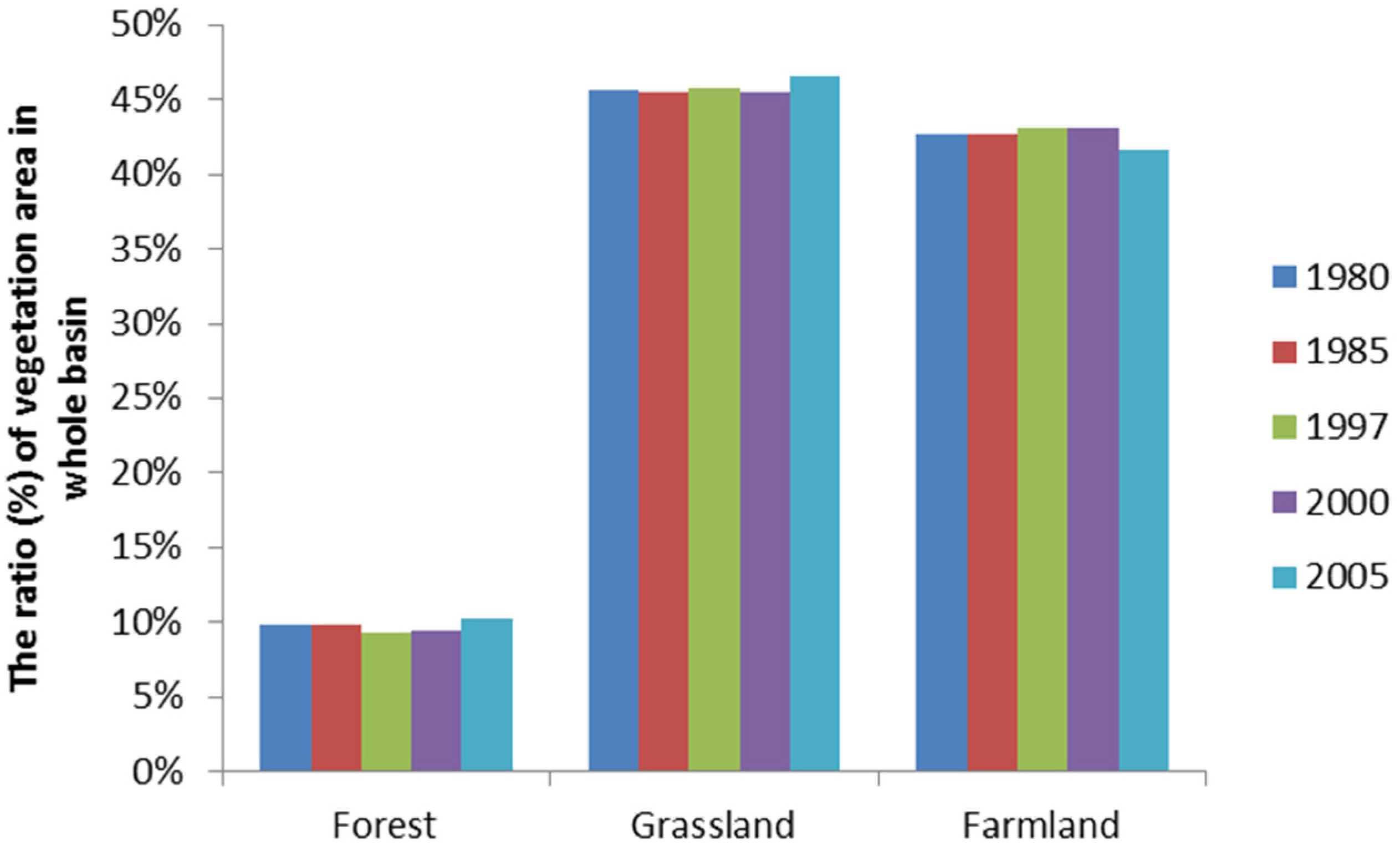
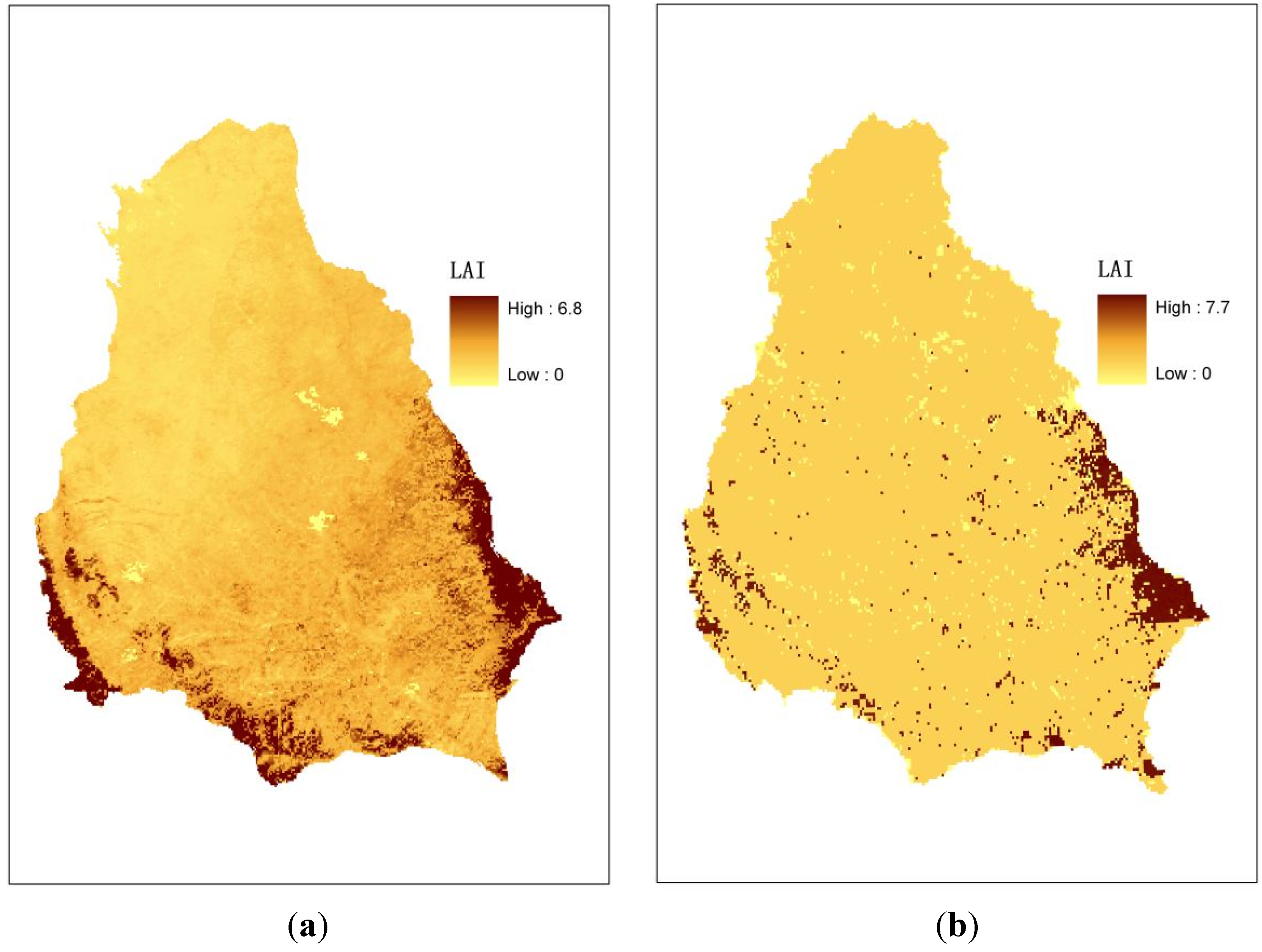
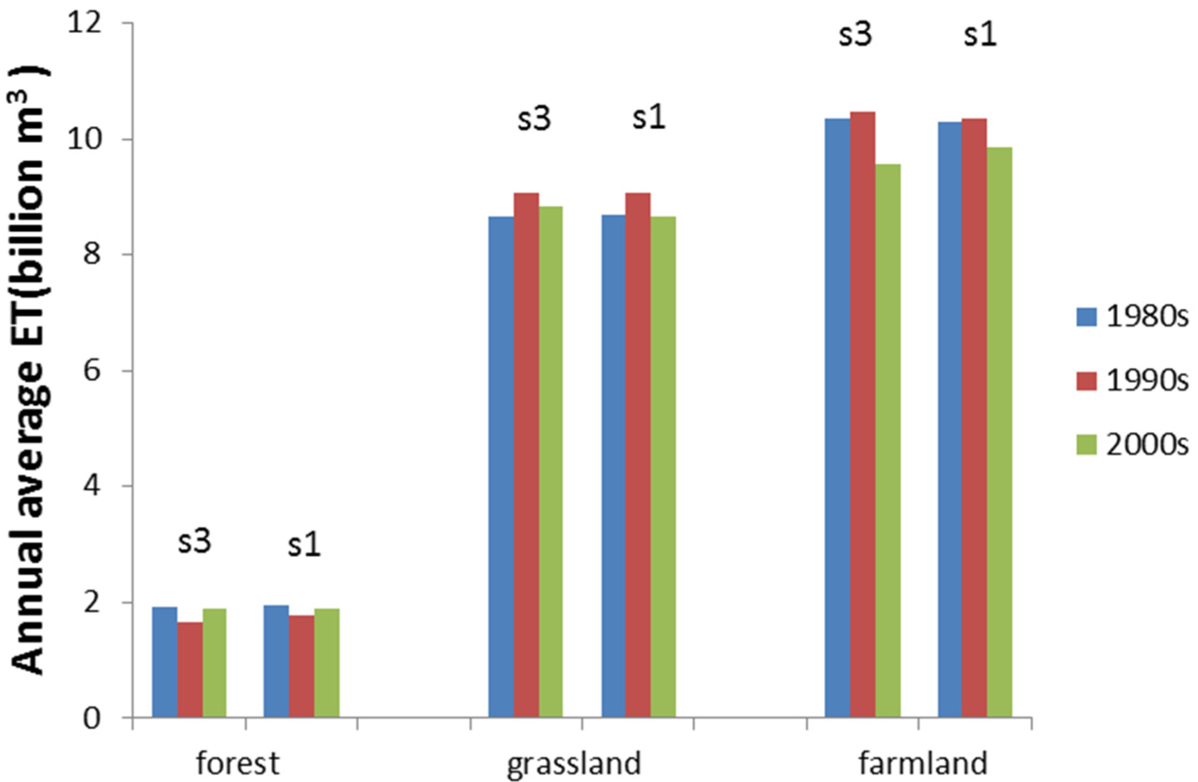
3.3. Impacts of Vegetation Changes

First, analysis was performed for the changes in vegetation type and the associated ET of vegetation patches in the recent decades from scenario 3 (historical simulation). According to Figure 2, the forest area decreased in the 1990s compared with the 1980s, and then increased in 2005. Grassland area changed little from the 1980s to the 1990s, and then increased in 2005. Farmland increase in the 1990s compared with the 1980s, and then decreased in 2005. These results demonstrated that the impact of efforts to recover natural vegetation and reclamation both happened in the 1990s, and there is some evidence of a turning point around 2000 after which the natural vegetation (forest and grassland) started to increase and the farmland started to decrease.

The vegetation area changes suggested that some forest areas and grasslands were destroyed in the 1990s. Farmland increases in the 1990s imply that some forest areas and grasslands became farmland. But there is a turning point around 2000, when the area of forest and grassland increased and farmland decreased. In 1999, a state-funded project, “Grain for Green” was launched in western China for soil erosion control and vegetation improvement by converting slope cropland into grassland or forest [2]. The analysis of land cover data implied that this project had a small but visible impact on vegetation patterns, specifically an increase in forest.

The estimated total ET of the vegetation patches was averaged by decade (Figure 9), and the results showed that in scenario 3, the ET in the 1990s was the highest (21.2 billion m³), followed by the 1980s (20.9 billion m³), whereas the ET in the 2000s was the lowest (20.3 billion m³). Similarly, the ET of farmland in the 1990s is the largest, followed by the 1980s, but lowest in the 2000s. The ET of grassland in the 1990s is the largest, followed by the 1980s, and the ET of grassland in the 2000s was the lowest. The ET of forest in the 1980s is the largest, followed by the 2000s, and the ET of forest in the 1990s was the lowest. The ET results of scenario 1 showed the change trends were similar to scenario 3, but with differences (Figure 9).

The ET of vegetation patches in scenario 3 reflected changes in the distribution of land cover type between forest, grassland and farm land. A comparison between results of scenario 3 and scenario 1 shows the combined impact of SWC measures (Figure 9). The forest area decreased in the 1990s and increased after 2000, as did the contribution of forest ET in scenario 3. The ET of farmland increased in the 1990s and decreased in the 2000s in scenario 3, which is the same trend as the farmland area change. The differences between scenario 3 and scenario 1 reinforce this argument. The only disagreement between ET and the vegetation area change trend was the grassland in the 2000s in scenario 3. The grassland area increased in the 2000s, but the contribution of ET from grassland decreased in the 2000s. Since soil and other factors were constant in the model, this suggests that climate differences played an important role. The contribution of ET from grassland in scenario 3 was larger than that in scenario 1 in the 2000s, which showed the grassland area increase caused the ET increase. All of the results demonstrate the vegetation area influences the ET. Although they had the lowest rainfall in the 1990s, the total ET of the vegetation patches was the highest. The total ET of the vegetation patches increased in the 1990s and decreased in the 2000s.

Figure 9. The ET of every vegetation type in scenario 3.

Figure 9. The ET of every vegetation type in scenario 3.

Streamflow in every decade was compared across the 3 scenarios (Figure 10). Scenario 1 is the baseline simulation with no vegetation change or SWCE included (e.g., vegetation from 1980 was used). Vegetation type change was included in scenario 2. Therefore, the streamflow differences between scenario 1 and scenario 2 were the streamflow changes caused by the vegetation changes. The streamflow results show that the vegetation change from the 1980s to the 2000s decreased the annual average streamflow by about 0.027 billion m³ (1.8%). The annual average decrease is 0.002 billion m³ in the 1980s (0.1%), 0.043 billion m³ in the 1990s (3.3%), and 0.036 billion m³ in the 2000s (2.7%, Table 3).

Figure 10. Simulated annual average streamflow of the Jinghe River in every decade.

Figure 10. Simulated annual average streamflow of the Jinghe River in every decade.

Table 3. Annual average streamflow simulation results and SWC impacts on annual average streamflow (unit: billion m³).

Item	1981–1990	1991–2000	2001–2010	1981–2010
Vegetation change impacts (Scenario 1–Scenario 2)	0.002 (0.1%)	0.043 (3.3%)	0.036 (2.7%)	0.027 (1.8%)
SWCE impacts (Scenario 2–Scenario 3)	0.132 (7.3%)	0.054 (4.2%)	0.100 (7.7%)	0.095 (6.5%)
Total SWC impacts (Scenario 1–Scenario 3)	0.134 (7.4%)	0.097 (7.5%)	0.136 (10.4%)	0.122 (8.3%)

Table 3. Annual average streamflow simulation results and SWC impacts on annual average streamflow (unit: billion m³).

Item	1981–1990	1991–2000	2001–2010	1981–2010
Vegetation change impacts (Scenario 1–Scenario 2)	0.002 (0.1%)	0.043 (3.3%)	0.036 (2.7%)	0.027 (1.8%)
SWCE impacts (Scenario 2–Scenario 3)	0.132 (7.3%)	0.054 (4.2%)	0.100 (7.7%)	0.095 (6.5%)
Total SWC impacts (Scenario 1–Scenario 3)	0.134 (7.4%)	0.097 (7.5%)	0.136 (10.4%)	0.122 (8.3%)

The results showed that the vegetation changes from 1980 led to a small streamflow decrease. In addition to the recovery of vegetation resulting from SWC, other activities like farmland increase could also result in vegetation changes, which means that vegetation recovery from SWC is not the only reason for the streamflow change discussed above. It is difficult to distinguish the vegetation recovery from SWC from other vegetation changes in the vegetation map. Future studies may focus on the impacts of vegetation recovery from SWC only when better methods of distinguishing vegetation recovery have been found.

3.4. SWCE Impacts

The SWCE including the terrace land and check dams had more substantial impacts on streamflow estimates. The survey data from water conservancy statistical yearbooks of each county showed that the area of the terrace land and check dams increased dramatically in the past decades.

The streamflow changes caused by SWCE were calculated by scenario analysis using our eco-hydrological model. The estimated streamflow differences between scenario 2 and scenario 3 are streamflow changes caused by SWCE. The simulated streamflow shows that SWCE decreased annual streamflow by 0.095 billion m³ (6.5%). The annual decrease is 0.132 billion m³ in the 1980s (7.3%), 0.054 billion m³ in the 1990s (4.2%), and 0.100 billion m³ in the 2000s (7.7%, Table 3).

These results showed that SWCE rather than vegetation changes were likely to be the greater source of reduced streamflow. Further differences between scenario 2 and 3 showed only the impact of SWCE, since other input data were the same for both scenarios. The substantially greater streamflow reductions in scenario 3 therefore reflect SWCE rather than vegetation changes. These results highlight how the combination of check dams and terrace land could increase ET losses and infiltration associated with a larger detention storage capacity. Similarly, the check dams could block the streamflow and increase the water storage in the stream reaches and the associated ET losses. Field measurements in the Loess Plateau showed that the terrace land can reduce 73.5%–94.5% of the surface runoff [38] at a hillslope scale. In the larger-scale study, these local scale reductions translate into a basin-wide reduction of close to 8% (for the 2000s).

3.5. Integrated Impacts

Since scenario 3 includes both components of SWC (vegetation change and engineered structures) while scenario 1 included neither, the differences between them are the impacts of both soil and conservation measurements. The model results showed that the soil and conservation decreased annual streamflow by 0.122 billion m³, which is 8.3% of the annual streamflow of scenario 1. The annual decrease was 0.134 billion m³ in the 1980s, 0.097 billion m³ in the 1990s, and 0.136 billion m³ in the 2000s, which are 7.4%, 7.5% and 10.4% of the annual streamflow of scenario 1, respectively (Table 3). The largest impacts occurred in the 2000s, suggesting that the SWC measures after 1999 aggravated the impacts on streamflow. These results were consistent with the shifts in SWC policy during the same period.

The SWCE had larger impacts on streamflow than the vegetation changes. The SWCE decreased annual streamflow by 0.095 billion m³ from 1981 to 2010, which accounts for 78% of the total impacts (Table 3). The vegetation change decreased annual streamflow by 0.027 billion m³ from 1981 to 2010 and accounts for 22% of the total impacts. These results suggested that efforts to reduce the impacts of soil and water conservation on streamflow in this region should focus on the design of SWCE (check dams and terraces) to reduce evaporative losses rather than on vegetation changes.

Streamflow in scenario 1, which isolated the impact of climate and human water use, also changed with time. There was a substantial decline in streamflow (27%) between the 1980s and 2000s. The magnitude of the impact of climate and human water use on streamflow is greater than the impact of SWCE and the vegetation change. Scenarios 2 and 3 demonstrated that the effects of SWCE and vegetation change were in the same direction (declines in streamflow) and thus aggravated the impacts of climate and human water use.

Although this model-based study confirmed that SWC is likely responsible for declines in annual streamflow, it is important to acknowledge that SWC has positive impacts on erosion control. Liu et al., [39] found that the sediment in the Jinghe River decreased 12.1% from 1960 to 2000 and attributed this to SWC in this basin. Erosion control and surface water resources always have tradeoffs that must be considered when proposing soil and water conservation measures.

4. Conclusions

This paper presents an application of a biophysically-based eco-hydrological model—Regional Hydro-Ecological Simulation System (RHESSys)—In the Jinghe River Basin to study the impacts of SWC measures including vegetation recovery and engineering construction in the Loess Plateau. Several improvements have been made to the model, including adding in-stream routing and reservoir operation sub-models. Field observation data, literature values and remote sensing data were used to calibrate the model parameters. The hydrological and ecological verifications showed that the model offers a reasonable representation of the eco-hydrological dynamic processes in this basin. Three scenarios were developed to compare the impacts of vegetation changes with SWCE on streamflow at the Jinghe River Basin scale. Scenarios were based on remote sensing and planning documents that summarized SWC deployment over the past 3 decades. Model estimates suggested that SWC decreased annual streamflow by 8.3% (0.122 billion m³/year), with the largest decreases occurring in the 2000s, which is consistent with the intensification of SWC measures after 1999. Engineering changes such as terraces and check dams (SWCE) account for approximately 78% of the total impacts, with the remainder attributed to vegetation recovery. There is also a decline in streamflow associated with climate and human water use, which is accentuated by the impact of SWC. These results suggested that efforts to reduce water loss from SWC should focus on reducing evaporative losses from SWCE rather than vegetation changes. More generally, this study demonstrated the feasibility of applying a mechanistically coupled eco-hydrological model at the scale of the Jinghe River Basin and provided a new tool to support the management of SWC and water resources in the Loess Plateau.

References

1. Shi, H.; Shao, M. Soil and water loss from the Loess Plateau in China. J. Arid Environ. 2000, 45, 9–20. [Google Scholar] [CrossRef]
2. Chen, L.; Wei, W.; Fu, B.; Lü, Y. Soil and water conservation on the Loess Plateau in China: Review and perspective. Prog. Phys. Geogr. 2007, 31, 389–403. [Google Scholar] [CrossRef]
3. Fu, B. Soil erosion and its control in the loess plateau of China. Soil Use Manag. 1989, 5, 76–82. [Google Scholar] [CrossRef]
4. Dou, L.; Huang, M.; Hong, Y. Statistical Assessment of the Impact of Conservation Measures on Streamflow Responses in a Watershed of the Loess Plateau, China. Water Resour. Manag. 2009, 23, 1935–1949. [Google Scholar] [CrossRef]
5. He, X.; Li, Z.; Hao, M.; Tang, K.; Zheng, F. Down-scale analysis for water scarcity in response to soil-water conservation on Loess Plateau of China. Agric. Ecosyst. Environ. 2003, 94, 355–361. [Google Scholar] [CrossRef]
6. Huang, M.; Zhang, L. Hydrological responses to conservation practices in a catchment of the Loess Plateau, China. Hydrol. Process. 2004, 18, 1885–1898. [Google Scholar] [CrossRef]
7. Ran, D.; Liu, B.; Wang, H. Analysis on sediment reduction of the Yellow River through soil and water conservation measures. Soil Water Conserv. China 2002, 10, 35–36. [Google Scholar]
8. Xu, J.; Li, X.; Wang, Z. Analysis on ecological water consumption of soil and water conservation measures in the Loess Plateau. Yellow River 2003, 25, 21–22. [Google Scholar]
9. Wang, Q.; Fan, X.; Qin, Z.; Wang, M. Change trends of temperature and precipitation in the Loess Plateau region of China, 1961–2010. Glob. Planet. Chang. 2012, 92, 138–147. [Google Scholar] [CrossRef]
10. Band, L.E.; Tague, C.L.; Brun, S.E.; Tenenbaum, D.E.; Fernandes, R.A. Modelling Watersheds as Spatial Object Hierarchies: Structure and Dynamics. Trans. GIS 2000, 4, 181–196. [Google Scholar] [CrossRef]
11. He, H.; Zhou, J.; Zhang, W. Modelling the impacts of environmental changes on hydrological regimes in the Hei River Watershed, China. Glob. Planet. Chang. 2008, 61, 175–193. [Google Scholar] [CrossRef]
12. Jaskierniak, D. Modelling the Effects of Forest Regeneration on Streamflow Using Forest Growth Models; University of Tasmania: Hobart, Australia, 2011. [Google Scholar]
13. Li, Z.; Liu, W.; Zhang, X.; Zheng, F. Impacts of land use change and climate variability on hydrology in an agricultural catchment on the Loess Plateau of China. J. Hydrol. 2009, 377, 35–42. [Google Scholar] [CrossRef]
14. O’Loughlin, E.M.; Short, D.L.; Dawes, W.R. Modelling the Hydrological Response of Catchments to Land Use Change. In Proceedings of the Hydrology and Water Resources Symposium 1989: Comparisons in Austral Hydrology, Canberra, Australia, 28–30 November 1989; pp. 335–340.
15. Sun, G.; Zhou, G.; Zhang, Z.; Wei, X.; McNulty, S.G.; Vose, J.M. Potential water yield reduction due to forestation across China. J. Hydrol. 2006, 328, 548–558. [Google Scholar] [CrossRef]
16. Zhang, L.; Dawes, W.R.; Hatton, T.J. Modelling hydrologic processes using a biophysically based model—Application of WAVES to FIFE and HAPEX-MOBILHY. J. Hydrol. 1996, 185, 147–169. [Google Scholar] [CrossRef]
17. Zhang, X.P.; Zhang, L.; McVicar, T.R.; van Niel, T.G.; Li, L.T.; Li, R.; Yang, Q.; Wei, L. Modelling the impact of afforestation on average annual streamflow in the Loess Plateau, China. Hydrol. Process. 2008, 22, 1996–2004. [Google Scholar] [CrossRef]
18. Chapin, F.S., III; Mooney, H.A.; Matson, P. Principles of Terrestrial Ecosystem Ecology; Springer: Berlin, Germany; Heidelberg, Germany, 2002. [Google Scholar]
19. Khurana, E.; Singh, J.S. Ecology of seed and seedling growth for conservation and restoration of tropical dry forest: A review. Environ. Conserv. 2001, 28, 39–52. [Google Scholar] [CrossRef]
20. Sullivan, C.Y.; Eastin, J.D. Plant physiological responses to water stress. Agric. Meteorol. 1974, 14, 113–127. [Google Scholar] [CrossRef]
21. Tague, C.L.; Band, L.E. RHESSys: Regional Hydro-Ecologic Simulation System—An Object-Oriented Approach to Spatially Distributed Modeling of Carbon, Water, and Nutrient Cycling. Earth Interact. 2004, 8, 1–42. [Google Scholar] [CrossRef]
22. Band, L.E.; Tague, C.L.; Groffman, P.; Belt, K. Forest ecosystem processes at the watershed scale: Hydrological and ecological controls of nitrogen export. Hydrol. Process. 2001, 15, 2013–2028. [Google Scholar] [CrossRef]
23. Zierl, B.; Bugmann, H.; Tague, C.L. Water and carbon fluxes of European ecosystems: An evaluation of the ecohydrological model RHESSys. Hydrol. Process. 2007, 21, 3328–3339. [Google Scholar] [CrossRef]
24. Christensen, L.; Tague, C.L.; Baron, J.S. Spatial patterns of simulated transpiration response to climate variability in a snow dominated mountain ecosystem. Hydrol. Process. 2008, 22, 3576–3588. [Google Scholar] [CrossRef]
25. Tague, C.; Grant, G.; Farrell, M.; Choate, J.; Jefferson, A. Deep groundwater mediates streamflow response to climate warming in the Oregon Cascades. Clim. Chang. 2008, 86, 189–210. [Google Scholar] [CrossRef]
26. Tague, C. Modeling hydrologic controls on denitrification: Sensitivity to parameter uncertainty and landscape representation. Biogeochemistry 2009, 93, 79–90. [Google Scholar] [CrossRef]
27. Claessens, L.; Tague, C.L. Transport-based method for estimating in-stream nitrogen uptake at ambient concentration from nutrient addition experiments. Limnol. Oceanogr. Methods 2009, 7, 811–822. [Google Scholar] [CrossRef]
28. Tague, C. Application of the RHESSys model to a California semiarid shrubland watershed. J. Am. Water Resour. Assoc. 2004, 40, 575–589. [Google Scholar] [CrossRef]
29. Tague, C.L.; Band, L.E. Evaluating explicit and implicit routing for watershed hydro-ecological models of forest hydrology at the small catchment scale. Hydrol. Process. 2001, 15, 1415–1439. [Google Scholar] [CrossRef]
30. Chou, V.T.; Maidment, D.R.; Mays, L.W. Applied Hydrology; McGraw-Hill: New York, NY, USA, 1988. [Google Scholar]
31. Neteler, M.; Bowman, M.H.; Landa, M.; Metz, M. GRASS GIS: A multi-purpose open source GIS. Environ. Model. Softw. 2012, 31, 124–130. [Google Scholar] [CrossRef]
32. Jia, Y.; Wang, H.; Zhou, Z.; Qiu, Y.; Luo, X.; Wang, J.; Yan, D.; Qin, D. Development of the WEP-L distributed hydrological model and dynamic assessment of water resources in the Yellow River basin. J. Hydrol. 2006, 331, 606–629. [Google Scholar] [CrossRef]
33. U.S. Geological Survey. Global 30 Arc-Second Elevation (GTOPO30). Available online: https://lta.cr.usgs.gov/GTOPO30 (accessed on 3 April 2015).
34. Wang, G.; Li, W. Reasonability Analysis of Hydrologic Design Results; Huanghe Water Conservancy Press: Zhengzhou, China, 2002. [Google Scholar]
35. White, M.A.; Thornton, P.E.; Running, S.W.; Nemani, R.R. Parameterization and Sensitivity Analysis of the BIOME–BGC Terrestrial Ecosystem Model: Net Primary Production Controls. Earth Interact. 2000, 4, 1–85. [Google Scholar] [CrossRef]
36. Peng, H.; Jia, Y.; Qiu, Y.; Niu, C.; Ding, X. Assessing climate change impacts on the ecohydrology of the Jinghe River basin in the Loess Plateau, China. Hydrol. Sci. J. 2013, 58, 651–670. [Google Scholar] [CrossRef]
37. Nash, J.E.; Sutcliffe, J.V. River flow forecasting through conceptual models part I—A discussion of principles. J. Hydrol. 1970, 10, 282–290. [Google Scholar] [CrossRef]
38. Xiong, Y.; Wang, H.; Bai, Z.; Tian, Y. Preliminary study on benefit indexes of runoff and sediment reduction by terraced field, forest land and grass land. Soil Water Conserv. China 1996, 8, 10–13. [Google Scholar]
39. Liu, G.; Yu, P.; Wang, Y.; Tu, X.; Xiong, W.; Xu, L. Spatial-temporal variation of annual sediment yield during 1960–2000 in the Jinghe Basin of Loess Plateau in China. Sci. Soil Water Conserv. 2011, 9, 1–7. [Google Scholar]