Model Spin-Up Behavior for Wet and Dry Basins: A Case Study Using the Xinanjiang Model

Abstract

Model spin-up is an adjustment process where its internal stores move from an initial state of unusual conditions to one of equilibrium. Model outputs during this spin-up process are often unrealistic and misleading. This study investigates some primary factors affecting spin-up time using the Xinanjiang model for 22 river basins throughout the United States. A 10-year recursive simulation with three data sets indicates that time required for model equilibrium is not only a function of initial conditions, but also is affected by input data sets (precipitation and evaporation). The model requires less time to be equilibrated under wetter initial conditions (lowest under saturated initial condition). Moreover, model spin-up time shows distinct variations with the dryness of the input data sets. Analysis suggests that wet basins (ratio of evaporation over precipitation <0.9) require less time (55 days) for model equilibrium in comparison to that of dry basins (298 days). The spin-up time displayed an exponential relationship with the basin aridity index (r² = 0.85). This relationship could provide a way to predict the maximum model spin-up time using the precipitation and evaporation information only. Predicting maximum model spin-up time based on this relationship could be valuable to reduce uncertainty, particularly under data scarce situations.

1. Introduction

Hydrological models constitute an important tool for managing water resources. They can be used as a support instrument for understanding physical processes or prediction purposes. A hydrological model can serve to predict a risk of flooding, indicate the susceptible areas and timing of inundation, and be useful in preparing for evacuation in advance. Likewise, a prediction of future floods and their magnitudes could assist with the planning of protective measures. A hydrological model could also be used to assess climate change impacts on water resources. However, sound hydrological prediction requires both access to quality hydrological data and the application of suitable modeling techniques.

Hydrological models are unique and their accuracy could differ greatly from model to model due to differences in model structure (i.e., different field capacities), input data sets and parameterizations. Even a single model could produce diverse outputs and achieve different accuracies due to variations in calibrations. A great deal of the literature discusses the effect of model initial conditions to its outputs [1,2,3,4,5,6,7]. These studies highlighted the complex interaction among soil moisture initial conditions, climatic factors and soil properties. When a model is calibrated with a different initial state compared to the target basin’s long-term climatology, the model undertakes a period of spin-up during which its internal stores (i.e., soil moisture) adjust from the initial conditions to an equilibrium state [8,9]. The model output during this adjustment period is highly impacted on by the initial condition, and consequently may show huge drift and not be usable. Literature suggests that the typical spin-up time of the land surface model (LSM) could range from one to several years [8,9,10,11,12]. Once the model achieves its equilibrium state, the simulated output usually agrees better with the observations and responds realistically to the inputs [8,11,13,14]. Hence, special attention is required for specifying the model initial conditions. However, due to the scarcity of long-term records or spatially distributed information specifying the catchment states, the model’s initial conditions are usually inferred from limited observations or an initial guess [14]. Rodell et al. [12] suggests using climatological average states from the same model for the purpose of initialization in the absence of long term forcing data.

Several researchers claimed that spin-up time is not only associated with the water holding capacity and its initial values, but also with atmospheric forcing and surface conditions [8,9,10,11,12]. In an LSM model study, Cosgrove et al. [11] demonstrated that spin-up time varies spatially and is highly correlated with precipitation and temperature. Moreover, they noted that spin-up time is highly influenced by the soil moisture persistence or soil moisture memory (SMM). A low SMM indicates that the soil moisture anomalies are short-lived and dissipate quickly, enabling the model to recover relatively quickly from an undesirable initial state. On the other hand, a high SMM that indicates the slowness of anomaly dissipation and would delay the process of model equilibrium. Seck et al. [13] also documented the link between initial conditions and meteorological conditions. They mentioned the slowness of model equilibrium under dry initial condition due to the longer system memory. Rahman et al. [15] proposed an easy way to estimate basin scale SMM using aridity index (ratio of annual evaporation over annual precipitation) information only. Since SMM and model spin-up time are interlinked, it is also intuitive to have a relationship between aridity index and model spin-up time.

To minimize the uncertainty associated with the model spin-up process, modelers often implement two main techniques. Firstly, the model is often run repeatedly using a single or multiple years of forcing data until it reaches an equilibrium state and thereafter initializes the model according to this equilibrium state [16,17]. However, this repeated model run with single year forcing data might not be sufficient to train the model given the extremes of climatological phenomenon. Moreover, it demands computation time and energy [16]. Secondly, modelers often perform the analysis task by excluding the first few months’ (years’) model outputs [18]. The length of this data exclusion (spin-up time) is mostly defined by a guess. However, guessing a spin-up time does have its limitations. Excluding initial model outputs could be a very costly task in developing countries where hydro-climatic data is very scarce. Over-estimating the spin-up period will lead to a loss of important information. Likewise, an underestimation would affect the conclusion by incorporating erroneous initial model outputs. Moreover, guessing spin-up time (if any) for a shorter period, particularly for seasonal or monthly simulation would be very problematic. Therefore, understanding the spin-up behavior of a model is essential for a better calibration and simulation experience.

Despite its importance, only a very few studies have examined the spin-up behavior of land surface [8,9,11,12,18] or hydrological models [13,14,16]. These studies have been done to examine the model spin-up behavior under diverse conditions of climate, vegetation, and soil types. Although the conclusions have often been model-specific, they delivered essential guidelines on model initial condition settings, and thus reduced modeling errors. However, most of all these studies have been conducted on the basis of multiple years (mostly 10-year) recursive simulations, using only a particular year’s input data sets. Recursive runs with a single year input data sets would not be sufficient to train the model with climatological extremes. Moreover, conclusions of these studies have been mainly based on the results of one basin or study site. The present study attempted to overcome these limitations by employing 10-year recursive runs using three different climatological input data sets under four different initial conditions. This study has been done using the Xinanjiang (XAJ) model [19] over 22 river basins throughout the United States.

The XAJ model [19] is a conceptual hydrological model developed by the Flood Forecast Research Laboratory of the East China Technical University of Water Resources (presently, Hohai University). The XAJ model has been widely employed to simulate runoff generation within a catchment in China’s humid and semi-arid regions, and other parts of the world [20]. Researchers consider spin-up time based on their personal feeling, experience, and purpose. Lin et al. [21] considered a spin-up period of 19 days during a four-month streamflow simulation for the Shiguanhe River Basin, China. In another study, Lu et al. [22] considered only 12 h of spin-up time while forecasting floods at the Huaihe River Basin’s Wangjiaba sub-basin. It is very difficult to comment on the acceptable duration of the XAJ model spin-up time, as it is mainly controlled by the purpose, scope and scale of interest. However, it could be useful to know the spin-up behavior of the XAJ model under different conditions to judge and decide the spin-up time for improved simulation exercises. Considering this objective, this study investigates the spin-up behavior of the XAJ model for 22 river basins across the USA.

Firstly, this study examines the model spin-up times for three different climatological input data sets (precipitation and evaporation). Secondly, it analyzes the model spin-up times under four initial conditions for each of the input data sets. Thirdly, it assesses the link between the model spin-up time and soil moisture memory. Fourthly, it explores the relationship between the model spin-up time and the basin’s aridity index (ratio of annual evaporation over annual precipitation). Finally, it shows an easy way to predict the maximum model spin-up time using only the aridity index information.

2. Materials and Methods

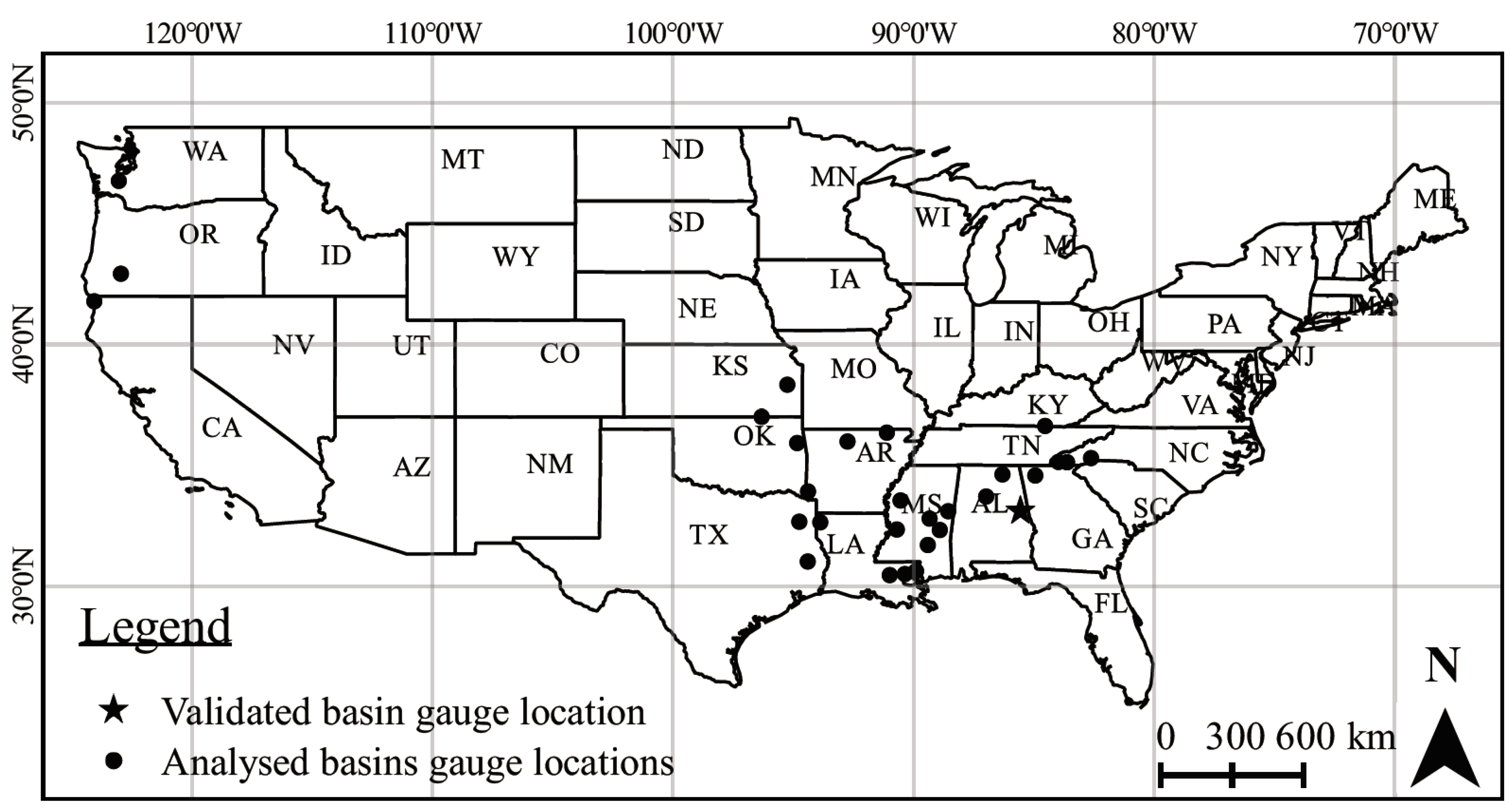
2.1. Study Area

This study analyzes 22 river basins across the USA. Stream gauge locations of the analyzed basins are shown in Figure 1. The river basins were selected based on prior calibration experience of the XAJ model by Rahman et al. [15]. Rahman et al. [15] selected these river basins to avoid snow impacts on SMM calculations and mentioned the XAJ model’s capability to simulate river discharge with good accuracies. This study selected the same river basins or basins located within the area analyzed by Rahman et al. [15] intending to reduce calibration efforts and to enable linking between SMM and spin-up time. Moreover, snow processes would introduce additional system memory and affect its spin-up behavior. Analyzed basins are located in nearly snow-free areas. Based on 30-year climate normals (1981–2010) released by NOAA’s National Climatic Data Centre [23], the basins have less than 7 snow-days (a snow-day is a day that records at least 2.5 mm snow/day) and receive less than 200 mm of total new snow per year. A summary of the analyzed basins’ physical and hydro-climatic characteristics is presented in Table 1.

Figure 1. Stream gauge location map over the USA mainland.

Figure 1. Stream gauge location map over the USA mainland.

2.2. Data

The basin scale daily precipitation, P (daily mean areal precipitation calculated from ground based gauge precipitation), potential evaporation, PE (developed from NOAA Evaporation Atlas), and streamflow, Q data (developed from USGS hydro-climatic data) were obtained from the U.S. Model Parameter Estimation Project (MOPEX) data sets [24,25].

Table 1. Studied MOPEX basins, locations and basic characteristics.

MOPEX ID	Location			Average Precipitation (mm/year)	Average Potential Evaporation (mm/year)	Average Snow-Days (day/year)	Average Total New Snow (mm/year)	Average Soil Moisture Saturation (%)
	Longitude	Latitude	State
11532500	−124.05	41.79	CA	2687	740	0.00	0	82
12027500	−123.03	46.78	WA	1599	579	3.00	127	75
03550000	−83.98	35.14	NC	1846	771	3.90	193	75
03504000	−83.62	35.13	NC	1893	762	3.90	193	90
03410500	−84.53	36.63	TN	1389	817	6.20	160	74
02387500	−84.94	34.58	GA	1480	901	0.70	18	73
03574500	−86.31	34.62	AL	1467	941	0.80	41	74
14308000	−122.95	42.93	OR	1347	805	2.20	76	62
07378500	−90.99	30.46	LA-MS	1594	1077	0.60	23	63
07375500	−90.36	30.51	LA-MS	1633	1074	0.60	23	64
02492000	−89.90	30.63	LA-MS	1583	1071	0.60	23	47
02456500	−86.98	33.71	AL	1425	982	0.80	41	66
02414500 *	−85.56	33.12	AL	1370	975	0.80	41	65
02472000	−89.41	31.71	MS	1492	1060	0.60	23	64
02448000	−88.56	33.10	MS	1421	1057	0.60	23	72
07290000	−90.70	32.35	MS	1435	1073	0.60	23	57
07056000	−92.75	35.98	AR	1180	916	3.80	132	68
07288500	−90.54	33.55	MS	1381	1112	0.60	23	62
07340000	−94.39	33.92	OK	1329	1156	5.60	198	70
07072000	−91.11	36.35	AR	1114	964	3.80	132	62
07348000	−93.88	32.65	LA	1173	1223	0.10	0	47
07346050	−94.75	32.67	TX	1128	1246	1.3	4	53
06914000	−95.25	38.33	KS	957	1206	10.00	373	61

Notes: * Indicates the validated river basin in Alabama, USA; bold face, Italic font style indicates dry basins (ζ > 0.9).

Table 1. Studied MOPEX basins, locations and basic characteristics.

MOPEX ID	Location			Average Precipitation (mm/year)	Average Potential Evaporation (mm/year)	Average Snow-Days (day/year)	Average Total New Snow (mm/year)	Average Soil Moisture Saturation (%)
	Longitude	Latitude	State
11532500	−124.05	41.79	CA	2687	740	0.00	0	82
12027500	−123.03	46.78	WA	1599	579	3.00	127	75
03550000	−83.98	35.14	NC	1846	771	3.90	193	75
03504000	−83.62	35.13	NC	1893	762	3.90	193	90
03410500	−84.53	36.63	TN	1389	817	6.20	160	74
02387500	−84.94	34.58	GA	1480	901	0.70	18	73
03574500	−86.31	34.62	AL	1467	941	0.80	41	74
14308000	−122.95	42.93	OR	1347	805	2.20	76	62
07378500	−90.99	30.46	LA-MS	1594	1077	0.60	23	63
07375500	−90.36	30.51	LA-MS	1633	1074	0.60	23	64
02492000	−89.90	30.63	LA-MS	1583	1071	0.60	23	47
02456500	−86.98	33.71	AL	1425	982	0.80	41	66
02414500 *	−85.56	33.12	AL	1370	975	0.80	41	65
02472000	−89.41	31.71	MS	1492	1060	0.60	23	64
02448000	−88.56	33.10	MS	1421	1057	0.60	23	72
07290000	−90.70	32.35	MS	1435	1073	0.60	23	57
07056000	−92.75	35.98	AR	1180	916	3.80	132	68
07288500	−90.54	33.55	MS	1381	1112	0.60	23	62
07340000	−94.39	33.92	OK	1329	1156	5.60	198	70
07072000	−91.11	36.35	AR	1114	964	3.80	132	62
07348000	−93.88	32.65	LA	1173	1223	0.10	0	47
07346050	−94.75	32.67	TX	1128	1246	1.3	4	53
06914000	−95.25	38.33	KS	957	1206	10.00	373	61

Notes: * Indicates the validated river basin in Alabama, USA; bold face, Italic font style indicates dry basins (ζ > 0.9).

2.3. Xinanjiang Model Parameters, Calibration and Validation

The runoff formation in the XAJ model is based on the repletion of storage concept, where the runoff starts to generate once the soil moisture content of the unsaturated zone reaches its field capacity, and subsequently runoff equals the rainfall excess without further loss [19]. Inputs to the XAJ model are areal mean precipitation and potential evaporation. Input data sets throughout this manuscript indicate time series of daily precipitation and potential evaporation. Streamflow from the whole basin is the output. There are 15 parameters in the XAJ model [26] and those could be determined by basin characteristics [19]. A list of XAJ model parameters and their ranges is presented in Table 2.

Table 2. Parameters in the Xinanjiang model.

Parameter	Physical Meaning	Range
Cp	Ratio of measured precipitation to actual precipitation	0.8–1.2
Cep	Ratio of potential evaporation to pan evaporation	0–2.0
b	Exponent of the tension water capacity curve	0.1–0.3
imp	Ratio of the impervious to the total area of the basin	0–0.005
WUM	Water capacity in the upper soil layer (mm)	5–20
WLM	Water capacity in the lower soil layer (mm)	60–90
WDM	Water capacity in the deeper soil layer (mm)	10–100
C	Coefficient of deep evaporation	0.1–0.3
SM	Areal mean free water capacity of the surface soil layer (mm)	1–50
EX	Exponent of the free water capacity curve	0.5–2.5
KI	Outflow coefficient of the free water storage to interflow	0–0.7; KI + KG = 0.7
KG	Outflow coefficient of the free water storage to groundwater	0–0.7; KI + KG = 0.7
cs	Recession constant for channel routing	0.5–0.9
ci	Recession constant for the lower interflow storage	0.5–0.9
cg	Daily recession constant of groundwater storage	0.9835–0.998

Table 2. Parameters in the Xinanjiang model.

Parameter	Physical Meaning	Range
Cp	Ratio of measured precipitation to actual precipitation	0.8–1.2
Cep	Ratio of potential evaporation to pan evaporation	0–2.0
b	Exponent of the tension water capacity curve	0.1–0.3
imp	Ratio of the impervious to the total area of the basin	0–0.005
WUM	Water capacity in the upper soil layer (mm)	5–20
WLM	Water capacity in the lower soil layer (mm)	60–90
WDM	Water capacity in the deeper soil layer (mm)	10–100
C	Coefficient of deep evaporation	0.1–0.3
SM	Areal mean free water capacity of the surface soil layer (mm)	1–50
EX	Exponent of the free water capacity curve	0.5–2.5
KI	Outflow coefficient of the free water storage to interflow	0–0.7; KI + KG = 0.7
KG	Outflow coefficient of the free water storage to groundwater	0–0.7; KI + KG = 0.7
cs	Recession constant for channel routing	0.5–0.9
ci	Recession constant for the lower interflow storage	0.5–0.9
cg	Daily recession constant of groundwater storage	0.9835–0.998

The XAJ model calibration for this study has been carried out with the aid of a web-based application [27,28].

This web platform not only allows the user to calibrate the XAJ model in a user friendly environment, but also provides: firstly, helpful calibration support by suggesting parameter settings developed by Li and Lu [26]; and secondly, hydrograph visualization and calculating Nash-Sutcliffe (NASH) efficiency [29]. NASH efficiency was calculated based on Equation (1).

$$NASH=1-\frac{{\displaystyle {\sum }_{t=1}^n{\left[Q_o(t)-Q_s(t)\right]}^2}}{{\displaystyle {\sum }_{t=1}^n{\left[Q_o(t)-{\overline{Q}}_o\right]}^2}}$$

(1)

where Q_o, Q_s and ${\overline{Q}}_o$ are the observed daily streamflow, simulated daily streamflow, and average observed daily streamflow, respectively.

2.4. Recursive Simulation Design

To detect the spin-up trends, one-year input data from 1 January to 31 December was repeated in a yearly cycle for 10 years. A similar recursive experiment was done in several model spin-up studies [8,11,13,14]. This yearly recursive simulation removes inter-annual climate variability and links any model adjustment processes to the equilibrium state of its internal stores (i.e., soil moisture) from an initial anomaly directly to the spin-up processes. However, this single-year recursive simulation may not be able to represent an accurate climatology, and may or may not achieve an unnatural equilibrium [30]. To overcome this limitation, recursive simulations were done with three separate input data sets representing mean, 5th and 95th percentile climatology.

2.4.1. Preparation of Input Files

Streamflow for each basin was simulated with three separate input files, created with a single year data that is close to: (i) 5th percentile; (ii) mean; and (iii) 95th percentile climatology. To maintain consistency among the simulations, a single parameter set was used to simulate all three input files. However, practically, it is very unlikely to achieve good calibration accuracy for different climatologies using same parameter set due to the difference in water balance and high parameter sensitivity to precipitation (some basins would even produce negative NASH efficiency). As a solution, we tried to manipulate the input data sets in such a way that can represent different climatologies by keeping the same distribution pattern throughout the year. The input to the XAJ model is precipitation and potential evaporation. The potential evaporation climatology does not vary between a “dry year” and “wet year”. Therefore, we opted to generate hypothetical precipitation (also streamflow for validation purposes) climatology by manipulating that of the mean year. This modification aimed to gain relatively good calibration accuracy while still capturing the climatology. The objective of this study is to present the spin-up behavior under different climatologies. The modified intra-year precipitation distribution definitely differs from the actual one. However, we believe that this is still sufficient to fulfil our objective. This experimental design may not be the perfect one, but it is an improvement from earlier approaches.

Firstly, the mean, 5th percentile and 95th percentile precipitation and streamflow climatology were computed from 52-year observed data sets (1948–1999). Secondly, the year that closely represents the mean year climatology was selected to prepare the mean year input file by repeating 1 January to 31 December for 10 years. Thirdly, 5th percentile and 95th percentile input files were created by manipulating the mean year precipitation and streamflow data based on Equations (2) and (3).

$$P_{x,i}=P_{mean,i}\times \frac{P_x}{P_{mean}}$$

(2)

$$Q_{x,i}=Q_{mean,i}\times \frac{Q_x}{Q_{mean}}$$

(3)

where P_mean,i and P_x,i are the ith day precipitation for the mean and 5th or 95th percentile year, respectively; Q_mean,i and Q_x,i are the ith day streamflow for the mean and 5th or 95th percentile year, respectively; P_x, Q_x, P_mean and Q_mean are annual precipitation for the 5th or 95th percentile year, annual streamflow for the 5th or 95th percentile year, annual precipitation for the mean year and annual streamflow for the mean year, respectively.

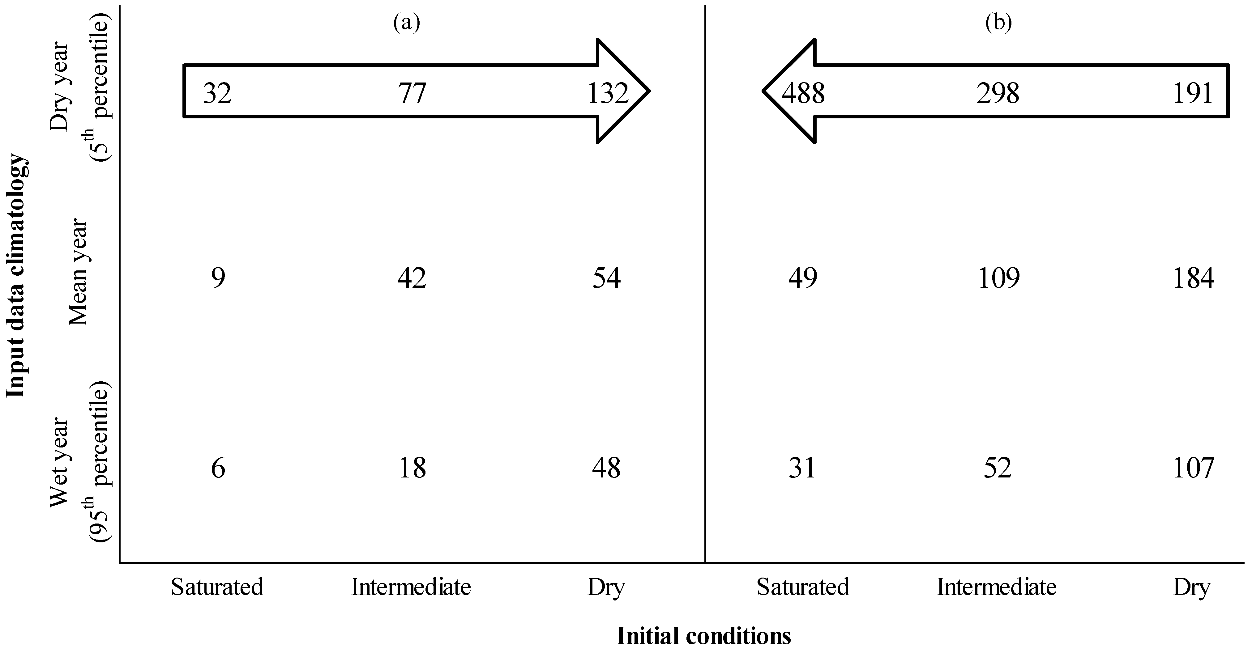
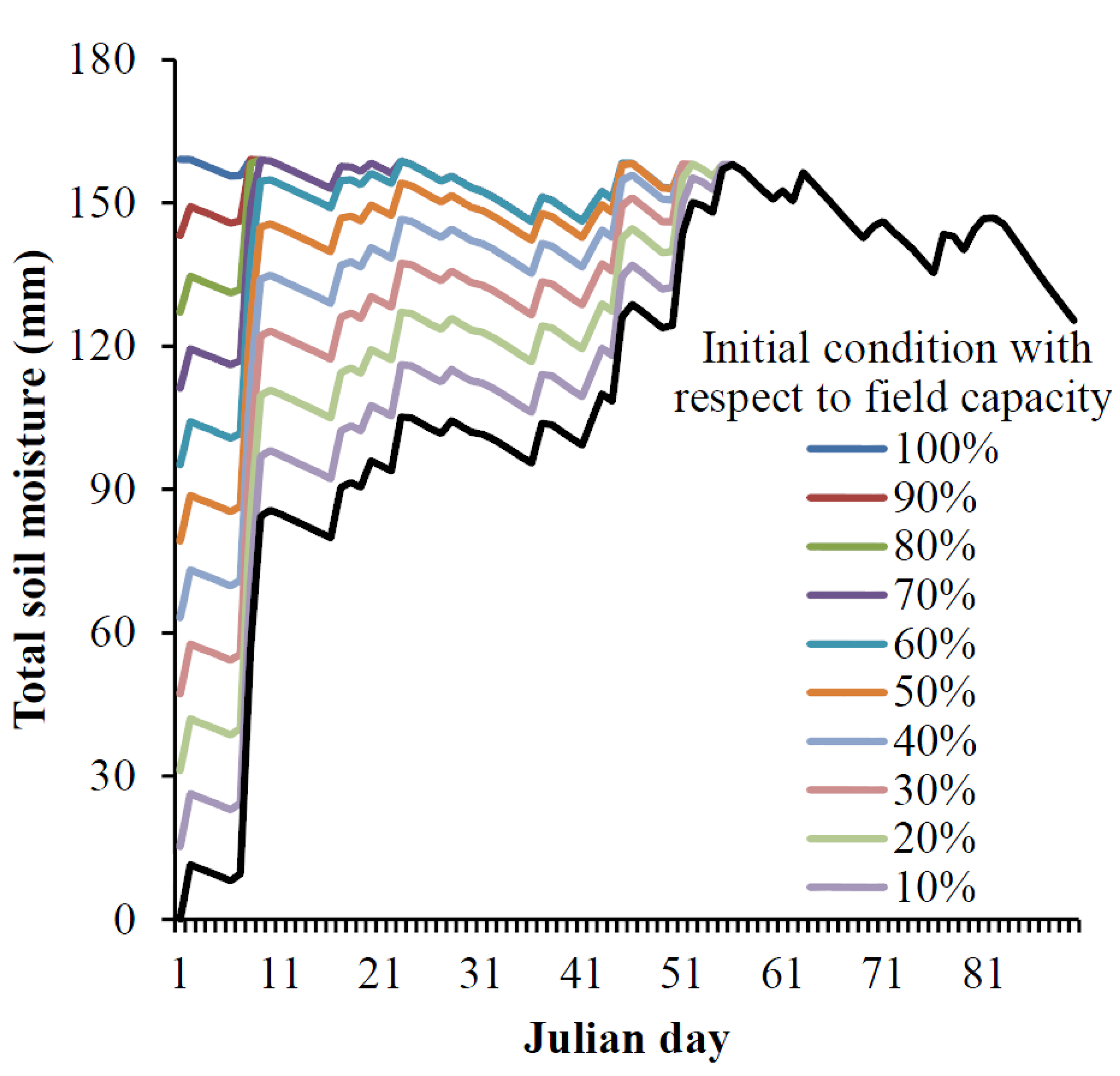
2.4.2. Initial Conditions

The XAJ model was run with four soil moisture initial conditions for each of the input climatology. The details of initial conditions are given in Table 3.

Table 3. Xinanjiang model soil moisture initial conditions.

Initial Condition	Physical Meaning
Saturated	100% of the field capacity
Intermediate	50% of the field capacity
Dry	Zero soil moisture
Climatology	Mean climatology initial condition

Table 3. Xinanjiang model soil moisture initial conditions.

Initial Condition	Physical Meaning
Saturated	100% of the field capacity
Intermediate	50% of the field capacity
Dry	Zero soil moisture
Climatology	Mean climatology initial condition

2.4.3. Model Calibration

The XAJ model was firstly calibrated with the mean year input file declaring an initial condition as intermediate. Once it achieves a good agreement between the daily observed and simulated discharge, the same parameter sets were used for the remaining simulations. A total of twelve simulations (4 initial conditions × 3 climatologies for each basin) were conducted for each basin. Average layered soil moisture values, obtained from the output of first simulation (mean year input file with an intermediate initial condition) were considered to be the average climatology of the basin.

2.5. Definition of Model Spin-Up Time

There are several accepted definitions of model equilibrium or spin-up. Yang et al. [8] define a complete model equilibrium state as the state at which the “model’s state at year n+1 is identical to that at year n”. However, in practice, it is very difficult to achieve identical sates between two recursive simulations, thus quite a few approaches have been proposed [11]. Spin-up can be defined based on the e-folding time (time required to reduce the yearly differences in daily/monthly model output to its 1/e value) [31], halving time (time required to reduce the yearly differences in daily/monthly model output to its half) [32] or percent cut off-based (PC) time (time required for yearly changes in daily/monthly model output to decrease to a certain threshold; see Cosgrove et al. [11] and de Goncalves et al. [9]). Of these, PC time has been widely used for detecting the model equilibrium [8,9,11,14,18,33,34].

In this study, the model equilibrium state has been defined on the basis of PC time. PC time defines the extent of time required for yearly changes in daily model output to decrease to a certain threshold. Generally, the threshold value for the model equilibrium varies from 1% to 0.01% depending on the purpose and scope [8,9,11,14,33]. This study detects the equilibrium at 0.01% threshold. The percentage change of daily values of total soil moisture was calculated by Equation (4).

$$PC=|\frac{D_{n,i}-D_{n+1,i}}{D_{n+1,i}}|\times 100$$

(4)

where PC, D_n,i and D_n+1,i are the percentage change, the total soil moisture at day i of year n and n+1, respectively.

2.6. Reporting of Model Spin-Up Time

Every basin produces twelve different spin-up times (4 initial conditions × 3 climatologies for each basin). The analysis relating to the basin aridity index considers the highest spin-up time produced by the initial condition that is closest to the average climatology. The average saturation of the river basins is shown in Table 1. The average saturation of 18 out of 22 river basins is close to 50% of their respective field capacities. Therefore, the spin-up time produced with an intermediate initial condition was reported for those basins. The remaining four river basins seem to have average saturation close to their full capacity, and thus spin-up times produced with a saturated initial condition was reported for those basins (first four basins of Table 1).

As discussed earlier, the model achieves an equilibrium state quickly under less SMM conditions. Rahman et al. [15] argued that soil moisture state loses all the memory once it becomes saturated. In harmony, this study also assumes that the XAJ model will take little or no time to achieve an equilibrium state under highly wet conditions (aridity index approaches zero). Thus, the regression equation presented in this paper, which shows the relationship between the spin-up time and aridity index, was optimized so that the model’s behavior in arid conditions beyond the examined basins could be better understood.

2.7. Calculation of Basin Aridity Index and Soil Moisture Memory

The aridity index value, ζ was calculated from independent sets of precipitation and potential evaporation data. The aridity index was estimated by interpolating the aridity index values of 400 MOPEX river basins across the USA (excluding the basins analyzed in this paper). The aridity index was calculated after Li and Lu [26], Equation (5).

$$\text{ζ}=\frac{PE}{P}$$

(5)

where ζ, PE and P are the aridity index, mean annual potential evaporation and ground-based mean annual areal precipitation, respectively.

The interpolation was done employing the Kriging method with the aid of the ArcGIS Spatial Analyst tool (version 10.0). The interpolated aridity index values showed high agreement with those of calculated (using the 53-years precipitation and potential evaporation data used for climatological analysis) ones with an r² values of 0.99. Consistent with Rahman et al. [15], the river basins are grouped as wet (ζ < 0.9) and dry (ζ > 0.9) basins for simplicity of analysis.

The basin average soil moisture memory (SMM) timescale in days was estimated after Rahman et al. [15] using Equation (6).

$${\text{τ}}_{SMM}=24.76(e^{1.25\text{ζ}}-1)$$

(6)

where τ_SMM is the SMM timescale in days and ζ is the basin aridity index.

3. Results and Discussion

3.1. Hydrograph, SMM Timescale and Aridity Index

The daily NASH efficiencies of the analyzed basins range from 0.43 to 0.87. The validated daily hydrograph for the mean year simulation is presented in Figure 2. The validation result suggests that the simulated daily streamflow agrees very well with those of daily observed streamflow. The basin-wise range of NASH efficiency, SMM timescale and aridity index are included in Table 4.

Figure 2. Validated daily hydrograph of 20 analyzed river basins (calibrated with mean year input data sets). MOPEX ID is presented in parenthesis.

Figure 2. Validated daily hydrograph of 20 analyzed river basins (calibrated with mean year input data sets). MOPEX ID is presented in parenthesis.

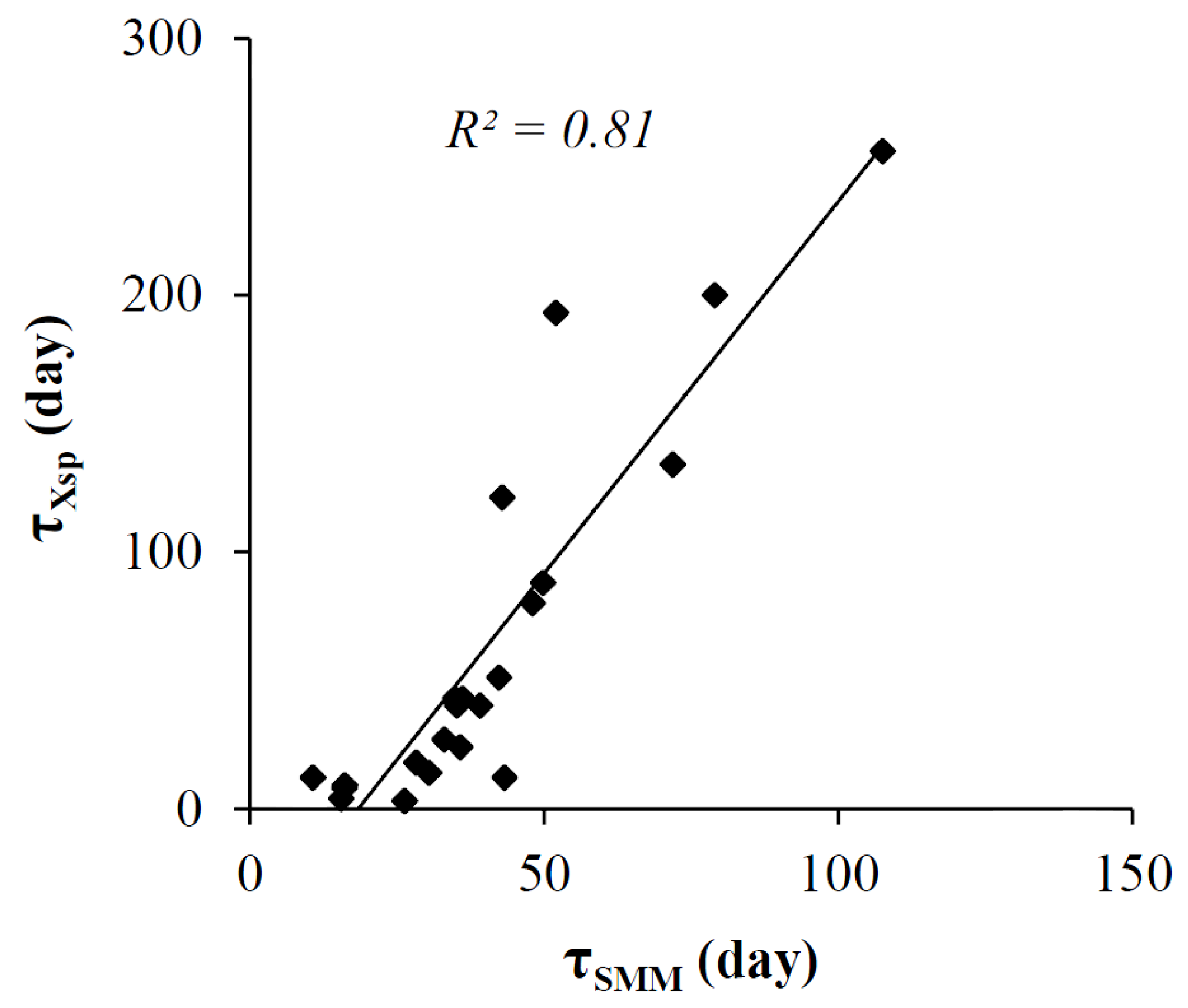
3.2. XAJ Model Spin-Up Time and SMM Timescale

Analyzed basins’ spin-up time ranged from 2 to 655 days. The wet basins (ζ < 0.9) require less time (mean spin-up time 55 days) to be equilibrated compared to the dry basins (ζ > 0.9; mean spin-up time 298 days). Basin-wise model spin-up times produced with an initial condition that is close to the average climatology (intermediate for 18 basins and saturated for 4 basins) are given in Table 4.

Table 4. Summary of the XAJ model spin-up time analysis.

MOPEX ID	Area (sq.km)	Daily NASH	Aridity Index (ζ)	τSMM (day)	τXsp (day)
11532500	1577	0.70–0.75	0.29	11	7
12027500	2318	0.71–0.73	0.39	16	3
03550000	269	0.58–0.72	0.40	16	2
03504000	135	0.70–0.77	0.40	16	9
03410500	2471	0.59–0.70	0.58	26	14
02387500	4144	0.67–0.72	0.61	28	18
03574500	829	0.72–0.82	0.64	30	23
14308000	1163	0.77–0.84	0.68	33	27
07378500	3315	0.43–0.61	0.70	35	43
07375500	1673	0.75–0.85	0.71	35	40
02492000	3142	0.77–0.82	0.71	36	24
02456500	2292	0.65–0.70	0.72	36	43
02414500 *	2696	0.79	0.73	37	55
02472000	1924	0.48–0.79	0.76	39	40
02448000	1989	0.43–0.83	0.80	42	73
07290000	7283	0.54–0.61	0.80	43	131
07056000	2147	0.64–0.81	0.81	43	65
07288500	1987	0.75–0.84	0.86	48	68
07340000	6895	0.58–0.61	0.88	50	342
07072000	1134	0.61–0.87	0.90	52	192
07348000	8125	0.46–0.71	1.09	72	134
07346050	383	0.55–0.74	1.15	79	211
06914000	865	0.43–0.69	1.34	108	655

Notes: * Indicates the validated river basin in Alabama, USA; bold face, Italic font style indicate dry basins (ζ > 0.9).

Table 4. Summary of the XAJ model spin-up time analysis.

MOPEX ID	Area (sq.km)	Daily NASH	Aridity Index (ζ)	τSMM (day)	τXsp (day)
11532500	1577	0.70–0.75	0.29	11	7
12027500	2318	0.71–0.73	0.39	16	3
03550000	269	0.58–0.72	0.40	16	2
03504000	135	0.70–0.77	0.40	16	9
03410500	2471	0.59–0.70	0.58	26	14
02387500	4144	0.67–0.72	0.61	28	18
03574500	829	0.72–0.82	0.64	30	23
14308000	1163	0.77–0.84	0.68	33	27
07378500	3315	0.43–0.61	0.70	35	43
07375500	1673	0.75–0.85	0.71	35	40
02492000	3142	0.77–0.82	0.71	36	24
02456500	2292	0.65–0.70	0.72	36	43
02414500 *	2696	0.79	0.73	37	55
02472000	1924	0.48–0.79	0.76	39	40
02448000	1989	0.43–0.83	0.80	42	73
07290000	7283	0.54–0.61	0.80	43	131
07056000	2147	0.64–0.81	0.81	43	65
07288500	1987	0.75–0.84	0.86	48	68
07340000	6895	0.58–0.61	0.88	50	342
07072000	1134	0.61–0.87	0.90	52	192
07348000	8125	0.46–0.71	1.09	72	134
07346050	383	0.55–0.74	1.15	79	211
06914000	865	0.43–0.69	1.34	108	655

Notes: * Indicates the validated river basin in Alabama, USA; bold face, Italic font style indicate dry basins (ζ > 0.9).

Average spin-up times of the XAJ model in wet and dry basins for all three input data sets with four initial conditions are shown in Figure 3. Spin-up time tends to increase with the dryness of initial conditions in all basins for both mean and 95th percentile input data sets. In contrast, wet and dry basins respond differently when the XAJ model is run with the 5th percentile input data sets. XAJ model spin-up time increases with dryness of the initial conditions for wet basins while calibrated with the 5th percentile input data sets. In contrast, the XAJ model takes less time to achieve equilibrium for the 5th percentile input data sets with dry initial condition. In wet basins, saturated initial condition requires less time to reach equilibrium. Similarly, Seck et al. [13] also suggests that spin-up for dry initial condition is slower than that of wet initial conditions. However, available literature does not clarify which initial condition should facilitate equilibrium condition in the least amount of time.

We believe that any initial condition that is close to the average climatology should theoretically lead to equilibrium quickly. In wet basins (average climatology around 70% of the field capacity), dry initial condition creates maximum anomalies, and, thus, would take the longest time to reach equilibrium. Similarly, in dry basins (average climatology slightly over 50% of the field capacity), dry initial conditions also create the maximum number of anomalies, and thus might equilibrate slowly. In both wet and dry basins, we expected that the intermediate initial condition (50% of the field capacity) would achieve equilibrium quickly. However, the present study reveals that the XAJ model consistently tends to achieve equilibrium quickly under saturated initial conditions for all the basins (except for dry basins simulated with 5th percentile input data sets) irrespective to their average climatology. This might be an XAJ model dependent phenomena and the XAJ model would always approach equilibrium quickly under a saturated initial condition. Moreover, the XAJ model seems to behave differently under dry-dry (dry basins simulation with dry climatologies) conditions. The exceptional behavior of the XAJ model spin-up time, while simulating with 5th percentile climatology, could be better understood by analyzing drier basins. Unfortunately, the XAJ model is reported to work better under humid and semi-humid conditions [19,20,26], thus, such investigation under dry-dry conditions would be challenging. Nevertheless, the outcomes of the present study would be essential for the application of the XAJ model for most of the areas.

Figure 3. Average XAJ model spin-up time (in days) produced with different initial conditions and input data sets; (a) wet basins (ζ < 0.9) (b) dry basins (ζ > 0.9).

Figure 3. Average XAJ model spin-up time (in days) produced with different initial conditions and input data sets; (a) wet basins (ζ < 0.9) (b) dry basins (ζ > 0.9).

Among the input data sets, the 95th percentile exhibits the least spin-up time requirement for any initial condition. Moreover, saturated initial condition with the 95th percentile input data sets displayed the minimum time requirement to be equilibrated. Figure 3 reveals that the XAJ model spin-up time tends to increase with both the dryness of initial condition and the climatology of input data sets. Therefore, the findings of the present study indicate that, for wet basins, a saturated initial condition could save XAJ model spin-up time, regardless of the input data set climatologies. However, for dry basins, a drier initial condition could be wise in the case where the input data sets represent a drier climatology.

Model simulation with climatology initial conditions also disclosed a substantial time requirement for the XAJ model equilibrium. This implies that model initialization, based on observed or model derived climatological mean, may not always be sufficient to avoid the spin-up error. A precise model initialization might also require spin-up time to be considered for subsequent analysis. Estimated model spin-up time (with climatology initial condition) exhibits a strong agreement with the basin average SMM timescales (calculated from independent data sets) with an r² of 0.81 (Figure 4). This is consistent with Cosgrove et al.’s [11] argument regarding the association between model equilibrium and soil moisture persistence.

Figure 4. Relationship between basin-wise soil moisture memory and XAJ model spin-up time.

Figure 4. Relationship between basin-wise soil moisture memory and XAJ model spin-up time.

This high r² value not only indicates the influence of soil moisture anomaly dissipation speed on the model spin-up time, but also justifies the use of recursive simulation to detect the XAJ model’s spin-up behavior. Even though a single year’s forcing data was used to run the model in a recursive way, it can still sufficiently capture the basin’s characteristics.

3.3. Predictability of XAJ Model Spin-Up Time from Basin Aridity Index

Literature [13,14] suggests that spin-up time for an integrated hydrological model is much longer than that which is typically reported for LSMs. Comparing spin-up time of models of different types would be a very difficult task. Soil moisture persistence is stronger compared with those of meteorological fluxes [35]. Similarly, soil moisture persistence in the deeper layer is much stronger than that of the surface layer [36,37,38]. Therefore, the model spin-up study considering equilibrium for different state variable (sensible/latent heat flux, total soil moisture, root zone soil moisture, depth of water table, discharge, ground water storage, etc.) would provide different results. However, model spin-up behavior (how it approaches equilibrium under different circumstances) could be compared quite easily. The XAJ model’s spin-up behavior seems to be consistent with those of LSMs. Noah’s LSM spin-up study [18] on the Korean Data Assimilation System argued that dry land areas take more than 40 months for spin-up, compared to wet areas. Similarly, Rodell et al. [12] claimed that Mosaic [39] LSM shows less spin-up time in humid regions compared to arid regions. Moreover, Cosgrove et al. [11] demonstrated a strong spatial variation and correlation of spin-up time with precipitation and temperature.

Computed basin-wise XAJ model spin-up time (mostly with an intermediate initial condition) reveals an exponential relationship with basin aridity index (calculated from independent data sets) with an r² value of 0.85 (Figure 5). The relationship between the basin aridity index and model spin-up time can be expressed by Equation (7).

$${\text{τ}}_{Xsp}=3.65\left(e^{3.83\text{ζ}}-1\right)$$

(7)

where τ_Xsp is the XAJ model spin-up time in days and ζ is the basin aridity index.

Figure 5. Relationship between basin aridity index and XAJ model spin-up time.

Figure 5. Relationship between basin aridity index and XAJ model spin-up time.

This relationship could be useful for roughly estimating the maximum XAJ model spin-up time when no information about the soil moisture climatology is available. This equation may not provide the exact spin-up duration, but could be useful for a safe estimation to avoid the spin-up error. Annual scale precipitation and potential evapotranspiration datasets are widely available compared that of soil moisture climatology, and thus would aid modeling exercises under data scarce situations. Declaring an intermediate initial condition is easy and straightforward compared to setting a climatology initial condition. However, it should be noted that this relationship is based on the daily scale model simulation only, thus, the XAJ model spin-up times for shorter or longer scales might be different.

The equation was validated against the actual spin-up behavior of the XAJ model for the Tallapoosa River Basin, Alabama, USA (MOPEX ID # 02414500; ζ = 0.73, gauge location shown in Figure 1). The equation suggests a maximum spin-up time of 56 days for a basin with an aridity index of 0.73. A recursive simulation with several initial conditions (mean year input data) indicates that the model takes a maximum of 55 days to reach an equilibrium soil moisture state (dry initial condition, see Figure 6). Theoretically, a spin-up time produced with the climatologic initial condition would be even closer to the physical state. However, considering the difficulty in setting a climatology initial condition, this study prefers to report the relationship based on the spin-up time produced with an intermediate initial condition.

Figure 6. Time series plot of total column soil moisture (mm) over the 11 year simulation for validated river basin at Alabama, USA (the Tallapoosa River basin, MOPEX ID # 02414500).

Figure 6. Time series plot of total column soil moisture (mm) over the 11 year simulation for validated river basin at Alabama, USA (the Tallapoosa River basin, MOPEX ID # 02414500).

4. Conclusions

Spin-up is the process during which a model adjusts its internal stores to an equilibrium state from an unusual initial state. Model outputs during this adjustment process are highly affected by the initial conditions, and consequently could be unrealistic and misleading. To avoid this problem, modelers often prefer to set the model initial condition as close to the reality and/or exclude the model outputs for the first few months. However, studies suggest that perfect initialization may not be sufficient for eliminating the risk of erroneous model output. The model adjustment process is not only affected by the initial condition but also by the characteristics of input data sets. Similarly, exclusion of the first few months’ model outputs is not an ideal solution. Exclusion of model output, guided by a feeling, could lead to underestimating or overestimating spin-up time. Therefore, prior information about the model’s behavior under different conditions or preferable initial conditions will improve the detection of spin-up time or reducing spin-up time, respectively. This study investigates the XAJ model’s spin-up behavior using different initial conditions and input data sets (representing separate climatology) for 22 river basins across the USA.

The XAJ model shows an increasing trend of spin-up times against both the dryness in input data sets and initial conditions. The responses are identical in wet and dry basins for the mean and 95th percentile input data sets. In contrast, it behaves differently in wet and dry basins for the 5th percentile input data sets. In wet basins, spin-up times tend to increase with the dryness of initial conditions, while dryer initial conditions produces less spin-up time in dry basins. Among the input data sets, 95th percentile exhibited the least spin-up time requirement, regardless of the basin dryness. For all the basins, a 95th percentile input data sets with saturated initial condition showed the minimum time to be equilibrated. Analysis suggests that a saturated initial condition is preferable for a mean year or 95th percentile data sets for all the basins. However, it would be wise to utilize saturated and dry initial condition for the dryer input data sets (5th percentile) for wet and dry basins, respectively.

Finally, the wet basins require less time for model equilibrium compared to those of dry basins. The spin-up time displays a high correlation with the basin soil moisture memory timescale. Moreover, the XAJ model spin-up timescale exhibits an exponential relationship with basin aridity index. This relationship allows estimation of the XAJ model spin-up time using only precipitation and evaporation information. Estimation of the XAJ model spin-up time could be valuable to reduce uncertainty associated with the guessing of spin-up time, based simply on feeling or experience. Prior information about model spin-up time would allow us to fully use the information included in short data records under data scarce situations.

References

1. Berthet, L.; Andréassian, V.; Perrin, C.; Javelle, P. How crucial is it to account for the antecedent moisture conditions in flood forecasting? Comparison of event-based and continuous approaches on 178 catchments. Hydrol. Earth Syst. Sci. 2009, 13, 819–831. [Google Scholar] [CrossRef]
2. Castillo, V.; Gomez-Plaza, A.; Martinez-Mena, M. The role of antecedent soil water content in the runoff response of semiarid catchments: A simulation approach. J. Hydrol. 2003, 284, 114–130. [Google Scholar] [CrossRef]
3. Goodrich, D.; Schmugge, T.; Jackson, T.; Unkrich, C.; Keefer, T.; Parry, R.; Bach, L.; Amer, S. Runoff simulation sensitivity to remotely sensed initial soil water content. Water Resour. Res. 1994, 30, 1393–1405. [Google Scholar] [CrossRef]
4. Minet, J.; Laloy, E.; Lambot, S.; Vanclooster, M. Effect of high-resolution spatial soil moisture variability on simulated runoff response using a distributed hydrologic model. Hydrol. Earth Syst. Sci. 2011, 15, 1323–1338. [Google Scholar] [CrossRef]
5. Nikolopoulos, E.I.; Anagnostou, E.N.; Borga, M.; Vivoni, E.R.; Papadopoulos, A. Sensitivity of a mountain basin flash flood to initial wetness condition and rainfall variability. J. Hydrol. 2011, 402, 165–178. [Google Scholar] [CrossRef]
6. Senarath, S.U.; Ogden, F.L.; Downer, C.W.; Sharif, H.O. On the calibration and verification of two-dimensional, distributed, Hortonian, continuous watershed models. Water Resour. Res. 2000, 36, 1495–1510. [Google Scholar] [CrossRef]
7. Zhang, Y.; Wei, H.; Nearing, M. Effects of antecedent soil moisture on runoff modeling in small semiarid watersheds of southeastern Arizona. Hydrol. Earth Syst. Sci. 2011, 15, 3171–3179. [Google Scholar] [CrossRef]
8. Yang, Z.L.; Dickinson, R.; Henderson-Sellers, A.; Pitman, A. Preliminary study of spin-up processes in land surface models with the first stage data of Project for Intercomparison of Land Surface Parameterization Schemes Phase 1 (a). J. Geophys. Res. Atmos. 1995, 100, 16553–16578. [Google Scholar] [CrossRef]
9. De Goncalves, L.; Shuttleworth, W.J.; Burke, E.J.; Houser, P.; Toll, D.L.; Rodell, M.; Arsenault, K. Toward a South America Land Data Assimilation System: Aspects of land surface model spin-up using the Simplified Simple Biosphere. J. Geophys. Res. Atmos. 2006, 111. [Google Scholar] [CrossRef]
10. Chen, F.; Mitchell, K. Using the GEWEX/ISLSCP forcing data to simulate global soil moisture fields and hydrological cycle for 1987–1988. J. Meteorol. Soc. Japan 1999, 77, 167–182. [Google Scholar]
11. Cosgrove, B.A.; Lohmann, D.; Mitchell, K.E.; Houser, P.R.; Wood, E.F.; Schaake, J.C.; Robock, A.; Sheffield, J.; Duan, Q.; Luo, L.; et al. Land surface model spin-up behaviour in the North American Land Data Assimilation System (NLDAS). J. Geophys. Res. Atmos. 2003, 108. [Google Scholar] [CrossRef]
12. Rodell, M.; Houser, P.; Berg, A.; Famiglietti, J. Evaluation of 10 methods for initializing a land surface model. J. Hydrometeorol. 2005, 6, 146–155. [Google Scholar] [CrossRef]
13. Seck, A.; Welty, C.; Maxwell, R.M. Spin-up behavior and effects of initial conditions for an integrated hydrologic model. Water Resour. Res. 2015, 15. [Google Scholar] [CrossRef]
14. Ajami, H.; McCabe, M.F.; Evans, J.P.; Stisen, S. Assessing the impact of model spin-up on surface water-groundwater interactions using an integrated hydrologic model. Water Resour. Res. 2014, 50, 2636–2656. [Google Scholar] [CrossRef]
15. Rahman, M.M.; Lu, M.; Kyi, K.H. Variability of soil moisture memory for wet and dry basins. J. Hydrol. 2015, 523, 107–118. [Google Scholar] [CrossRef]
16. Ajami, H.; Evans, J.; McCabe, M.; Stisen, S. Technical Note: Reducing the spin-up time of integrated surface water-groundwater models. Hydrol. Earth Syst. Sci. Discuss. 2014, 18, 5169–5179. [Google Scholar] [CrossRef]
17. Wood, E.F.; Lettenmaier, D.P.; Liang, X.; Lohmann, D.; Boone, A.; Chang, S.; Chen, F.; Dai, Y.; Dickinson, R.E.; Duan, Q.; et al. The project for Intercomparison of Land-surface Parameterization Schemes (PILPS) phase 2 (c) Red-Arkansas River basin experiment: 1. Experiment description and summary intercomparisons. Glob. Planet. Chang. 1998, 19, 115–135. [Google Scholar] [CrossRef]
18. Lim, Y.J.; Hong, J.; Lee, T.Y. Spin-up behaviour of soil moisture content over East Asia in a land surface model. Meteorol. Atmos. Phys. 2012, 118, 151–161. [Google Scholar] [CrossRef]
19. Zhao, R.J. The Xinanjiang model applied in China. J. Hydrol. 1992, 135, 371–381. [Google Scholar]
20. Lu, M.; Li, X. Time scale dependent sensitivities of the Xinanjiang model parameters. Hydrol. Res. Lett. 2014, 8, 51–56. [Google Scholar] [CrossRef]
21. Lin, C.A.; Wen, L.; Lu, G.; Wu, Z.; Zhang, J.; Yang, Y.; Zhu, Y.; Tong, L. Atmospheric-hydrological modeling of severe precipitation and floods in the Huaihe River Basin, China. J. Hydrol. 2006, 330, 249–259. [Google Scholar] [CrossRef]
22. Lu, G.; Wu, Z.; Wen, L.; Lin, C.A.; Zhang, J.; Yang, Y. Real-time flood forecast and flood alert map over the Huaihe River Basin in China using a coupled hydro-meteorological modeling system. Sci. China Ser. E Technol. Sci. 2008, 51, 1049–1063. [Google Scholar] [CrossRef]
23. National Climate Data Center. Available online: http://www.ncdc.noaa.gov/oa/climate/normals/usnormals.html (accessed on 13 November 2013).
24. Schaake, J.; Cong, S.; Duan, Q. The US MOPEX Data Set. Publication number 307; International Association of Hydrological Sciences Publication: Oxfordshire, UK, 2006. [Google Scholar]
25. Model Parameter Estimation Experiment. Available online: ftp://hydrology.nws.noaa.gov/pub/gcip/mopex/US_Data/ (accessed on 19 October 2013).
26. Li, X.; Lu, M. Application of aridity index in estimation of data adjustment parameters in the Xinanjiang model. Annu. J. Hydraul. Eng. JSCE 2014, 58, 163–168. [Google Scholar] [CrossRef]
27. Kyi, K.H. Development of a User Friendly Web-Based Xinanjiang Model with Calibration Support System. Master Thesis, Department of Civil and Environmental Engineering, Nagaoka University of Technology, Nagaoka, Japan, 2014. [Google Scholar]
28. Laboratory of Hydrology and Meteorology. Available online: http://lmj.nagaokaut.ac.jp/~khin/ (accessed on 13 January 2015).
29. Nash, J.E.; Sutcliffe, J.V. River flow forecasting through conceptual models part-I: A discussion of principles. J. Hydrol. 1970, 10, 282–290. [Google Scholar] [CrossRef]
30. Schlosser, C.A.; Slater, A.G.; Robock, A.; Pitman, A.J.; Vinnikov, K.Y.; Henderson-Sellers, A.; Speranskaya, N.A.; Mitchell, K. Simulations of a boreal grassland hydrology at Valdai, Russia: PILPS Phase 2 (d). Mon. Weather Rev. 2000, 128, 301–321. [Google Scholar] [CrossRef]
31. Delworth, T.L.; Manabe, S. The influence of potential evaporations on the variabilities of simulated soil wetness and climate. J. Clim. 1988, 1, 523–547. [Google Scholar] [CrossRef]
32. Simmonds, I.; Lynch, A.H. The influence of pre-existing soil moisture content on Australian winter climate. Int. J. Clim. 1992, 12, 33–54. [Google Scholar] [CrossRef]
33. Henderson-Sellers, A.; McGuffie, K.; Pitman, A. The project for inter-comparison of land-surface parametrization schemes (PILPS): 1992 to 1995. Clim. Dyn. 1996, 12, 849–859. [Google Scholar] [CrossRef]
34. Chen, T.H.; Henderson-Sellers, A.; Milly, P.; Pitman, A.; Beljaars, A.; Polcher, J.; Abramopoulos, F.; Boone, A.; Chang, S.; Chen, F.; et al. Cabauw experimental results from the project for inter-comparison of land-surface parameterization schemes. J. Clim. 1997, 10, 1194–1215. [Google Scholar] [CrossRef]
35. Koster, R.D.; Suarez, M.J. Soil moisture memory in climate models. J. Hydrometeorol. 2001, 2, 558–570. [Google Scholar] [CrossRef]
36. Vinnikov, K.Y.; Robock, A.; Speranskaya, N.A.; Schlosser, C.A. Scales of temporal and spatial variability of midlatitude soil moisture. J. Geophys. Res. Atmos. 1996, 101, 7163–7174. [Google Scholar] [CrossRef]
37. Entin, J.K.; Robock, A.; Vinnikov, K.Y.; Hollinger, S.E.; Liu, S.; Namkhai, A. Temporal and spatial scales of observed soil moisture variations in the extratropics. J. Geophys. Res. Atmos. 2000, 105, 11865–11877. [Google Scholar] [CrossRef]
38. Wu, W.; Dickinson, R.E. Time Scales of Layered Soil Moisture Memory in the Context of Land-Atmosphere Interaction. J. Clim. 2004, 17, 2752–2764. [Google Scholar] [CrossRef]
39. Koster, R.D.; Suarez, M.J. Modeling the land surface boundary in climate models as a composite of independent vegetation stands. J. Geophys. Res. Atmos. 1992, 97, 2697–2715. [Google Scholar] [CrossRef]