Spatio-Temporal Variations and Source Apportionment of Water Pollution in Danjiangkou Reservoir Basin, Central China

Abstract

Understanding the spatio-temporal variation and the potential source of water pollution could greatly improve our knowledge of human impacts on the environment. In this work, data of 11 water quality indices were collected during 2012–2014 at 10 monitoring sites in the mainstream and major tributaries of the Danjiangkou Reservoir Basin, Central China. The fuzzy comprehensive assessment (FCA), the cluster analysis (CA) and the discriminant analysis (DA) were used to assess the water pollution status and analyze its spatio-temporal variation. Ten sites were classified by the high pollution (HP) region and the low pollution (LP) region, while 12 months were divided into the wet season and the dry season. It was found that the HP region was mainly in the small tributaries with small drainage areas and low average annual discharges, and it was also found that most of these rivers went through urban areas with industrial and domestic sewages input into the water body. Principal component analysis/factor analysis (PCA/FA) was applied to reveal potential pollution sources, whereas absolute principal component score-multiple linear regression (APCS-MLR) was used to identify their contributions to each water quality variable. The study area was found as being generally affected by industrial and domestic sewage. Furthermore, the HP region was polluted by chemical industries, and the LP region was influenced by agricultural and livestock sewage.

1. Introduction

More and more attention has been paid to surface water quality, as it is strongly relevant to human lives and public health [1,2]. However, as surface water quality is controlled by both natural factors (hydrological and meteorological conditions) and human influences (urban, industrial and agricultural activities), decision makers are facing with significant difficulties the problem of how to manage surface water quality [3,4,5]. Although water quality monitoring has greatly improved over the last few decades, a representative and reliable estimation of surface water quality is still challenging [6]. Therefore, the study of spatio-temporal variations and source apportionment of water pollution is especially essential in ecological environment protection and water resources management [7,8].

Datasets of water quality are usually complex containing huge amounts of information with internal relationships among variables, which make it difficult to interpret and draw meaningful conclusions [9]. Thus, in recent years, there has been an increasing interest by researchers in analyzing such complex data using robust mathematics and statistical techniques, such as fuzzy comprehensive evaluation method (FCA), cluster analysis (CA), discriminant analysis (DA), and principal component analysis/factor analysis (PCA/FA), and absolute principal component score–multiple linear regression (APCS-MLR) [10,11,12,13,14,15,16,17,18,19,20,21,22,23,24,25,26,27,28]. A literature review of these methods is described below.

FCA has been successfully applied to evaluate the pollution level of water quality since the 1990s [10]. For example, Lu et al. [11] developed a general methodology for fuzzy synthetic evaluation and studied the feasibility of the method by a case study of trophic status assessment for Fei-Tsui Reservoir in Taiwan. The result showed that the method could observe the long-term change of water quality and overturn phenomena, which would provide valuable information to decision makers and assist reservoir management. Similarly, Liou et al. [10] proposed a fuzzy index model for environmental quality evaluation, and proved that the model was flexible and adaptable for evaluating the eutrophic status of reservoir waters. A study conducted by Dahiya et al. [12] used FCA to assess the physico-chemical quality of groundwater for drinking purposes. The acceptability of the drinking water was determined based on the limit of different quality classes prescribed by regulatory bodies and the perception of the experts in the field. The results showed that 4, 23 and 15 samples were in “desirable,” “acceptable,” and “not acceptable” categories, respectively. Additionally, Huang et al. [13] applied the method to estimate water quality levels and group the monitoring sites in Qiantang River. The assessment criterion set of five levels in the study were derived based on national quality standards for surface waters in China. The river was classified into three major pollution zones (low, moderate, and high).

The primary purpose of CA is to classify samples into clusters with similar characteristics in water environment research. A study conducted by Varol [14] grouped the 10 sampling sites into three clusters with similar characteristic features and natural background using the CA technology in the Tigris River basin, Turkey. In a similar way, Yang et al. [15] used the method to detect temporal-spatial similarity and group the monitoring sites and periods in the Lake Dianchi watershed. A full 12 months were grouped into two periods: August–September and the remaining months, and the entire water area were divided into two clusters: site 1 and sites 2–8. The method can help to better understand spatial patterns and temporal variations of water quality by comparing among different groups, and to formulate an optimal sampling strategy on the basis of grouping information. For example, Gridharan et al. [16] applied CA to group stations in the River Cooum, South India, and suggested that the upper part of the river was classified into an unpolluted cluster, while the middle and lower parts of the river were grouped into a polluted cluster. Kazi et al. [9] grouped the monitoring sites in Manchar Lake (Pakistan) into three significant clusters—(sites 1 and 2), (site 4) and (sites 3 and 5) using the method, and suggested that only one station in each cluster was needed to represent a reasonably accurate spatial pattern of the water quality for the whole area. Hence, the number of sampling sites in the monitoring program would be reduced without losing any significant information.

DA was commonly performed on the data set to confirm the clusters determined by means of CA based on the accuracy rate of discriminant functions. For example, Papaioannou et al. [17] used the method to construct the discriminant functions on two different modes, i.e., standard and stepwise. The discriminant functions of the two different modes yielded a classification matrix correctly assigning 96.97% and 96.36% of the cases, respectively, which proved the reasonability of the classification. Besides, many studies have applied DA to bring out the most significant variables that result in water quality spatial and temporal variation, and to optimize the monitoring program by decreasing the number of parameters monitored. For example, Mustapha et al. [6] studied surface water quality variation using the DA method at the upper course of Kano River, Nigeria and suggested that seven variables were successfully separated among the 23 variables as the most statistically significant variables that brought spatial variation. A study conducted by Singh et al. [18] showed that DA offers an important data reduction by using only six variables discriminating spatial pattern and two variables for temporal variation in Gomti River, India. Similarly, Zhang et al. [19] applied the method to evaluate spatial-temporal variation of water quality in southwest new territories and Kowloon, Hong Kong, and revealed that four and eight parameters could afford 84.2% and 96.1% correct assignation in temporal and spatial analysis, respectively. Furthermore, they also suggested that the number of monitoring variables and the associated cost can be reduced, as the method afforded a considerable data reduction in the dimensionality of the large data set.

PCA/FA is a dimension-reduction technique that provides information by the most significant factors with a simpler representation of the data. Therefore, it has been utilized by various researchers to explore the pollution sources of a water environment system. For example, the method was employed by Lim et al. [20] to identify latent factors or pollution sources in Langat River, Malaysia. Four components were extracted with a total variance of 85% in group 1, while six components were extracted with a total variance of 88% in group 2. Based on this information, they discovered that sea water intrusion, agricultural and industrial pollution, and geological weathering were responsible for the river pollution for both groups. In addition, Tanriverdi et al. [21] applied PCA/FA to analyze and assess the surface water quality of Ceyhan River and suggested that the stations near cities were strongly affected by household wastewater, while the other stations were influenced by agricultural facilities. Moreover, Jha et al. [22] identified major pollution sources influencing the physico-chemical variables in Aerial Bay using the FA technique, which included rivulet influx into the bay, land run-off, prevailing biological processes and tidal flow.

PCA/FA can just provide qualitative information about pollution sources, but cannot provide quantitative contributions of each source type to each variable [23]. However, a receptor-based model, such as APCS-MLR can solve the problem [18]. The method was firstly used for pollution source identification and apportionment in an atmospheric environment [24]. In recent years, there have been many researchers using this method to apportion the pollution sources in water environment research, as it is less dependent on the number of sources or their compositions. For example, Singh et al. [18] applied APCS-MLR for source apportionment in three different catchment regions of the Gomti River and analyzed the quantitative contributions of various pollution sources to different water quality variables (e.g., the contributions of municipal and industrial water, and soil runoff to BOD is 98.0% and 2.0%, respectively, in upper catchment). Furthermore, this method was also used by Yang et al. [25] to quantitatively analyze the contribution of each pollution source in Wen-Rui-Tang (WRT) river watershed in China, and they suggested that 88.4% of NH₄⁺-N came from domestic sewage pollution and commercial/service pollution in the urban zone. Su et al. [26] studied the apportionment problem of pollution source for water quality in Qiantang River, China with this method (e.g., the effect of chemical pollution to COD_Mn is 73.2%).

These studies provided invaluable insights into the applications of FCA, CA, DA, PCA/FA, and APCS-MLR methods in environmental research and how these methods can handle large datasets of water quality with a large number of parameters, which enable the accurate attainment of the multivariate features of the water environment system [27]. The combined use of these methods can help to make full use of the advantages of each method and get a comprehensive understanding of the spatio-temporal variations and potential sources of water pollution.

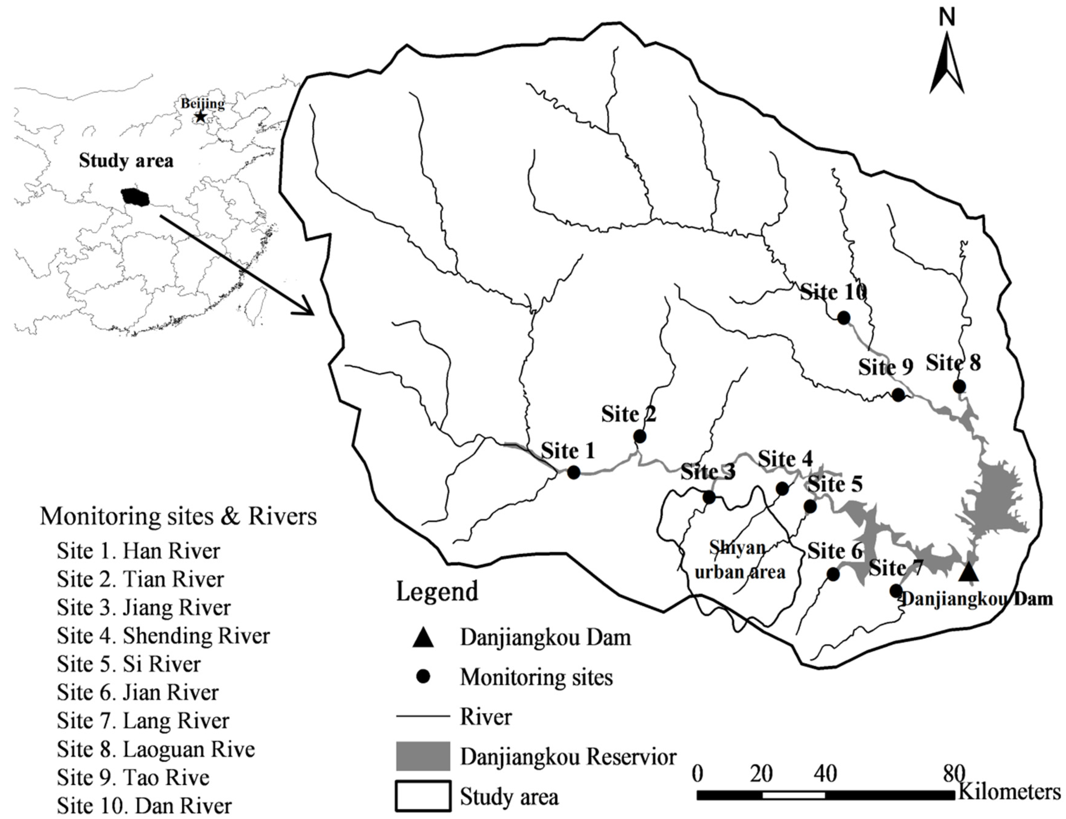
Many papers have been published that investigate the spatial and temporal variations of surface water quality in reservoirs or lakes [1,9,11,15,28]. However, these studies have mainly focused on water quality variations within the reservoirs or lakes, and attentions have rarely been paid to the water pollution of the rivers that flow into the reservoirs or lakes. In this study, water quality variations in the mainstream and major tributaries of the Danjiangkou Reservoir Basin were studied based on FCA, CA, DA, PCA/FA, and APCS-MLR methods. The objectives of this study are (1) to analyze temporal and spatial variations of water quality in the study area; (2) to identify potential pollution sources; and (3) to estimate the contributions of the potential pollution sources to each water quality variable.

2. Materials and Methods

2.1. Study Area

Danjiangkou Reservoir Basin (32°36′ N~33°48′ N; 110°59′ E~111°49′ E, Figure 1) is located in the upper reaches of the Han River in central China, including Danjiangkou Reservoir and its upstream areas. It encompassed a drainage area of 9.52 × 10⁴ km². The study area is affected by a north sub-tropical monsoon climate with rapid and severe climate transitions. Annual mean temperature is 15–16 °C. Precipitation is subjected to large inter-annual variability, with 800–1000 mm∙year⁻¹, of which 80% is concentrated between May and September [29,30]. Danjiangkou Reservoir has an annual water supply capacity of 2.91 × 10¹⁰ m³, a surface area of 1022.75 km², and an annual average runoff of 3.79 × 10¹⁰ m³. It is one of the main water sources of the South-to-North Water Transfer Project in China, and responsible for the water supply of Beijing, Tianjin and more than 130 other cities in northern China. Therefore, the water quality level is especially important to drinking water safety for these cities, and directly affects the feasibility of the water transfer project.

Figure 1. Study area and monitoring sites.

Figure 1. Study area and monitoring sites.

2.2. Water Samples

Water samples were collected in monthly intervals between April 2012 and March 2014 at ten monitoring sites in the mainstream and major tributaries of Danjiangkou Reservoir Basin (Figure 1). Eleven water quality indexes were selected for analysis, including water temperature (Temp), pH, dissolved oxygen (DO), chemical O₂ demand (COD_Mn), 5-day biochemical oxygen demand (BOD₅), total phosphorus (TP), ammonium nitrogen (NH₄⁺-N), fluorine (F⁻), arsenic (As), volatile phenol (V-ArOH), and fecal coliform (F. coli). These variables represent physical properties, aggregate organic constituents, nutrient constituents, or biological properties of the river. The sampling, preservation, transportation and analysis of the water samples were performed according to the environmental quality standard for surface water of China (GB3838-2002). The specific analytical method used is shown in Table 1. The univariate statistics of the water quality parameters are presented in Table 2.

Table 1. Water quality parameters, units and analytical methods used during 2012–2014 for the Danjiangkou Reservoir Basin.

Parameter	Unit	Analytical method
Temp	°C	Thermometer
pH	--	Glass electrode
DO	mg·L−1	Iodometric
CODMn	mg·L−1	Potassium permanganate method
BOD5	mg·L−1	Dilution and inoculation test
TP	mg·L−1	Ammonium molybdate spectrophotometry
NH4+-N	mg·L−1	N-reagent colorimetry
F−	mg·L−1	Ion chromatography
As	mg·L−1	Silver diethyldithiocarbamate spectrophotography
V-ArOH	mg·L−1	Spectrophotometric Determination with 4-Amino-Antipyrin
F. coli	num·L−1	Multi-tube zymolytic methodMembrane filter method

Table 1. Water quality parameters, units and analytical methods used during 2012–2014 for the Danjiangkou Reservoir Basin.

Parameter	Unit	Analytical method
Temp	°C	Thermometer
pH	--	Glass electrode
DO	mg·L−1	Iodometric
CODMn	mg·L−1	Potassium permanganate method
BOD5	mg·L−1	Dilution and inoculation test
TP	mg·L−1	Ammonium molybdate spectrophotometry
NH4+-N	mg·L−1	N-reagent colorimetry
F−	mg·L−1	Ion chromatography
As	mg·L−1	Silver diethyldithiocarbamate spectrophotography
V-ArOH	mg·L−1	Spectrophotometric Determination with 4-Amino-Antipyrin
F. coli	num·L−1	Multi-tube zymolytic methodMembrane filter method

Table 2. Univariate statistics of the water quality parameters.

Parameters		Site 1	Site 2	Site 3	Site 4	Site 5	Site 6	Site 7	Site 8	Site 9	Site 10
N		24	24	24	24	24	24	24	24	24	24
Temp (°C)	Mean	17.55	17.43	18.87	20.04	17.83	17.82	19.08	17.61	17.90	16.72
	SD	6.38	6.75	7.72	6.27	7.60	7.91	8.62	8.71	7.95	8.12
pH	Mean	8.12	7.89	7.73	7.54	7.60	7.91	8.30	7.88	8.10	8.10
	SD	0.20	0.19	0.26	0.13	0.20	0.44	0.49	0.13	0.14	0.16
DO (mg∙L−1)	Mean	9.77	8.72	8.24	3.96	5.02	8.84	12.03	7.93	10.72	9.82
	SD	1.68	3.27	2.79	2.97	2.20	3.68	3.71	3.36	1.84	1.85
CODMn (mg∙L−1)	Mean	1.79	1.58	5.58	8.95	6.01	5.28	3.28	2.85	1.44	1.84
	SD	0.59	0.81	2.19	3.61	1.14	1.87	0.87	0.92	0.45	1.20
BOD5 (mg∙L−1)	Mean	0.85	1.36	3.98	14.59	5.05	3.25	2.00	1.97	1.02	0.92
	SD	0.29	1.08	2.15	17.23	2.95	1.60	1.13	1.63	0.44	0.37
TP (mg∙L−1)	Mean	0.04	0.05	0.81	0.80	0.65	0.12	0.17	0.09	0.02	0.07
	SD	0.03	0.03	0.86	0.50	0.27	0.09	0.16	0.05	0.01	0.05
NH4+-N (mg∙L−1)	Mean	0.08	0.14	2.10	8.99	5.46	1.93	0.21	0.82	0.07	0.39
	SD	0.08	0.19	2.09	2.82	1.90	3.01	0.24	0.90	0.04	0.43
F− (mg∙L−1)	Mean	0.16	0.21	0.31	0.60	0.40	0.24	0.16	0.25	0.20	0.28
	SD	0.04	0.04	0.08	0.17	0.08	0.05	0.06	0.05	0.04	0.05
As (mg∙L−1)	Mean	0.001	0.002	0.003	0.002	0.002	0.002	0.002	0.002	0.002	0.002
	SD	0.000	0.001	0.001	0.001	0.001	0.000	0.001	0.001	0.001	0.001
V-ArOH (mg∙L−1)	Mean	0.001	0.001	0.002	0.003	0.002	0.001	0.001	0.001	0.001	0.001
	SD	0.001	0.000	0.002	0.004	0.004	0.001	0.001	0.000	0.001	0.001
F. coli (num L−1)	Mean	3702	7935	434,917	873,542	175,892	14,829	3463	10,445	1071	1421
	SD	2049	4193	604,229	914,210	332,154	36,347	5918	17,918	1758	3215

Note: N number of samples, SD standard deviation.

Table 2. Univariate statistics of the water quality parameters.

Parameters		Site 1	Site 2	Site 3	Site 4	Site 5	Site 6	Site 7	Site 8	Site 9	Site 10
N		24	24	24	24	24	24	24	24	24	24
Temp (°C)	Mean	17.55	17.43	18.87	20.04	17.83	17.82	19.08	17.61	17.90	16.72
	SD	6.38	6.75	7.72	6.27	7.60	7.91	8.62	8.71	7.95	8.12
pH	Mean	8.12	7.89	7.73	7.54	7.60	7.91	8.30	7.88	8.10	8.10
	SD	0.20	0.19	0.26	0.13	0.20	0.44	0.49	0.13	0.14	0.16
DO (mg∙L−1)	Mean	9.77	8.72	8.24	3.96	5.02	8.84	12.03	7.93	10.72	9.82
	SD	1.68	3.27	2.79	2.97	2.20	3.68	3.71	3.36	1.84	1.85
CODMn (mg∙L−1)	Mean	1.79	1.58	5.58	8.95	6.01	5.28	3.28	2.85	1.44	1.84
	SD	0.59	0.81	2.19	3.61	1.14	1.87	0.87	0.92	0.45	1.20
BOD5 (mg∙L−1)	Mean	0.85	1.36	3.98	14.59	5.05	3.25	2.00	1.97	1.02	0.92
	SD	0.29	1.08	2.15	17.23	2.95	1.60	1.13	1.63	0.44	0.37
TP (mg∙L−1)	Mean	0.04	0.05	0.81	0.80	0.65	0.12	0.17	0.09	0.02	0.07
	SD	0.03	0.03	0.86	0.50	0.27	0.09	0.16	0.05	0.01	0.05
NH4+-N (mg∙L−1)	Mean	0.08	0.14	2.10	8.99	5.46	1.93	0.21	0.82	0.07	0.39
	SD	0.08	0.19	2.09	2.82	1.90	3.01	0.24	0.90	0.04	0.43
F− (mg∙L−1)	Mean	0.16	0.21	0.31	0.60	0.40	0.24	0.16	0.25	0.20	0.28
	SD	0.04	0.04	0.08	0.17	0.08	0.05	0.06	0.05	0.04	0.05
As (mg∙L−1)	Mean	0.001	0.002	0.003	0.002	0.002	0.002	0.002	0.002	0.002	0.002
	SD	0.000	0.001	0.001	0.001	0.001	0.000	0.001	0.001	0.001	0.001
V-ArOH (mg∙L−1)	Mean	0.001	0.001	0.002	0.003	0.002	0.001	0.001	0.001	0.001	0.001
	SD	0.001	0.000	0.002	0.004	0.004	0.001	0.001	0.000	0.001	0.001
F. coli (num L−1)	Mean	3702	7935	434,917	873,542	175,892	14,829	3463	10,445	1071	1421
	SD	2049	4193	604,229	914,210	332,154	36,347	5918	17,918	1758	3215

Note: N number of samples, SD standard deviation.

2.3. Statistical Analysis and Data Treatments

FCA is a process of evaluating water quality utilizing the fuzzy set theory. It assesses the significance of multiple pollutants according to weights and decreases the fuzziness by using membership functions [10]. The mathematical details of the FCA method can be found in the relevant literature [13]. The assessment criteria of five water quality grades were established according to the GB3838-2002 standard in the study (Table 3).

Table 3. Environmental guideline of national quality standards for surface water, China (GB3838-2002).

Parameter	Units	I	II	III	IV	V
DO ≥	mg·L−1	7.5	6	5	3	2
CODMn ≤	mg·L−1	2	4	6	10	15
BOD5 ≤	mg·L−1	3	3	4	6	10
TP ≤	mg·L−1	0.02	0.1	0.2	0.3	0.4
NH4+-N ≤	mg·L−1	0.15	0.5	1	1.5	2
F− ≤	mg·L−1	1	1	1	1.5	1.5
As ≤	mg·L−1	0.05	0.05	0.05	0.1	0.1
V-ArOH ≤	mg·L−1	0.002	0.002	0.005	0.01	0.1
F. coli ≤	num·L−1	200	2000	10,000	20,000	40,000

Table 3. Environmental guideline of national quality standards for surface water, China (GB3838-2002).

Parameter	Units	I	II	III	IV	V
DO ≥	mg·L−1	7.5	6	5	3	2
CODMn ≤	mg·L−1	2	4	6	10	15
BOD5 ≤	mg·L−1	3	3	4	6	10
TP ≤	mg·L−1	0.02	0.1	0.2	0.3	0.4
NH4+-N ≤	mg·L−1	0.15	0.5	1	1.5	2
F− ≤	mg·L−1	1	1	1	1.5	1.5
As ≤	mg·L−1	0.05	0.05	0.05	0.1	0.1
V-ArOH ≤	mg·L−1	0.002	0.002	0.005	0.01	0.1
F. coli ≤	num·L−1	200	2000	10,000	20,000	40,000

Multivariate analysis of the water quality was performed using four techniques: CA, DA, PCA/FA and APCS–MLR. CA is an unsupervised pattern detection method with the primary purpose of assembling objects to different clusters based on the characteristics they possesses [31]. The most common approach of CA is hierarchical clustering (HCA), which can provide similarity relationships between any one sample and whole data set [7]. In this study, HCA was performed on the standardized dataset by the Ward’s method, and squared Euclidean distances were used as a measure of similarity. DA is a method to conform the groups found by CA and determines the most significant water quality variables. In this analysis, three different modes of DA, i.e., standard, forward stepwise and backward stepwise, were applied to evaluate both the spatial and temporal variations in water quality [32]. PCA is a powerful pattern recognition method, making use of a small set of independent variables to describe the variance of a relatively large dataset [33]. FA further reduces the contribution of these less significant variables through VARIMAX rotation, and produces new groups of variation called variance factors (VFs). VFs can include unobservable, hypothetical and latent variables [34]. The VFs are explained based on the factor loadings, which were classified as “strong,” “moderate,” and “weak,” corresponding to absolute loading values of >0.75, 0.75–0.50 and 0.50–0.30 [35]. To quantify the contribution of each pollution source to each measured variable, the APCS-MLR method is often used. The computation of APCS-MLR for each sample is followed by the regression of sample mass concentrations on these APCS to derive each identified source’s estimated mass contribution [36].

Most multivariate statistical techniques require the variables to be normally distributed [37], but the original data showed that most of the variables were far from normal with 95% confidence examined by the skewness and kurtosis statistical tests. Therefore, the original data were logarithmic transformed [38]. The skewness and kurtosis values for the log-transformed data were significantly reduced and consistent to the normal distribution. All log-transformed variables were further z-scale standardized for CA, PCA/FA and APCS-MLR, whereas original data was used for DA. The CA and DA were made using STATISTICA 7.0, PCA/FA and APCS-MLR used SPSS 13.0, and FCA used Microsoft Excel 2010.

3. Results and Discussion

3.1. Water Quality Evaluation

The water quality for all sampling sites and monitoring months was evaluated using FCA based on the GB3838-2002 standard; the results are shown in Table 4. According to the standard, water quality of class I and II was regarded as low pollution status, while water quality of class III, IV and V was regarded as high pollution status. Among the 10 sampling sites, water quality in site 1, site 2, site 9 and site 10 (Han River, Tian River, Tao river and Dan River) was very good (class I), while it was much worse (class V) in site 3, site 4 site 5 and site 6 (Jiang River, Shending River, Si River and Jian River) for almost the whole year. The water quality in site 7 and site 8 (Lang River and Laoguan River) was less satisfactory from April to August.

Table 4. Results of water quality assessment.

Time	Site 1	Site 2	Site 3	Site 4	Site 5	Site 6	Site 7	Site 8	Site 9	Site10
January	I	I	V	V	V	III	I	I	I	I
February	I	III	V	V	V	V	I	I	I	I
March	I	I	V	V	V	V	I	I	I	I
April	I	I	V	V	V	V	III	III	I	I
May	I	I	V	V	V	V	II	II	I	I
June	I	I	V	V	V	V	II	III	I	I
July	I	I	V	V	V	V	III	V	I	I
August	I	I	V	V	V	V	III	II	I	I
September	I	I	V	V	V	III	III	I	I	I
October	I	I	V	V	V	III	I	I	I	I
November	I	I	V	V	V	II	I	I	I	I
December	I	I	IV	V	V	I	I	I	I	I

Table 4. Results of water quality assessment.

Time	Site 1	Site 2	Site 3	Site 4	Site 5	Site 6	Site 7	Site 8	Site 9	Site10
January	I	I	V	V	V	III	I	I	I	I
February	I	III	V	V	V	V	I	I	I	I
March	I	I	V	V	V	V	I	I	I	I
April	I	I	V	V	V	V	III	III	I	I
May	I	I	V	V	V	V	II	II	I	I
June	I	I	V	V	V	V	II	III	I	I
July	I	I	V	V	V	V	III	V	I	I
August	I	I	V	V	V	V	III	II	I	I
September	I	I	V	V	V	III	III	I	I	I
October	I	I	V	V	V	III	I	I	I	I
November	I	I	V	V	V	II	I	I	I	I
December	I	I	IV	V	V	I	I	I	I	I

3.2. Spatio-Temporal Similarity and Grouping

Spatial CA classified the 10 sampling sites into two groups at (Dlink/Dmax) × 100 < 60 (Figure 2a). Group A was comprised of site 3 to site 6 (Jiang River, Shending River, Si River, and Jian River), and group B consisted of the remaining sites. Based on the results of water quality assessment by FCA, group A could be considered as high pollution (HP), and group B could be considered as moderate or low pollution (LP). Using temporal CA, the 12 months were also classified into two clusters at (Dlink/Dmax) × 100 < 60 (Figure 2b). Cluster 1 contained May to October, closely corresponding to the wet season, and cluster 2 included the remaining months, corresponding to the dry season. The CA technique was useful in offering liable classification of surface water quality in the view of space and time. The sites in the same groups had similar natural backgrounds and features that may be affected by similar pollution sources. Therefore, the CA technique could reduce the need for numerous sampling stations and frequency, and could be used to design future spatio-temporal sampling strategies in an optimal manner [39].

Figure 2. Dendrograms showing (a) spatial clustering of sampling sites and (b) temporal clustering of monitoring periods.

Figure 2. Dendrograms showing (a) spatial clustering of sampling sites and (b) temporal clustering of monitoring periods.

In the study, the LP sites were located mainly in the main river channel (Han River) and the large tributaries (Tian River, Lang River, Laoguan River, Tao River and Dan River), whereas HP sites were in small tributaries (Jiang River, Shending River, Si River and Jian River). The drainage areas of the mainstream and large tributaries are all larger than 500 km² and the mean annual discharges of them are all larger than 3.5 m³·s⁻¹. Given the greater volume of flow in the mainstream, the river system has greater capacity to mitigate pollution loads than in the small tributaries [13]. Besides, most of the rivers in the HP region, such as Jiang River, Shending River and Si River, all went through the urban area of Shiyan City with more industrial effluent and domestic sewage entering the water body (Figure 1). Therefore, spatial distribution of water quality was determined by both natural factors and human activities. Similar distribution patterns were also found in other studies. For example, Gridharan et al. [16] found that in the River Cooum (South India), the upper part of the river was classified as an unpolluted cluster, while the middle and lower parts of the river were grouped into a polluted cluster, where settlements along the river course were dense and domestic wastewater was directly discharged into the water body. Varol [14] found that in the Tigris River basin (Turkey), low-concentration sites were close to the dam reflecting the natural background levels, whereas the high-concentration sites were located at the entrance of the streams to the reservoirs due to the human influence.

Previous results suggested that temporal variations of the water quality in Danjiangkou Reservoir Basin were greatly influenced by hydrological and meteorological conditions (wet season and dry season) in the area. However, 12 months could not be strictly divided into spring (March to May), summer (June to August), autumn (September to November) and winter (December to February), which indicated that temporal clustering of water quality did not present natural seasonal characteristic and hence it might be also affected by other reasons. One of the possible factors may be that effluent discharges of industrial wastewater and domestic wastewater discharge generally kept a relatively steady level throughout the year.

3.3. Spatial-Temporal Variations in Water Quality

To study the spatial variations of water quality, DA was applied on the raw data after dividing the whole data set into two groups (HP and LP). Discriminant functions (DFs) and classification matrixes (CMs) were shown in Table 5 and Table 6. The accuracy of spatial classification using standard, forward stepwise, and backward stepwise mode were 91.3% (11 discriminant variables), 90.8% (6 discriminant variables), and 90.8% (5 discriminant variables), respectively. The results indicated that pH, COD_Mn, BOD₅, NH₄⁺-N, and F⁻ were the most significant parameters for discrimination between the two groups and accounted for most of the expected spatial variations in water quality. For temporal DA, both the standard and forward stepwise mode, using 11 and 4 discriminant variables, respectively, yielded the corresponding CMs assigning 95.8% of the cases correctly. However, in backward stepwise mode, DA produced a CM with 95.4% correct assignation using only 3 discriminant parameters. Thus, the temporal DA results suggested that Temp, DO, and COD_Mn were the most significant parameters for discriminating differences between the wet season and dry season, and could be used to explain most of the expected temporal variations in water quality.

Table 5. Classification functions’ coefficients for discriminant analysis of spatial and temporal variations.

Parameters	Standard Mode		Forward Stepwise Mode		Backward Stepwise Mode
Spatial groups	HP	LP	HP	LP	HP	LP
Temp	−0.99	−0.96
pH	144.89	148.34	105.79	109.08	104.25	107.41
DO	−6.71	−6.74
CODMn	−1.69	−3.10	−0.81	−2.22	0.13	−1.19
BOD5	−0.28	−0.07	−0.16	0.05	−0.35	−0.15
TP	10.33	10.42
NH4+-N	3.86	3.64	5.71	5.48	5.38	5.13
F−	14.48	17.32	18.20	20.77	23.75	26.79
As	2873.55	3225.07	5038.76	5463.33
V-ArOH	−344.09	−387.76
F. coli	−0.01	−0.01
Constant	−537.01	−559.56	−425.12	−446.42	−416.86	−436.70
Temporal clusters	Wet season	Dry season	Wet season	Dry season	Wet season	Dry season
Temp	−0.96	−0.07	0.67	1.55	0.76	1.61
pH	145.66	145.34
DO	−6.76	−7.04	1.67	1.38	1.64	1.36
CODMn	0.93	0.49	1.28	0.77	1.31	0.8
BOD5	−0.76	−0.78
TP	13.49	13.54
NH4+-N	4.54	4.38
F−	2.88	5.11
As	3954.88	3200.47	1848.33	1262.71
V-ArOH	−367.72	−295.66
F. coli	−0.04	−0.03
Constant	−549.00	−557.85	−16.79	−27.35	−15.67	−26.82

Table 5. Classification functions’ coefficients for discriminant analysis of spatial and temporal variations.

Parameters	Standard Mode		Forward Stepwise Mode		Backward Stepwise Mode
Spatial groups	HP	LP	HP	LP	HP	LP
Temp	−0.99	−0.96
pH	144.89	148.34	105.79	109.08	104.25	107.41
DO	−6.71	−6.74
CODMn	−1.69	−3.10	−0.81	−2.22	0.13	−1.19
BOD5	−0.28	−0.07	−0.16	0.05	−0.35	−0.15
TP	10.33	10.42
NH4+-N	3.86	3.64	5.71	5.48	5.38	5.13
F−	14.48	17.32	18.20	20.77	23.75	26.79
As	2873.55	3225.07	5038.76	5463.33
V-ArOH	−344.09	−387.76
F. coli	−0.01	−0.01
Constant	−537.01	−559.56	−425.12	−446.42	−416.86	−436.70
Temporal clusters	Wet season	Dry season	Wet season	Dry season	Wet season	Dry season
Temp	−0.96	−0.07	0.67	1.55	0.76	1.61
pH	145.66	145.34
DO	−6.76	−7.04	1.67	1.38	1.64	1.36
CODMn	0.93	0.49	1.28	0.77	1.31	0.8
BOD5	−0.76	−0.78
TP	13.49	13.54
NH4+-N	4.54	4.38
F−	2.88	5.11
As	3954.88	3200.47	1848.33	1262.71
V-ArOH	−367.72	−295.66
F. coli	−0.04	−0.03
Constant	−549.00	−557.85	−16.79	−27.35	−15.67	−26.82

Table 6. Classification matrixes for discriminant analysis of spatial and temporal variations.

Monitoring Sites	Percent Correct, %	Spatial Groups		Monitoring Periods	Percent Correct, %	Temporal Clusters
		HP	LP			Wet Season	Dry Season
Standard mode
HP	81.25	78	18	Wet season	95.00	114	6
LP	97.92	3	141	Dry season	96.67	4	116
Total	91.25	81	159	Total	95.83	118	122
Forward stepwise mode
HP	80.21	77	19	Wet season	94.17	113	7
LP	97.92	3	141	Dry season	97.50	3	117
Total	90.83	80	160	Total	95.83	116	124
Backward stepwise mode
HP	80.21	77	19	Wet season	94.17	113	7
LP	97.92	3	141	Dry season	96.67	4	116
Total	90.83	80	160	Total	95.42	117	123

Table 6. Classification matrixes for discriminant analysis of spatial and temporal variations.

Monitoring Sites	Percent Correct, %	Spatial Groups		Monitoring Periods	Percent Correct, %	Temporal Clusters
		HP	LP			Wet Season	Dry Season
Standard mode
HP	81.25	78	18	Wet season	95.00	114	6
LP	97.92	3	141	Dry season	96.67	4	116
Total	91.25	81	159	Total	95.83	118	122
Forward stepwise mode
HP	80.21	77	19	Wet season	94.17	113	7
LP	97.92	3	141	Dry season	97.50	3	117
Total	90.83	80	160	Total	95.83	116	124
Backward stepwise mode
HP	80.21	77	19	Wet season	94.17	113	7
LP	97.92	3	141	Dry season	96.67	4	116
Total	90.83	80	160	Total	95.42	117	123

Box and whisker plots of the discriminant parameters were constructed to evaluate different patterns associated with spatial and temporal variations in water quality (Figure 3 and Figure 4). For spatial variations, the average pH value was slightly lower in the HP region, indicating that hydrolysis of the acidic material caused a decrease in pH value [31]. The natural background levels of pH values in these streams were greater than 7, owing to a Ca²⁺ and HCO₃⁻ type of water which was related with limestone soil in the study area [30]. Besides, the HP region had higher average concentrations of COD_Mn and BOD₅, which indicated that there was much more serious organic pollution. Furthermore, higher average value of NH₄⁺-N was found in the HP region, which suggested that the eutrophication might be a serious water quality problem in the region. Finally, average concentration of F⁻ was also higher in the HP region, indicating that the background values of fluoride were higher in the region, and groundwater inflow accounted for a significant proportion of river flow for these small tributaries. In summary, those spatial differences of the variables suggested that environment pollution problems in the HP region were worse than in the LP region and hence more attention should be paid to this region. For temporal variations, which are greatly affected by climatic conditions, the average temperature was higher in the wet season and lower in the dry. Furthermore, a clear inverse relationship between temperature and dissolved oxygen was observed. This could be explained that as water temperature increases in the river, biological activity of aquatic organism strengthens and therefore consumption of dissolved oxygen concentration increases. In addition, more oxygen also dissolves in cooler water. The average concentration of COD_Mn was slightly lower in the wet season than in the dry season, which was related to a greater volume of flow in the wet period.

Figure 3. Spatial variations: (a) pH; (b) COD_Mn; (c) BOD₅; (d) NH₄⁺-N; and (e) F⁻ in Danjiangkou Reservoir Basin.

Figure 3. Spatial variations: (a) pH; (b) COD_Mn; (c) BOD₅; (d) NH₄⁺-N; and (e) F⁻ in Danjiangkou Reservoir Basin.

Figure 4. Temporal variations: (a) Temp; (b) DO, and (c) COD_Mn in Danjiangkou Reservoir Basin.

Figure 4. Temporal variations: (a) Temp; (b) DO, and (c) COD_Mn in Danjiangkou Reservoir Basin.

3.4. Source Identification

In order to identify the potential pollution sources, PCA/FA was applied to the normalized log-transformed data sets for the two regions. Three variance factors (VFs) were obtained for the HP region and four VFs for the LP region with eigenvalues greater than 1, summing almost 67.0% and 71.2% of the total variance in the data set, respectively (Table 7).

Table 7. Loadings of 11 water quality variables on significant variance factors (VFs) for the high pollution (HP) and low pollution (LP) regions in Danjiangkou Reservoir Basin.

Parameters	HP			LP
	VF1	VF2	VF3	VF1	VF2	VF3	VF4
Temp	0.16	0.40	−0.79	0.00	−0.16	0.81	−0.24
pH	−0.57	−0.09	−0.39	0.08	0.85	0.09	−0.11
DO	−0.70	−0.23	0.19	0.06	0.78	−0.34	−0.11
CODMn	0.77	0.19	0.08	0.84	−0.09	0.26	−0.01
BOD5	0.80	−0.18	0.12	0.80	0.06	−0.22	−0.09
TP	0.73	0.46	0.26	0.80	−0.01	0.02	0.27
NH4+-N	0.81	0.16	0.31	0.49	−0.33	−0.20	0.52
F−	0.20	0.15	0.80	−0.04	0.01	−0.15	0.88
As	−0.04	0.86	0.00	0.31	−0.06	0.55	0.48
V-ArOH	0.33	0.65	−0.08	−0.06	−0.10	0.75	0.02
F. coli	0.74	0.11	−0.18	0.30	−0.73	0.22	−0.15
Eigenvalue	3.96	1.72	1.68	2.43	2.02	1.84	1.53
Total variance /%	36.03	15.64	15.29	22.13	18.39	16.73	13.95
Cumulative variance /%	36.03	51.67	66.96	22.13	40.52	57.25	71.20

Note: Bold and italic values indicate strong and moderate loadings, respectively.

Table 7. Loadings of 11 water quality variables on significant variance factors (VFs) for the high pollution (HP) and low pollution (LP) regions in Danjiangkou Reservoir Basin.

Parameters	HP			LP
	VF1	VF2	VF3	VF1	VF2	VF3	VF4
Temp	0.16	0.40	−0.79	0.00	−0.16	0.81	−0.24
pH	−0.57	−0.09	−0.39	0.08	0.85	0.09	−0.11
DO	−0.70	−0.23	0.19	0.06	0.78	−0.34	−0.11
CODMn	0.77	0.19	0.08	0.84	−0.09	0.26	−0.01
BOD5	0.80	−0.18	0.12	0.80	0.06	−0.22	−0.09
TP	0.73	0.46	0.26	0.80	−0.01	0.02	0.27
NH4+-N	0.81	0.16	0.31	0.49	−0.33	−0.20	0.52
F−	0.20	0.15	0.80	−0.04	0.01	−0.15	0.88
As	−0.04	0.86	0.00	0.31	−0.06	0.55	0.48
V-ArOH	0.33	0.65	−0.08	−0.06	−0.10	0.75	0.02
F. coli	0.74	0.11	−0.18	0.30	−0.73	0.22	−0.15
Eigenvalue	3.96	1.72	1.68	2.43	2.02	1.84	1.53
Total variance /%	36.03	15.64	15.29	22.13	18.39	16.73	13.95
Cumulative variance /%	36.03	51.67	66.96	22.13	40.52	57.25	71.20

Note: Bold and italic values indicate strong and moderate loadings, respectively.

In the HP region, the first variance factor (VF1) accounted for 36.0% of the total variance, had strong positive loadings on COD_Mn, BOD₅, and NH₄⁺-N, moderate negative loadings on pH and DO, and moderate positive loadings on TP and F. coli. Generally, COD_Mn is regarded as an organic pollution indicator from sources such as industrial wastewater and uncontrolled domestic sewage caused by rapid urbanization [18]. pH could regulate the concentrations of COD_Mn in the water, as it is one of the main reaction conditions in redox of organic matter [40,41]. High concentrations of nutrients (NH₄⁺-N, and TP) are usually from agricultural runoff, municipal effluents and fertilizer factory wastewater [15]. F. coli is mainly related to municipal wastes and animal husbandry [42]. Therefore, this factor could be interpreted as one typical kind of mixed pollution, which includes point source pollution, such as industrial effluent and domestic sewage, and non-point source pollution associated with agricultural activities [13]. VF1 could also represent an oxide-related process associated with negative DO and positive BOD₅. When organic matter in the river was oxidized at the expense of dissolved oxygen, the BOD₅ concentrations increased with decreasing DO [43]. VF2, accounting for 15.6% of the total variance, had strong positive loadings on As, and moderate positive loadings on V-ArOH. The element As is mainly from glass, paint, paper production and the coal combustion process [44]. V-ArOH is attributed to paper-making and chemical industries. This factor can be explained as chemical pollution, which resulted from industrial wastewater discharged into the river. Field work found that there were several paper mills in this region, e.g., the First Mill in Danjiangkou City and Yuyang Paper Mill in Yunxian County. However, some of them will be shut down or moved away due to water pollution problems. VF3 (15.3% of the total variance) had strong negative loadings on Temp and strong positive loadings on F⁻. F⁻ is usually from cement plants, fluorine chemical factories, and smelters [13]. However, in the region F⁻ levels at almost all monitoring sites were below 1.0 mg/L, which meant that there was almost no pollution. Such a small amount of fluoride may be influenced by local soils entering the river together with the runoff [13].

In the LP region, VF1, occupying about 22.1% of the total variance, had strong positive loadings on COD_Mn, BOD₅, and TP. This factor included organic pollution and nutrient pollution, and could be attributed to industrial effluent and domestic sewage. VF2 (18.4% of the total variance) had strong positive loadings on pH and DO. This factor represented physicochemical condition and biological state, and could be regarded as oxygen-consuming organic pollution [45]. Positive correction between pH and DO can be explained that as such: the amount of available DO decreases, an aerobic fermentation process happens, organic acids are produced, and then pH value decreases [42]. Moreover, the factor also had moderate negative loadings on F. coli, which may be caused by the effects of local livestock farm and domestic wastewater [45]. VF3, accounting for 16.7% of the total variance, had strong positive loadings on Temp and V-ArOH, moderate positive loadings on As. Concentration of As and V-ArOH at all monitoring sites were below 0.05 and 0.002 mg/L, respectively, basically representing natural factors. VF4 (14.0% of the total variance) had strong positive loadings on F⁻, and moderate positive loadings on NH₄⁺-N. In general, pollutions of NH₄⁺-N can be interpreted as nutrient pollution related to agricultural runoff and domestic wastewater [18]. Low concentrations of fluoride at all monitoring sites may also come from local soils entering the river, just like VF3 in the HP region.

Four types of pollution, including organic, nutrient, chemical and natural, were identified from the aspect of pollution composition in the previous analysis. Pollution sources could then be further identified based on this information. Firstly, organic pollution was mainly from point sources such as industrial effluent, domestic sewage and wastewater of local livestock farm. Secondly, nutrient pollution was generally from non-point source related with agricultural activities and point sources such as municipal effluents and fertilizer plant wastewater. Thirdly, chemical pollution was from wastewater of chemical industries. Finally, natural pollution was influenced by the changes of meteorological conditions such as the variation of water temperature. Two regions (HP and LP) were both mainly affected by industrial effluent and domestic sewage. In addition, a chemical pollution factor was also extracted from the HP region; independent oxygen-consuming organic pollution factor and nutrient pollution (N) factor were found in the LP region. This suggested that the HP region was also subjected to the influence of chemical industrial activities, while the LP region was also affected by livestock farming and agriculture activities. The identified pollution sources were different from those in other studies. For example, water quality in Langat River (Malaysia) was mainly influenced by the intrusion of saltine water, agricultural and industrial pollution, and geological weathering [20]. Major pollution sources in Aerial Bay consisted of rivulet flux, surface run-off, prevailing biological processes and tidal flow [22]. It was found that the type of source was mainly determined by the selected variables of water quality. Therefore, to better represent the pollution characteristics, the variables to be analyzed should be chosen appropriately.

To analyze the temporal variations of potential pollution sources, PCA/FA was also applied on the data set of each period for the two regions (Table 8). The results showed that temporal difference was significant in the HP region, which was associated with the smaller volume of flow in these rivers. A nutrient pollution factor, related with non-point pollution from agricultural activities, was distinguished from the mixed pollution in wet season. As crops grow mainly in this period, this phenomenon is partly because more nutrient pollutions were discharged into the river due to agricultural irrigation. However, in the LP region, the temporal difference of pollution sources was much smaller. As industrial and domestic pollution was relatively small, agricultural non-point source pollution could be distinguished in both periods.

Table 8. Results of source identification at wet season and dry season in high pollution (HP) region and low pollution (LP) region.

Periods	VF1	VF2	VF3	VF4	VF5
HP
Wet season	nutrient pollution	organic pollution	natural pollution	chemical pollution
Dry season	nutrient pollution + organic pollution	chemical pollution	natural pollution
LP
Wet season	organic pollution + nutrient pollution (P)	organic pollution (O)	natural pollution	nutrient pollution (N)	natural pollution
Dry season	organic pollution+ nutrient pollution (P)	organic pollution (O)	nutrient pollution (N)	natural pollution

Table 8. Results of source identification at wet season and dry season in high pollution (HP) region and low pollution (LP) region.

Periods	VF1	VF2	VF3	VF4	VF5
HP
Wet season	nutrient pollution	organic pollution	natural pollution	chemical pollution
Dry season	nutrient pollution + organic pollution	chemical pollution	natural pollution
LP
Wet season	organic pollution + nutrient pollution (P)	organic pollution (O)	natural pollution	nutrient pollution (N)	natural pollution
Dry season	organic pollution+ nutrient pollution (P)	organic pollution (O)	nutrient pollution (N)	natural pollution

3.5. Source Contributions

After identifying possible pollution sources, the contributions of each source to water quality variables were then calculated using APCS-MLR. As shown in Table 9, the multiple regressions exhibited relatively good agreement between observed and predicted values for most parameters, which suggested goodness of the method to the source apportionment of river water [33]. The percent contributions were obtained based on the results of the APCS-MLR method (Figure 5). Most sites in the HP zone were primarily influenced by mixed pollution from industrial effluent, domestic sewage, and agricultural activities (COD_Mn, 63.1%; BOD₅, 92.0%; TP, 51.9%; NH₄⁺-N, 72.7%), chemical industrial activities (As, 71.8%; V-ArOH, 86.3%), and natural factors. In the LP zone, most sampling sites were subjected to pollution from industrial effluent and domestic sewage (COD_Mn, 59.1%; BOD₅, 73.6%; TP, 67.8%), local livestock farm (F. coli, 60.1%), agricultural runoff (NH₄⁺-N, 44.5%), and natural factors. As the unexplained sources in two regions also contributed to the water quality variations for most of the water quality variables (0%–17.8% in the HP region and 0%–14.2% in the LP region), field work was essential to further identify the sources of the pollution.

Table 9. Results of the APCS-MLR method in high pollution (HP) region and low pollution (LP) region.

Parameters	Unexplained	Source 1	Source 2	Source 3	Source 4	R2
High pollution (HP) region *
Temp (°C)	2.16	–	–	16.18		0.82
pH	1.03	4.01	0.11	2.67		0.49
DO (mg·L−1)	–	5.82	1.68	–		0.58
CODMn (mg·L−1)	0.05	3.43	1.46	0.50		0.64
BOD5 (mg·L−1)	0.06	3.33	–	0.23		0.69
TP (mg·L−1)	0.03	0.24	0.14	0.05		0.8
NH4+-N (mg·L−1)	0.01	1.47	0.10	0.44		0.79
F− (mg·L−1)	–	–	0.06	0.29		0.7
As (mg·L−1)	0.00037	0.00022	0.00152	0.00001		0.74
V-ArOH (mg·L−1)	–	0.00029	0.00181	–		0.55
F. coli (num·L−1)	40,027	159,435	25,411	–		0.59
Low pollution (LP) region **
Temp Temp (°C)	0.23	–	–	17.55	–	0.75
pH	–	–	7.38	0.77	–	0.75
DO (mg·L−1)	0.75	1.44	8.34	–	–	0.74
CODMn (mg·L−1)	0.23	1.36	–	0.35	0.36	0.77
BOD5 (mg·L−1)	–	0.93	0.33	–	–	0.7
TP (mg·L−1)	0.01	0.06	–	–	0.02	0.72
NH4+-N (mg·L−1)	0.03	0.10	–	–	0.10	0.67
F− (mg·L−1)	–	–	0.05	–	0.19	0.8
As (mg·L−1)	–	0.00051	–	0.00064	0.00056	0.67
V-ArOH (mg·L−1)	0.00003	–	–	0.00069	0.00007	0.58
F. coli (num·L−1)	701	–	2968	–	1269	0.7

Notes: *: Source 1 = pollution from industrial effluent, domestic sewage, and agricultural activities, source 2 = pollution from chemical industrial activities, source 3 = natural factors; **: Source 1 = pollution from industrial effluent and domestic sewage, source 2 = pollution from local livestock farm, source 3 = natural factors, source 4 = pollution from agricultural runoff.

Table 9. Results of the APCS-MLR method in high pollution (HP) region and low pollution (LP) region.

Parameters	Unexplained	Source 1	Source 2	Source 3	Source 4	R2
High pollution (HP) region *
Temp (°C)	2.16	–	–	16.18		0.82
pH	1.03	4.01	0.11	2.67		0.49
DO (mg·L−1)	–	5.82	1.68	–		0.58
CODMn (mg·L−1)	0.05	3.43	1.46	0.50		0.64
BOD5 (mg·L−1)	0.06	3.33	–	0.23		0.69
TP (mg·L−1)	0.03	0.24	0.14	0.05		0.8
NH4+-N (mg·L−1)	0.01	1.47	0.10	0.44		0.79
F− (mg·L−1)	–	–	0.06	0.29		0.7
As (mg·L−1)	0.00037	0.00022	0.00152	0.00001		0.74
V-ArOH (mg·L−1)	–	0.00029	0.00181	–		0.55
F. coli (num·L−1)	40,027	159,435	25,411	–		0.59
Low pollution (LP) region **
Temp Temp (°C)	0.23	–	–	17.55	–	0.75
pH	–	–	7.38	0.77	–	0.75
DO (mg·L−1)	0.75	1.44	8.34	–	–	0.74
CODMn (mg·L−1)	0.23	1.36	–	0.35	0.36	0.77
BOD5 (mg·L−1)	–	0.93	0.33	–	–	0.7
TP (mg·L−1)	0.01	0.06	–	–	0.02	0.72
NH4+-N (mg·L−1)	0.03	0.10	–	–	0.10	0.67
F− (mg·L−1)	–	–	0.05	–	0.19	0.8
As (mg·L−1)	–	0.00051	–	0.00064	0.00056	0.67
V-ArOH (mg·L−1)	0.00003	–	–	0.00069	0.00007	0.58
F. coli (num·L−1)	701	–	2968	–	1269	0.7

Notes: *: Source 1 = pollution from industrial effluent, domestic sewage, and agricultural activities, source 2 = pollution from chemical industrial activities, source 3 = natural factors; **: Source 1 = pollution from industrial effluent and domestic sewage, source 2 = pollution from local livestock farm, source 3 = natural factors, source 4 = pollution from agricultural runoff.

Figure 5. (a) Source contribution (%) to each variable in the high pollution (HP) region: Un = unexplained sources; S1 = pollution from industrial effluent, domestic sewage, and agricultural activities; S2 = pollution from chemical industrial activities; S3 = natural factors; (b) Source contribution (%) to each variable in the low pollution (LP) region: Un = unexplained sources; S1 = pollution from industrial effluent and domestic sewage; S2 = pollution from local livestock farm; S3 = natural factors; S4 = pollution from agricultural runoff.

Figure 5. (a) Source contribution (%) to each variable in the high pollution (HP) region: Un = unexplained sources; S1 = pollution from industrial effluent, domestic sewage, and agricultural activities; S2 = pollution from chemical industrial activities; S3 = natural factors; (b) Source contribution (%) to each variable in the low pollution (LP) region: Un = unexplained sources; S1 = pollution from industrial effluent and domestic sewage; S2 = pollution from local livestock farm; S3 = natural factors; S4 = pollution from agricultural runoff.

4. Conclusions

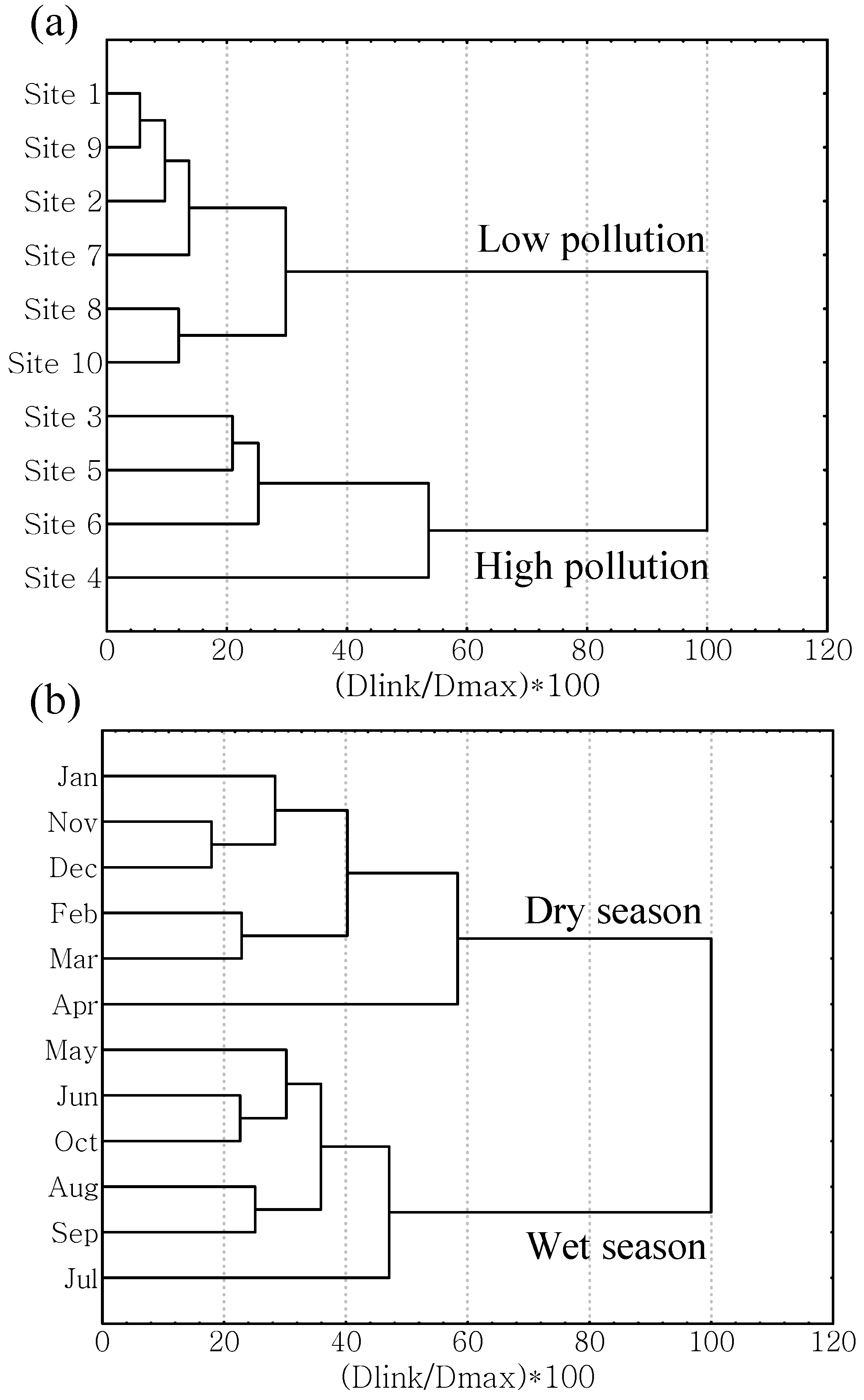
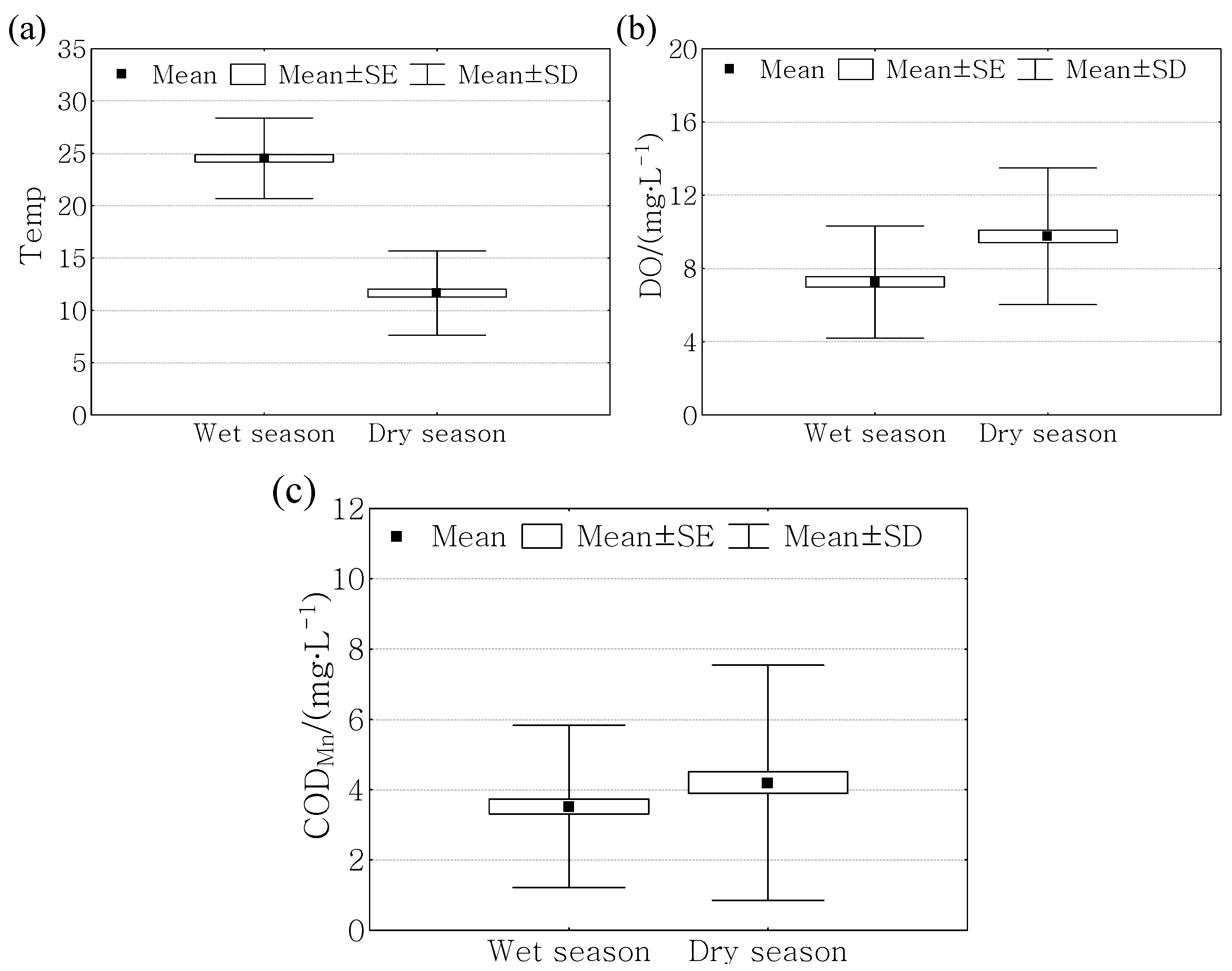
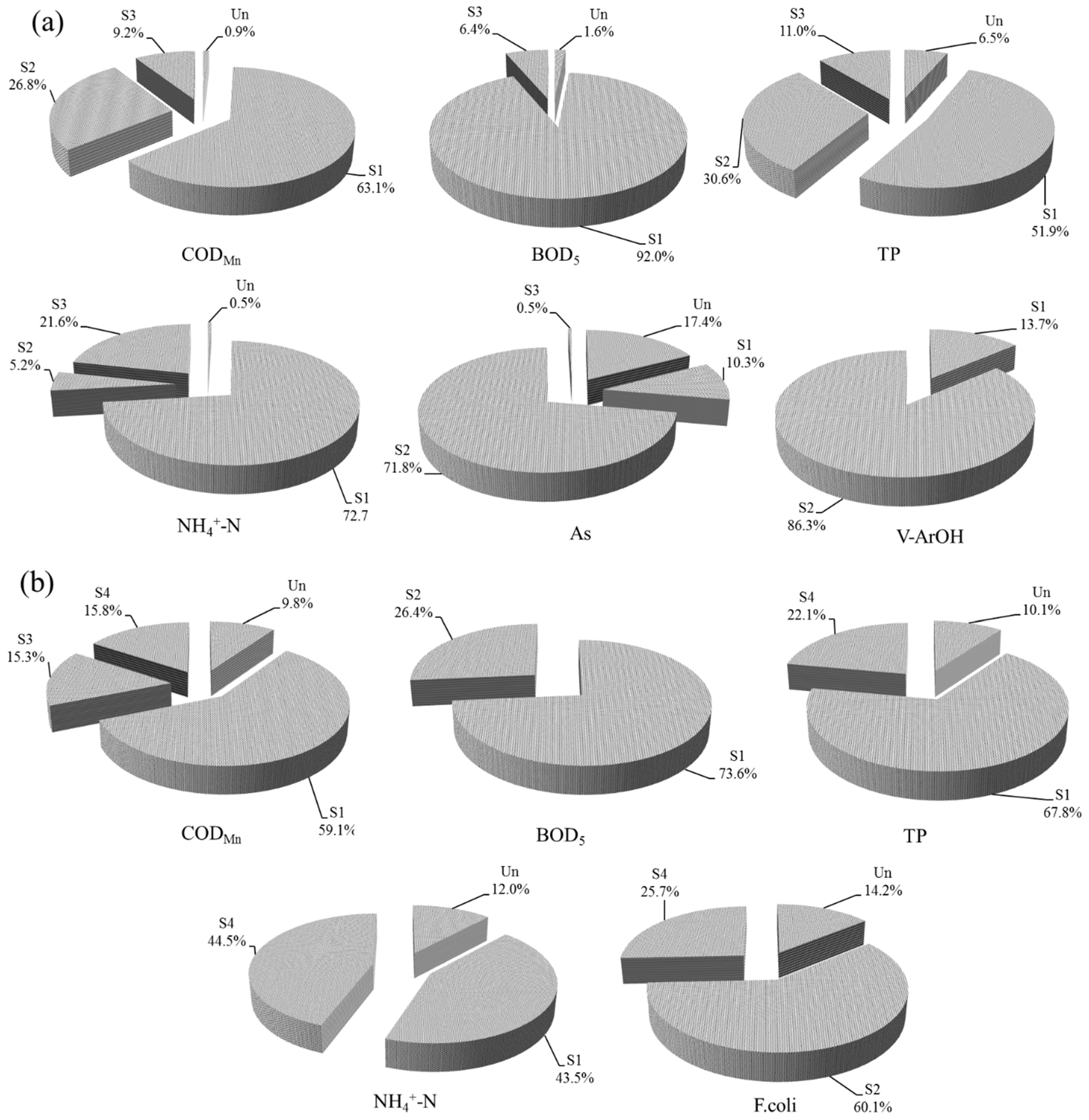
In this study, spatio-temporal variations of water quality and potential pollution sources in Danjiangkou Reservoir Basin were analyzed based on FCA, CA, DA, PCA/FA and APCS-MLR methods. FCA showed that water quality in Jiang River, Shending River, Si River and Jian River has deteriorated, while in other rivers water quality was good. CA divided the ten monitoring sites into two groups (high pollution region and low pollution region) and grouped 12 months into two periods (wet season and dry season). DA showed that pH, COD_Mn, BOD₅, NH₄⁺-N, and F⁻ were the most significant parameters responsible for spatial variations, and Temp, DO, and COD_Mn were the most significant parameters responsible for temporal variations. PCA/FA and APCS-MLR identified four potential pollution types: organic pollution, nutrient pollution, chemical pollution, and natural pollution, and revealed that the study area was primarily influenced by industrial effluent and domestic sewage. Furthermore, the HP region was also influenced by chemical industrial activities and the LP region was also polluted by the sewage from livestock and agriculture. Temporal difference of potential pollution sources in the HP region was significant due to smaller volume of flow in the rivers. Additionally, pollution from agricultural activities was found during the wet season when more nutrient pollutions were discharged into the rivers during irrigation period. This study showed the feasibility and reliability of the combined use of these methods in water environment research. Furthermore, the conclusion would be beneficial to water environment protection and water resources management in the future.

References

1. Iscen, C.F.; Emiroglu, Ö.; Ilhan, S.; Arslan, N.; Yilmaz, V.; Ahiska, S. Application of multivariate statistical techniques in the assessment of surface water quality in Uluabat Lake, Turkey. Environ. Monit. Assess. 2008, 144, 269–276. [Google Scholar] [CrossRef] [PubMed]
2. González, S.O.; Almeida, C.A.; Calderón, M.; Mallea, M.A.; González, P. Assessment of the water self-purification capacity on a river affected by organic pollution: Application of chemometrics in spatial and temporal variations. Environ. Sci. Pollut. Res. 2014, 21, 10583–10593. [Google Scholar] [CrossRef]
3. Bhaduri, B.; Minner, M.; Tatalovich, S.; Harbor, J. Long-term hydrologic impact of urbanization: A table of two models. J. Water Res. Plan. Man. 2001, 127, 13–19. [Google Scholar] [CrossRef]
4. Da Silva Alves, R.I.; de Oliveira Cardoso, O.; de Abreu Tonani, K.A.; Julião, F.C.; Trevilato, T.M.B.; Segura-Muñoz, S.I. Water quality of the Ribeirão Preto Stream, a watercourse under anthropogenic influence in the southeast of Brazil. Environ. Monit. Assess. 2013, 185, 1151–1161. [Google Scholar] [CrossRef] [PubMed]
5. Salve, P.R.; Gobre, T.; Lohkare, H.; Krupadam, R.J.; Bansiwal, A.; Ramteke, D.S.; Wate, S.R. Source identification and variation in the chemical composition of rainwater at coastal and industrial areas of India. J. Atmos. Chem. 2011, 68, 183–198. [Google Scholar] [CrossRef]
6. Mustapha, A.; Aris, A.Z.; Yusoff, F.M.; Zakaria, M.P.; Ramli, M.F.; Abdullah, A.M.; Kura, N.U.; Narany, T.S. Statistical approach in determining the spatial changes of surface water quality at the upper course of Kano River, Nigeria. Water Qual. Expo. Health 2014, 6, 127–142. [Google Scholar] [CrossRef]
7. Shrestha, S.; Kazama, F. Assessment of surface water quality using multivariate statistical techniques: A case study of the Fuji river basin, Japan. Environ. Modell. Softw. 2007, 22, 464–475. [Google Scholar] [CrossRef]
8. Mustapha, A.; Aris, A.Z.; Juahir, H.; Ramli, M.F.; Kura, N.U. River water quality assessment using environmentric techniques: Case study of Jakara River Basin. Environ. Sci. Pollut. Res. 2013, 20, 5630–5644. [Google Scholar] [CrossRef] [Green Version]
9. Kazi, T.G.; Arain, M.B.; Jamali, M.K.; Jalbani, N.; Afridi, H.I.; Sarfraz, R.A.; Baig, J.A.; Shah, A.Q. Assessment of water quality of polluted lake using multivariate statistical techniques: A case study. Ecotox. Environ. Safe. 2009, 72, 301–309. [Google Scholar] [CrossRef]
10. Liou, Y.T.; Lo, S.L. A fuzzy index model for trophic status evaluation of reservoir waters. Water Res. 2005, 39, 1415–1423. [Google Scholar] [CrossRef] [PubMed]
11. Lu, R.S.; Lo, S.L.; Hu, J.Y. Analysis of reservoir water quality using fuzzy synthetic evaluation. Stoch. Environ. Res. Risk Assess. 1999, 13, 327–336. [Google Scholar] [CrossRef]
12. Dahiya, S.; Singh, B.; Gaur, S.; Garg, V.K.; Kushwaha, H.S. Analysis of groundwater quality using fuzzy synthetic evaluation. J. Hazard. Mater. 2007, 147, 938–946. [Google Scholar] [CrossRef] [PubMed]
13. Huang, F.; Wang, X.Q.; Lou, L.P.; Zhou, Z.Q.; Wu, J.P. Spatial variation and source apportionment of water Pollution in Qiantang River (China) using statistical techniques. Water Res. 2010, 44, 1562–1572. [Google Scholar] [CrossRef] [PubMed]
14. Varol, M. Dissolved heavy metal concentrations of the Kralkizi, Dicle and Batman dam reservoirs in the Tigris River Basin, Turkey. Chemosphere 2013, 93, 954–962. [Google Scholar] [CrossRef] [PubMed]
15. Yang, Y.H.; Zhou, F.; Guo, H.C.; Sheng, H.; Liu, H.; Dao, X.; He, C.J. Analysis of spatial and temporal water pollution patterns in Lake Dianchi using multivariate statistical methods. Environ. Monit. Assess. 2010, 170, 407–416. [Google Scholar] [CrossRef] [PubMed]
16. Gridharan, L.; Venugopal, T.; Jayaprakash, M. Assessment of water quality using chemometric tools: A case study of river Cooum, south, India. Arch. Environ. Contam. Toxicol. 2009, 56, 654–669. [Google Scholar] [CrossRef] [PubMed]
17. Papaioannou, A.; Mavridou, A.; Hadjichristodoulou, C.; Papastergiou, P.; Pappa, O.; Dovriki, E.; Rigas, I. Application of multivariate statistical methods for groundwater physicochemical and biological quality assessment in the context of public health. Environ. Monit. Assess. 2010, 170, 87–97. [Google Scholar] [CrossRef] [PubMed]
18. Singh, K.P.; Malik, A.; Sinha, S. Water quality assessment and apportionment of pollution sources of Gomti river (India) using multivariate statistical techniques—A case study. Anal. Chim. Acta 2005, 538, 355–374. [Google Scholar] [CrossRef]
19. Zhang, X.; Wang, Q.S.; Liu, Y.F.; Wu, J.; Yu, M. Application of multivariate statistical techniques in the assessment of water quality in the Southwest New Territories and Kowloon, Hong Kong. Environ. Monit. Assess. 2011, 173, 17–27. [Google Scholar] [CrossRef] [PubMed]
20. Lim, W.Y.; Aris, A.Z.; Praveena, S.M. Application of the chemometric approach to evaluate the spatial variation of water chemistry and the identification of the sources of pollution in Langat River, Malaysia. Arab. J. Geosic. 2013, 6, 4891–4901. [Google Scholar] [CrossRef]
21. Tanrıverdi, Ç.; Alp, A.; Demirkıran, A.R.; Üçkardeş, F. Assessment of surface water quality of the Ceyhan River basin, Turkey. Environ. Monit. Assess. 2010, 167, 175–184. [Google Scholar] [CrossRef]
22. Jha, D.K.; Vinithkumar, N.V.; Sahu, B.K.; Das, A.K.; Dheenan, P.S.; Venkateshwaran, P.; Begum, M.; Ganesh, T.; Devi, M.P.; Kirubagaran, R. Multivariate statistical approach to identify significant sources influencing the physico-chemical variables in Aerial Bay, North Andaman, India. Mar. Pollut. Bull. 2014, 85, 261–267. [Google Scholar] [CrossRef] [PubMed]
23. Pekey, H.; Karakas, D.; Bakoğlu, M. Source apportionment of trace metals in surface waters of a polluted stream using multivariate statistical analyses. Mar. Pollut. Bull. 2004, 49, 809–818. [Google Scholar] [CrossRef] [PubMed]
24. Miller, S.L.; Anderson, M.J.; Daly, E.P.; Milford, J.B. Source apportionment of exposures to volatile organic compounds. I. Evaluation of receptor models using simulated exposure data. Atmos. Environ. 2002, 36, 3629–3641. [Google Scholar] [CrossRef]
25. Yang, L.P.; Mei, K.; Liu, X.M.; Wu, L.S.; Zhang, M.H.; Xu, J.M.; Wang, F. Spatial distribution and source apportionment of water pollution in different administrative zones of Wen-Rui-Tang (WRT) river watershed, China. Environ. Sci. Pollut. Res. 2013, 20, 5341–5352. [Google Scholar] [CrossRef]
26. Su, S.L.; Li, D.; Zhang, Q.; Xiao, R.; Huang, F.; Wu, J.P. Temporal trend and source apportionment of water pollution in different functional zones of Qiantang River, China. Water Res. 2011, 45, 1781–1795. [Google Scholar] [CrossRef] [PubMed]
27. Mavukkandy, M.O.; Karmakar, S.; Harikumar, P.S. Assessment and rationalization of water quality monitoring network: A multivariate statistical approach to the Kabbini River (India). Environ. Sci. Pollut. Res. 2014, 21, 10045–10066. [Google Scholar] [CrossRef]
28. Palma, P.; Alvarenga, P.; Palma, V.L.; Fernandes, R.M.; Soares, A.M.V.M.; Barbosa, I.R. Assessment of anthropogenic sources of water pollution using multivariate statistical techniques: A case study of the Alqueva’s reservoir, Portugal. Environ. Monit. Assess. 2010, 165, 539–552. [Google Scholar] [CrossRef] [PubMed]
29. Li, S.Y.; Gu, S.; Liu, W.Z.; Han, H.Y.; Zhang, Q.F. Water quality in relation to the land use and land cover in the Upper Han River basin, China. Catena 2008, 75, 216–222. [Google Scholar] [CrossRef]
30. Li, S.Y.; Cheng, X.L.; Xu, Z.F.; Han, H.Y.; Zhang, Q.F. Spatial and temporal patterns of the water quality in the Danjiangkou Reservoir, China. Hydrolog. Sci. J. 2009, 54, 124–134. [Google Scholar] [CrossRef]
31. Vega, M.; Pardo, R.; Barrado, E.; Deban, L. Assessment of seasonal and polluting effects on the quality of river water by exploratory data analysis. Water Res. 1998, 32, 3581–3592. [Google Scholar] [CrossRef]
32. Osman, R.; Saim, N.; Juahir, H.; Abdullah, M.P. Chemometric application in identifying sources of organic contaminants in Langat river basin. Environ. Monit. Assess. 2012, 184, 1001–1014. [Google Scholar] [CrossRef] [PubMed]
33. Simeonov, V.; Stratis, J.A.; Samara, C.; Zachariadis, G.; Voutsa, D.; Anthemidis, A.; Sofoniou, M.; Kouimtzis, Th. Assessment of the surface water quality in Northern Greece. Water Res. 2003, 37, 4119–4124. [Google Scholar] [CrossRef] [PubMed]
34. Alberto, W.D.; del Pilar, D.M.; Valeria, A.M.; Fabiana, P.S.; Cecilia, H.A.; de Los Angeles, B.M. Pattern recognition techniques for the evaluation of spatial and temporal variation in water quality. A case study: Suquia river basin (Cordoba Argentina). Water Res. 2001, 35, 2881–2894. [Google Scholar] [CrossRef] [PubMed]
35. Liu, C.W.; Lin, K.H.; Kuo, Y.M. Application of factor analysis in the assessment of groundwater quality in a blackfoot disease area in Taiwan. Sci. Total Environ. 2003, 313, 77–89. [Google Scholar] [CrossRef] [PubMed]
36. Singh, K.P.; Malik, A.; Kumar, R.; Saxena, P.; Sinha, S. Receptor modeling for source apportionment of polycyclic aromatic hydrocarbons in urban atmosphere. Environ. Monit. Assess. 2008, 136, 183–196. [Google Scholar] [CrossRef] [PubMed]
37. Lattin, J.M.; Carroll, J.D.; Green, P.E. Analyzing Multivariate Data; Duxbury: New York, NY, USA, 2003. [Google Scholar]
38. Kowalkowski, T.; Zbytniewski, R.; Szpejna, J.; Buszewski, B. Application of chemometrics in river water classification. Water Res. 2006, 40, 744–752. [Google Scholar] [CrossRef] [PubMed]
39. Varol, M.; Gökot, B.; Bekleyen, A.; Şen, B. Spatial and temporal variations in surface water quality of the dam reservoirs in the Tigris River Basin, Turkey. Catena 2012, 92, 11–21. [Google Scholar] [CrossRef]
40. Zilberbran, M.; Rosenthal, E.; Shachnai, E. Impact of urbanization on hydrochemical evolution of groundwater and on unsaturated-zone gas composition in the coastal city of Tel Aviv, Israel. J. Contam. Hydrol. 2001, 50, 175–208. [Google Scholar] [CrossRef] [PubMed]
41. Jain, C.K. A hydro-chemical study of a mountainous watershed: The Ganga, India. Water Res. 2002, 36, 1262–1274. [Google Scholar] [CrossRef] [PubMed]
42. Juahir, H.; Zain, S.M.; Yusoff, M.K.; Hanidza, T.I.T.; Armi, A.S.M.; Toriman, M.E.; Mokhtar, M. Spatial water quality assessment of Langat River Basin (Malaysia) using environmetric techniques. Environ. Monit. Assess. 2011, 173, 625–641. [Google Scholar] [CrossRef] [PubMed]
43. Kannel, P.R.; Lee, S.; Lee, Y.S. Assessment of spatial-temporal patterns of surface and ground water qualities and factors influencing management strategy of groundwater system in an urban river corridor of Nepal. J. Environ. Manag. 2008, 86, 595–604. [Google Scholar] [CrossRef]
44. Phillips, D.J.H. Arsenic in aquatic organisms: A review, emphasizing chemical speciation. Aquat. Toxicol. 1990, 16, 151–186. [Google Scholar] [CrossRef]
45. Zhang, Y.; Guo, F.; Meng, W.; Wang, X.Q. Water quality assessment and source identification of Daliao River Basin using multivariate statistical methods. Environ. Monit. Assess. 2009, 152, 105–121. [Google Scholar] [CrossRef] [PubMed]