

Spatially Consistent Drought Hazard Modeling Approach Applied to West Africa

University of Clermont Auvergne, CNRS, IRD, CERDI, F-63000 Clermont-Ferrand, France
*
Author to whom correspondence should be addressed.
Water 2023, 15(16), 2935; https://doi.org/10.3390/w15162935
Submission received: 2 July 2023
/
Revised: 8 August 2023
/
Accepted: 9 August 2023
/
Published: 14 August 2023
(This article belongs to the Special Issue Water Management in Arid and Semi-arid Regions)
Abstract
:A critical stage in drought risk assessment is the measurement of drought hazard, the probability of occurrence of a potentially damaging event. The standard approach to assess drought hazard is based on the standardized precipitation index (SPI) and a drought intensity classification established according to a fixed set of SPI values. We show that this method does not allow for the assessment of region-specific hazards, and we propose an alternative method based on the extreme value theory. We model precipitation using an extreme value mixture model, with a normal distribution for the bulk, and a generalized Pareto distribution for the upper and lower tails. The model estimation allows us to identify the threshold value below which precipitation can be qualified as extreme. The quantile function is used to measure the intensity of each category of droughts and calculate the drought hazard index (DHI). By construction, the DHI value varies according to the specific characteristics of the left tail of the precipitation distribution. To test the relevance of our approach, we estimate the DHI over a gridded set of rainfall data covering West Africa, a large and climatically heterogeneous region. The results show that our mixture model fits the data better than the model used for SPI calculation. In particular, our model performs better to identify extreme precipitation in the left tail of the distribution. The DHI map highlights clusters of high drought hazard located in the central part of the region under study.
1. Introduction
This study belongs to the strand of literature dedicated to drought risk assessment and management—e.g., [1,2,3,4]. In sub-Saharan Africa, drought is a major and recurrent threat to human life, economic activity, and the environment [5]. As rainfed agriculture is the dominant production system, dry spells may have a significant impact on the agricultural sector, which makes up a large percentage of the gross domestic product of these low-income countries. Despite the pervasive impact of droughts in Africa, drought risk management strategies have long been limited to ex-post emergency responses [6]. This has led the United Nations Convention to Combat Desertification to plead for urgent action at the global, regional and national levels to establish a strategic framework for drought risk management in Africa [7]. In order to define such a consistent framework and enhance drought resilience, one essential prerequisite is to clearly identify and understand the drought risk components [8,9].
The risk associated with a natural hazard is defined as the potential loss resulting from the hazard. It is commonly viewed as the combination of three components: hazard, exposure, and vulnerability [2,10,11]. Hazard, the first component of risk, can be defined as the probability of the occurrence of a potentially damaging event [12]. The difficulty in measuring drought hazard comes from the multiplicity of drought definitions. There is no single definition of drought, and drought assessment is necessarily region- and impact-specific—e.g., [13,14,15]. Like other natural hazards, droughts can be characterized in terms of their intensity, frequency, duration, location, and timing [16]. However, droughts differ from other natural hazards in many respects.
Drought is a socioeconomic construct whose definition relates to its impact. The climatological community has defined four types of drought: meteorological drought, agricultural drought, hydrological drought, and socioeconomic drought [14,16]. Meteorological drought is a relative rather than an absolute concept, defined as a prolonged dry period in the natural climate cycle of a region. Meteorological droughts can occur in any part of the world, whether arid or wet, and are measured by a departure from normal precipitation over some specified period of time [17]. Meteorological droughts are commonly assessed using the standardized precipitation index (SPI) of McKee, T. et al. [18]. Agricultural droughts originate from soil water depletion during a specific growing stage of a crop, leading to reduced yields. A commonly used index to assess agricultural droughts is the standardized precipitation evapotranspiration index (SPEI), which combines precipitation and evapotranspiration indicators to measure the soil moisture level [19]. Hydrological drought refers to persistently low surface or subsurface water supplies in streams, rivers, reservoirs, or groundwater. The Palmer drought severity index [20] is used to assess this type of long-term drought, which usually results from a prolonged meteorological drought. The index combines temperature and water balance indicators. Socioeconomic drought occurs when the demand for water exceeds the supply for domestic use or economic activity, for instance, in the hydroelectric energy production sector or irrigation [6].
All drought types originate from a deficiency of precipitation, i.e., a meteorological drought that then propagates to other drought types (agricultural, hydrological, or socioeconomic) [17]. This is why drought hazard analyses at the global level generally focus on this type of drought and use the standardized precipitation index to assess drought hazard. To calculate the SPI, the raw precipitation data are fitted to an incomplete Gamma distribution and then transformed into Gaussian equivalents with zero mean and variance equal to one (for more computational details, see [21,22]). Therefore, SPI values are dimensionless, are comparable across regions with different climatic regimes, and offer a readily interpretable measure of drought intensity. Establishing a drought classification based on the intensity thresholds becomes straightforward, and the drought hazard index (DHI) is computed as the weighted sum of the frequency of the occurrence of each drought category—e.g., [23,24]. The reference set of drought intensity thresholds used in the literature is that of McKee, T. et al. [18], who distinguish four drought categories, from mild to severe, according to a fixed set of SPI values (see also [25,26]).
Calculating the frequency and intensity of droughts from a standardized index offers the advantage of simplicity for analyzing drought hazard, but as a result of the standardization process, each drought intensity category has the same probability of occurrence, and the theoretical value of the drought hazard index is the same whatever the geographical location [27]. Another drawback is that standardization results in a loss of information on rare events in the distribution tails, which are precisely the most important to catch in risk analysis.
More recent works draw on the extreme event theory (EVT) and use the Peaks Over Threshold (POT) method introduced by Pickands, J. [28] to estimate the distribution tails of climatic or hydrological variables. According to the Pickands–Balkema–De Haan theorem [28,29], the distribution of excesses above a high-enough threshold can be approximated by a distribution of the generalized Pareto family (see also [30,31]. The main difficulty in applying the POT method lies in the choice of the threshold, which impacts the parameter estimates and quantile inferences [32].
The choice of the threshold can be based on the physical characteristics of the phenomenon under study, for instance, in flood frequency analysis—e.g., [33], but most of the time, the choice of the threshold remains highly subjective. A common practice, the so-called fixed threshold approach, consists of setting the threshold at a fixed quantile level for all precipitation series. For instance, Kim, J.E. et al. [34] chose the threshold level within the 70th and 95th percentiles so as to generate the desired number of droughts. Burke, E.J. et al. [35], using the POT approach, set the threshold to the 94th percentile of monthly drought indexes. Less subjective methods have been developed to estimate the threshold and to account for uncertainty in estimates (see Scarrott, C. and MacDonald, A. [36] for a review of threshold estimation approaches and Langousis et al. [37] for application to rainfall data).
In this paper, we propose to use an extreme value mixture model, with a normal distribution for the bulk and a generalized Pareto distribution (GPD) for the upper and lower tails, to model precipitation. This model is more flexible and fits the data better than the Gamma model usually used for SPI calculation. It allows us to estimate the threshold below which precipitation can be qualified as extreme, as well as the threshold value defining drought categories according to severity. The great advantage of this approach is that this set of thresholds is estimated rather than imposed and is specific to each geographical location. Another advantage of our method is that it provides an estimation of the drought thresholds in the same unit as the raw data, allowing for the implementation of an operational drought monitoring system. Finally, the Drought Hazard Index can be measured more precisely. By construction, its value varies from one location to another, depending on the specific characteristics of each rainfall distribution.
To test the relevance of our approach to drought hazard estimation, we work on a gridded set of rainfall data covering West Africa from January 1901 to December 2020. Although the study area is limited, it includes a wide range of climatic zones. To catch potentially disastrous droughts and to facilitate comparisons with the standard approach of drought classification and DHI evaluation, we focus on meteorological droughts measured from cumulated annual rainfall levels. For ease of interpretation, most of the results are provided in the form of maps.
2. Data and Study Area
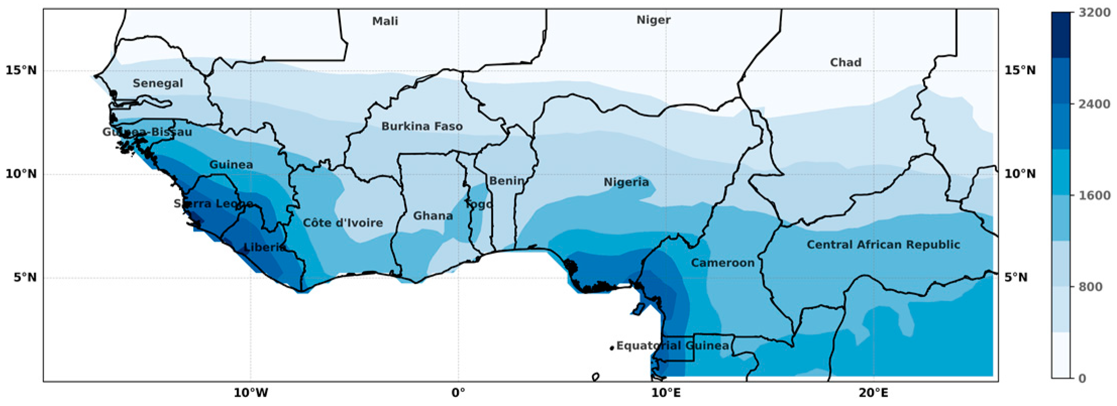
The region under study is located between latitudes 0 and 18° N and longitude 20° W and 20° E (Figure 1). This area is centered in West Africa but also includes a part of Central Africa. The rainfall patterns in this region are determined by the monsoon system and topography. The region encompasses three major climatic areas and several climate transition zones that cross the region from east to west, forming virtually parallel strips from the Tropic of Cancer to the Equator.
In the north of the studied area, above latitude 18° N, the climate is either semi-desert, of the northern Sahelian type, or desert. The rainy season is concentrated over one or two months, and the average annual rainfall varies from 300 mm to less than 100 mm. Further south, the tropical climate is characterized by very distinct dry and wet seasons. The length of the wet season and the amount of annual rainfall allows for distinguishing three types of tropical climates. The Sahelian, or semi-arid tropical climate, lies between latitudes 12° N and 18° N; the dry season lasts seven to ten months, and the average annual rainfall varies between 300 and 700 mm. The Sudanian, or pure tropical, climate corresponds to a dry season of five to six months, with the average annual rainfall between 700 and 1000 mm (1200 mm on the Senegalese coast). The Guinean, or transitional tropical, climate corresponds to a shorter dry season, from four to five months, and an average annual rainfall above 1000 mm. The transitional equatorial and equatorial climates lie below 10° N over the countries of the Gulf of Guinea. The annual precipitations are abundant, generally above 1000 mm with a bimodal distribution (two dry seasons). However, the rainfall distribution is quite heterogeneous in this area. The climate is very humid, with an annual rainfall above 2500 mm in the coastal regions of Guinea, Cameroon, and Gabon, which are characterized by mountainous relief. By contrast, the Dahomey Gap, which includes parts of Ghana, Togo, and Benin and has an annual rainfall total of 1000 to 1200 mm, is abnormally dry for the region (see Figure 1).
During the twentieth century, the region experienced several periods of intense drought [7]. Widespread and severe droughts were recorded in the 1910s and 1940s in the Sahelian region. More severe droughts ravaged the region from 1968 to 1974 and during the early- and mid-1980s. These droughts caused famines, massive displacements, and considerable loss of human life. The tropical part of West Africa was also affected by these two major droughts but in a more heterogeneous way. More recently, in the years 2010–2011, a new drought wave affected the whole region from the Sahelian band to the northern coast of the Gulf of Guinea but with a very variable intensity.
To catch droughts with potentially damaging consequences on the economies and populations of the region studied, we calculate annual rainfall totals. In the Sudano–Sahelian area where rainfall is concentrated over June to September, the annual rainfall accumulation corresponds to the seasonal accumulation. In case of a deficit, the entire year’s harvest is at risk. In the southern part of the area, close to the equator, rains are bimodal so that a “normal” (equal to mean) annual rainfall level can mask a drought during one of the two rainfall seasons. Without ignoring the potential compensation between the rainy seasons, we assume that when the annual rainfall deficit is high, the year’s production is compromised, whatever the geographical area or intra-annual rainfall distribution.
The rainfall data come from the Climatic Research Unit at the University of East Anglia (https://www.uea.ac.uk/groups-and-centres/climatic-research-unit, accessed on 28 March 2022). We use the gridded time-series of monthly rainfall totals at 0.5° × 0.5° latitude/longitude resolution for the period January 1901–December 2020. The data were extracted from the revised January 2021 version of the dataset referred to as CRU TS4.05. The construction of the CRU dataset is detailed in [38]. Before proceeding to the estimations, the database had to be cleaned. Prior to 1930, numerous annual rainfall data that repeat for two or more consecutive years were detected, especially for cells located in the northern part of the region. These observations were dropped from the dataset, as well as other repetitions detected after 1930. As a consequence, the starting date of the rainfall series and the number of observations in each series may vary from cell to cell.
3. The Extreme Value Mixture Model
There is a wide range of extreme event mixture models combining a generalized Pareto distribution (GPD) for the upper tail with a parametric or nonparametric model for the central distribution (see a review in [36,39]). We are interested in mixture models where the threshold is a parameter to be estimated, along with the other model’s parameters. Apart from providing an objective estimation of the threshold, the main advantage of parametric mixture models is that they provide an analytical expression for the data, which can be used for simulations. Moreover, parametric mixture models can be easily applied to large data sets.
However, the choice of the model for the bulk is a concern, since a poor specification of the central distribution will impact the threshold estimation and the tail fit [36]. A non-parametric model for the bulk, such as the smooth kernel density estimator proposed by MacDonald, A. et al. [40], offers more flexibility and robustness of the tail fit to that of the bulk. In return, non-parametric models are very computationally intensive, which is an obstacle to their application to a large data set such as ours.
Therefore, we consider a two-tail model, combining a GPD for each tail and a parametric form for the central distribution. This model is an extension of Behrens, C.N. et al.’s [41] two distributions mixture model. The GPD–Normal–GPD (GNG) mixture model was used, for instance, by Mendes, B. and Lopes, H.F. [42], and by Zhao, X. et al. [43] on financial data. Solari, S. and Losada, M.A. [39] also apply this model to precipitation and flow data but with a lognormal for the central distribution.
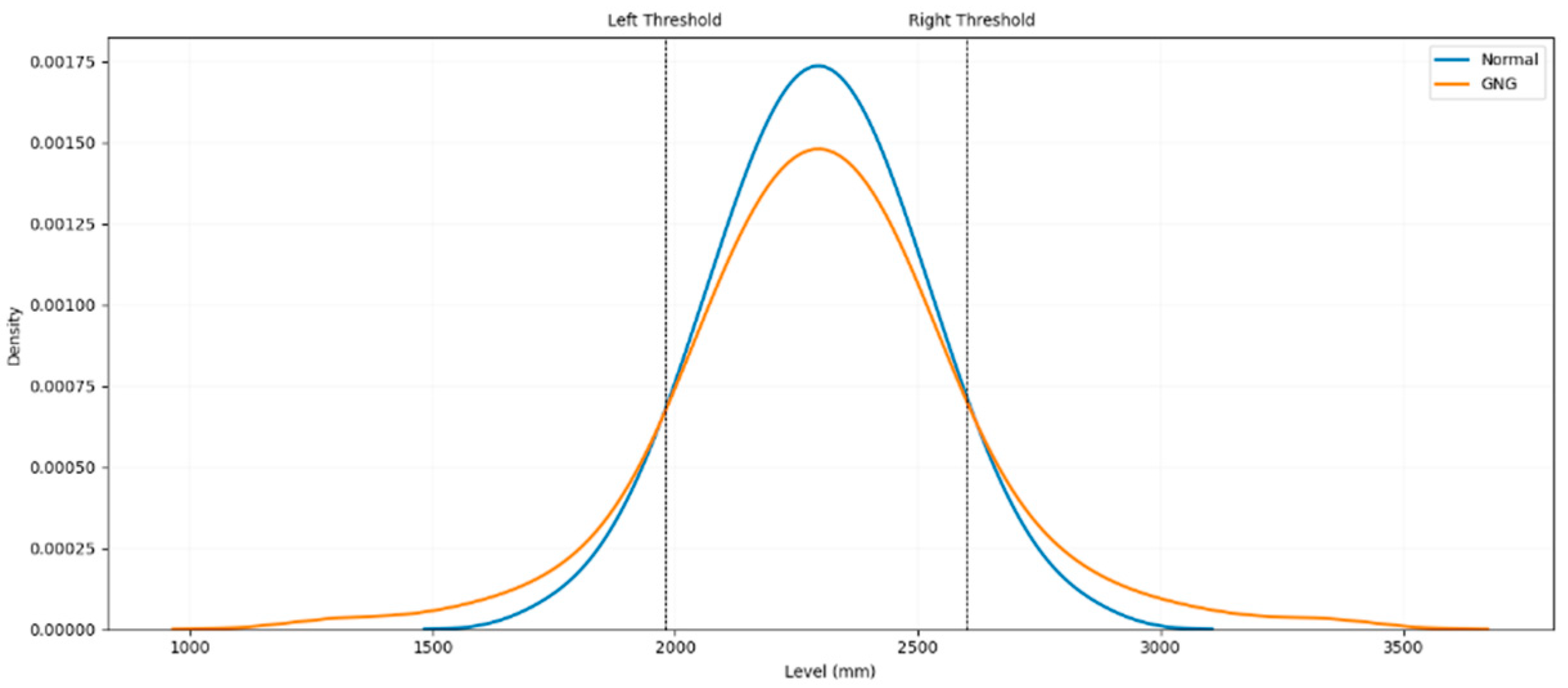
The GNG model allows for asymmetry in the left and right thresholds and for the parameters of the right and left GDPs to differ. In the absence of any theoretical justification, we chose a Gaussian for the central part of the distribution, considering like Tukey, J.W. [44], that all distributions are normal in the middle (Winsor’s principle). This is also the hypothesis made by Mendes, B. and Lopes, H.F. [42] for their extreme value mixture model.
Let be a sequence of independent and identically distributed observations; the cumulative distribution function for the standard GNG mixture model is given by Hu, Y. and Scarrott, C. [45]:
is the normal cumulative distribution function with mean m and variance s2; is the conditional GPD cumulative distribution function with location parameter u, scale σ, and shape ξ. The subscripts l and r for the GDP parameters are for the left and right tails of the distribution. In this specification, the tail fraction below the lower threshold, and the tail fraction above the upper threshold, are two implicit parameters defined by the normal bulk model: and The authors of [45] refer to this model as the “bulk model approach”. To reduce the estimation bias related to a potential misspecification of the central distribution, we adopt the more general parametrized tail fraction approach of [40]. In this specification, and are extra parameters to be estimated so that the tail fit is more robust to the bulk model [45]. The cumulative distribution function is given by (2):
The conditional GPD cumulative distribution function up to the lower threshold is given by:
for all if ; for all if . .
The conditional GPD cumulative distribution function above the upper threshold is given by:
for all if ; for all if. .
The shape parameter (ξ) determines the tail behavior: if ξ = 0, the distribution has an exponential, light-tailed distribution and belongs to the Gumbel family; if ξ < 0, the distribution has a short, bounded tail and belongs to the Weibull family; if ξ > 0, the distribution has a heavier tail and belongs to the Fréchet family (see, for instance, [32]).
The vector of parameters to be estimated is , with m and s2 being the mean and variance of the normal bulk distribution; and are the location parameters, defining, respectively, the lower and upper tail thresholds; σl and σr are the scale parameters; and are the shape parameters; and are the tail fraction, representing, respectively, the probability of being above the upper threshold and below the lower threshold. We use for estimations the maximum likelihood estimator in the Evmix R package developed by Hu, Y. and Scarrott, C. [45].
As an illustration, Figure 2 depicts the density of a Gaussian law and of a mixture with two Weibull distributions for the tails and a normal for the bulk. In this figure, the density is continuous at the thresholds, although it is not a necessary condition. In estimations, we do not impose a continuity constraint at the thresholds in the probability density function. Imposing continuity induces a dependence between the bulk and tail estimates and may have an adverse effect on model identification if the bulk model is poorly specified [45].
4. Results
We, first, present the results of the mixture estimates and then the calculation of the drought hazard index.
4.1. Main Results from the Mixture Model
The mixture model is estimated separately for each grid cell using the annual rainfall data from 1901 to 2020. As a rule, we present only the estimation results for the left tail of the distribution, corresponding to drought events.
4.1.1. Stationarity Tests
The Pickands theorem applies to a series of independent and identically distributed random variables but can be extended to a stationary time series [30,31]. The stationary hypothesis is questionable for climatic data, in particular precipitation data, which may exhibit a trend, cycles, or breaks. Over the period under study, the Sahel region experienced a great drought in 1968–1973, which marked the end of a wet period and the beginning of a long dry period that lasted at least until the late 1990s. The occurrence of a structural break in the precipitation level at the end of the 1960s was documented by many authors—e.g., [46,47]. However, the return of more abundant precipitation at the beginning of the 2000s tends to show that rainfall evolution in this more recent period is part of a long cycle process [48,49,50]. Therefore, the validity of stationarity tests is questionable. As Panthou, G. et al. [48] point out, the results of stationarity tests on climate series depend crucially on the temporal depth of the data. A rainfall series can be non-stationary over several decades and stationary over a longer period and vice versa.
The objective here is not to conduct an in-depth analysis of the behavior of the rainfall series but rather to assess the scope of our results. Therefore, we implement three tests: the Augmented Dickey Fuller (ADF) unit root test, Pettitt’s [51] non-parametric change point test, and a test for short-term dependence in the POT series.
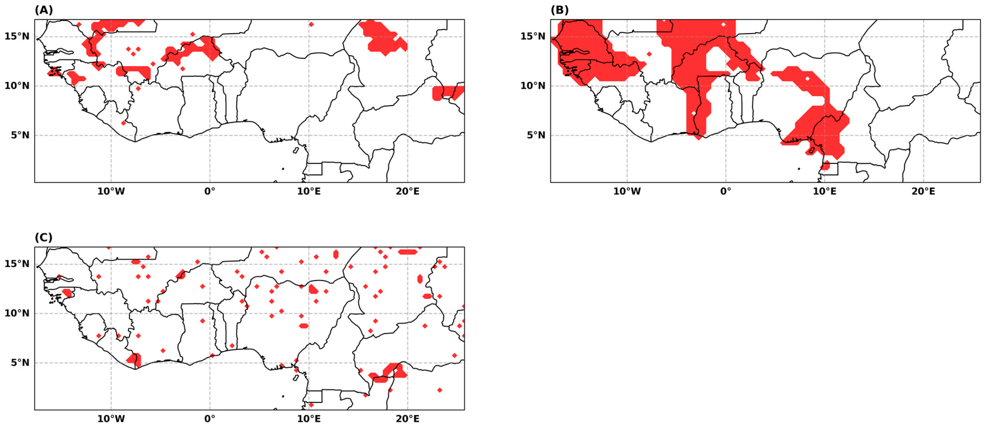
The ADF test rejects at the 5% level the stochastic trend hypothesis for the vast majority of the sample series (Figure 3A). A failure to reject the unit root hypothesis may be due to a persistent break in level that can be detected by the Pettit test, which shows that a break in mean precipitation occurred at the end of the 1960s in some parts of the study area. However, this phenomenon is not widespread but confined to some relatively limited geographical areas (Figure 3B). The results of the autocorrelation tests on the POT series are encouraging: the independence hypothesis is not rejected, with only a few exceptions (Figure 3C). The time depth of our data (120 yearly observations) does not allow us to estimate the model before and after the break date nor to estimate the model on a moving window, as in [52]. Consequently, the consistency of the parameter estimates may be an issue, and the estimation results of the mixture model will have to be considered with caution for the series displaying a break in mean.
4.1.2. Goodness-of-Fit Assessments
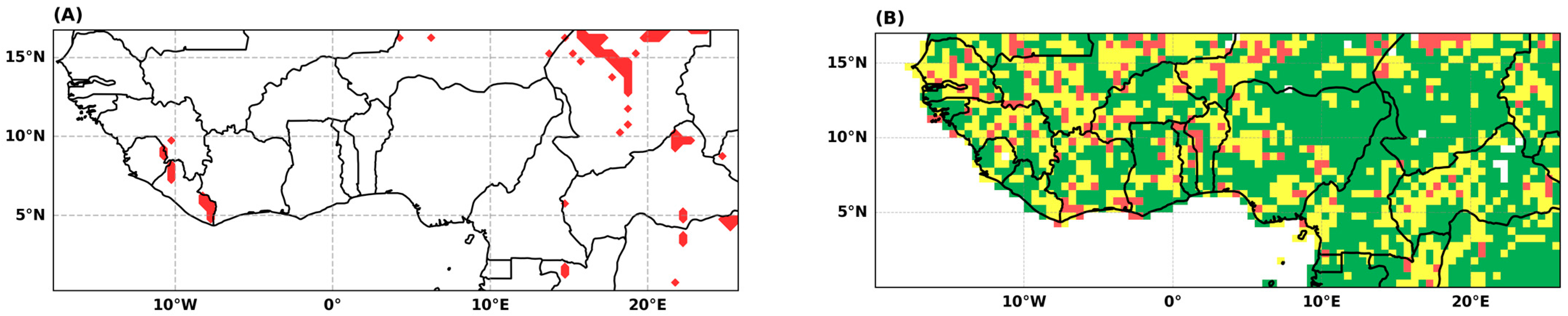
Based on the Kolmogorov–Smirnov (KS) goodness-of-fit test, the estimated mixture model demonstrates a satisfactory representation of the data for the majority of the sample (Figure 4A). The KS test indicates a rejection of the equality between the empirical and mixture cumulative distribution functions (CDF) in only 3.5% of cases. Additionally, the chi-square test reveals a rejection of the null hypothesis, implying a significant difference between the observed and expected values in only 1.7% of cases. Comparing the accuracy of the GNG mixture model and the gamma distribution, which is employed for calculating the SPI, using the Root Mean Square Error (RMSE), it is observed that the GNG mixture model outperforms the gamma distribution in 62.9% of cases. To statistically examine whether the prediction errors from the GNG and the gamma distributions are significantly different, we conduct Diebold and Mariano’s test with a correction for small-sample bias [53,54]. Based on the absolute error loss criterion, the test results presented in Figure 4B demonstrate that the GNG mixture model exhibits superior predictive accuracy compared to the gamma distribution in 57.5% of cases. Conversely, the gamma distribution demonstrates better predictive accuracy in only 8% of cases. Thus, it can be concluded that the GNG model’s accuracy is equal to or higher than that of the gamma distribution in 92% of locations. When considering the square error loss criterion, the results of the Diebold and Mariano test, although not as favorable, still support the superiority of the GNG model, with its accuracy being equal to or higher than that of the gamma distribution in 77% of locations.
4.1.3. The GPD Parameters
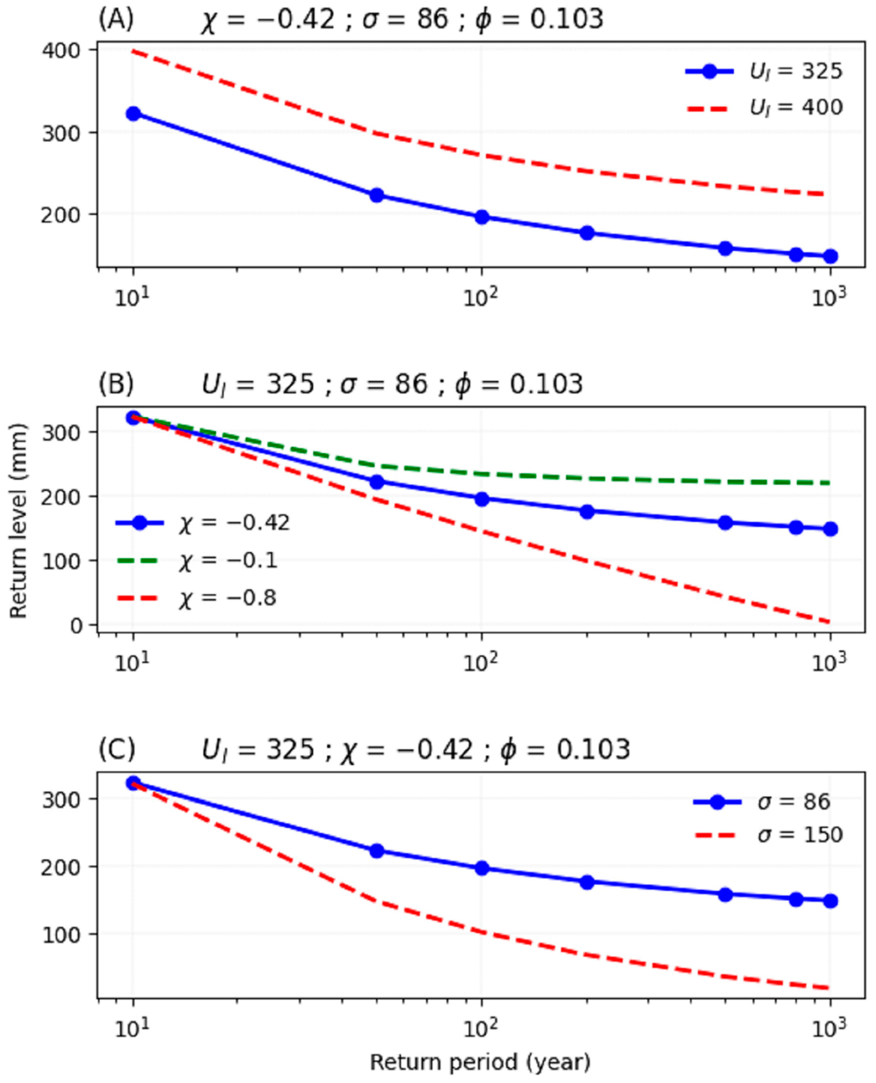
The value of the parameters of the left GPD provides information on the return level of extreme droughts: the intensity of the precipitation deficit increases with the scale () and the shape () parameters and decreases when the location parameter () increases (see return level plots, Figure A1 in Appendix A, and see Appendix B for an analysis of the uncertainty and sensitivity of the model’s parameters).
The location parameter, which defines the threshold for extreme drought, exhibits a similar trend along latitudes as the annual precipitation. This enables spatial comparisons to be made, the location parameter is expressed as z-score: , with and as the mean and standard deviation of annual rainfall, respectively, calculated over the entire period (Figure 5A). The standardized threshold value quantifies the severity of the precipitation shortfall at which a dry period can be classified as an extreme drought. A lower standardized threshold value indicates a greater intensity of extreme droughts. Figure 5A shows a large heterogeneity in threshold values, with spatially dispersed clusters of low (red cells) and high (yellow cells) values.
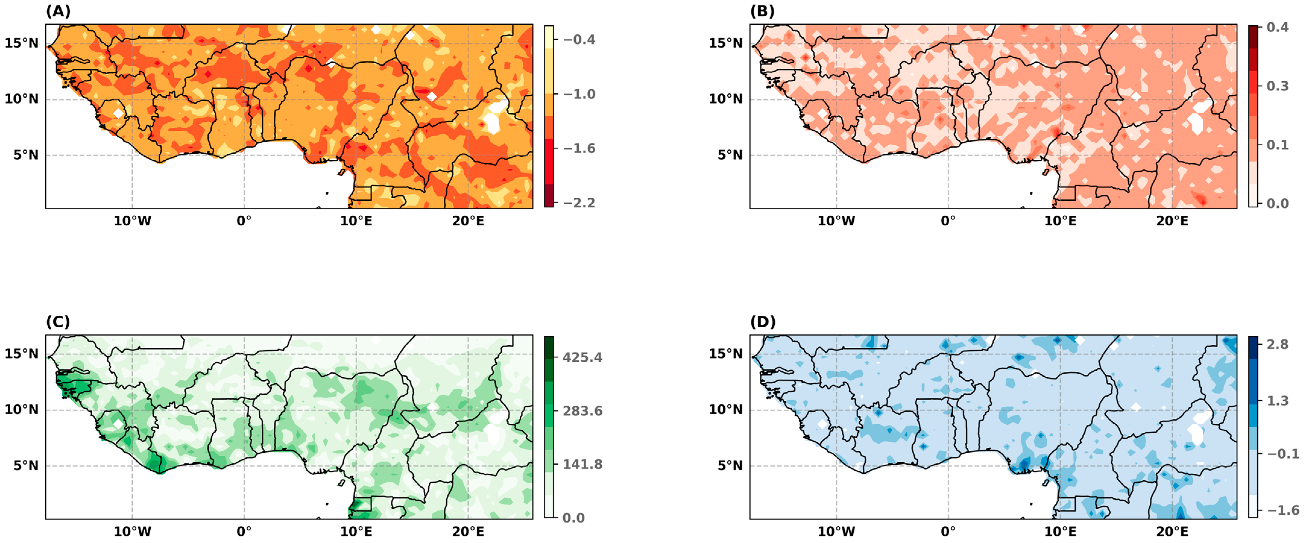
By contrast, the probability of non-exceedance of the extreme drought threshold, or tail fraction, (ϕul), is evenly distributed over the entire area (Figure 5B). On average, the tail fraction equals 10.5%, meaning that a drought that can be qualified as extreme has a return period of approximately 10 years. The combination of the threshold value and the tail fraction shows that the intensity of the rainfall deficit characterizing an extreme drought varies greatly within the region, while this type of event has the same return period (9 years). Figure 5C shows the scale parameter () of the left GPD. The scale parameter is the gradient of the return period curve at the return period of the threshold: the higher the scale parameter, the lower the precipitation level of extreme rare events, all things being equal. Figure 5D displays the shape parameter (). In over 77% of instances, the estimated shape parameter is negative, indicating that the distribution of precipitation has a compact left tail with a defined boundary.
Analyzing these parameters separately does not allow us to identify the area most at risk. One way to summarize the information contained in the distribution tail is to calculate the DHI.
4.2. The Drought Hazard Measurement
4.2.1. The Standard Approach of Drought Hazard
Drought hazard is commonly defined as the combination of the intensity and frequency of droughts and is estimated from the SPI and [18]’s drought intensity classification (Table 1). The drought intensity classification is established according to a fixed set of SPI values, and the drought intensity is caught through fixed weights. The probability of the occurrence of a drought of a given category (ϕi) is the same whatever the geographical location and statistical characteristics of the raw data, but the empirical frequency (fi) may differ from one location to another. The DHI is given by:
is the weight assigned to droughts of category i. is the empirical frequency of droughts of category , namely, the number of drought events of category recorded during the period divided by the number of observations in the period.
We compute the DHI from Equation (5) alternatively using the standard SPI-based approach and the GNG mixture-based approach. In the SPI approach, the thresholds used to distinguish the different drought categories are given in Table 1, column 3. We use the percentiles corresponding to these thresholds values (Table 1, column 4) and the quantile function of the GNG distribution to compute the thresholds of the mixture model. Thus, the theoretical probability of the occurrence of the four drought categories (ϕi) is the same in both approaches, SPI and GNG (Table 1, column 5). According to this drought classification and weighting system, the theoretical value of the DHI, calculated using the theoretical occurrence probability of drought, is 0.24 in both models. If the empirical value of the DHI, calculated using the empirical drought frequency, differs from its theoretical value, it means that the model does not fit the data well.
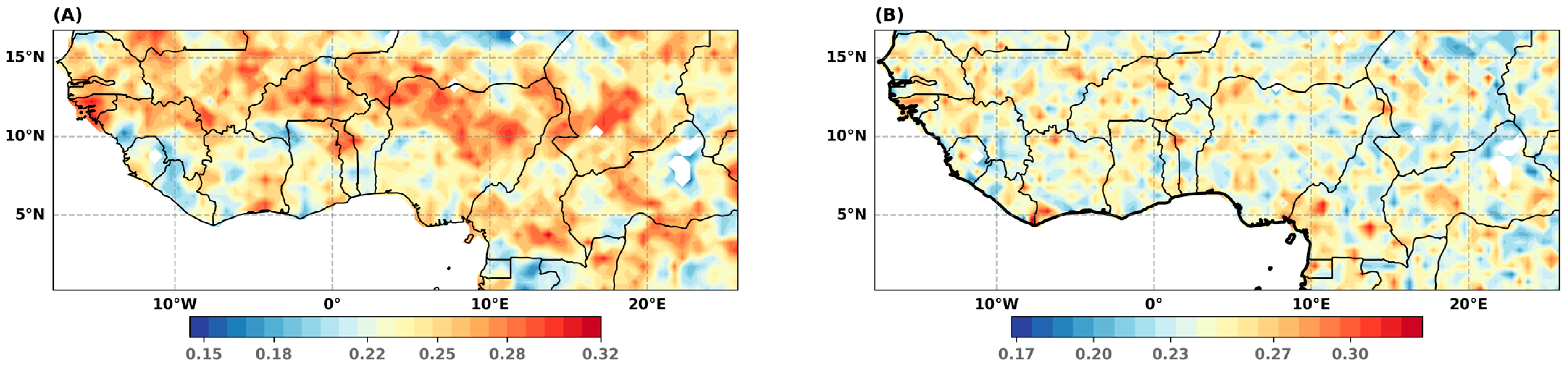
The DHI maps are given by Figure 6A, B. On average, over the whole sample, the DHI calculated from the SPI and GNG models are very close to its theoretical value (respectively, 0.243 and 0.246 vs. 0.24). However, the SPI model underestimates the probability of the occurrence of moderate droughts (7.9% vs. 9.2%) and overestimates that of extreme droughts (2.9% vs. 2.27%). As expected, the SPI model is less efficient than the GNG model in predicting extreme droughts.
Looking at the spatial distribution of the DHI, a structure emerges when the drought hazard is calculated from the SPI (Figure 6A). The DHI tends to be higher than normal (0.24) in the Sahelian band (red areas). We note that other clusters of high DHI appear throughout the region. In these areas, under the SPI approach, the empirical frequency of extreme droughts is higher than their theoretical frequency. By contrast, the DHI based on the GNG model appears to be spatially randomly distributed (Figure 6B). These results confirm that the GNG model gives a better representation of the precipitation data, particularly in the Sahelian area, where the difference between the theoretical and empirical DHI values does not show any systematic estimation bias.
4.2.2. An Alternative Definition of the Drought Hazard Index
Using the GNG model, we propose an alternative formula for calculating the drought hazard index (DHIA) that has two advantages over the standard formula. First, we use the inferred percentiles of the GNG distribution instead of a fixed weighting to measure the intensity of each category of droughts. Therefore, the intensity of the different drought categories is specific to each precipitation distribution and varies from one location to another. Second, we measure the frequency of each drought category by its theoretical probability of occurrence, which is the same for all locations. The DHIA value, being based on the theoretical percentiles and probability of occurrence, is less sensitive to measurement errors related to, for instance, the limited size of the sample. The DHIA is given by:
where ϕI is the theoretical probability of occurrence of a drought of category i; zi is the standardized value of the theoretical percentile of the GNG distribution, corresponding to the upper bound of the interval defining category i droughts. Therefore, measures the minimum intensity of category i droughts.
For comparison purposes, we first calculate DHIA considering the three drought categories, from moderate to extreme, defined in Table 1. Therefore, i = 2 to 4, and is the standardized value of, respectively, the 15.87, 6.68, and 2.27 percentiles of the GNG distribution in Equation (6). Next, to test the sensitivity of the DHIA to the drought classification, we use a more detailed drought classification, which comes from the USDA (Table 2), and consider four drought categories, from moderate to exceptional. In that case, i = 2 to 5, and is the standardized value of, respectively, the 20th, 10th, 5th, and 2nd percentiles in Equation (6).
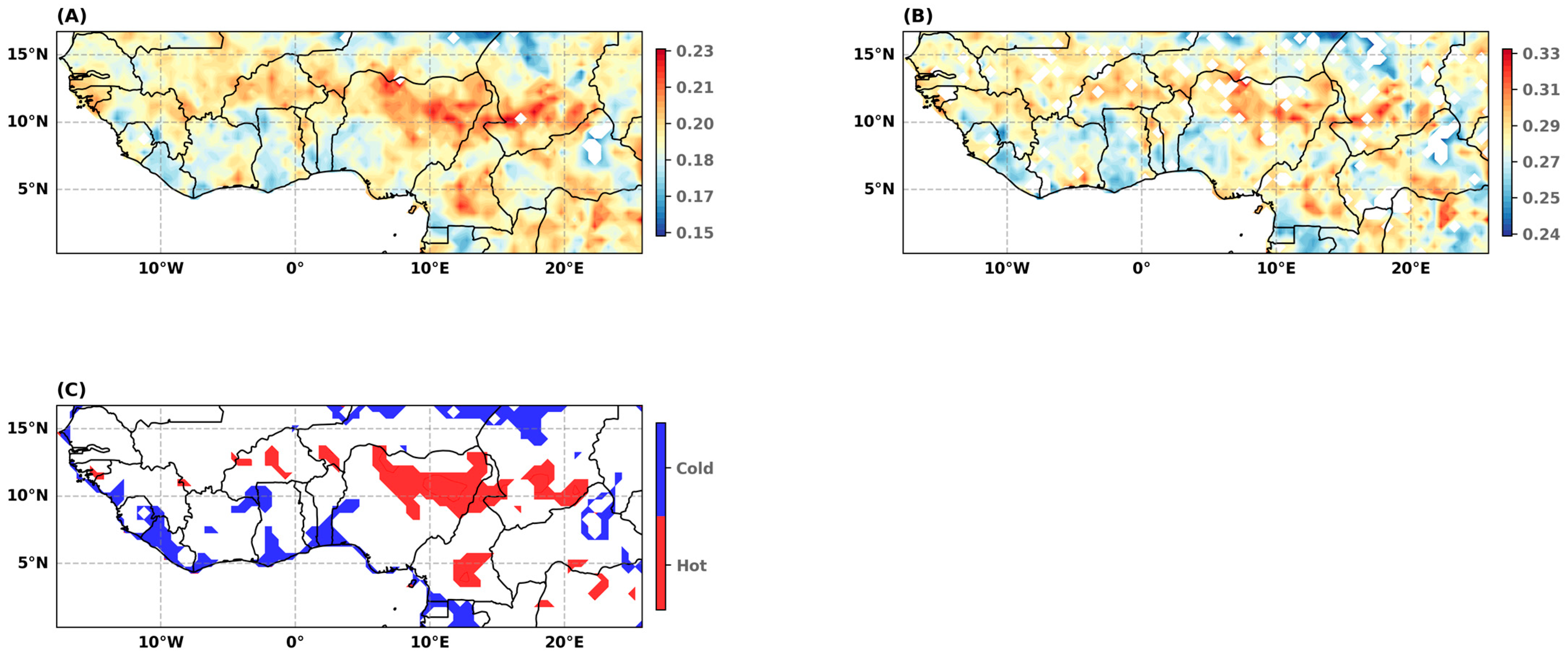
The spatial distribution of the DHIA (Figure 7A–C) shows that the area with the highest drought hazard index/DHI is located in northern Nigeria. This area forms a large cluster (hot spot) of high values with ramifications in northern Cameroon and southern Chad (red areas in Figure 7C). The center of Burkina Faso and Cameroon also appear as high-risk areas. By contrast, the drought hazard is relatively low in the coastal area between Guinea and western Ghana, as well as in the Western part of Cote d’Ivoire and South Benin (blue areas). Results for the northernmost part of the study area should be taken with caution due to the poor quality of the data in these arid areas. The spatial pattern that emerges from Figure 7A,B is similar, meaning that results are robust to the number of drought categories used to calculate the DHIA.
4.2.3. Extreme Drought Hazard Index
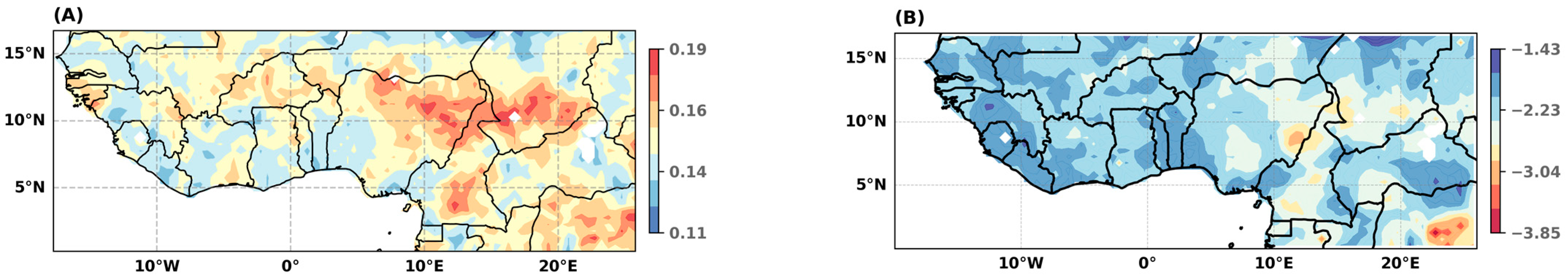
Considering that the estimated probability of non-exceedance of the extreme drought threshold is, on average, equal to 10.4%, we can restrict the number of drought categories used in the calculation of the DHI to droughts classified as severe to exceptional (categories 3 to 5 in Table 2). In that case, the DHIA map is shown in Figure 8A. The spatial distribution of extreme hazard is quite similar to that of the drought hazard shown in Figure 7B.
The centennial drought’s return level gives another picture of the extreme drought hazard. The centennial drought has a return period of 100 years and a return level equal to the first percentile of the distribution. Therefore, the 100-year return level is the amount of annual rainfall total that can be expected on average in one year out of 100. After standardization, the return level of the centennial drought can be considered as an extreme drought hazard index. It is equal to the DHIA calculated for one category of droughts only: those with a probability of occurrence less than or equal to 1%. In other words, lower intensity drought categories are given a zero weight in Equation (6). The map of the extreme hazard (Figure 8B) is quite different than that of the DHIA (Figure 7). The epicenter of the extreme hazard area moves towards the central eastern part of the region. The extreme drought hazard, measured as the severity of the 100-year drought, is higher in the eastern part of the region, with a hot spot spanning three countries, Nigeria, Chad, and Cameroon.
Table 3 confirms that the GNG mixture model is more efficient in identifying centennial droughts than the standard approach based on the SPI. The number of dry spells with an annual rainfall total less than or equal to that of the 100-year drought differs greatly depending on whether it is calculated using the GNG or the SPI distribution. According to the SPI approach, 12.45% of locations did not experience a rainfall episode equal to or below the 100-year drought level, while 23.45% of locations experienced more than two drought years below the 100-year level in the period 1901–2020. The results are more consistent when using the GNG distribution: only six of 2298 locations did not experience a drought spell below the 100-year drought level, and only 4.1% of locations experienced more than two drought episodes below the 100-year level.
5. Conclusions
The objective of the paper is to propose a method to estimate drought hazard over a large and climatically heterogeneous region. The accurate assessment of drought hazard and hazard prone locations provides important information to guide economic operators in their investment choices, as well as insurers and governments in the design of drought-risk management tools and risk-coping strategies. A critical stage in drought hazard assessment is the classification of drought events according to their intensity. We have shown that the commonly used method for calculating the DHI, which is based on the standardized precipitation index, does not allow for the assessment of region-specific hazards. In the SPI approach, differences in the level of the DHI from one precipitation distribution to another are statistical artifacts.
The method we propose in this paper is based on the estimation of an extreme value mixture model, which offers at least two advantages over the SPI approach. First, our GNG mixture model fits the data well, indeed, better than the standardized precipitation index. In particular, the GNG model performs better to identify extreme precipitation in the left tail of the distribution. Thus, the model can be used for predictive purposes to estimate the occurrence probability or return level of rare events. Second, the extreme value mixture model provides an objective estimation of the extreme drought threshold. Therefore, the quantile function of the model can be used (i) to measure the drought intensity at a selected set of return periods, (ii) to calculate the drought hazard index, and (iii) to calculate an extreme DHI when restricting the calculation to rare drought events. By construction, the DHI value varies according to the characteristics of the left tail of each precipitation distribution.
Another advantage of the proposed method is its operational aspect. Drought thresholds can be easily estimated and the estimation accuracy tested. As they are measured in the same unit as the rainfall data (mm per year in our case), a rainfall deficit can be readily classified and appropriate responses quickly triggered.
The application conducted on an indicator of meteorological drought, the annual precipitation total, and about 2300 gridded time series in the West and Central parts of sub-Saharan Africa show that the main hot spots of high DHI values are located in the northern part of Nigeria, the southern part of Chad, and the central part of Cameroon, respectively. It is important to keep in mind that those areas where the drought hazard is the greatest are not necessarily those where the risk is the greatest. The risk associated with a hazard depends on the vulnerability of the socioeconomic activities and natural systems exposed to the hazard.
This analysis should be considered as exploratory. Its scope could be extended to a larger geographic area and to other precipitation indexes such as the cumulative precipitation during the plant growth period or the SPEI. The results obtained for the right tail of the distribution, modeled with a generalized Pareto distribution, could also be exploited to define a heavy rainfall threshold and estimate heavy rainfall hazards. In addition, a number of limitations should be addressed in the future research. In a drought hazard assessment, the rainfall distribution assumptions made are crucial, and the relevancy of the drought hazard estimates depends on the goodness-of-fit of the assumed distribution. We have shown that the GPD–Normal–GPD mixture model fits the data well, but a still better-fitting model can always be looked for. The main challenge for the future research relates to the non-stationarity of the data in relation to climate change. The tests have shown that this should not be a major problem for the period and region studied, although a break in the mean level of precipitation in the late 1960s cannot be ruled out for some areas. In this respect, Heidari, H. et al. [52] have shown that a mixture model with time-varying parameters estimated on a moving window of a nonstationary time series can address shifts in precipitation distribution and performs better under changing climate conditions than classic families of distribution. These encouraging results obtained for a gamma–GPD mixture model plead for further research in this direction.
Author Contributions
Conceptualization, C.A.B. and M.-E.D.; methodology, all authors; software, A.S. and C.A.B.; validation, all authors; formal analysis, A.S. and C.A.B.; investigation, all authors; resources, C.A.B.; data curation, A.S.; writing—original draft preparation, C.A.B.; writing—review and editing, all authors; visualization, A.S.; supervision, C.A.B. and M.-E.D.; project administration, C.A.B. and M.-E.D.; funding acquisition, C.A.B. All authors have read and agreed to the published version of the manuscript.
Funding
This research was funded by the Agence Nationale de la Recherche of the French government though the IDEX-ISITE initiative (16-IDEX-0001 CAP 20-25) and the LABEX IDGM+ (ANR-10-LABX-14-01), within the program “Investissements d’Avenir”.
Data Availability Statement
The data were extracted from the revised January 2021 version of the dataset referred to as CRU TS4.05. They are available at: https://crudata.uea.ac.uk/cru/data/hrg/cru_ts_4.05/ accessed on 28 March 2022. The main software used is the Evmix R package developed by [45]: https://cran.r-project.org/web/packages/evmix/index.html accessed on 28 March 2022.
Acknowledgments
The authors are grateful to the members of the project “Modélisation des aléas climatiques en Afrique de l’Ouest”, specifically to Nourddine Azzaoui and Arnaud Guillin (LMBP, University of Clermont Auvergne) for insightful discussions on methodological aspects, and to Olivier Santoni (CERDI, University of Clermont Auvergne) for assistance in data collection.
Conflicts of Interest
The authors declare no conflict of interest. The funders had no role in the design of the study; in the collection, analyses, or interpretation of data; in the writing of the manuscript; or in the decision to publish the results.
Appendix A
Return level plot: simulation results.
Figure A1.
Simulation results. Each of the return plots illustrates the impact of changing one parameter of the left tail GDP, all else being equal. (A) An increase in the left threshold (location parameter μL) shifts the whole distribution upward. (B) A change in the shape parameter (ξl) affects the curvature of the plot: the level of extreme precipitation decreases rapidly to the bound for a large negative value of ξl; it decreases slowly for a positive value of ξl. (C) An increase in the scale parameter σl affects the slope of the distribution: the level of rare extreme precipitation decreases more than that of more frequent events.

Appendix B
Uncertainty and sensitivity analysis
Uncertainty in the value of the model’s parameters, θ, results in uncertainty in q = q(θ), the model’s output. q is the vector of the predicted values of precipitation, and θ is the vector of the GNG parameters. To implement the uncertainty and sensitivity analysis, we take advantage of our large sample of estimation results. The mixture model was estimated on 2298 precipitation series, generating 2298 vectors θ of parameter values and 2298 × n output. Therefore, we use the empirical distribution of the parameters instead of using sampling-based methods, which would imply assigning a hypothetical distribution to θ elements. This approach allows us to circumvent the issue of non-independent parameters. As some of the input variables are correlated, parameters cannot be drawn independently.
To assess the uncertainty in the model’s results, given the uncertainty in θ, we examine the distribution of a selected number of precipitation quantiles using boxplots. To assess the importance of each individual element of θ with respect to the uncertainty in q(θ), we draw on regression analysis [55,56].
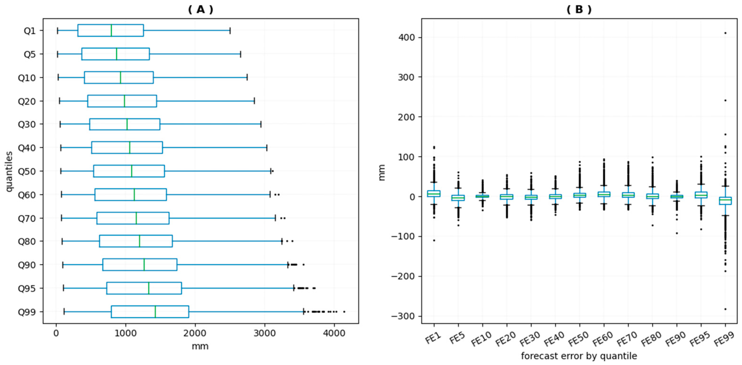
Figure A2(A) shows that the uncertainty in the model’s predictions is higher for high levels of precipitation: the whisker tends to be longer for the high quantiles, especially for the 99th quantile, and the number of outliers above the upper staple increases from the median to the 99th quantile. This result partly reflects the greater dispersion of extreme precipitation levels observed in the empirical data. To eliminate this source of bias in interpretation, we estimate the uncertainty in the forecast errors. The forecast error for the quantile i of the distribution k is measured in relative terms and given by: with the empirical quantile i of the precipitation distribution k, θk the vector of the parameters of the distribution k, and qi(θk) the theoretical quantile i of the distribution k, i = 1%, 5%, 10%, …, 90%, 95%, 99%, and k = 1 to 2298. Figure A2(B)shows the uncertainty in the forecast errors with respect to the value of the model’s parameters by precipitation quantile. Uncertainty tends to be higher in extreme quantiles, with more outliers in the lowest and highest quantiles.
Figure A2.
Representation of uncertainty in the model’s results. (A) Uncertainty in the predicted precipitation values by quantile. (B) Uncertainty in the forecast error by precipitation quantile.
Figure A2.
Representation of uncertainty in the model’s results. (A) Uncertainty in the predicted precipitation values by quantile. (B) Uncertainty in the forecast error by precipitation quantile.

For purposes of the sensitivity analysis, we compute the partial correlation coefficients (PCC) between q, an arbitrary element of q, and the element j of vector θ. The PCC measures the strength of the relationship between the two variables with the effect of other parameters removed. Whatever the correlation degree between the GNG parameters, the PCC allows us to assess the importance of each element of θ, holding the other one constant. The PCC between q and is given by the correlation coefficient between and with:
and
Another approach to the sensitivity analysis consists of calculating the coefficients of partial determination (CPD). The CPD provide information on the fraction of uncertainty in q that is accounted for by θj. To account for the correlation between the parameters of the mixture model, we compute the CPD as the difference between the R2 of the full model and the R2 of the reduced model given by Equation (A2). The full model includes all elements of θ so that the associated coefficient of determination is close to 1. The CPD represents the fraction of the variance of q explained by θj, controlling for all other model’s variables.
Equations (A1) and (A2) are estimated for a select number of precipitation quantiles qi with i = 1 p, 5 p, 10 p, …, 90 p, 95 p, 99 p. The absolute value of PCCs are provided in Figure A3(A). As expected, the figure shows that precipitation values in the lowest and highest quantiles are strongly correlated with the left and right GPD parameters, respectively. The most important parameters in the extremes of the distribution are, by importance order, location, scale, and shape parameters of the corresponding GPD. In the center of the distribution, the most important parameter is the Gaussian mean. We note that the PCCs are symmetrically distributed around the median axis. For instance, the PCC between ur and the qi is equal to the PCC between ul and q1−i, with qi the i-th quantile. We note also that precipitation values from the 10th to the 90th quantiles are correlated, but in a decreasing (increasing) way, with the location parameters of the left (right) GPD and all other parameters held constant.
Figure A3.
Sensitivity analysis. (A) Partial correlation coefficients in absolute value. (B) Coefficients of partial determination.
Figure A3.
Sensitivity analysis. (A) Partial correlation coefficients in absolute value. (B) Coefficients of partial determination.

These results are confirmed by the coefficients of partial determination. Figure A3(B) shows that the GPD’s parameters contribute most to the variance of the mixture’s output in the lowest and highest quantiles of precipitation, the location parameters being the most influential parameters. Precipitation levels in the center of the distribution are more sensitive to the location parameter of the Gaussian. Figure A3(B) also shows the importance of the shape and scale parameters of the two GPD in explaining the variance of extreme quantiles. We note that the sum of the CPD is much lower than 1, indicating the importance of interactions between the GNG’s parameters.
References
- Carrão, H.; Naumann, G.; Barbosa, P. Mapping Global Patterns of Drought Risk: An Empirical Framework Based on Sub-National Estimates of Hazard, Exposure and Vulnerability. Glob. Environ. Change 2016, 39, 108–124. [Google Scholar] [CrossRef]
- Vogt, J.V.; Naumann, G.; Masante, D.; Spinoni, J.; Cammalleri, C.; Erian, W.; Pischke, F.; Pulwarty, R.; Barbosa, P. Drought Risk Assessment and Management—A Conceptual Framework; EUR 29464 EN; Publications Office of the European Union: Luxembourg, 2018. [Google Scholar] [CrossRef]
- Hagenlocher, M.; Meza, I.; Anderson, C.C.; Min, A.; Renaud, F.G.; Walz, Y.; Siebert, S.; Sebesvari, Z. Drought vulnerability and risk assessments: State of the art, persistent gaps, and research agenda. Environ. Res. Lett. 2019, 14, 083002. [Google Scholar] [CrossRef]
- Mens, M.J.P.; van Rhee, G.; Schasfoort, F.; Kielen, N. Integrated drought risk assessment to support adaptive policymaking in the Netherlands. Nat. Hazards Earth Syst. Sci. 2022, 22, 1763–1776. [Google Scholar] [CrossRef]
- Ó Gráda, C. Making Famine History. J. Econ. Lit. 2007, 45, 5–38. [Google Scholar] [CrossRef]
- Wilhite, D.A.; Sivakumar, M.V.K.; Pulwarty, R. Managing Drought Risk in a Changing Climate: The Role of National Drought Policy. Weather Clim. Extrem. 2014, 3, 4–13. [Google Scholar] [CrossRef] [Green Version]
- Tadesse, T. Strategic Framework for Drought Risk Management and Enhancing Resilience in Africa; White Paper; UNCCD: Bonn, Germany, 2018. [Google Scholar]
- Hayes, M.J.; Wilhelmi, O.V.; Knutson, C.L. Reducing Drought Risk: Bridging Theory and Practice. Nat. Hazards Rev. 2004, 5, 106–113. [Google Scholar] [CrossRef]
- Vicente-Serrano, S.M.; Beguería, S.; Gimeno, L.; Eklundh, L.; Giuliani, G.; Weston, D.; El Kenawy, A.; López-Moreno, J.I.; Nieto, R.; Ayenew, T.; et al. Challenges for drought mitigation in Africa: The potential use of geospatial data and drought information systems. Appl. Geogr. 2012, 34, 471–486. [Google Scholar] [CrossRef] [Green Version]
- World Bank. Assessing Drought Hazard and Risk: Principles and Implementation Guidance; World Bank: Washington, DC, USA, 2019; Available online: http://documents.worldbank.org/curated/en/989851589954985863/Assessing-Drought-Hazard-and-Risk-Principles-and-Implementation-Guidance (accessed on 21 June 2022).
- IPCC. Managing the Risks of Extreme Events and Disasters to Advance Climate Change Adaptation; Field, C.B., Barros, V., Stocker, T.F., Qin, D., Dokken, D.J., Ebi, K.L., Mastrandrea, M.D., Mach, K.J., Plattner, G.-K., Allen, S.K., et al., Eds.; A Special Report of Working Groups I and II of the Intergovernmental Panel on Climate Change; Cambridge University Press: Cambridge, UK; New York, NY, USA, 2012; Available online: https://www.ipcc.ch/site/assets/uploads/2018/03/SREX_Full_Report-1.pdf (accessed on 8 January 2020).
- Rajsekhar, D.; Singh, V.P.; Mishra, A.K. Integrated Drought Causality, Hazard, and Vulnerability Assessment for Future Socioeconomic Scenarios: An Information Theory Perspective. J. Geophys. Res. Atmos. 2015, 120, 6346–6378. [Google Scholar] [CrossRef]
- Dracup, J.A.; Lee, K.S.; Paulson, E.G. On the definition of droughts. Water Resour. Res. 1980, 16, 297–302. [Google Scholar] [CrossRef]
- Wilhite, D.A.; Glantz, M.H. Understanding: The Drought Phenomenon: The Role of Definitions. Water Int. 1985, 10, 111–120. [Google Scholar] [CrossRef] [Green Version]
- Mishra, A.K.; Singh, V.P. A review of drought concepts. J. Hydrol. 2010, 391, 202–216. [Google Scholar] [CrossRef]
- WMO; GWP. Handbook of Drought Indicators and Indices; Svoboda, M., Fuchs, B.A., Eds.; Integrated Drought Management Tools and Guidelines Series 2; Integrated Drought Management Programme (IDMP): Geneva, Switzerland, 2016. [Google Scholar]
- Wilhite, D.A. Drought as a natural hazard: Concepts and definitions. In Drought: A Global Assessment; Wilhite, D.A., Ed.; Routledge Publishers: London, UK, 2000; Volume I, Chapter 1; pp. 3–18. [Google Scholar]
- McKee, T.; Doesken, N.J.; Kleist, J. The Relationship of Drought Frequency and Duration to Time Scales. In Proceedings of the Eighth Conference on Applied Climatology, Anaheim, CA, USA, 17–22 January 1993. [Google Scholar]
- Vicente-Serrano, S.M.; Beguería, S.; López-Moreno, J.L. A Multiscalar Drought Index Sensitive to Global Warming: The Standardized Precipitation Evapotranspiration Index. J. Clim. 2010, 23, 1696–1718. [Google Scholar] [CrossRef] [Green Version]
- Palmer, W.C. Meteorological Drought; Research Paper, No. 45; US Weather Bureau: Washington, DC, USA, 1965; Available online: https://www.droughtmanagement.info/literature/USWB_Meteorological_Drought_1965.pdf (accessed on 11 August 2023).
- Guttman, N.B. Accepting the Standardized Precipitation Index: A Calculation Algorithm1. JAWRA J. Am. Water Resour. Assoc. 1999, 35, 311–322. [Google Scholar] [CrossRef]
- Edwards, D.; McKee, T. Characteristics of 20th Century Drought in The United States at Multiple Time Scales; Climatology Report No 97-2; Department of Atmospheric Science, Colorado State University: Fort Collins, CL, USA, 1997; Volume 97-2. [Google Scholar]
- Shahid, S.; Behrawan, H. Drought Risk Assessment in the Western Part of Bangladesh. Nat. Hazards 2008, 46, 391–413. [Google Scholar] [CrossRef]
- He, B.; Lü, A.; Wu, J.; Zhao, L. Drought hazard assessment and spatial characteristics analysis in China. J. Geogr. Sci. 2011, 21, 235–249. [Google Scholar] [CrossRef]
- Svoboda, M.D.; LeComte, D.; Hayes, M.; Heim, R.; Gleason, K.; Angel, J.; Rippey, B.; Tinker, R.; Palecki, M.; Stooksbury, D.; et al. The drought monitor. Bull. Am. Meteorol. Soc. 2002, 83, 1181–1190. [Google Scholar] [CrossRef] [Green Version]
- Şen, Z.; Almazroui, M. Actual Precipitation Index (API) for Drought classification. Earth Syst. Env. 2021, 5, 59–70. [Google Scholar] [CrossRef]
- Carrão, H.; Singleton, A.; Naumann, G.; Barbosa, P.; Vogt, J. An optimized system for the classification of meteorological drought intensity with applications in frequency analysis. J. Appl. Meteorol. Climatol. 2014, 53, 1943–1960. [Google Scholar] [CrossRef] [Green Version]
- Pickands, J. Statistical inference using extreme order statistics. Ann. Stat. 1975, 3, 119–131. [Google Scholar] [CrossRef]
- Balkema, A.A.; de Haan, L. Residual Life Time at Great Age. Ann. Probab. 1974, 2, 792–804. [Google Scholar] [CrossRef]
- Leadbetter, M.R. On a basis for ‘Peaks over Threshold’ modeling. Stat. Probab. Lett. 1991, 12, 357–362. [Google Scholar] [CrossRef]
- Coles, S. An Introduction to Statistical Modeling of Extreme Values; Springer: London, UK, 2001. [Google Scholar] [CrossRef]
- Gharib, A.; Davies, E.G.R.; Goss, G.G.; Faramarzi, M. Assessment of the Combined Effects of Threshold Selection and Parameter Estimation of Generalized Pareto Distribution with Applications to Flood Frequency Analysis. Water 2017, 9, 692. [Google Scholar] [CrossRef] [Green Version]
- Pan, X.; Rahman, A.; Haddad, K.; Ourda, T.B.M.J. Peaks-over-threshold model in flood frequency analysis: A scoping review. Stoch. Environ. Res. Risk Assess. 2022, 36, 2419–2435. [Google Scholar] [CrossRef]
- Kim, J.E.; Yoo, J.; Chung, G.H.; Kim, T.-W. Hydrologic Risk Assessment of Future Extreme Drought in South Korea Using Bivariate Frequency Analysis. Water 2019, 11, 2052. [Google Scholar] [CrossRef] [Green Version]
- Burke, E.J.; Perry, R.H.J.; Brown, S.J. An extreme value analysis of UK drought and projections of change in the future. J. Hydrol. 2010, 388, 131–143. [Google Scholar] [CrossRef]
- Scarrott, C.; MacDonald, A. A review of extreme value threshold estimation and uncertainty quantification. REVSTAT-Stat. J. 2012, 10, 33–59. [Google Scholar] [CrossRef]
- Langousis, A.; Mamalakis, A.; Puliga, M.; Deidda, R. Threshold detection for the generalized Pareto distribution: Review of representative methods and application to the NOAA NCDC daily rainfall database. Water Resour. Res. 2016, 52, 2659–2681. [Google Scholar] [CrossRef] [Green Version]
- Harris, I.; Jones, P.D.; Osborn, T.J.; Lister, D.H. Updated high-resolution grids of monthly climatic observations—The CRU TS3.10 Dataset. Int. J. Climatol. 2014, 34, 623–642. [Google Scholar] [CrossRef] [Green Version]
- Solari, S.; Losada, M.A. A unified statistical model for hydrological variables including the selection of threshold for the peak over threshold method. Water Resour. Res. 2012, 48, 1–15. [Google Scholar] [CrossRef]
- MacDonald, A.; Scarrott, C.J.; Lee, D.; Darlow, B.; Reale, M.; Russell, G. A flexible extreme value mixture model. Comput. Stat. Data Anal. 2011, 55, 2137–2157. [Google Scholar] [CrossRef]
- Behrens, C.N.; Lopes, H.F.; Gamerman, D. Bayesian analysis of extreme events with threshold estimation. Stat. Model. 2004, 4, 227–244. [Google Scholar] [CrossRef] [Green Version]
- Mendes, B.; Lopes, H.F. Data driven estimates for mixtures. Comput. Stat. Data Anal. 2004, 47, 583–598. [Google Scholar] [CrossRef]
- Zhao, X.; Scarrott, C.J.; Reale, M.; Oxley, L. Extreme value modelling for forecasting the market crisis. Appl. Financ. Econ. 2010, 20, 63–72. [Google Scholar] [CrossRef]
- Tukey, J.W. A Survey of Sampling from Contaminated Distributions. In Contribution to Probability and Statistics, Essays in Honor of Herald Hotelling; Olkin, I., Goraye, S.G., Hoeffding, W., Madow, W.G., Mann, H.B., Eds.; Stanford University Press: Stanford, CA, USA, 1960. [Google Scholar]
- Hu, Y.; Scarrott, C. Evmix: Extreme Value Mixture Modelling, Threshold Estimation and Boundary Corrected Kernel Density Estimation. R package Version 2.10. J. Stat. Softw. 2018, 84, 1–27. [Google Scholar] [CrossRef] [Green Version]
- Hubert, P.; Carbonnel, J.P.; Chaouche, A. Segmentation des séries hydrométéorologiques—Application à des séries de précipitations et de débits de l’afrique de l’ouest. J. Hydrol. 1989, 110, 349–367. [Google Scholar] [CrossRef]
- Ali, A.; Lebel, T. The Sahelian standardized rainfall index revisited. Int. J. Climatol. 2009, 29, 1705–1714. [Google Scholar] [CrossRef]
- Panthou, G.; Vischel, T.; Lebel, T. Recent trends in the regime of extreme rainfall in the Central Sahel. Int. J. Climatology 2014, 34, 3998–4006. [Google Scholar] [CrossRef]
- Descroix, L.; Diongue Niang, A.; Panthou, G.; Bodian, A.; Sane, Y.; Dacosta, H.; Malam Abdou, M.; Vandervaere, J.P.; Quantin, G. Évolution récente de la pluviométrie en Afrique de l’ouest à travers deux régions: La Sénégambie et le Bassin du Niger Moyen. Climatologie 2015, 12, 25–43. [Google Scholar] [CrossRef] [Green Version]
- Biasutti, M. Rainfall trends in the African Sahel: Characteristics, processes, and causes. WIREs Clim. Change 2019, 10, e591. [Google Scholar] [CrossRef]
- Pettitt, A.N. A Non-Parametric Approach to the Change-Point Problem. J. R. Stat. Society. Ser. C Appl. Stat. 1979, 28, 126–135. [Google Scholar] [CrossRef]
- Heidari, H.; Arabi, M.; Ghanbari, M.; Warziniack, T. A probabilistic approach for characterization of sub-annual socioeconomic drought intensity-duration-frequency (IDF) relationships in a changing environment. Water 2020, 12, 1522. [Google Scholar] [CrossRef]
- Diebold, F.X.; Mariano, R. Comparing Predictive Accuracy. J. Bus. Econ. Stat. 2002, 20, 134–144. [Google Scholar] [CrossRef]
- Harvey, D.; Leybourne, S.J.; Newbold, N. Tests for Forecast Encompassing. J. Bus. Econ. Stat. 1998, 16, 254–259. [Google Scholar] [CrossRef]
- Helton, J.C.; Bean, J.E.; Economy, K.; Garner, J.W.; MacKinnon, R.J.; Miller, J.; Schreiber, J.D.; Vaughn, P. Uncertainty and sensitivity analysis for two-phase flow in the vicinity of the repository in the 1996 performance assessment for the Waste Isolation Pilot Plant: Undisturbed conditions. Reliab. Eng. Syst. Saf. 2000, 69, 227–261. [Google Scholar] [CrossRef]
- Helton, J.C.; Johnson, J.D.; Sallaberry, C.J.; Storli, C.B. Survey of sampling-based methods for uncertainty and sensitivity analysis. Reliab. Eng. Syst. Saf. 2006, 91, 1175–1209. [Google Scholar] [CrossRef] [Green Version]
Figure 1.
Average annual rainfall over the period 1901–2016 (mm).

Figure 2.
Results of simulations: probability density of a GPD–Normal–GPD mixture model (orange) and of Gaussian distribution (blue). The two distributions have the same mean.
Figure 2.
Results of simulations: probability density of a GPD–Normal–GPD mixture model (orange) and of Gaussian distribution (blue). The two distributions have the same mean.

Figure 3.
Stationarity and independence test results. (A) ADF unit root test, with intercept and trend in the test equation. Red cells: the test does not reject the null hypothesis of unit root. (B) Pettit test: red cells: rejection of the no change point null hypothesis. (C) Autocorrelation test on the POT series: Box-Pierce/Ljung-Box Q-statistics for serial correlation up to the order 1. Red cells: rejection of no serial correlation at lag 1.

Figure 4.
Goodness-of-fit test results. (A) Kolmogorov–Smirnov test; Red cells: bootstrap p-value < 0.05, the GNG does not fit the data. (B) Diebolt and Mariano test; Loss function: absolute error. H0: Both forecasts have the same accuracy. Green cells: H0 is rejected against the alternative hypothesis (H1a) that the GNG is more accurate than the gamma model. Red cells: H0 is rejected against the alternative hypothesis (H1b) that the GNG is less accurate than the gamma model. Yellow cells: H0 is not rejected against both alternatives H1a and H1b.

Figure 5.
GNG parameters. (A) Location parameter (ul) after standardization; (B) probability of being below the left threshold (ϕul); (C) scale parameter (σl); (D) shape parameter (ξl).
Figure 5.
GNG parameters. (A) Location parameter (ul) after standardization; (B) probability of being below the left threshold (ϕul); (C) scale parameter (σl); (D) shape parameter (ξl).

Figure 6.
DHI calculated from Equation (5) using the SPI (A) and the GNG (B).

Figure 7.
Alternative drought hazard index (DHIA) mapping. (A) DHIA calculated using Equation (6) and three drought categories, from moderate to extreme, given in Table 1. (B) DHIA calculated using Equation (6) and four drought categories, from moderate to exceptional, given in Table 2. (C). Hot and cold spots of the DHIA given in Figure 8A.

Figure 8.
Extreme drought hazard index. (A) DHIA calculated for severe to exceptional droughts. (B) standardized value of the 100-year drought return level.
Figure 8.
Extreme drought hazard index. (A) DHIA calculated for severe to exceptional droughts. (B) standardized value of the 100-year drought return level.


Table 1.
Drought categories and thresholds of [18].
Table 1.
Drought categories and thresholds of [18].
| Drought Category | Weight Wi | Threshold Values for the SPI | Thresholds in Percentiles | Prob. of Occurrence (ϕi) | Empirical Frequency (fi): SPI | Empirical Frequency (fi): GNG |
|---|---|---|---|---|---|---|
| 1. Mild drought | 0 | 0.341 | 0.354 | 0.356 | ||
| 2. Moderate drought | 1 | [6.68%; 15.87%] | 0.92 | 0.079 | 0.096 | |
| 3. Severe drought | 2 | 0.04 | 0.040 | 0.041 | ||
| 4. Extreme drought | 3 | ≤−2 | 0.0227 | 0.029 | 0.0227 | |
| DHI (Equation (5)) | 0.24 | 0.243 | 0.246 |
Table 2.
Probability of occurrence and empirical frequency of droughts.
| Drought Category (USDA) | Percentiles | Theoretical Prob. of Occurrence (ϕi) | Empirical Frequency: GNG (fi) |
|---|---|---|---|
| 1. Abnormally dry | 10% | 0.096 | |
| 2. Moderate drought | 10% | 0.099 | |
| 3. Severe drought | 5% | 0.053 | |
| 4. Extreme drought | 3% | 0.027 | |
| 5. Exceptional drought | 2% | 0.021 | |
| Total | 30% | 0.295 |
Note(s): the empirical frequency is the mean frequency calculated over the whole sample, which includes 2981 locations and 263,754 annual rainfall observations.
Table 3.
Frequency of 100-year drought episodes in the period 1901–2020, for all grid cells.
| SPI | GNG | |||
|---|---|---|---|---|
| Value | Count | Percent | Count | Percent |
| 0 | 286 | 12.45 | 6 | 0.26 |
| 1 | 758 | 32.99 | 1406 | 61.18 |
| 2 | 715 | 31.11 | 791 | 34.42 |
| 3 | 424 | 18.45 | 89 | 3.87 |
| 4 | 95 | 4.13 | 6 | 0.26 |
| 5 | 19 | 0.83 | 0 | 0 |
| 6 | 1 | 0.04 | 0 | 0 |
| Total | 2298 | 100 | 2298 | 100 |
Disclaimer/Publisher’s Note: The statements, opinions and data contained in all publications are solely those of the individual author(s) and contributor(s) and not of MDPI and/or the editor(s). MDPI and/or the editor(s) disclaim responsibility for any injury to people or property resulting from any ideas, methods, instructions or products referred to in the content. |
© 2023 by the authors. Licensee MDPI, Basel, Switzerland. This article is an open access article distributed under the terms and conditions of the Creative Commons Attribution (CC BY) license (https://creativecommons.org/licenses/by/4.0/).
Share and Cite
MDPI and ACS Style
Araujo Bonjean, C.; Sy, A.; Dury, M.-E. Spatially Consistent Drought Hazard Modeling Approach Applied to West Africa. Water 2023, 15, 2935. https://doi.org/10.3390/w15162935
AMA Style
Araujo Bonjean C, Sy A, Dury M-E. Spatially Consistent Drought Hazard Modeling Approach Applied to West Africa. Water. 2023; 15(16):2935. https://doi.org/10.3390/w15162935
Chicago/Turabian StyleAraujo Bonjean, Catherine, Abdoulaye Sy, and Marie-Eliette Dury. 2023. "Spatially Consistent Drought Hazard Modeling Approach Applied to West Africa" Water 15, no. 16: 2935. https://doi.org/10.3390/w15162935
Note that from the first issue of 2016, this journal uses article numbers instead of page numbers. See further details here.