Article

Sediment Yield and Reservoir Sedimentation in Highly Dynamic Watersheds: The Case of Koga Reservoir, Ethiopia

1
Australian River Institute and School of Engineering, Griffith University, Nathan, QLD 4111, Australia
2
CERIS, Instituto Superior Técnico, Universidade de Lisboa, 1649-004 Lisbon, Portugal
3
College of Architecture and Civil Engineering, Addis Ababa Science and Technology University, Addis Ababa P.O. Box 16417, Ethiopia
4
State Climate Office of North Carolina, North Carolina State University, Raleigh, NC 27695, USA
5
Department of Biological and Agricultural Engineering, North Carolina State University, Raleigh, NC 27695, USA
6
Key Laboratory of Digital Earth Science, Aerospace Information Research Institute, Chinese Academy of Sciences, Beijing 100094, China
7
Ethiopian Ministry of Water Resources, Addis Ababa P.O. Box 5744, Ethiopia
8
Institute of Environment and Sustainable Development in Agriculture (IEDA), Chinese Academy of Agricultural Sciences (CAAS), Beijing 100081, China
9
College of Agricultural Engineering and Technology, Sher-e-Kashmir University of Agricultural Sciences and Technology of Kashmir, Shalimar Campus, Srinagar 190025, India
10
Ethiopian Institute of Water Resources, Addis Ababa University, Addis Ababa P.O. Box 150461, Ethiopia
11
Blackland Research & Extension Center, Texas A&M AgriLife Research, 720 East Blackland Rd, Temple, TX 76502, USA
12
Department of Earth and Environment, Institute of Environment, Florida International University, AHC-5-390, 11200 SW 8th Street, Miami, FL 33199, USA
*
Author to whom correspondence should be addressed.
Water 2021, 13(23), 3374; https://doi.org/10.3390/w13233374
Submission received: 24 October 2021 / Revised: 21 November 2021 / Accepted: 25 November 2021 / Published: 30 November 2021

Abstract

:
Soil erosion is exacerbated by unsustainable land-use activities and poor management practices, undermining reservoir storage capacity. To this effect, appropriate estimation of sediment would help to adopt sustainable land-use activities and best management practices that lead to efficient reservoir operations. This paper aims to investigate the spatial variability of sediment yield, amount of sediment delivery into the reservoir, and reservoir sedimentation in the Koga Reservoir using the Soil and Water Assessment Tool (SWAT). Sediment yield and the amount entered into the reservoir were also estimated using a rating curve, providing an alternative approach to spatially referenced SWAT generated suspended sediment load. SWAT was calibrated from 1991 to 2000 and validated from 2002 to 2007 using monthly observations. Model performance indicators showed acceptable values using Nash-Sutcliffe efficiency (NSE) correlation coefficient (R2), and percent bias (PBIAS) for flow (NSE = 0.75, R2 = 0.78, and PBIAS = 11.83%). There was also good agreement between measured and simulated sediment yields, with NSE, R2, and PBIAS validation values of 0.80, 0.79, and 6.4%, respectively. The measured rating curve and SWAT predictions showed comparable mean annual sediment values of 62,610.08 ton/yr and 58,012.87 ton/yr, respectively. This study provides an implication for the extent of management interventions required to meet sediment load targets to a receiving reservoir, providing a better understanding of catchment processes and responses to anthropogenic and natural stressors in mixed land use temperate climate catchments. Findings would benefit policymakers towards land and water management decisions and serve as a prototype for other catchments where management interventions may be implemented. Specifically, validating SWAT for the Koga Reservoir is a first step to support policymakers, who are faced with implementing land and water management decisions.

1. Introduction

The construction of dams to create an artificial impounded reservoir changes the stream’s natural conditions by reducing streamflow velocity. The reduction in flow velocity caused by damming results in silt deposition which, in turn, may lead to a rapid decrease in reservoir storage capacity. In practical studies, estimating sediment load for planning, designing, operating, and maintaining water resource structures follows lengthy and costly sediment transportation monitoring and sampling methods [1,2]. Predicting sediment yield and estimating temporal fluctuation is necessary for various tasks, including erosion control structure design [3], river morphological calculations, and assessment studies of various land use management strategies [4,5,6]. Quantifying soil erosion and sediment delivery that ultimately contributes to downstream reservoirs’ siltation is essential in highly erodible watersheds [7,8], particularly with storms of extreme rainfall intensity on agricultural land areas with distinctly unconsolidated soils [9]. Siltation creates a long-term socio-economic concern as sediments reach reservoirs, lowering reservoir water storage capacity [10].
Land degradation results in a high erosion process, causing elevated sediment loads and enhanced sediment deposition in reservoirs and channels within the river system. This, in turn, results in environmental and socio-economic losses by decreasing soil fertility, increasing the maintenance costs in hydropower plants and irrigation schemes. Sediment deposition along the river channel causes flooding in the surroundings [11]. Flow velocity and transport capacity diminish when streamflow enters natural lake reservoirs, providing a favorable environment for silt deposition. The quantity deposited in manmade lake reservoirs with outlets, on the other hand, is determined by the detention storage period, reservoir form, and operating methods.
In many regions of the world, global human-induced environmental changes are generating an excessive rise in geomorphic alterations and sediment flows [12]. Water erosion is one of the most significant land degradation problems, and poses a serious environmental threat [13]. Soil erosion resulting from overgrazing, poor land management, and deforestation is a significant problem in Ethiopia. Due to the undulating topography and steep and erosive rainfall enhanced under agricultural systems that limit protective soil cover, soil erosion is common in the Ethiopian highlands. High-intensity rainfall occurs in most parts of Ethiopia, where cultivated land has little surface cover to reduce the impact of high-intensity raindrops with high runoff potential. Furthermore, the basin’s dense livestock population and rapid population expansion strain land resources, resulting in forest clearance and overgrazing [14]. As part of the Ethiopian High Land Reclamation Studies, the Abbay River Basin integrated development Master plan for irrigation development, integrated watershed management, soil erosion status, and sediment yield calculations were carried out in the study region [15]. The Koga watershed is one of the watersheds plagued by significant soil erosion, according to BECEOM studies, with an estimated suspended sediment production of 4.1 t/ha/yr [15].
Reservoir sedimentation reduces storage capacity, impede the functionality of intake structures, and accelerates the abrasion of hydraulic machinery, which lowers efficiency causing higher maintenance costs. The loss of storage also impacts water availability and operation schedules [16]. Land use, climate, and various landscape characteristics such as elevation, slope, soil type, vegetation, and drainage conditions influence sediment supply in a watershed [17]. Soil erosion deposes sediment particles in the reservoir, thereby decreasing the storage capacity of reservoirs. The water level variation determines delta formation, which gradually reduces the reservoir’s usable capacity. Sediments reaching the dam and passing through spillway and ducts causes a distinct environmental impact.
Despite the awareness of sediment inflow issues to a reservoir from gross soil erosion estimates, limited studies have been carried out to determine spatiotemporal variability of sediment yield entering reservoirs [16], to evaluate offsite and on-site effects of soil erosion, to identify critical sub-watersheds contributing high sediment for planning, and implementation of sufficient land and water management interventions. Watershed management interventions that involve systems to manage and utilize land, water, and vegetation resources include soil and water conservation. Physical/engineering and agronomic or vegetative soil and water conservation methods are also widely employed [18]. Concerning reservoir management, implementation of sluicing density current and hyper-concentrated density current and holding clear and flushing turbid water is the primary sediment management technique for large reservoirs [19]. Sediment delivery in Ethiopia’s highlands is influenced by outflow, rainfall, land use, and land cover that changes seasonally [20]. Sediment rating curves are complicated as a result, and sediment budgets are seldom created [9]. Although many studies have been performed in small watersheds [4,6,17], much less is known about sediment dynamics in a medium-scale watershed [21], which triggers the importance of predicting long-term sediment yield on the size and life of the reservoir.
Reservoirs appear to accumulate sediments more rapidly than what was initially estimated. The leading possible cause could be an inaccurate representation of possible future changes in management practices [22]. Current knowledge of catchment conditions, soil erosion, and deposition could help to ensure the implementation of appropriate remedial measures. In this regard, assessing catchment conditions and estimating resulting changes in streamflow and sediment deposition into the Koga dam reservoir is a topic of discussion to policymakers. Unlike other studies in the basin, this research combines rating curve-based sediment yield predictions using sparse observation data in a time series and outputs of a daily time step semi-distributed hydrological model.
Understanding the hydrological connectivity between areas of sediment mobilization and the receiving reservoir is essential to assess the impacts of management practices on receiving environments [23,24]. However, quantifying the complex relationships between hydrological variables can be difficult without hydrological models [25], which are key tools to address a wide spectrum of water resource management issues. Distributed hydrological models with input parameters representing different land surface characteristics have been applied to assess anthropogenic impacts on runoff and changes in sediment dynamics [25]. These models can also identify sediment source areas and prioritize catchments and sub-catchments to make informed policy decisions regarding land use planning and future catchment management [26].
In this study, in addition to the rating curve method, a basin-scale distributed hydrological model, the Soil and Water Assessment Tool (SWAT; [27]), was used to estimate streamflow and sediment load in a medium-sized hillslope-dominated watershed. SWAT is computationally efficient at evaluating long-term impacts, accounting for spatial heterogeneity within catchments, and assessing non-point source pollution and soil erosion controls [27,28,29].
This paper aims to determine major sediment sources in the Ethiopian highlands by quantifying geographic variability in sediment output from a medium-sized watershed and assessing future environmental implications by implementing methods to estimate the total amount of sediment yield into the reservoir and reservoir sedimentation rate. The specific objective of the study was to (1) assess the spatial variability of sediment yield and identify vulnerable sub-watersheds for erosion and sediment yield, (2) quantify the amount of sediment inflow into the reservoir, and (3) predict the total amount of sediment in the reservoir.

2. Materials and Methods

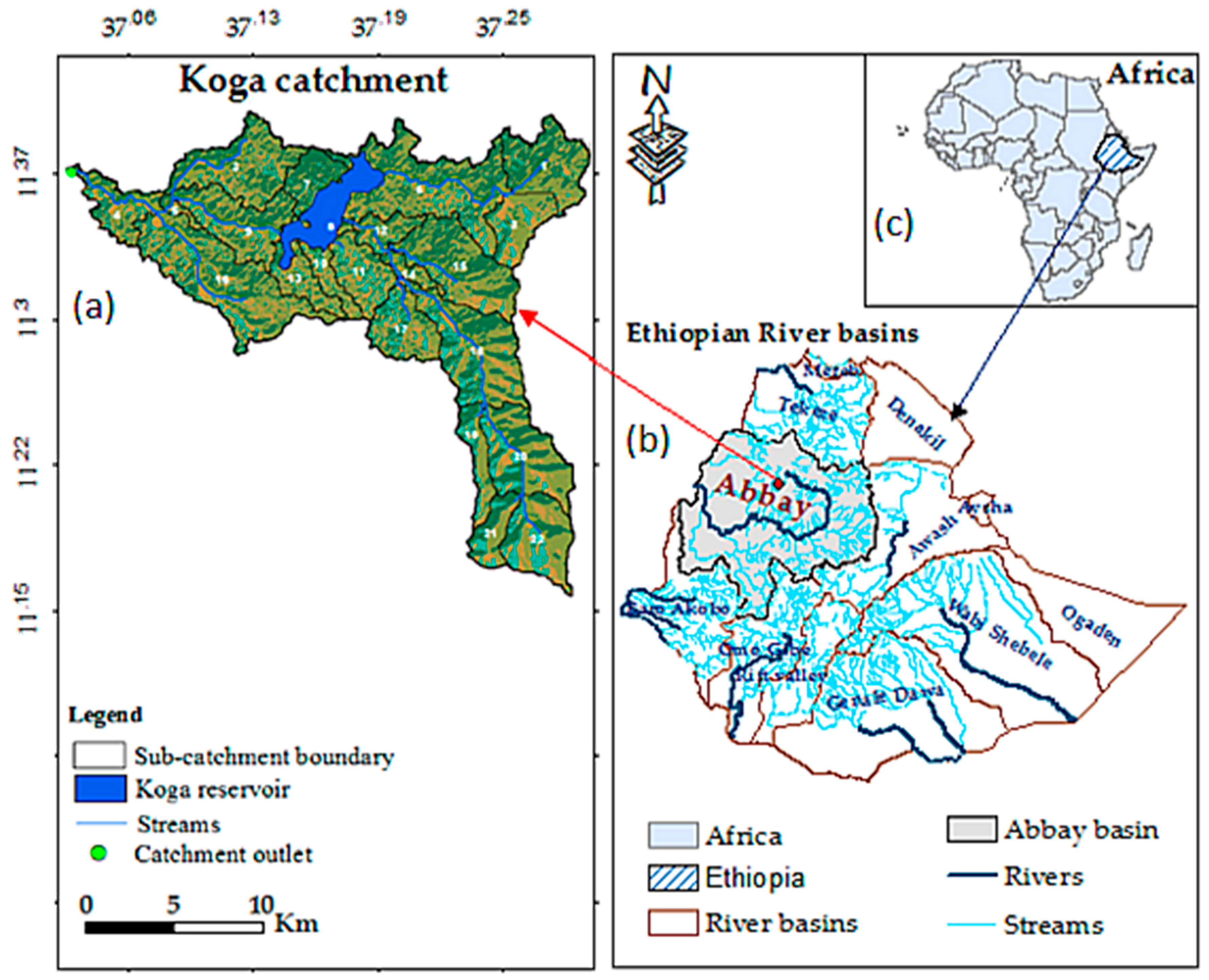
2.1. Description of Koga Reservoir

The Koga River is located in Northwest Ethiopia (Figure 1) and rises at around 3200 m above sea level. It feeds into the Gilgel Abay River (primary inflow source of the Blue Nile). At the Merawi gauging station, the Koga River drains a 287 km2 watershed. The Koga Reservoir consists of a 21.5 m high earth dam, and a 1860 m long, 18.50 m high, 1106 m wide saddle dam about 6 km northeast. The reservoir’s storage capacity at the full supply level (FSL, 2015.25 m above sea level) is 83.1 Mm3 or 71% of the mean annual runoff. At FSL, 18.59 km2 of land is underwater. The reservoir supplies about 7000 hectares of dry season irrigation and 5600 ha of rainy season irrigation. The watershed draining into the Koga dam (Figure 1) lies into about 35 km southwest of Bahir Dar, between 11°10′ and 11°32′ N and 37°04′ to 37°17′ E, with an altitude range of 1825 m a.s.l. at the dam site to 3200 m a.s.l. at the top hilly section of the contributing region. Studies [30,31,32] highlighted that the area is typified by highly erodible contributing areas that accelerate sediment deposited into the receiving reservoir. As a result, both the reservoir and irrigation canals’ operational value and life duration decrease. The Ethiopian National Metrological Service Agency provides climate data, which shows that the region has distinct wet and dry seasons [23], with 1475 mm annual mean rainfall and mean annual temperatures ranging from 7 to 30 °C. The mean yearly value of 604 mm/yr was found in streamflow data acquired from MoWE [33].

2.2. SWAT Model

The Soil and Water Assessment Tool (SWAT)—a robust, interdisciplinary, and semi-distributed hydrological model—is commonly used to assess land use, land cover change, management practices, and land disturbances in the quality and quantity of water and nutrients [34]. SWAT has been widely implemented for its computational efficiency, the benefit of flexibility in modularizing between quantity and quality components, and its capability to estimate long-term impacts as a continuous time step model [35]. In this study, we used SWAT to model streamflow and sediment yield for the Koga Watershed, which includes the Koga Reservoir, hence referred to as the Koga Reservoir Watershed.
SWAT predicts watershed hydrologic responses, such as flow, erosion, sediment yield, and nutrient flux at varying scales, from sub-basin (0.15 km2) [36] to basin-scale (491,700 km2) [37]. Among the criteria of SWAT model selection, we assessed the model’s ability to account for spatial heterogeneity and land management practices [28,35], its application in similar agro-climatic zones [38], and worldwide in general [34]. SWAT also accounts for the influence of land management techniques on water, sediment, and agricultural chemical yields over extended periods in complicated watersheds with variable soils, land use, and management circumstances [39].
SWAT is used to estimate soil erosion driven by rainfall runoff processes in a continuous time step using Modified Universal Soil Loss Equation (MUSLE), an inbuilt algorithm for simulating erosion. The MUSLE method estimates sediment yield from the surface runoff volume, peak runoff rate, and area of hydrological response units (HRUs).

2.3. Model Data

The research involves both field and laboratory work for primary data collection. For the reservoir sedimentation and distribution of the grain size variation of bedload sediment, samples were collected from three different reservoir locations—from upstream, the middle, and the reservoir downstream.
Spatiotemporal landscapes datasets of 30 m by 30 m resolution Digital Elevation Model (DEM), LULC, and soil maps taken from the Ethiopian Ministry of Water and Energy database [33] as secondary SWAT datasets (Table 1).
Climate SWAT data is collected from National Metrological Service Agency [40] for the five stations in and around the Koga watershed. The Ministry of Water and Energy, Hydrology, and Water Quality Directorate provide daily flow statistics. The SWAT model organizes the watershed delineation inputs so that they have spatial properties. The watershed, sub-basins, and HRUs are the three spatial levels provided by the model. The watershed, the model’s most comprehensive spatial level, refers to the whole region of the model. The user can geographically reference various watershed regions by splitting the watershed into sub-basins. The ArcSWAT program was used to delineate the watershed into 22 hydrologically connected sub-basins based on flow directions and flow accumulations estimated from the DEM.
SWAT uses terrain topographical characteristics from DEM, soil, land use, and meteorological records to define HRUs [41]. The number of HRUs was determined by eliminating the percent slope, soil, and land use value covering a percentage of the subbasin area less than the threshold level. Watershed water, nutrient, and sediment transport and nutrient transformations were projected individually for individual HRUs, then aggregated to the subbasin scale, then routed through the stream network and to the watershed outlet [41].

2.4. SWAT Sediment Simulation

Sediment yield refers to the amount of sediment exported by a basin over time and the amount that enters a reservoir as a result of soil erosion or wear away of the ground surface by water, wind, ice, and gravity [42]. From the catchment source entering the stream system, gross eroded material can be deposited on alluvial fans, river channels, and flood plains. The quantity of sediment that enters a reservoir is determined by the sediment output of the upstream watershed [42].
We followed resource-demanding procedures such as collecting sediment flow data, transportation monitoring, and long-term reservoir survey information to estimate sediment yield. Long-term sediment monitoring of suspended sediment loads may not necessarily give better results [43]. In situations with limited data and resources, developing a model that can accurately estimate the suspended sediment yield from the basin is essential [2,11]. Studies suggested that a sediment rating curve could be constructed from detailed short period sediment flow data sampling programs [43,44] on watersheds where no significant landforms, land use, and sediment supply source changes are expected [42]. The SWAT, a distributed hydrological model, has estimated suspended sediment yield [32,45].
In SWAT, sediment transportation in the channel network is a function of two processes, degradation, and deposition. The two processes are computed by SWAT using the same channel dimensions throughout the experiment. The model calculates the amount of sediment degradation in the channel using Equation (1). The net amounts of sediment deposited in the reach segment is calculated by Equation (2):
Sed deg = ( Conc sed , ch , mx Conc sed , ch , i )   ×   V ch   ×   K ch   ×   C ch
Sed dep = ( Conc sed , ch , i   Conc sed , ch , mx ) × V ch
where   Sed deg is the quantity of sediment re-entrained in the reach segment (metric tons), Concsed,ch,i is the amount of initial sediment concentration in the reach (kg/L or ton/m3). Concsed,ch,mx is the maximum sediment concentration that may be carried by water (kg/L or ton/m3). Kch represents the channel erodability factor (cm/hr/pa), Cch represents the channel cover factor, Vch represents the volume of water in the reach segment (m3), and seddep represents the quantity of sediment deposited in the reach segment (metric tons).
The SWAT watershed model also includes methods for modeling watershed erosion. In SWAT, erosion caused by rainfall and runoff is estimated for each HRU using MUSLE. MUSLE calculates sediment yield from the surface runoff volume, the peak runoff rate, and the area of the HRU.
On those parts of landscape profiles where erosion but no deposition occurs, the USLE model predicts average yearly soil loss by sheet and rill. The model predicts neither single storm event nor gully erosion [46]. In MUSLE, the rainfall energy factor is replaced with a runoff factor that improves sediment yield prediction, allowing the equation to be applied to individual storm events. MUSLE does not require delivery ratios, since the runoff factor indicates the energy used in detaching and conveying sediment [39]. The modified universal soil loss equation [47] is:
sed = 11.8   ×   ( Q surf   ×   q peak   ×   A HRU ) 0.56   ×   K USLE   ×   C USLE   ×   P USLE   ×   LS USLE   ×   CFRG
where sed is the daily sediment yield in metric tons, Qsurf is the watershed’s surface runoff in mm/ha, qpeak is the peak runoff rate in cubic meters per second, AHRU is the HRU area, and KUSLE is the USLE soil erodibility factor. CUSLE and PUSLE represent USLE land cover and management and support practice components. LSUSLE and CFRG indicate USLE topographic factor and coarse fragment factor. The soil erodibility factor, KUSLE, is the soil loss rate per erosion index unit for a specified soil measured on a unit plot [48]. A unit plot is 22.1 m long, with a consistent 9% length-wise slope in continuous fallow, tilled up and down the slope. Land tilled and kept devoid of vegetation for more than two years is known as continuous fallow. The USLE cover and management factor, CUSLE, is the ratio of soil loss from cropped land to the comparable loss from clean-tilled, continuous fallow land under defined conditions [48]. Rainfall energy expended at the soil surface will be reduced by the average fall height of drops from the canopy and the canopy density.
The support practice factor, PUSLE, is the ratio of soil loss caused by a given support practice to the comparable loss caused by up-and-down slope culture. Contour tillage, strip-cropping on the contour, and terrace systems are examples of support techniques. Under otherwise identical conditions, the topographic factor, LSUSLE, is the anticipated ratio of soil loss per unit area from a field slope to that unit plot. The coarse fragment factor is calculated as:
CRFG = exp (−0.053 × rock)
where: rock is the percent rock in the first soil layer (%). There is a tabular value for the conservation practice and cover and management factor for USLE [48].

2.5. Model Calibration, Sensitivity, and Verification

Calibration involved fitting the average model estimate, the shape of the hydrograph, and the timing of peak flow and nutrient predictions by altering the value of sensitive parameters within their optimum range. We implemented automatic and manual calibration by varying each SWAT parameter to minimize the discrepancy between simulations and observations.
Following the calibration setup from 1989 to 2000 with a two-year warm-up simulation period (1987–1988), a detailed parameter sensitivity analysis was performed to examine each parameter’s sensitivity and its effects on prediction outputs. Validation of sediment yield was carried out from 1 January 2001 to 31 December 2007 with one-year initialization. The performance of the model was evaluated by comparing observation and simulation outputs using the Nash-Sutcliffe efficiency (ENS), coefficient of determination (R2), and percent bias (PBIAS) [49].
The percent bias, PBIAS (Table 2), describes the simulated data’s tendency to be less or more significant than the observed data series over the calibration or validation periods. While a PBIAS value of 0% denotes perfect prediction, values less than 25% can indicate satisfactory model predictions [50]. The acceptable calibration value range can be different for different variables considered [50]. For sediment, very good, good, satisfactory, and unsatisfactory performance ratings are indicated by PBIAS < ±15, ±15 ≤ PBIAS < ±30, ±30 ≤ PBIAS < ±55, and PBIAS ≥ ±55, respectively.

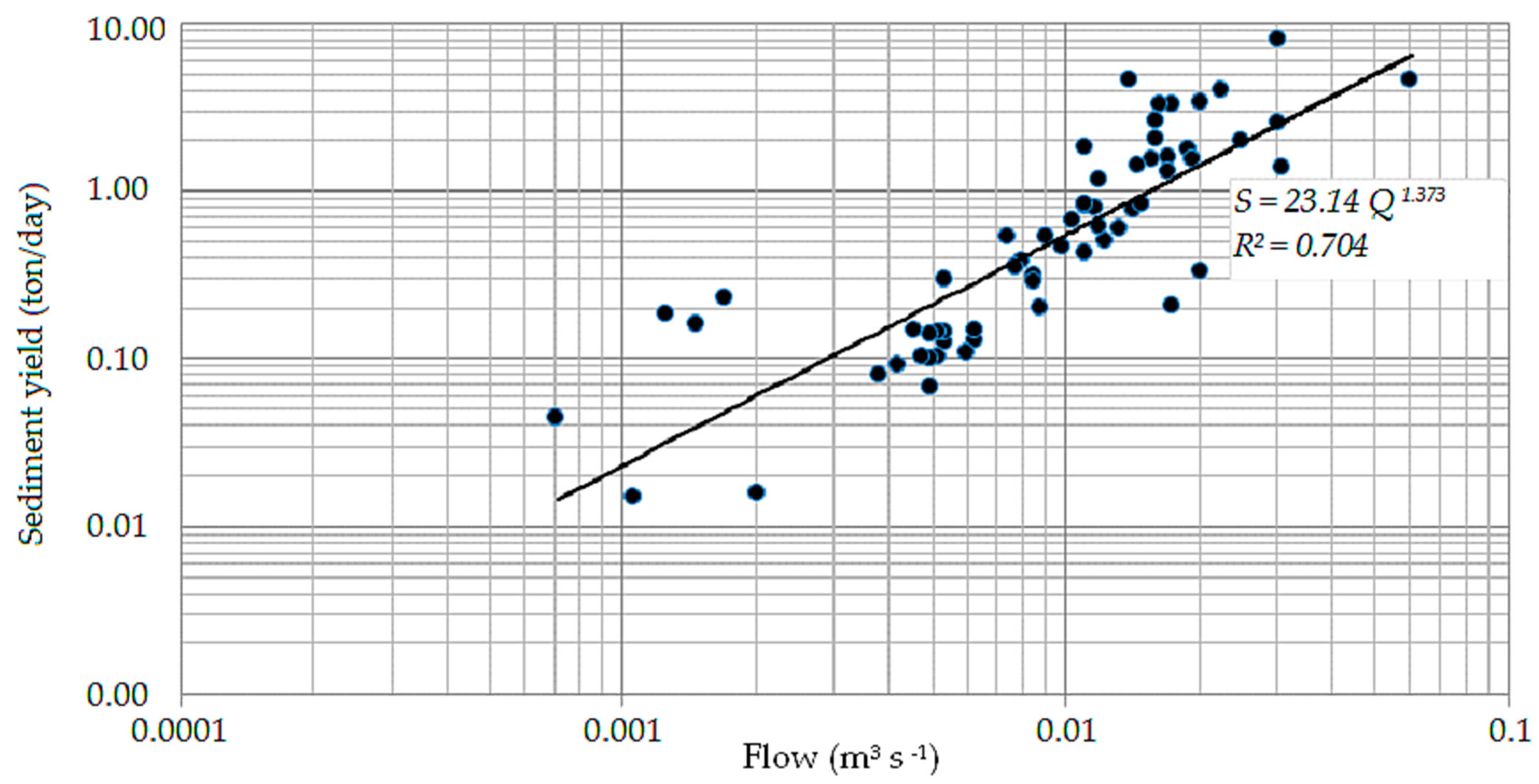
2.6. Sediment Rating Curve

The rating curve was developed to estimate continuous sediment concentration data from limited observations in a time series that assisted in estimating annual average sediment delivery into the reservoir. However, the rating curve only provides lump-sum estimates of sediment on the basin outlet, failing to provide the rate and magnitude of sediment erosion for each sub-catchment. This way, it is challenging to use a rating curve to identify erosion hot spot areas for watershed management and future intervention strategies.
The SWAT model, on the other hand, provides an efficient way to assess the spatial variability of sediment yield across each subbasin and quantify the amount of sediment delivery into the reservoir. In this regard, SWAT provides an implication regarding to what extent management interventions are required to meet sediment reduction targets, providing an improved understanding of catchment processes and responses to anthropogenic and natural stressors in mixed land use catchments subjected to upstream land disturbances.
A continuous time step sediment load data was generated at the Koga-Merawi gauge station from measured streamflow and a sediment rating curve (Figure 2). The sediment-rating curve is related to the river discharge and sediment concentration or load [56]. The sediment rating curve is plotted to show the average sediment concentration or load as a discharge function averaged daily, monthly, or other periods. The general relationship used to transform the records of discharges into sediment concentration or load using rating curve is:
S = a Q b
S is sediment load in ton/day, Q is the discharge in m3 s −1 and, a and b are regression constants. The measured sediment concentration data collected from the ministry of water and energy (MoWE) hydrology and water quality directorate is converted into sediment load by the formula:
S = 0.0864 ∗ QC
where S is sediment load in ton/day, Q is flow of the stream (m3 s−1), C is sediment concentration (mg L−l) and 0.0864 is a dimensionless coefficient for unit conversion. Following the sediment load computation, a relationship between the continuous (daily time step) measured flow in m3 s−1 and the measured sediment load (ton/day) with 0.704 R2 value.

2.7. Estimation of Sediment Load to the Reservoir

Using empirical trap efficiency techniques, the predicate volume of sediment for the Koga reservoir was estimated. These techniques are based on practical field surveys that determine sediment accumulation rates in reservoirs for many years.
The full supply level reservoir storage was used for this purpose. Since the reservoir capacity changes with time, the trap efficiency was calculated for the beginning and end of the reservoir’s design life with negligible difference in Koga Reservoir. Prediction of the unit weight of the Koga reservoir deposits was estimated by the empirical equation of Lane and Koelzer [57], which estimates sediment density based on age and grain-size distribution of the sediment as:
W t = W 1 + K   l o g ( T )
where Wt is the dry density of deposits after T years of compaction, W1 = unit weight at the end of the first year, lb/ft3 or kg/m3, K = consolidation coefficient of the material (related to particle size and the exposure environment of deposits), and T = age of the deposit.
A sand deposit’s unit weight was considered constant with time. However, clay and silt deposits consolidate by over 200 percent. Based on the characteristics of the sediment (i.e., percent of each material type), the composite unit weight (Wave) of sediment T years after deposition was calculated by:
W a v e = p s W t s + p m W t m + p m c W t c
Ps = percentages of clay, silt, and sand, respectively, of the incoming sediment, subscript s, m, and c stand for sand, silt, and clay. The British Standard grain size classification scale was used for the Koga reservoir. The laboratory analysis results for the grain size distribution of sediments from the watershed is shown in Figure 3. The average sediment composition for clay, silt, and sand is 52.2, 40.9, and 6.9 percent, respectively.
Apart from model watershed prioritization, primary sediment samples were collected from three different locations of the reservoir. The aggregates’ size distribution was analyzed at the river entrance (A); middle of the impounded area (B); and near the dam axis (C). The sediment constituents at each sample location of the reservoir were classified (British Standard) into three groups, with an average particle size diameter of D ≤ 0.002 mm, 0.002 ≤ D ≤ 0.06 mm, and 0.06 < D ≤ 2.00 mm for clay, silt, and sand, respectively (Figure 3). The deposited sediment’s mean particle size consisted of 52.2% clay, 40.9% silt, and 6.9% sand.
The median grain size (D50) is the particle diameter’s value at 50% finer in the cumulative distribution. The grain diameter for which half the sample (by weight) is smaller was found to be 0.0021 mm (A), 0.00042 mm (B), and 0.0018 mm (C). A four-step procedure was followed to determine the sediment distribution as an estimation of the amount of sediment to be distributed, determination of the sediment distribution design curves, computation of the dimensionless function from elevation area and capacity curves at several different pool elevations in the deeper part of the reservoir, and distribution of the specified volume of trapped sediment with the selected curve type (Figure 4).

3. Results and Discussion

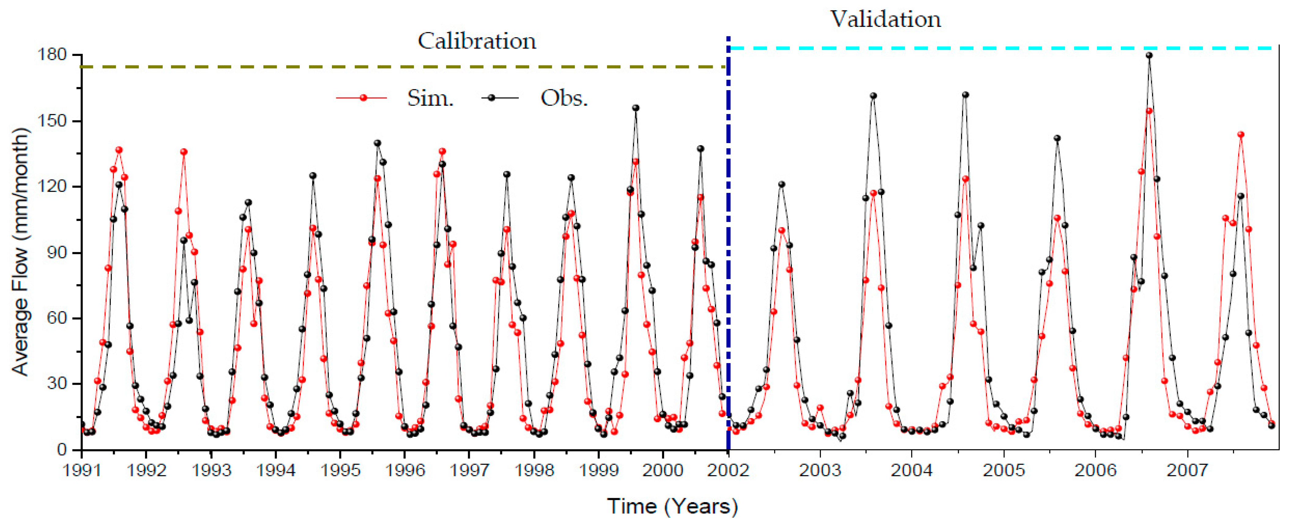
3.1. SWAT Flow Simulation

SWAT model sensitivity analysis (Table 3) was carried out using the SWAT-CUP package to identify the most sensitive flow parameter for ten calibration years (1991 to 2000). This iteration identified ten sensitive parameters, and values were varied iteratively within the allowable ranges until a satisfactory agreement between measured and simulated streamflow was obtained.
The model performance criteria showed good agreement between measured and simulated monthly flows (Table 4) during calibration results with a value of 0.78, 0.82, and 8.45% for Nash-Sutcliffe Efficiency (NSE), correlation coefficient (R2), and percent bias (PBIAS), respectively. Similarly, validation objective functions were in the acceptance range with NSE, R2, and PBIAS values of 0.75, 0.78, and 11.83, respectively (Table 4).
The model slightly over/underestimates some of the peak flows (Figure 5). This may have resulted from input data uncertainty and the weather or flow data quality used to input the model. Some stations have missing weather data, which were left to be estimated and filled by the weather generator.

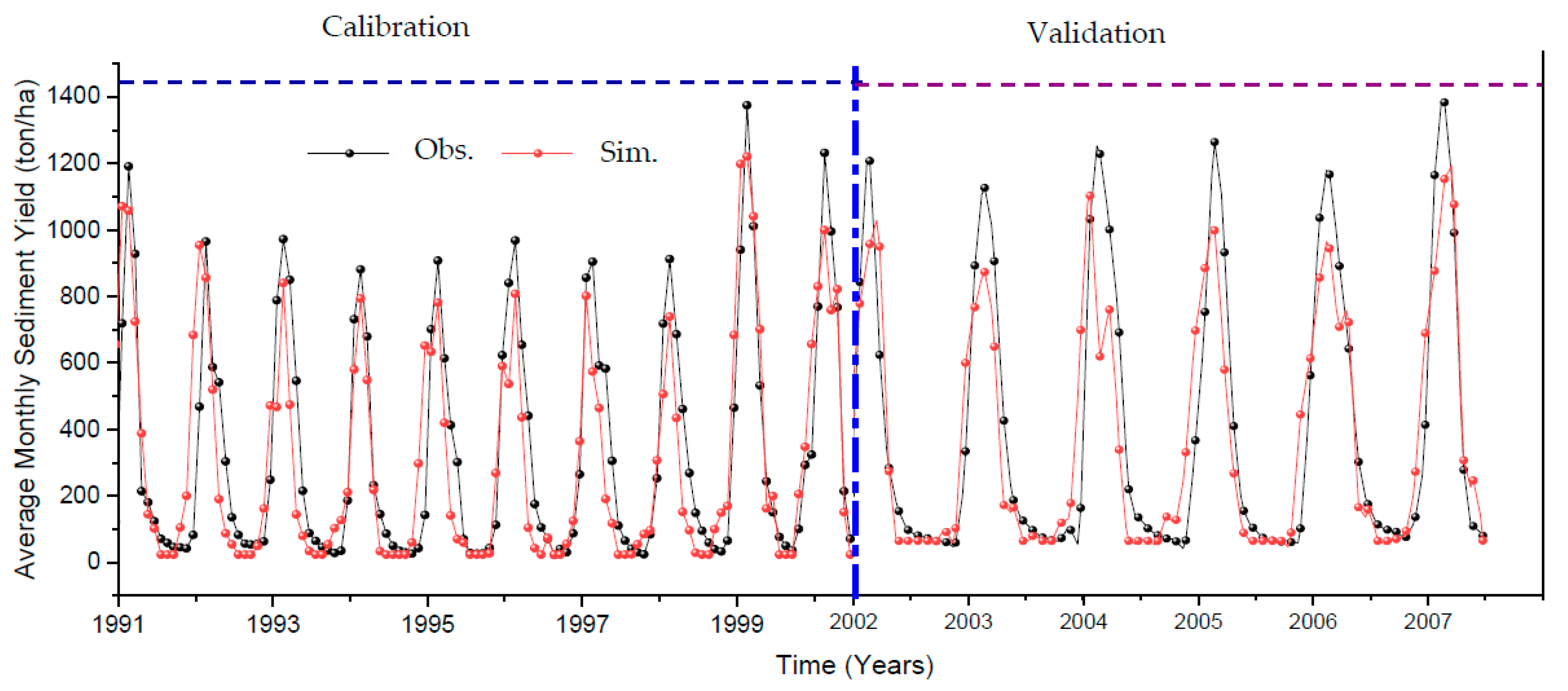
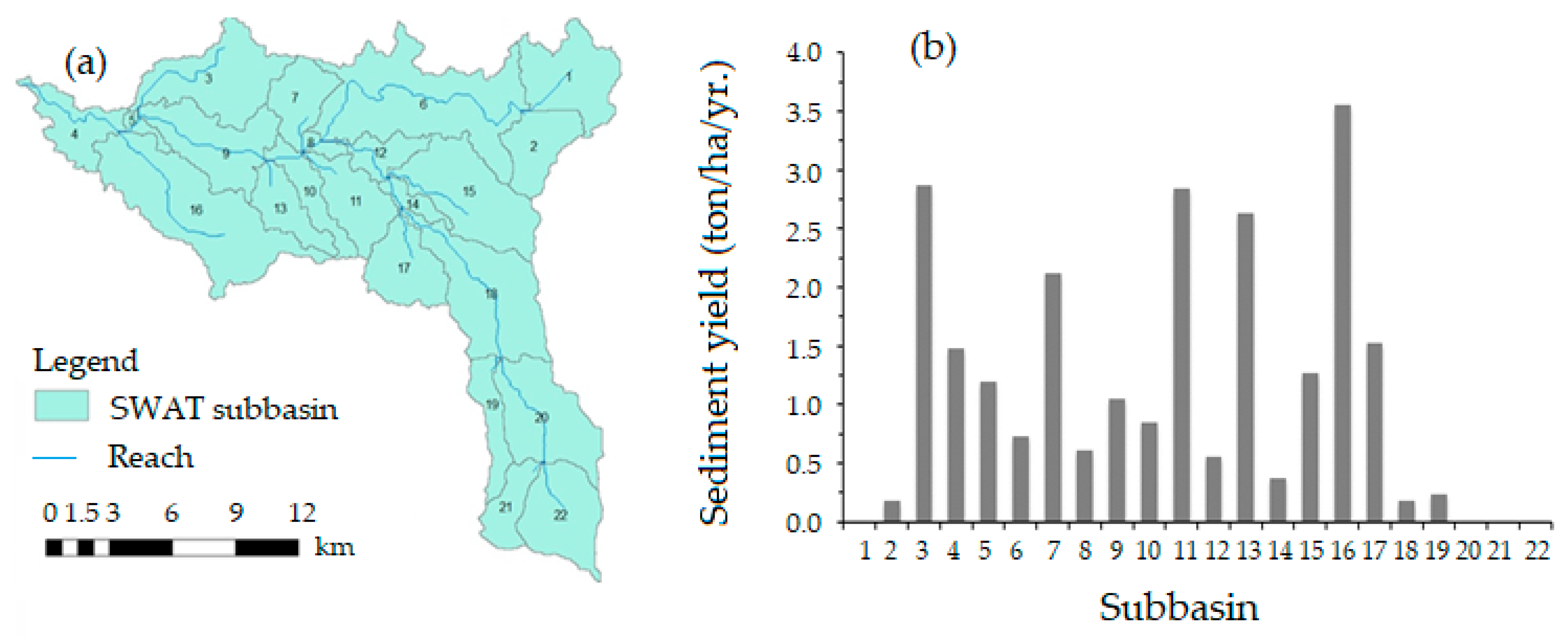
3.2. SWAT Sediment Yield Simulation

The six parameters identified as the most sensitive to affect sediment yields were the USLE support practice factor (USLE P), linear factor for channel sediment routing (SPCON), exponential factor for channel sediment routing (SPEXP), channel erodibility factor (CH EROD), channel cover factor (CH CO), and USLE cover or management factor (USLE C). The USLE support practice factor (USLE P) has been changed to 0.65, the soil loss ratio with a given support practice to the equivalent loss with up and downslope culture. Based on the channel parameters, the linear parameter for determining the maximum quantity of sediment that may be re-entrained during channel sediment routing (SPCON) was set to 0.0015. The exponent value for sediment re-entrained in channel sediment routing (SPEXP) was adjusted to 0.1.
After adjustment of all the above parameters, the monthly simulations for calibration resulted in a coefficient of determination (R2), Nash-Sutcliffe Coefficients (ENS), and percent bias (PBIAS) of 0.72, 0.74, and 10.34%, respectively (Table 5). The observed and simulated sediment load monthly for the calibration period show a slight model overestimate for April 1991, July 1992, and October 2000 (Figure 6). Validation of sediment yield was carried out from 1 January 2001 to 31 December 2007 with one-year initialization.
The statistical values for the monthly sediment yield estimation in the validation period result in R2, ENS, and PBIAS values of 0.69, 0.72, and 6.91%, respectively (Table 5). The observed and simulated sediment yield in the validation period shows slight model underestimation for the high flow periods. The model simulation and the observed sediment yield have established a good fit in low and medium flow periods. They have shown a good fit, under, and overestimation in some months (Figure 6).
The analysis was made to identify the erosion hotspot area and the primary source of sediment yield among the 22 contributing sub-watersheds for a period of nineteen years (1991–2007). The nineteen-year annual average measured suspended sediment generated from the sediment-rating curve was 62,600 tons/yr. The simulated annual average suspended sediment yield by the SWAT model was 58,010 tons/yr. The distribution of sediment yield for the Koga watershed as simulated by the model is presented in Figure 7. This Figure allows us to identify the sub-watersheds which are producing high sediment yields. It is shown that 17 SWAT sub-watersheds produce average annual sediment yields ranging from 0–2.0 ton/ha/yr in low land, and 2–4 ton/ha/yr in high land areas.
Soil formation rates are critical for determining the rate of soil loss, the maximum amount of soil loss that may be tolerated, and the possibility for soil regeneration once soil erosion has been controlled [58]. A similar study on soil formation rates in Ethiopia’s different agro-ecological zones indicates that the range of tolerable soil loss levels for Ethiopia’s agro-ecological zones was 2 to 18 t/ha/yr [58]. Our study result supported previous sediment yield values obtained from other studies [32]. SWAT model results showed a variation in sediment yield from HRU to HRU as a result of spatial variation of main landscape datasets, soil, and land use in each HRU. Sub-watersheds 3, 7, 11, 13, and 16 produced the highest sediment yield, with values ranging from 2.2–3.55 ton ha−1 yr−1 showing more exposure to erosion. The remaining sub-watersheds showed moderate sediment yields, which may be an indication of good management practices.
To manage soil erosion, assessing the state of the watershed and adopting watershed interventions is a key first step [58]. In the Koga watershed, farmers’ purposeful actions, poor working conditions, rodent infestations, land occupancy by physical measures, waterlogging issues, plowing inconveniently, and free grazing were cited as the major causes of destruction of constructed/established physical soil and water conservation measures. As a result, the Bureau of Rural Development has implemented and erected terraces, cut-off drains, canals, and check dams as part of assessing the state of physical soil and water conservation measures (Figure 8).

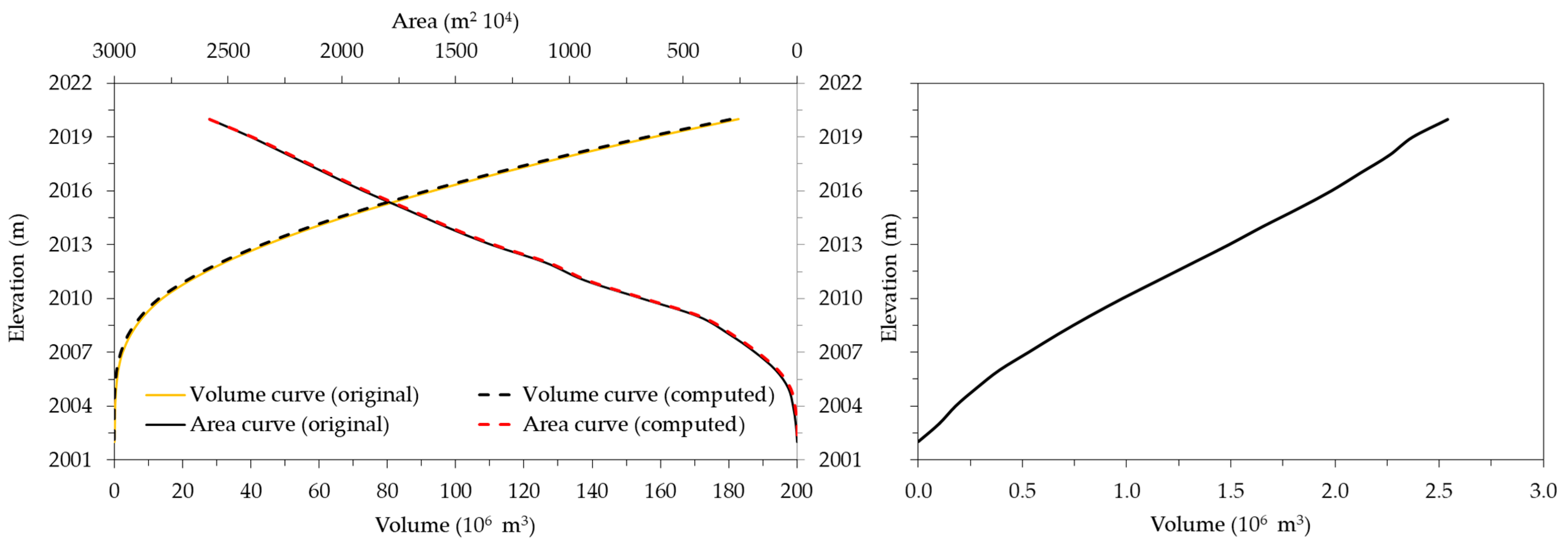
3.3. Empirical Reservoir Sedimentation

For the calculation of sediment accumulation into the reservoir, and sediment inflow into the reservoir was generated using the sediment rating curve equation, which resulted in an average annual sediment load of 62,610.08 tons/yr at the dam site. The annual average sediment load estimated from the rating curve equation was relatively higher than the result from the design report; a value of 57,665 tons/yr [59]. Daily discharge may compute the sediment load when using the power function, sensitive to slight variations. Before estimating reservoir sedimentation amounts using the empirical area reduction method and computation of sediment distribution (Table 6), the trap efficiency (η), grain size, unit weight, and sediment distribution were analyzed. The long-term trap efficiency (η) in impounded reservoirs is based on the correlation between capacity and inflow ratios (C : I). The Koga reservoir’s total capacity is 83.1 Mm3. The capacity-inflow ratio is 0.480, and the trap efficiency of the reservoir from the Brune curve is read as 96%. From the laboratory analysis, the percent composition of sediment (grain Size) around the Koga watershed is a mixture of clay (52.23), silt (40.86), and sand (9.60). The unit dry weight of Koga reservoir sediment deposition at the end of the reservoir’s design life based on age and grain size distribution of the sediment from the empirical equation of Lane and Koelzer [57] was found to be 1.16 ton/m3.
The distribution of sediment at Koga reservoir has a moderate drawdown operation manner with a flood plain foothill shape. The specified volume of trapped sediment was distributed within the reservoir for the selected type ll curve. The values for relative sediment area (an of 0.468) (Column 6) at each relative depth (p of 0.056) were determined to compute a reduction factor (Ao/a) value of 13.25 ha estimated by dividing 6.2 to 0.468.
The area adjustment factor was multiplied by the relative sediment area (column 6) at each level above the revised zero-capacity elevation to obtain the area occupied by sediment at each pool height (column 7) (Table 6). The sediment pool area matches the original pool area in the whole sediment section of the reservoir, which extends from the new zero-capacity elevation to the original bottom. To calculate the sediment volume for each step, the end area technique was used to increase above the new zero-capacity elevation (column 8). By subtracting the sediment area (column 7) and cumulative sediment volume (column 9) from the original area and capacity values, the revised area and capacity curves (columns 10 and 11) were generated (columns 2 and 3).
In 50 years of the reservoir’s design life, the accumulation and distribution of sediment in the Koga reservoir in different elevations and corresponding value are shown in Table 6, column (1) and column (9), respectively. The cumulative volume of sediment in the reservoir at the elevation of 2020 will be 2.54 Mm3. The original survey of Koga reservoir stage-capacity and stage-area relationship curves (Figure 9, left) were revised after 50 years of the design life of the reservoir, due to changes in the accumulation and distribution of sediment Table 6, columns (1), (10) and (11). Reservoir sediment distribution and accumulation after 50 years of design life is also presented (Figure 9, right; Table 6 column (1) and column (9)).
There is only a slight shift between the curves. However, the projected change in the reservoir capacity and water surface area due to sediment deposition during the dam’s operational period is not considered significant while employing the Area Reduction Method (ARM). This could be true if land management practices are factored in. When appropriate and timely watershed management strategies were applied to selected sediment erosion-prone areas (erosion hotspot areas), reservoir sedimentation did not show a substantial change. However, this condition was strictly hinged on timely application and extent of land use management and interventions to offset reservoir sedimentation.

4. Conclusions

Anthropogenic activity and resulting landscape disturbance have significantly enhanced soil erosion rates in Ethiopia. The study was conducted in a catchment characterized by spatiotemporal variability in land use that affects the hydrological function of river systems, mainly shifting the generation and transport of streamflow and sediment loads. Besides SWAT model-based sediment yield predictions, we used a rating curve technique to predict suspended sediment load. Even though gross erosion estimations and field observations can detect soil erosion and sedimentation, quantifiable data and information are needed to build alternative watershed management plans at the sub-watershed level. The goal of this study was to characterize the Koga watershed, identify the factors causing soil erosion and reservoir storage capacity loss, identify potential sediment source areas, provide measurable data on sediment yield and reservoir sedimentation, and recommend possible remedial measures to prevent soil erosion in the Koga Watershed.
We utilized the SWAT model to analyze the spatial variability of sediment output and identify erosion hotspot regions for future watershed management. Standard calibration and validation statistics were used to assess the model’s performance. Comparison of modeled and observed monthly streamflow datasets resulted from R2, ENS, and PBIAS values of 0.82, 0.78, and 8.45% for calibration (1992–2000) and 0.78, 0.75, 11.83% for validation periods (2002–2007), respectively. Statistical model evaluation criteria for the monthly sediment yield simulation resulted in an R2, ENS, and PBIAS values of 0.75, 0.73, and 7.8% for calibration and 0.80, 0.79, and 6.4% for validation periods, respectively. For both flow and sediment simulations, model statistical performance evaluation criteria fell within the acceptable limits. There was good agreement between simulated and measured datasets.
In conclusion, the paper assessed changes in the hydrology of a hillslope-dominated catchment over the past decades. It highlighted the importance of soil and water conservation measures to meet sediment load targets. The sediment-rating curve indicated an annual average measured suspended sediment load of 62,610.08 tons, and 58,012.87 tons of mean annual sediment yield prediction was indicated from SWAT model outputs. Findings would benefit policymakers regarding land, water management decisions, and serve as a prototype for other catchments where land-use change may be implemented.

Author Contributions

Credit author statement: Conceptualization, G.T.A.; Methodology, G.T.A., E.Z.T., M.A.J.; Resources, G.T.A.; Supervision, S.S.D., A.M.M.; Writing—original draft, G.T.A.; Writing—review and editing, G.T.A., A.K., M.A.J., S.M.S., A.M.S., E.Z.T., M.H.D., S.A.B., S.S.D., J.J. and A.M.M.; funding acquisition, G.T.A. All authors have read and agreed to the published version of the manuscript.

Funding

The authors disclose receipt of financial support for this article’s research and publication. This research was funded by Bahir Dar University-Blue Nile Water Institute under the project “Remote sensing approaches to access drought severity from multi-temporal GIMMS NDVI, rainfall and PDSI interactions for future drought monitoring (Grant number: 1/26971/1.11.10)”.

Acknowledgments

Gebiaw T. Ayele would like to thank Dagnachew Aklog, Tesfaye Shiferaw, Asegdew Gashaw, Mamaru A. Moges, Seifu A. Tilahun; Goraw Goshu, and Elias Simie of Bahir Dar University–Blue Nile Water Institute. Alban Kuriqi acknowledges the support of the Portuguese Foundation for Science and Technology (FCT) through the project PTDC/CTA-OHR/30561/2017 (WinTherface).

Conflicts of Interest

The authors declare no conflict of interest.

References

  1. Jaiyeola, A.T.; Bwapwa, J.K. Dynamics of sedimentation and use of genetic algorithms for estimating sediment yields in a river: A critical review. Nat. Resour. Model. 2015, 28, 207–218. [Google Scholar] [CrossRef]
  2. Pavanelli, D.; Pagliarani, A. SW—Soil and Water: Monitoring water flow, turbidity and suspended sediment load, from an Apennine Catchment Basin, Italy. Biosyst. Eng. 2002, 83, 463–468. [Google Scholar] [CrossRef]
  3. Russell, M.; Walling, D.; Hodgkinson, R. Suspended sediment sources in two small lowland agricultural catchments in the UK. J. Hydrol. 2001, 252, 1–24. [Google Scholar] [CrossRef]
  4. Gao, P.; Pasternack, G. Dynamics of suspended sediment transport at field-scale drain channels of irrigation-dominated watersheds in the Sonoran Desert, southeastern California. Hydrol. Process. Int. J. 2007, 21, 2081–2092. [Google Scholar] [CrossRef]
  5. Gao, P.; Puckett, J. A new approach for linking event-based upland sediment sources to downstream suspended sediment transport. Earth Surf. Process. Landf. 2012, 37, 169–179. [Google Scholar] [CrossRef]
  6. Sadeghi, S.; Mizuyama, T.; Miyata, S.; Gomi, T.; Kosugi, K.; Fukushima, T.; Mizugaki, S.; Onda, Y. Determinant factors of sediment graphs and rating loops in a reforested watershed. J. Hydrol. 2008, 356, 271–282. [Google Scholar] [CrossRef]
  7. Elosegi, A.; Díez, J.R.; Flores, L.; Molinero, J. Pools, channel form, and sediment storage in wood-restored streams: Potential effects on downstream reservoirs. Geomorphology 2017, 279, 165–175. [Google Scholar] [CrossRef]
  8. Hamed, Y.; Albergel, J.; Pépin, Y.; Asseline, J.; Nasri, S.; Zante, P.; Berndtsson, R.; El-Niazy, M.; Balah, M. Comparison between rainfall simulator erosion and observed reservoir sedimentation in an erosion-sensitive semiarid catchment. CATENA 2002, 50, 1–16. [Google Scholar] [CrossRef]
  9. Nyssen, J.; Poesen, J.; Moeyersons, J.; Haile, M.; Deckers, J. Dynamics of soil erosion rates and controlling factors in the Northern Ethiopian Highlands–towards a sediment budget. Earth Surf. Process. Landf. 2008, 33, 695–711. [Google Scholar] [CrossRef] [Green Version]
  10. López-Tarazón, J.A.; Batalla, R.J.; Vericat, D.; Francke, T. Suspended sediment transport in a highly erodible catchment: The River Isábena (Southern Pyrenees). Geomorphology 2009, 109, 210–221. [Google Scholar] [CrossRef]
  11. Da Silva, R.M.; Santos, C.A.; e Silva, L.P.; da Costa Silva, J.F.C. Evaluation of soil loss in Guaraíra basin by GIS and remote sensing based model. J. Urban Environ. Eng. 2007, 1, 44–52. [Google Scholar] [CrossRef]
  12. Turner, B. The Earth as Transformed by Human Action; Cambridge University Press: Cambridge, UK, 1990. [Google Scholar]
  13. Eswaran, H.; Lal, R.; Reich, P. Land degradation: An overview. In Responses to Land Degradation; Bridges, E.M., Hannam, I.D., Oldeman, L.R., Pening de Vries, F.W.T., Scherr, S.J., Sompatpanit, S., Eds.; Oxford Press: New Delhi, India, 2001; pp. 20–35. [Google Scholar]
  14. Shiferaw, B.; Holden, S. Soil erosion and smallholders’ conservation decisions in the highlands of Ethiopia. World Dev. 1999, 27, 739–752. [Google Scholar] [CrossRef]
  15. BCEOM, F.E. Abbay River Basin Integrated Development Master Plan. Project, Volume Xiii—Environment; Ministry of Water Resource: Addis Ababa, Ethiopia, 1998.
  16. Schleiss, A.J.; Franca, M.J.; Juez, C.; De Cesare, G. Reservoir sedimentation. J. Hydraul. Res. 2016, 54, 595–614. [Google Scholar] [CrossRef]
  17. Marttila, H.; Kløve, B. Dynamics of erosion and suspended sediment transport from drained peatland forestry. J. Hydrol. 2010, 388, 414–425. [Google Scholar] [CrossRef]
  18. Devlin, D.; Dhuyvetter, K.; McVay, K.; Kastens, T.; Rice, C.; Janssen, K.; Pierzynski, G. Water Quality Best Management Practices, Effectiveness, and Cost for Reducing Contaminant Losses from Cropland; Publication MF-2572, Kansas State University: Manhattan, KS, USA, 2003. [Google Scholar]
  19. Oehy, C.D.; Schleiss, A.J. Control. of turbidity currents in reservoirs by solid and permeable obstacles. J. Hydraul. Eng. 2007, 133, 637–648. [Google Scholar] [CrossRef]
  20. Awulachew, S.B.; Erkossa, T.; Smakhtin, V.; Fernando, A. Improved Water and Land Management in the Ethiopian highlands: Its impact on downstream stakeholders dependent on the Blue Nile. In Proceedings of the Intermediate Results Dissemination Workshop, the International Livestock Research Institute (ILRI), Addis Ababa, Ethiopia, 5–6 February 2009. Summary report, abstracts of papers with proceedings on CD-ROM. 2009: IWMI. [Google Scholar]
  21. Gao, P.; Josefson, M. Event-based suspended sediment dynamics in a central New York watershed. Geomorphology 2012, 139, 425–437. [Google Scholar] [CrossRef]
  22. Assfaw, A.T. Modeling Impact of Land Use Dynamics on Hydrology and Sedimentation of Megech Dam Watershed, Ethiopia. Sci. World J. 2020. [Google Scholar] [CrossRef]
  23. Leibowitz, S.G.; Wigington, P.J., Jr.; Schofield, K.A.; Alexander, L.C.; Vanderhoof, M.K.; Golden, H.E. Connectivity of streams and wetlands to downstream waters: An integrated systems framework. JAWRA J. Am. Water Resour. Assoc. 2018, 54, 298–322. [Google Scholar] [CrossRef]
  24. Fritz, K.M.; Schofield, K.A.; Alexander, L.C.; McManus, M.C.; Golden, H.E.; Lane, C.R.; Kepner, W.G.; LeDuc, S.D.; DeMeester, J.E.; Pollard, A.I. Physical and chemical connectivity of streams and riparian wetlands to downstream waters: A synthesis. JAWRA J. Am. Water Resour. Assoc. 2018, 54, 323–345. [Google Scholar] [CrossRef]
  25. El-Khoury, A.; Seidou, O.; Lapen, D.R.; Que, Z.; Mohammadian, M.; Sunohara, M.; Bahram, D. Combined impacts of future climate and land use changes on discharge, nitrogen and phosphorus loads for a Canadian river basin. J. Environ. Manag. 2015, 151, 76–86. [Google Scholar] [CrossRef] [Green Version]
  26. Harms, T.K.; Grimm, N.B. Hot spots and hot moments of carbon and nitrogen dynamics in a semiarid riparian zone. J. Geophys. Res. Biogeosci. 2008, 113. [Google Scholar] [CrossRef] [Green Version]
  27. Arnold, J.G.; Allen, P. Estimating hydrologic budgets for three Illinois watersheds. J. Hydrol. 1996, 176, 57–77. [Google Scholar] [CrossRef]
  28. Bisantino, T.; Bingner, R.; Chouaib, W.; Gentile, F.; Trisorio Liuzzi, G. Estimation of runoff, peak discharge and sediment load at the event scale in a medium-size Mediterranean watershed using the AnnAGNPS model. Land Degrad. Dev. 2015, 26, 340–355. [Google Scholar] [CrossRef]
  29. Jeong, J.; Kannan, N.; Arnold, J.; Glick, R.; Gosselink, L.; Srinivasan, R. Development and integration of sub-hourly rainfall–runoff modeling capability within a watershed model. Water Resour. Manag. 2010, 24, 4505–4527. [Google Scholar] [CrossRef]
  30. Assefa, T.T.; Jha, M.K.; Tilahun, S.A.; Yetbarek, E.; Adem, A.A.; Wale, A. Identification of erosion hotspot area using GIS and MCE technique for koga watershed in the upper blue Nile Basin, Ethiopia. Am. J. Environ. Sci. 2015, 11, 245. [Google Scholar] [CrossRef] [Green Version]
  31. Reynolds, B. Variability and change in Koga reservoir volume, Blue Nile, Ethiopia: Variabilitet och förändring i Kogadammens vattenvolym, Blå Nilen, Etiopien. Digitala Vetenskapliga Arkivet 2012. [Google Scholar]
  32. Ayele, G.T.; Teshale, E.Z.; Yu, B.; Rutherfurd, I.D.; Jeong, J. Streamflow and sediment yield prediction for watershed prioritization in the Upper Blue Nile River Basin, Ethiopia. Water 2017, 9, 782. [Google Scholar] [CrossRef] [Green Version]
  33. MoWR. Spatial and Hydrological Data; Ministry of Water Resources, The Federal Democratic Republic of Ethiopia: Addis Abeba, Ethiopia, 2009.
  34. Gassman, P.W.; Reyes, M.R.; Green, C.H.; Arnold, J.G. The soil and water assessment tool: Historical development, applications, and future research directions. Trans. ASABE 2007, 50, 1211–1250. [Google Scholar] [CrossRef] [Green Version]
  35. Arnold, J.G.; Srinivasan, R.; Muttiah, R.S.; Williams, J.R. Large area hydrologic modeling and assessment part I: Model development 1. JAWRA J. Am. Water Resour. Assoc. 1998, 34, 73–89. [Google Scholar] [CrossRef]
  36. Chanasyk, D.; Mapfumo, E.; Willms, W. Quantification and simulation of surface runoff from fescue grassland watersheds. Agric. Water Manag. 2003, 59, 137–153. [Google Scholar] [CrossRef]
  37. Arnold, J.G.; Muttiah, R.S.; Srinivasan, R.; Allen, P.M. Regional estimation of base flow and groundwater recharge in the Upper Mississippi river basin. J. Hydrol. 2000, 227, 21–40. [Google Scholar] [CrossRef]
  38. Me, W.; Abell, J.M.; Hamilton, D.P. Modelling Water, sediment and Nutrient Fluxes from a Mixed Land-Use Catchment in New Zealand: Effects of Hydrologic Conditions on SWAT Model Performance; European Geosciences Union: Munich, Germany, 2015. [Google Scholar]
  39. Neitsch, S.; Arnold, J.G.; Kiniry, J.R.; Srinivasan, R.; Williams, J.R. Soil and Water Assessment Tool User’s Manual; Blackland Research Center: Temple, TX, USA, 2000. [Google Scholar]
  40. NMSA. World Weather Information Service; NMSA: Addis Abeba, Ethiopia, 2009. [Google Scholar]
  41. Neitsch, S.L.; Arnold, J.G.; Kiniry, J.R.; Williams, J.R. Soil and Water Assessment Tool Theoretical Documentation Version 2009; Texas Water Resources Institute: Austin, TX, USA, 2011. [Google Scholar]
  42. Morris, G.L.; Fan, J. Reservoir Sedimentation Handbook: Design and Management of Dams, Reservoirs, and Watersheds for Sustainable Use; McGraw Hill Professional: New York, NY, USA, 1998. [Google Scholar]
  43. Summer, W.; Klaghofer, E.; Abi-Zeid, I.; Villeneuve, J.P. Critical reflections on long term sediment monitoring programmes demonstrated on the Austrian Danube. Eros. Sediment Trans. Monit. Prog. River Basins 1992, 255–262. [Google Scholar]
  44. Ndomba, P.M.; Mtalo, F.W.; Killingtveit, Å. A guided SWAT model application on sediment yield modeling in Pangani river basin: Lessons learnt. J. Urban Environ. Eng. 2008, 2, 53–62. [Google Scholar] [CrossRef]
  45. Yesuf, H.M.; Assen, M.; Alamirew, T.; Melesse, A.M. Modeling of sediment yield in Maybar gauged watershed using SWAT, northeast Ethiopia. Catena 2015, 127, 191–205. [Google Scholar] [CrossRef]
  46. Pourghasemi, H.R.; Sadhasivam, N.; Kariminejad, N.; Collins, A.L. Gully erosion spatial modelling: Role of machine learning algorithms in selection of the best controlling factors and modelling process. Geosci. Front. 2020, 11, 2207–2219. [Google Scholar] [CrossRef]
  47. Williams, J.R. The EPIC Model. Computer Models of Watershed Hydrology; Water Resources Publications: Highlands Ranch, CO, USA, 1995; pp. 909–1000. [Google Scholar]
  48. Wischmeier, W.H.; Smith, D.D. Predicting Rainfall Erosion Losses: A Guide to Conservation Planning; Department of Agriculture, Science and Education Administration: Seattle, WA, USA, 1978.
  49. Abbaspour, K.C.; Rouholahnejad, E.; Vaghefi, S.; Srinivasan, R.; Yanga, H.; Kløve, B. A continental-scale hydrology and water quality model for Europe: Calibration and uncertainty of a high-resolution large-scale SWAT model. J. Hydrol. 2015, 524, 733–752. [Google Scholar] [CrossRef] [Green Version]
  50. Moriasi, D.N.; Arnold, J.G.; Van Liew, M.W.; Bingner, R.L.; Harmel, R.D.; Veith, T.L. Model evaluation guidelines for systematic quantification of accuracy in watershed simulations. Trans. ASABE 2007, 50, 885–900. [Google Scholar] [CrossRef]
  51. Krause, P.; Boyle, D.; Bäse, F. Comparison of different efficiency criteria for hydrological model assessment. Adv. Geosci. 2005, 5, 89–97. [Google Scholar] [CrossRef] [Green Version]
  52. McCuen, R.H.; Knight, Z.; Cutter, A.G. Evaluation of the Nash–Sutcliffe efficiency index. J. Hydrol. Eng. 2006, 11, 597–602. [Google Scholar] [CrossRef]
  53. Boskidis, I.; Gikas, G.D.; Sylaios, G.K.; Tsihrintzis, V.A. Hydrologic and water quality modeling of lower Nestos river basin. Water Resour. Manag. 2012, 26, 3023–3051. [Google Scholar] [CrossRef]
  54. Legates, D.R.; McCabe, G.J., Jr. Evaluating the use of “goodness-of-fit” measures in hydrologic and hydroclimatic model validation. Water Resour. Res. 1999, 35, 233–241. [Google Scholar] [CrossRef]
  55. Guinot, V.; Cappelaere, B.; Delenne, C.; Ruellandet, D. Towards improved criteria for hydrological model calibration: Theoretical analysis of distance-and weak form-based functions. J. Hydrol. 2011, 401, 1–13. [Google Scholar] [CrossRef]
  56. Clarke, R.T. Statistical Modelling in Hydrology; John Wiley & Sons: Hoboken, NJ, USA, 1994. [Google Scholar]
  57. Lane, E.; Koelzer, V.A. Density of Sediments Deposited in Reservoirs, a Case Study of Methods Used in Measurement and Analysis of Sediment Loads in Streams, Report No. 9, Interagency Committee on Water Resources; University of Iowa: Iowa City, IA, USA, 1943. [Google Scholar]
  58. Hurni, H. Soil Conservation Manual for Ethiopia: Field Guide for Conservation Implementation; Ministry of Agriculture: Addis Abeba, Ethiopia, 1985.
  59. MacDonald, M.; WWDSE. Koga Irrigation Project, Irrigation and Drainage Design Report; WWDSE: Addis Ababa, Ethiopia, 2005. [Google Scholar]
Figure 1. Location map of the study area: the geographical setting of the Koga watershed (a) and location of the study area in the Abbay basin with a network of rivers and streams (b); and country map of Africa (c).
Water 13 03374 g001
Figure 2. Sediment rating curve of Koga River at Koga-Merawi gauge station.
Water 13 03374 g002
Figure 3. Grain size distribution curve at Koga River inlet into the reservoir (A), at the saddle dam near the middle of the reservoir (B), and near the central dam axis (C).
Water 13 03374 g003
Figure 4. Koga reservoir characteristics (stage-capacity and stage-area relationship).
Water 13 03374 g004
Figure 5. Observed and simulated monthly flow hydrograph for calibration (1991–2000) and validation periods (2002–2007).
Water 13 03374 g005
Figure 6. Monthly calibration (1991–2000) and validation (2002–2007) results of measured and simulated sediment yield.
Water 13 03374 g006
Figure 7. SWAT classified subbasins for prioritization (a) and SWAT simulated annual sediment yield in Koga subbasins (b).
Water 13 03374 g007
Figure 8. Existing structural soil and water conservation measures in the watershed (photo by Engidasew Z. Teshale, 2012).
Water 13 03374 g008
Figure 9. The original and adjusted stage-capacity and stag-earea curves for Koga reservoir (left) and reservoir sediment accumulation within fifty years design period of the dam (right).
Water 13 03374 g009
Table 1. Data source and description of data used to configure SWAT model.
DataApplicationData Use and DescriptionSource
3 stations
meteorological data
Meteorological forcingDaily max., and min., temperature, humidity, radiation, wind speed, and precipitation.NMSA
DEM and digitized stream networkWatershed delineation30 m resolution to define slope classes.MoWR
Land useDefining HRUs30 m resolution, six basic land-cover classes.MoWR
Soil characteristicsDefining HRUs30 m resolution, nine soil types.MoWR
Table 2. Classical objective functions, characteristics, function category, equatio n, and performance classification ratings.
Statistical Efficiency CriterionModel Performance Ratings
Objective FunctionCharacteristicsFunction CategoryStatistic EquationReferenceValue RangePerformance ClassificationReferences
ENSMost common; emphasize on high flows; neglect the low flowsDistance-based
N S E = 1 [ i = 1 n ( Q m Q s ) 2 i = 1 n ( Q m Q ¯ m ) 2 ]
[51,52]0.75 < ENS ≤ 1Very good[50,53]
0.65 < ENS ≤ 0.75Good
0.5 < ENS ≤ 0.65Satisfactory
0.4 < ENS ≤ 0.5Acceptable
ENS ≤ 0.4Unsatisfactory
R2Emphasize on high flowsWeak form-based
R 2 = [ i = 1 n [ ( Q m ,   i Q ¯ m ) ( Q s ,   i Q ¯ s ) ] i = 1 n ( Q m ,   i Q ¯ m ) 2 i = 1 n ( Q s ,   i Q ¯ s ) 2 ] 2  
[52,54]0.7 < R2 < 1Very good[50]
0.6 < R2 < 0.7Good
0.5 < R2 < 0.6Satisfactory
R2 < 0.5Unsatisfactory
±PBIASMonotony;
cannot be used alone
Weak form-based
PBIAS = [ i = 1 n ( Y o b s Y s i m ) i = 1 n ( Y o b s ) ] 100 %
[55]PBIAS < ±10Very good[54]
±10 ≤ PBIAS < ±15Good
±15 ≤ PBIAS < ±25Satisfactory
PBIAS ≥ ±25Unsatisfactory
Note: in Equations (5)–(7), n is the number of pairs of measured and simulated variables, i is the time series of the measured and simulated pairs; s and m denote simulated and measured datasets, respectively, and the bar stands for average.
Table 3. Initial and final calibrated flow parameter values.
Parameter DescriptionParameter CodeRangeInitial ValueAdjusted Value
Available water capacity (mm water/mm soil)SOL_AWC±25%**12%
Soil Depth (mm)SOL_Z±25%**−10%
Initial SCS CN II valueCN2±25%*14%
Baseflow Alpha factor (days)ALPHA_BF0–10.0480.048
Threshold water depth in shallow
aquifer for flow
GWQMN0–50000.02500
Manning’s N value for the main channelCh_N20–10.0140.014
Effective hydraulic conductivity
in main channel alluvium
Ch_K20–15000
Soil evaporation compensation factorESCO0–10.950.40
Average slope Steepness (m/m)SLOPE±25%**10%
Groundwater percolation delay(day)GW_DELAY±10%*31
* Indicates SWAT default parameter values for each land use and soil type in each sub-basin; ** indicates initial parameter values from field measurements and the literature review.
Table 4. Monthly measured and simulated streamflow calibration–validation statistics.
Monthly SimulationMean Annual Streamflow (m3/s)Model Performance
ObservedSimulatedNSER2PBIAS (%)
Calibration (1991–2000)5.314.860.780.828.45
Validation (2002–2007)4.684.130.750.7811.83
Table 5. Calibration and validation statistics of observed and simulated average sediment load.
Monthly SimulationModel Performance
NSER2PBIAS (%)
Calibration (1991–2000)0.730.757.8
Validation (2002–2007)0.800.796.4
Table 6. Empirical area reduction method; computation of sediment distribution at Koga reservoir.
Elevation (m)OriginalF ValueRelativeComputed Sed. DistributionRevised
Area
(Ha)
Volume
(m3 106)
Depth
(p)
Area
(ha)
Area
(ha)
V. incre.
(106 m3)
C. Vol.
(106 m3)
Area
(ha)
Volume
(106 m3)
(1)(2)(3)(4)(5)(6)(7)(8)(9)(10)(11)
20202582182.9 1.0000.00.00.052.542582.0180.5
20192400158.0 0.9440.7369.80.112.372390.6155.6
20182236134.8 0.8890.94512.50.132.262222.2132.5
20172072113.3 0.8331.07514.20.152.122057.1111.2
2016190693.4 0.7781.16315.40.161.981890.391.4
2015172475.2 0.7221.22216.20.161.821707.973.4
2014154458.9 0.6671.25816.70.171.651527.957.2
2013134544.5 0.6111.27516.90.171.491328.743.0
2012110632.2 0.5561.27616.90.171.321089.630.9
201193222.1 0.5001.26116.70.171.15915.821.0
201068314.0 0.4441.23116.30.160.98667.213.0
20094358.5 0.3891.18615.70.150.82419.87.7
20082984.8 0.3331.12614.90.140.67283.64.1
20071852.40.0000.2781.04913.90.130.53171.61.9
2006941.10.0770.2220.95212.60.120.3981.80.7
2005390.50.2710.1670.83111.00.100.2828.30.2
2004180.20.6790.1110.6779.00.080.189.30.0
20036.20.12.0610.0560.4686.20.100.100.00.0
20020.00.0 0.0000.0000.00.00.00.00.0
Publisher’s Note: MDPI stays neutral with regard to jurisdictional claims in published maps and institutional affiliations.

