A Comparative Study of Water and Bromide Transport in a Bare Loam Soil Using Lysimeters and Field Plots

Abstract

The purpose of this methodological study was to test whether similar soil hydraulic and solute transport properties could be estimated from field plots and lysimeter measurements. The transport of water and bromide (as an inert conservative solute tracer) in three bare field plots and in six bare soil lysimeters were compared. Daily readings of matric head and volumetric water content in the lysimeters showed a profile that was increasingly humid with depth. The hydrodynamic parameters optimized with HYDRUS-1D provided an accurate description of the experimental data for both the field plots and the lysimeters. However, bromide transport in the lysimeters was influenced by preferential transport, which required the use of the mobile/immobile water (MIM) model to suitably describe the experimental data. Water and solute transport observed in the field plots was not accurately described when using parameters optimized with lysimeter data (cross-simulation), and vice versa. The soil’s return to atmospheric pressure at the bottom of the lysimeter and differences in tillage practices between the two set-ups had a strong impact on soil water dynamics. The preferential flow of bromide observed in the lysimeters prevented an accurate simulation of solute transport in field plots using the mean optimized parameters on lysimeters and vice versa.

1. Introduction

For the last few decades, lysimeters have been frequently used to study water dynamics and solute transport in soils [1,2,3]. Lysimeters are large blocks of soil surrounded by walls with their bottom usually exposed to atmospheric pressure. A wide range of methods can be used for their installation [4]. The main differences between lysimeters are usually (i) their size (from less than 1 m³ to 150 m³), (ii) their filling method (reconstituted or undisturbed soil), (iii) their lower limit (atmospheric pressure or controlled matric head), (iv) their instrumentation level, and (v) whether they are weighed or not [5,6,7]. Numerous studies have already been carried out on water content and solute transport with different types of lysimeters [8,9,10,11].

Frequently considered as an intermediate step between laboratory measurements and field observations [12,13], lysimeters are generally exposed to the same climatic conditions as field plots. They are regularly preferred to laboratory soil columns for the determination of soil hydraulic properties [14] and provide a more precise determination of soil hydrodynamic parameters than the inverse modelling method [15,16], which requires exact knowledge of the soil’s boundary conditions [17,18], and is often deemed uncertain when dealing with field plots.

A few authors have already assessed the feasibility of transposing the findings obtained with lysimeters to field soils, either using experiments [19,20] or using simulations [12,21]. Although comparing the different studies is indeed risky because of the disparities observed in the instruments and procedures used, the authors generally call for caution when transposing the results obtained with lysimeters to the field. The main biases are associated with the impact of the conditions at the lower soil boundary, the soil reconstitution during the installation of the lysimeters, as well as the differences in weather conditions or evapotranspiration between the two systems. However, the possibility of transposing results from lysimeters to field soil is still insufficiently studied, with few tangible experimental and numerical results on the differences between the two systems.

To the knowledge of the authors, none of the studies used water dynamics monitoring instruments in both field plots and lysimeters, and examined the measured data in detail using numerical simulations, with the objective of transposing the hydrodynamic parameters optimized for one type of experimental system to the other.

Our research effort focused on the study of hydrodynamics and bromide transport through the bare soil profile of three field plots and six instrumented lysimeters. The two systems were compared experimentally by (i) monitoring the water dynamics with tensiometers and Time Domain Reflectometry (TDR) probes placed at various depths, (ii) studying the transport of bromide using soil samples taken from the field plots as well as water samples collected from the lysimeter outflow. This enabled us to determine the water and solute transport parameters of each soil material forming the soil profile of each lysimeter and plot, using the HYDRUS-1D model in inverse mode. It was then determined the extent to which the parameters optimized for the lysimeters could be used to simulate the water and solute transport observed in the field plots and vice versa.

2. Materials and Methods

2.1. Location, Climate, and Characteristics of the Soil

The experimental platform was set up at INRA’s (Institut National de la Recherche Agronomique [National Institute for Agricultural Research]) Agricultural and Wine-Growing Experimental site in Colmar, France (coordinates: X = 48°03′32.95″, Y = 7°19′41.53″).

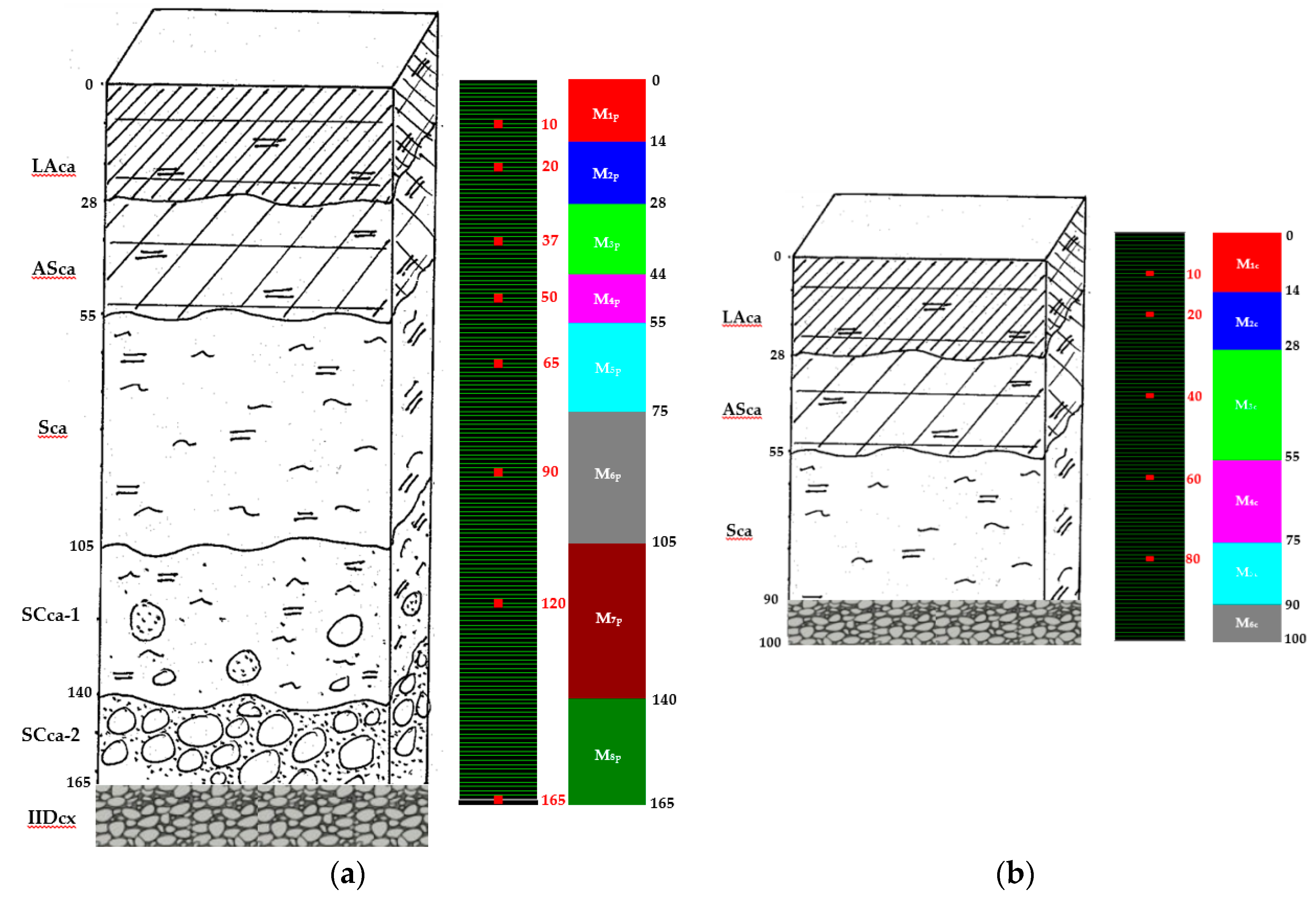
Exposed to a semi-continental climate and the Foehn effect, Colmar is one of the towns in France that receive the lowest rainfall with an annual precipitation average of less than 550 mm as measured between 1986 and 2015. The soil is a Calcaric Cambisol [22] or CALCOSOL derived from loess on Fecht sand/gravel alluvium, according to the French Pedological Referential [23] (Figure 1). The soil is 165 cm thick and consists of five silty loamy horizons, where the clay content slightly decreases with depth (Table S1). The IIDcx horizon found below the soil profile corresponds to recent stony alluvium of the Fecht River.

2.2. Field plots

Three 90 m² (9 × 10 m) bare soil field plots dating from 2000 have been instrumented since January 2013 with T4e tensiometers (UMS GmbH, Frankfurt am Main) and TDR CS605 probes (Campbell Scientific, Logan, UT) placed at eight depths: 10, 20, 37, 50, 65, 90, 120 and 165 cm. Calibration of the TDR probes was based on eleven gravimetric water content profiles measured between September 2013 and February 2015 (data not shown). Soil samples were taken from the same depths at the time of instrumentation for measuring (i) bulk density (ρ_b) using cylinders of 50, 250 and 500 cm³ [24], (ii) water retention (θ(h)) using cylinders of 50 cm³ and the Richards press method [25], (iii) saturated hydraulic conductivity ($K_s$) only for Field Plot 3 using cylinders of 250 cm³ and the constant head method [26].

Bromide ions were added to the surface of each field plot on 18 February 2013 as a KBr solution at 12.5 g Br⁻ L⁻¹ The solution was pulverized using a 9 m ramp at a dose of 4 L m⁻² equivalent to 50 g Br⁻ m⁻². The transport of bromide ions was then studied based on four sample collection rounds (noted C₁ to C₄), which were carried out 112, 279, 526 and 699 days after ploughing. Ploughing was performed on 22 February 2013 using a moldboard plough. Eleven profiles were measured in each round, separated by 0.5 to 1 m along a line perpendicular to the major axis of the plot. Each profile was sampled every 10 cm depth from 0 to 160 cm (0 to 120 cm for C₁). Eight of the profiles were sampled using a motor-driven sample collector (MCL3, GEONOR Inc., Augusta, NJ—section 2.6 cm²) from 0 to 120 cm and then completed from 120 to 160 cm using an auger (section 3.8 cm²) enlarging the hole made by the corer. After C₂, three additional profiles were sampled manually at every 10 cm from 0 to 160 cm, using a large-section auger (17.4 cm²). Bromide was extracted from the samples in the laboratory, using demineralized water, by shaking for one hour at 30 rpm. The bromide concentration was then measured in the supernatant by ionic chromatography using a Compact CI 882 Plus chain (Metrohm France SAS) according to the norm NF EN ISO 10304-1.

2.3. Lysimeters

Six lysimeters were reconstituted in 1983 from soil collected approximately 500 m away from the studied field plots. They are made of 4 m³ (2 × 2 × 1 m) black plastic containers with the bottom slightly inclined toward the center to facilitate water outflow and collection through a drainage hole placed in the middle. The bottom 10 cm consisted of coarse sand to facilitate drainage. When the lysimeters were put in place, the same soil granulometric, physical and chemical properties as those determined for the field plots were obtained. Many studies have been carried out on the six cultivated lysimeters since 1984 (e.g., leaching of nitrates and atrazine, preferential transport of pesticides) with different crop rotation between Lys. 1, 2 and 3 and Lys. 4, 5 and 6. The six lysimeters have been held in bare soil since 2008 and Lys. 1 was instrumented with TDR TRASE probes (Soil Moisture Equipment Corp., Santa Barbara, CA) in March 2009, and with T4e tensiometers in August 2011. Lys. 4 was equipped with TDR CS605 probes in August 2013. The instruments were inserted to the depths of 10, 20, 40, 60 and 80 cm. Tipping-counters (VKWA 100,UGT GmbH, Müncheberg) were installed in late March 2013 at the bottom of each lysimeter to ensure precise measurement of the water outflow over time.

Bromide was added on 20 February 2013 at the same dose as that applied to the field plots (50 g Br⁻ m⁻²) using a movable, electric motor-powered, variable-speed irrigation ramp. Soil tillage was carried out immediately after application using a rotary drill to the depth of 10 cm. The transport of bromide ions was monitored over 127 samples taken from each lysimeter outflow over a period of almost two years (20 February 2013–5 February 2015). Bromide ion content in outflow samples was measured using ion chromatography as in the samples taken from the field plots.

2.4. Climate Data

The climate data used for this study were provided by a meteorological station installed near the experimental center in August 1985. The temperature and humidity of the air, the rainfall, wind speed, and total solar radiation are measured at hourly intervals. A reference daily evapotranspiration value (ET₀) was calculated based on these measurements using the Penman-Monteith equation [27]. Based on ET₀, the maximum daily evaporation of bare soil (E_BS) was estimated using a crop coefficient calculated monthly based on the FAO-56 method [28]. This potential evaporation value produces a satisfactory estimate for the daily value of E_BS with a precision of ±15% according to the literature [29].

2.5. Modelling

2.5.1. Presentation of the Model

Water and bromide transport in soil was simulated using HYDRUS-1D [30]. The mono-dimensional vertical movement of water in the vadose zone is described by the Richards equation [31]:

$$\frac{\partial \theta }{\partial t}=\frac{\partial }{\partial z}\left[K\left(\frac{\partial h}{\partial z}+1\right)\right]$$

(1)

with θ the soil volumetric water content (cm³ cm⁻³), t the time (d), z the coordinate along the vertical axis pointing negatively downwards (cm), h the soil matric head (cm) and K the hydraulic conductivity (cm d⁻¹).

Solving the Richards equation requires the knowledge of two non-linear functions of matric head that describe the soil hydraulic properties, namely the water retention curve θ(h) and the hydraulic conductivity curve K(h). To describe the soil water retention curve, van Genuchten’s expression was used [32] given by:

$$\begin{array}{c}\theta \left(h\right)=\{\begin{array}{cc}{\theta }_r+\frac{{\theta }_s-{\theta }_r}{{\left[1+{\left|\alpha h\right|}^n\right]}^m}& h<0\\ {\theta }_s& h\ge 0\end{array}\\ \mathrm{with}m=1-\frac{1}{n}n>1\end{array}$$

(2)

with ${\theta }_r$ et ${\theta }_s$ respectively the residual and saturated volumetric water content (cm³ cm⁻³), α, an empirical parameter related to the matric head at the inflection point of the retention curve (cm⁻¹) and n, a pore size distribution parameter (-) which determines the slope of the curve at the inflection point.

This expression was associated with the statistical soil pore connection model established by Mualem [33] to predict the hydraulic conductivity function from the water retention curve θ(h). Its application to the van Genuchten model gives:

$$\begin{array}{c}K\left(h\right)=K_s{S}_e^l{\left[1-{(1-S_e{}^{\frac{1}{m}})}^m\right]}^2\\ \mathrm{with}{S}_e=\frac{\theta -{\theta }_r}{{\theta }_s-{\theta }_r}\end{array}$$

(3)

with $K_s$ the saturated hydraulic conductivity (cm d⁻¹), $S_e$, the effective saturation (-) and l, a pore connectivity parameter (-). The latter is most often kept constant regardless of soil type and fixed at 0.5 [33].

HYDRUS-1D also simulates solute transport in the soil using the convection-dispersion equation (CDE) given by:

$$\frac{\partial \left(\theta C\right)}{\partial t}=\frac{\partial }{\partial z}\left(\theta D\frac{\partial C}{\partial z}\right)-\frac{\partial \left(qC\right)}{\partial z}$$

(4)

with C, the solute concentration in liquid phase (g cm⁻³), q, the water flux density (cm d⁻¹) and D, the hydrodynamic dispersion coefficient (cm² d⁻¹) [34] given by:

$$D=\lambda V+\frac{D_0\tau }{\theta }$$

(5)

with λ, the soil dispersivity (cm), V, the average water velocity in soil pores (cm d⁻¹), $D_0$, the solute molecular diffusion coefficient in pure water (1.584 cm² d⁻¹ for bromide) and τ, a tortuosity factor in liquid phase (-) [35] given by:

$$\tau =\frac{{\theta }^{10/3}}{{\theta }_s^2}$$

(6)

Bromide transport in the lysimeters was described by using the dual porosity mobile-immobile water (MIM) model [36]. The MIM model assumes that water movement only takes place in the macroporosity, while the water contained in the microporosity does not participate in the flow, giving the water content and the matric head according to:

$$\theta ={\theta }_m+{\theta }_{im}\mathrm{and}h=h_m=h_{im}$$

(7)

with ${\theta }_m$, the mobile water content (cm³ cm⁻³), ${\theta }_{im}$, the immobile water content (cm³ cm⁻³), $h_m$, the matric head in the mobile region (cm) and $h_{im}$, the matric head in the immobile region (cm).

Therefore, the soil is composed of a mobile region where solute transport is governed by the convection-dispersion equation, and an immobile region where solute transport is only diffusive. Solute can be exchanged between the two regions. Its transport can be modelled according to:

$$\begin{array}{c}\frac{\partial \left({\theta }_m{C}_m\right)}{\partial t}=\frac{\partial }{\partial z}\left({\theta }_m{D}_m\frac{\partial C_m}{\partial z}\right)-q\frac{\partial C_m}{\partial z}-{\alpha }_{ph}\left(C_m-C_{im}\right)\\ \mathrm{and}\frac{\partial {\theta }_{im}{C}_{im}}{\partial t}={\alpha }_{ph}\left(C_m-C_{im}\right)\end{array}$$

(8)

with the m and im indices which respectively designate the mobile and immobile regions and ${\alpha }_{ph}$, the mass transfer coefficient of solute between mobile and immobile regions (d⁻¹).

2.5.2. Representation of the Soil Profiles in HYDRUS-1D

As recommended by Jacques et al. (2002) [37], a soil profile with several layers was defined with a unique soil material associated with each instrumented depth. The soil profiles were very similar between the plots and among the lysimeters. Thus, a unique 165 cm deep profile composed of eight soil materials was created for each plot, while the 100 cm deep profile of each lysimeter comprised six soil materials (Figure 1). Both profiles were vertically discretized using a 1-cm regular mesh size.

2.5.3. Initial and Boundary Conditions

The values provided by the tensiometers at the various instrumented depths were used as the initial matric head profile:

$$h\left(z,t\right)=h_i\left(\mathrm{z}\right)\mathrm{with}t=t_0$$

(9)

with $t_0$ the time of the start of the simulation (d), and $h_i$, the matric head at $t_0$ at depth z (cm).

At the soil surface, a water flux is imposed by the daily maximum bare soil evaporation (E_BS) and rainfall data.

Matric head data acquired by the tensiometer at 165 cm depth were used as the lower boundary condition for each plot:

$$h\left(z,t\right)=h_b\left(t\right)\mathrm{with}z=165$$

(10)

with $h_b$, the matric head measured at 165 cm depth (cm).

For the lysimeters, the bottom boundary condition at 100 cm depth is described by a seepage face condition [21]:

$$\{\begin{array}{ccc}q\left(z,t\right)=0& h<0& z=100\\ h\left(z,t\right)=0& q\ge 0& z=100\end{array}$$

(11)

On the field plots, bromide ions were spread and then buried four days later via a 28 cm-deep ploughing. In the absence of rainfall and with very low potential evaporation observed over the period, bromide at $t_0$ was considered to be uniformly distributed over the last 10 cm of the ploughed LAca layer, i.e., between 18 and 28 cm depth. On the lysimeters, bromide at t₀ was considered to be uniformly distributed over 0–10 cm.

$$\{\begin{array}{lll}C\left(z,t\right)=C_0& t=t_0& 18\le z\le 28\left(0\le z\le 10forlysimeters\right)\\ C\left(z,t\right)=0& t=t_0& 18>z>28(z>10forlysimeters)\end{array}$$

(12)

with $C_0$, the initial bromide ion concentration in soil (g cm⁻³).

For solute transport modelling, a flux condition was imposed on the soil surface:

$$-\theta D\frac{\partial C}{\partial z}+qC=0z=0$$

(13)

while dispersive flux was considered negligible at the lower limit of the soil:

$$\theta D\frac{\partial C}{\partial z}=0z=L$$

(14)

with L, the soil depth (165 cm for the field plots, 100 cm for the lysimeters).

2.5.4. Parameter Optimization Based on the Data Acquired from the Field Plots

For the field plots, model parameters were optimized using the following sequence:

• Initial values were obtained by using the Rosetta software [38] based on the particle size distribution measured for each soil material of each plot, its bulk density as well as its water content measured in the laboratory at −330 and −15,000 cm matric heads.
• These initial values were then used as input for the RetC software [39], which was used to fit the van Genuchten retention curve θ(h) to the measured water retention data. As recommended by Wösten and van Genuchten (1988) [40], the ${\theta }_r$ parameter was not optimized. The simulations based on these RetC parameters will be identified as RP165.
• The values and confidence intervals for parameters ${\theta }_s$, α and n calculated by the RetC software were then used as input in inverse simulations with HYDRUS-1D. Saturated hydraulic conductivity ($K_s$) values obtained from laboratory measurements on Field Plot 3 were used to calculate initial values and confidence intervals for all field plots. The simulations based on these HYDRUS-1D inversed parameters will be identified as P165.

In order to limit the influence of non-uniqueness of the optimized parameters, which is a recurrent problem in inverse simulation [15,41], a strong effort was made to ensure the empirical elimination of the water content data that were deemed abnormal. Similar work was also conducted on the matric head values since tensiometers could be affected by (i) cavitation occurring when approaching −800 cm [42], (ii) temperature variations between day and night, especially during the warm season and potentially leading to changes in soil hydraulic conductivity and affecting the tensiometer electronics [43], (iii) by water frost in the instrument [44], potentially causing damage to tensiometers inserted from the surface, particularly in the winter season. As a result of this work [45] and as recommended by other authors, accurate daily values of (i) matric head, [1,46,47], and (ii) water content were obtained for each instrumented soil material, particularly at low matric head [48,49]. Finally, the parameters were optimized using instrumental data gathered over a period of almost two years (22 February 2013–31 January 2015), consisting of 3200 to 3800 daily values for matric head and water content collected at the various instrumented depths in each plot. Parameter optimization was based on the minimization of a target function, using the Levenberg-Marquardt method [50]:

$$\mathsf{\Phi }\left(b\right)={\displaystyle \sum }_{j=1}^{m_{}}{v}_j{\displaystyle \sum }_{i=1}^{n_j}{w}_{i,j}{\left[x_j^{\ast }\left(z,t_i\right)-x_j\left(z,t_i,b\right)\right]}^2$$

(15)

where $\mathsf{\Phi }$ is the target function, $x_j^{\ast }\left(z,t_i\right)$, the jth variable observed at time $t_i$ at depth z, $x_j(z,t_i,b$) the j^th variable computed with the vector b of parameters (${\theta }_r$, ${\theta }_s$, α, n, $K_s$), m the number of variables measured, $n_j$ the number of measurements for variable j, and finally $v_j$ and $w_{i,j}$ the weights associated with the measured variable j and with each individual value i of variable j. These weights were set to 1 since data are automatically rendered dimensionless by HYDRUS-1D.

The optimization consisted of several successive phases of adjustment of the parameters ${\theta }_r$, ${\theta }_s$,α, n and $K_s$ using the inverse simulation method, one soil material after another starting from the deepest to the one nearest to the surface [51,52]. Once the first round of optimization was completed, the values obtained for ${\theta }_r$ were fixed for the remaining optimization steps. During the second round of optimization, the values of the parameters with high standard errors were replaced by those calculated by RetC (i.e., back to the initial values) and fixed. The third round consisted of extending the limit of the confidence intervals for those parameters which had been placed at the limit, as a result of optimization, upon completion of the first two phases. Finally, during the fourth round, when a correlation higher than 90% was noted between two optimized parameters, the value of one of them was replaced by the value obtained in the previous phase and fixed. In total, more than sixty inverse simulations were carried out for each plot. Finally, concerning the modelling of bromide transport, the dispersivity value (λ) was set manually for each individual horizon in order to obtain the best possible simulation of bromide concentrations based on measured data.

2.5.5. Parameter Optimization Based on the Data Acquired from the Lysimeters

The impossibility of sampling the soil from the lysimeters prevented the measurement of the water retention curve of the soil in the laboratory. The lysimeters were reconstituted from a soil that was similar to the field plots, and the initial values and confidence intervals obtained with RetC based on the samples taken from the field plots were used. The values and confidence intervals of $K_s$ obtained from measurements on Field Plot 3 were also used. The parameters of the coarse sand material situated at the bottom of the lysimeters were defined based on typical hydraulic data for this type of texture [53]. The same optimization principle as the one used for the field plots was used on Lys. 1, using the daily data for matric head, water content and drainage. The parameters established in this way were then used in the optimization work conducted on Lys. 4. In the absence of tensiometer data in this lysimeter, it was decided to fix parameter values for ${\theta }_r$, α and n and optimize ${\theta }_s$ and $K_s$ for the soil materials whose depth had been instrumented with TDR probes (Figure 1). Finally, ${\theta }_s$ and $K_s$ were manually optimized for the non-instrumented Lys. 2, 3, 5 and 6, based on the average values of daily drainage and the confidence interval limits set for ${\theta }_s$ and $K_s$ for Lys. 1 and 4. The data gathered on lysimeters covered approximately two years (20 February 2013–28 February 2015) and included (i) 3186 values of matric head for Lys. 1, (ii) 1521 and 2845 water content values respectively, for Lys. 1 and 4, (iii) 707 drainage values collected from each of the six lysimeters. The simulations based on these HYDRUS-1D inversed parameters will be identified as L.

2.5.6. Cross Simulations

Cross simulations were carried out between the field plots and the lysimeters in order to ascertain to what extent the optimized parameters for the lysimeters could be used to simulate the water dynamics and solute transport processes in the field plots, and vice versa. With this in mind, a 90 cm deep profile was considered for each field plot to ensure that the depth of the profile was identical to that of lysimeters. Three horizons (LAca, ASca and Sca) and six soil materials (M_1p to M_6p) were consequently taken into account (Figure 1). The matric head data measured by the tensiometer located at 90 cm was used as the lower boundary condition. The simulation consisted in applying the mean values of the optimized parameters found for each soil material of all lysimeters to the corresponding soil materials of each field plot and comparing the result of the simulation to the water and bromide data obtained in the field plots (simulations noted L*). Similarly, the parameters estimated using field plot data were applied to simulate the lysimeter experiments (P* simulations).

2.6. Evaluation of Simulation Quality

The quality of the simulations was evaluated based on the efficiency coefficient (E) [54].

$$E=1-\frac{{\sum }_{i=1}^n{(x_o^t-x_m^t)}^2}{{\sum }_{i=1}^n{(x_o^t-\overline{x_o})}^2}$$

(16)

where $x_o^t$ is the data observed at time t, $x_m^t$ the data modelled at time t and $\overline{x_o}$ the average value of the observed data.

Efficiency coefficients were calculated based on daily values of matric head, water content and lysimeter outflow as well as bromide concentrations determined on the soil samples taken from the field plots or on the water samples collected from the lysimeters.

3. Results and Discussion

3.1. Measurements

3.1.1. Soil Physical Characteristics

The particle size fractions were similar in horizons ASca, Sca and SCca-1 in the three field plots with a slightly lower clay content and higher silt content with increasing depth (Figure 1, Table S1). Despite some disparities between the field plots (clay and silt content in LAca and sand content in SCca-2), all horizons presented the same texture according to the USDA classification (silty loam). In view of the small differences in bulk density associated with a coefficient of variation of less than 9.5%, it was assumed that bulk density was identical in all plots at each single depth (Table S2). This value was calculated as the average of all values obtained from samples collected at the given depth from all three field plots. The coefficient of variation of the saturated hydraulic conductivity was less than 71% (Table S2), which is consistent with the observations made by other authors [55].

Concerning the lysimeters, the proportions of clay, silt and sand, as well as the bulk density were not very different from the average values obtained for the field plots (

Table 1. Particle size distribution and bulk density of the field plots and lysimeters. When available, standard deviations are reported in parentheses.

Layer (cm)	Field Plots (2012)				Lysimeters (1983)
	Clay	Silt	Sand	ρb	Clay	Silt	Sand	ρb
	(%)			(g cm−3)	(%)			(g cm−3)
0–30	23.6 (0.7)	65.9 (0.8)	10.5 (0.9)	1.38 (0.11)	23.9	69.2	6.9	1.34
30–60	23.7 (1.7)	66.0 (0.9)	10.3 (1.2)	1.25 (0.07)	23.3	70.4	6.4	1.22
60–90	16.4 (1.7)	68.6 (1.5)	15.0 (1.3)	1.41 (0.08)	17.5	72.3	10.3	1.37

) since similar soil samples were used for the construction of the lysimeters in 1983.

3.1.2. Water Dynamics

The variations in matric head and water content measured at the same depth in the three field plots are relatively similar and, as expected, influenced by the alternation between rain and evaporation over time, particularly from the surface down to 40 cm depth (Figure S1). The effects of a drier spring and summer in 2014 can be seen down to 90 cm depth. Matric head and water content dynamics observed in the winter of 2013–2014 and 2014–2015 are comparable.

The water content dynamics observed in Lys. 1 and 4 are comparable, despite a certain gap, which remained constant over time, at the depths of 40 and 60 cm (Figure 2 and Figure S2). This gap can be attributed to the lack of calibration of the TDR probes installed in the lysimeters [56,57], or differences in the structure and porosity of the soil, which could have been produced during the construction of the lysimeters [58]. However, the latter explanation is less probable than the former because no difference in bulk density was observed between the lysimeters and the field plots. Between 496 (Lys. 4) and 559 mm (Lys. 2) of water were recovered from the lysimeters between 25 March 2013 and 28 February 2015 (Figure 3 and Figure S3), which amount to 41 to 47% of the total rainfall observed during that period (1194 mm). A similar trend was noted for Lys. 1, 2 and 3 and Lys. 4, 5 and 6, with Lys. 1, 2 and 3 producing higher outflow after heavy rainfalls (e.g., October 2013, July 2014), which made a difference of approximately 20 mm y⁻¹ compared to the other three lysimeters. This could be caused by the reconstitution of the lysimeters, as well as by different crop rotation conducted since their installation in 1983 and until 2007.

Only the hydraulic heads and water contents observed in the LAca horizon (0–28 cm) of the field plots and lysimeters presented overlapping standard deviations (Figure 2). The average moisture content was higher in the lysimeters than in the field plots below the LAca horizon in Lys. 1 and below 40 cm depth in Lys. 4. The hydraulic head profile in Lys. 1 was close to saturation below 20 cm depth regardless of the season, which is typical for lysimeters kept under bare soil with an atmospheric lower boundary condition. It was shown already that lysimeters disturb the natural soil water dynamics, with the intensity of the disturbance being dependent on the lysimeter depth [59,60].

3.1.3. Bromide Transport

The experimental bromide transport is described in supplementary Figure S4 for the field plots and in supplementary Figure S5 for the lysimeters.

Bromide concentration profiles were similar for the three field plots. The only difference was in the peak value, which was lower in Field Plot 2 at C₁ (13 June 2013) and in Field Plot 3 at C₂ (27 November 2013), resulting in less accurate mass balances. The quantity of bromide leached out of the soil profile was negligible at C₁ and C₂, whilst approximately 10 g m⁻² were leached on 1 August 2014 (C₃), and even more at C₄. The downward movement of bromide was the result of net infiltrations of 56 to 150 mm between each round of measurements, and mainly depended on daily rainfalls exceeding 10 mm. The number of these infiltrations varied between 8 and 13 and accounted for 40 to 56% of the total rainfall measured during each period.

The first traces of bromide in the lysimeter outflows were collected after the summer of 2013, when outflows started again. This corresponds to approximately 200 days and 90 mm of outflow after bromide application (Figure S5). On the last day of collection (5 February 2015), i.e., 715 days after the application and for cumulative outflows between 493 (Lys. 4) and 556 mm (Lys. 2), no bromide was detectable anymore in the lysimeter outflows. Peak concentrations varied between 272 and 358 mg L⁻¹ for a cumulative outflow of 196 to 241 mm. These water amounts are at least 16% lower than the water retention capacity measured in the lysimeters, which was estimated at 287 mm based on neutron probe measurements made in 2001. This would mean that some of the water contained in the lysimeters did not participate in the transport of bromide and that preferential flow [61,62] occurred. Several processes already reported in the literature could explain the preferential transport of bromide in the lysimeters, such as (i) the soil disturbance that may have induced differences in soil structure and porosity compared to the undisturbed soil of the field plots, at least for some time [63]; (ii) the modification of the soil water dynamics, induced by the rupture of capillarity at the bottom of the lysimeter [21]; (iii) the water content close to saturation [64] observed at 40 cm and deeper; (iv) the interruptions of drainage [12].

Bromide concentration time series were found to be relatively similar between all lysimeters (Figure S5), presenting only small differences depending mainly on the amount of cumulated outflow related to the lysimeter position. The total quantity of bromide collected in the outflow of the lysimeters ranged from 34 to 45 g m⁻², which represented between 69 and 89% of the application (50 g m⁻²).

3.2. Modelling

The figures and tables relative to the simulations made on Field Plot 1 and Lys. 1 are presented in the main text. The figures and tables relative to the simulations made on Field Plots 2 and 3 and Lys. 2, 3, 4, 5 and 6 are given as supplementary material.

3.2.1. Field Plots

The van Genuchten parameters (${\theta }_r$, ${\theta }_s$ α and n) obtained with RetC based on the laboratory results were relatively similar for the same soil material in the three field plots (Figure S6,

Table 2. Parameters optimized using HYDRUS-1D for each of the eight soil materials of Field Plot 1.

Soil Material	${\mathit{\theta }}_{\mathit{r}}$	${\mathit{\theta }}_{\mathit{s}}$	α	n	${\mathit{K}}_{\mathit{s}}$	λ	${\mathit{\theta }}_{\mathit{s}}\ast$
	cm3 cm−3		cm−1	-	cm d−1	cm	cm3 cm−3
M1p	0.066 (0.073) [0.066–0.076]	0.364 (0.411) [0.359–0.368]	0.021 (0.054) [0.020–0.023]	1.252 (1.162) [1.240–1.264]	101.2	4.0	0.329 [0.327–0.330]
M2p	0.076 (0.077) [0.076–0.079]	0.381 (0.439) [0.370–0.391]	0.077 (0.196) [0.067–0.087]	1.144 (1.139) [1.133–1.155]	776.8 [571.4–982.2]	4.0	0.317 [0.316–0.319]
M3p	0.075 (0.076) [0.075–0.080]	0.373 (0.420) [0.370–0.376]	0.036 (0.028) [0.034–0.038]	1.181 (1.162) [1.161–1.200]	45.6	4.0	0.325 [0.323–0.327]
M4p	0.065 (0.068) [0.065–0.070]	0.313 (0.448) [0.295–0.330]	0.007 (0.076) [0.001–0.012]	1.364 (1.183) [1.343–1.384]	76.9	4.0	0.299 [0.297–0.301]
M5p	0.046 (0.048) [0.046–0.051]	0.320 (0.412) [0.306–0.335]	0.017 (0.043) [0.012–0.021]	1.158 (1.204) [1.116–1.200]	27.1 [7.9–46.3]	1.5	0.302 [0.300–0.304]
M6p	0.050 (0.051) [0.050–0.055]	0.327 (0.395) [0.322–0.332]	0.004 (0.007) [0.002–0.006]	1.654 (1.279) [1.442–1.867]	16.7	1.5	0.315 [0.313–0.317]
M7p	0.041 (0.044) [0.041–0.047]	0.351 (0.394) [0.342–0.360]	0.002 (0.005) [0.002–0.002]	1.452 (1.452)	16.1	3.0	/
M8p	0.040 (0.037) [0.036–0.040]	0.390 (0.311) [0.382–0.398]	0.006 (0.002) [0.006–0.006]	1.463 (1.463)	19.8	3.0	/

Note: Initial values obtained with RetC from laboratory water retention measurements are given in parentheses after the optimized value. Confidence intervals associated with parameters optimized using HYDRUS-1D are given in brackets. Parameters ${\theta }_r$, α, n and $K_s$ optimized using HYDRUS-1D are highlighted: (i) in bold for parameters whose optimized value is not included in the initial bounds, (ii) in italics for non-optimized parameters set to the mean initial value. Saturated water content values re-optimized during the cross-simulations are noted ${\theta }_s$*. The soil dispersivity (λ) was set manually for each individual soil material.

and Table S3). The values of parameters ${\theta }_r$, ${\theta }_s$ and α were generally higher for horizons LAca and ASca (M_1p to M_4p) than those for horizons SCa and SCca (M_5p to M_8p) whilst the opposite was found for parameter n. However, these parameters did not allow to describe the water dynamics observed in situ in a satisfactory manner (RP165 in Figure 4 and Figure S7 and

Table 3. Efficiency coefficients calculated at each instrumented depth in Field Plot 1 and based on different optimization procedures using HYDRUS-1D. RP165 for results obtained with the parameters optimized with RetC, P165 for results obtained with the parameters optimized with HYDRUS-1D on the 165 cm deep profile; P90 for results obtained by applying the parameters optimized for the 165 cm deep profile to the 90 cm deep profile; L* for results obtained by applying the mean optimized parameters from the six lysimeters; oL*, the same as L* but for saturated water content values (${\theta }_s$*) again optimized for each soil material.

Simulation	M1p_10	M2p_20	M3p_37	M4p_50	M5p_65	M6p_90	M7p_120	M8p_165
h_RP165	0.21	0.06	−0.71	−1.26	−0.81	0.86	0.86	1.00
h_P165	0.48	0.47	0.72	0.78	0.79	0.88	0.87	1.00
h_P90	0.49	0.46	0.69	0.83	0.78	1.00	/	/
h_L*	0.41	0.43	0.48	0.63	0.76	1.00	/	/
h_oL*	0.48	0.44	0.51	0.66	0.76	1.00	/	/
θ_RP165	−1.39	−1.76	−9.92	−17.73	−22.48	−35.59	−13.52	−19.88
θ_P165	0.65	0.58	0.64	0.71	0.84	0.73	0.67	0.83
θ_P90	0.67	0.61	0.71	0.81	0.80	0.44	/	/
θ_L*	0.21	−0.31	−0.76	−7.35	−133.53	−69.30	/	/
θ_oL*	0.62	0.30	0.38	0.39	0.84	0.80	/	/

and Table S4).

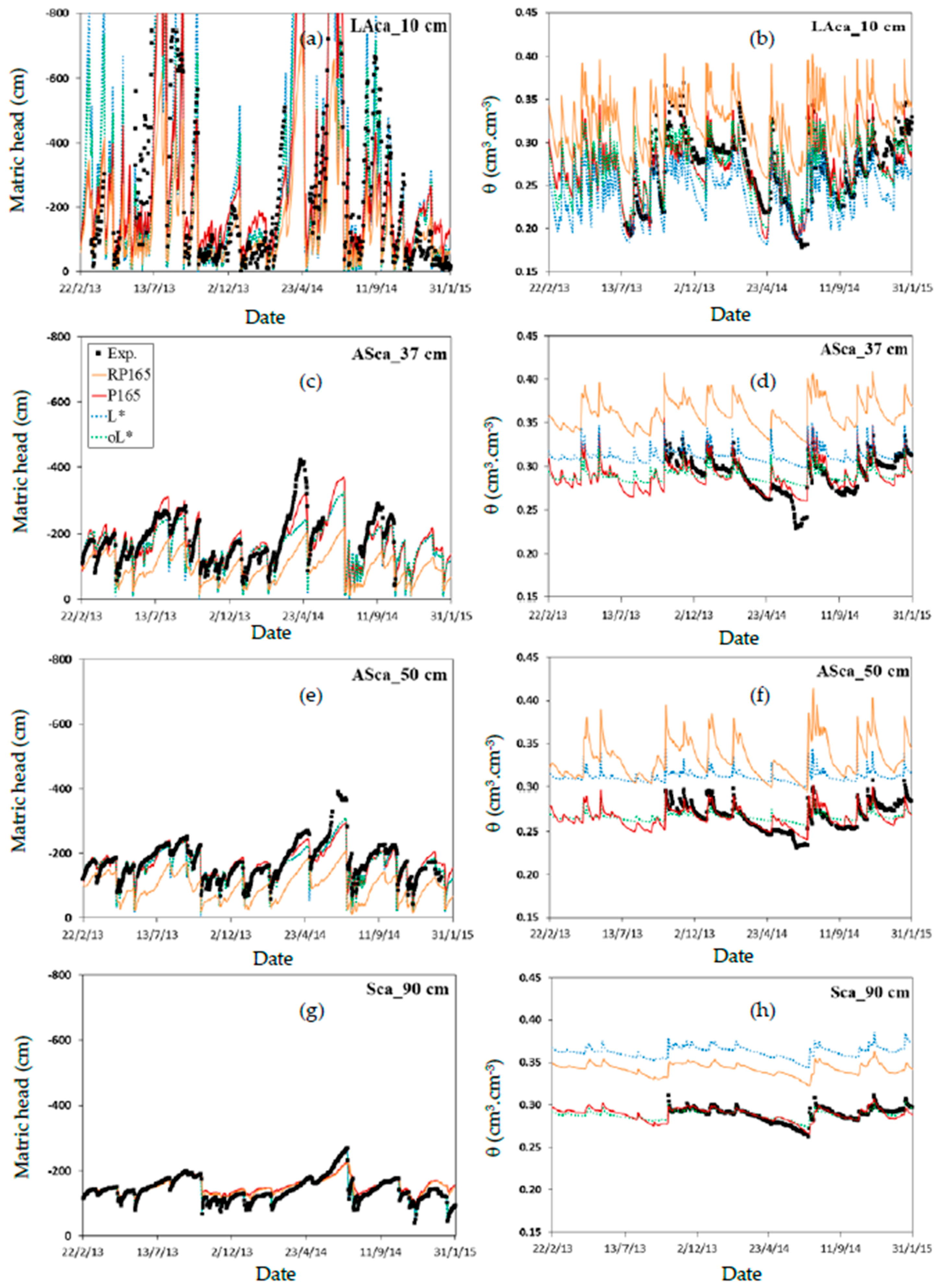
After the parameters optimization carried out with HYDRUS-1D, a satisfactory description of the experimental data measured at depths below the tilled layer was obtained (P165 in Figure 4 and Figure S7) with efficiency coefficients mostly higher than 0.7 for matric head data and 0.6 for water content data (P165 in Table 3 and Table S4). The lower E values found in the surface horizon (LAca) may be due to (i) the temporal variability of the physical and hydraulic properties of the LAca horizon due to the tillage operations [65]; (ii) the effect of withdrawal and re-installation of the tensiometers and TDR probes with every tillage operation. A general over-estimation of matric head and water content by the model was observed when the soil was dry and, inversely, an under-estimation for wet soil, particularly for the topsoil down to 37 cm (P165 in Figure 4 and Figure S7). Several optimized parameters were not included in the intervals initially set using RetC, notably ${\theta }_s$, which generally fell below the minimum limit (Table 2 and Table S3). This confirms the general finding that laboratory measurements overestimate field saturated water contents [66,67]. More generally, the low efficiency coefficients found when using the laboratory derived hydraulic parameter values (RP165 in in Table 3 and Table S4) confirm that these values are not representative of field soil, supporting the conclusions of the studies conducted by other authors [68,69]. The values of the parameters optimized with HYDRUS-1D show the same evolution with depth as the values obtained using RetC with ${\theta }_r$, α and $K_s$ values generally lower at greater depths, whilst the opposite is noted for n (Table 2 and Table S3). Values of optimized parameters on the three field plots are usually close for the same soil material (except α for M_2p, n for M_5p and M_6p and $K_s$ for M_3p, Table 2 and Table S3) which is not the case for the soil materials within the same layer. This emphasizes the importance of defining as many soil materials as instrumented depths [37]. Confidence intervals associated with each optimized parameter are relatively small around the optimized value.

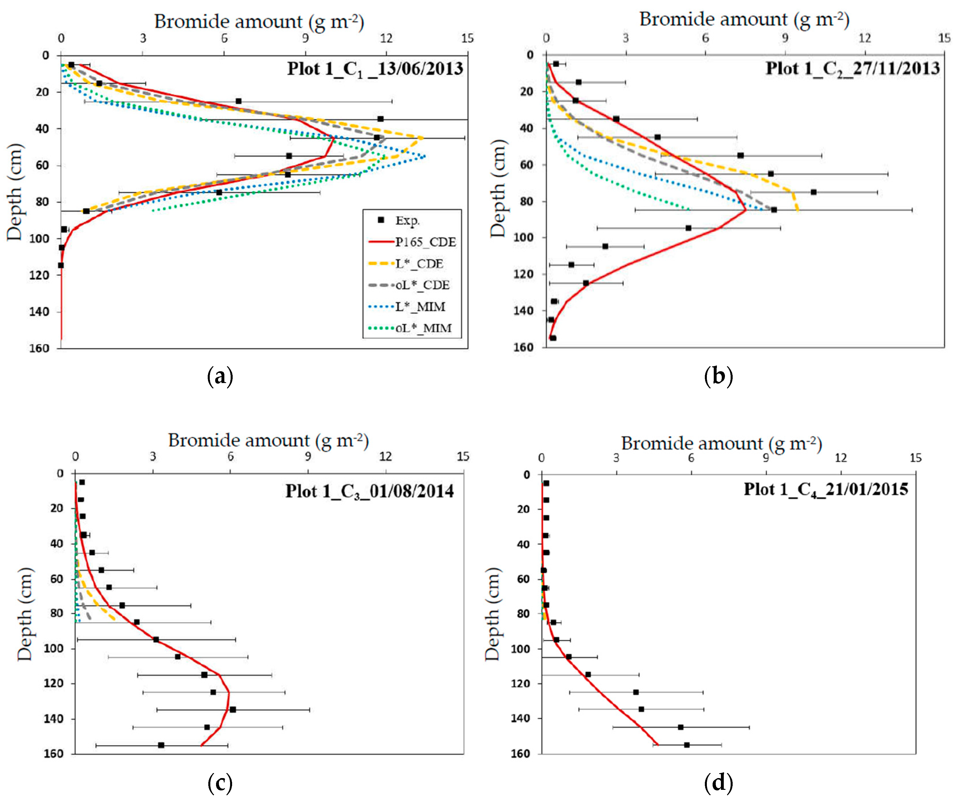
As shown by Figure 5 and Figure S8, the transport of bromide was correctly simulated in each field plot by the convection-dispersion model using the optimized hydraulic parameters (P165_CDE). Dispersivity values were calibrated manually for individual horizons (Table 2 and Table S3). These values remain within the range found for field experiments with soils of similar texture [70]. The efficiency coefficients obtained range from 0.53 to 0.95 and are often higher than 0.70 (P165_CDE in

Table 4. Efficiency coefficients calculated for bromide transport for each monitoring campaign (C₁ to C₄) conducted on Field Plot 1 and based on different optimization procedures using HYDRUS-1D.

Simulation	C1 (13 June 2013)	C2 (27 November 2013)	C3 (1 August 2014)	C4 (21 January 2015)
P165_CDE	0.93	0.80	0.93	0.89
P90_CDE	0.87	0.82	0.80	/
L*_CDE	0.74	0.84	0.20	/
oL*_CDE	0.84	0.65	−0.73	/
L*_MIM	0.30	0.11	−1.37	/
oL*_MIM	0.38	−0.47	−1.57	/

Note: P165 for results obtained with optimized parameters with HYDRUS-1D on the 165 cm deep profile; P90 for results obtained by applying the parameters optimized for the 165 cm deep profile to the 90 cm deep profile; L* for results obtained by applying the mean optimized parameters from the six lysimeters; oL*, the same as L* but for saturated water content values (${\theta }_s$*) again optimized for each soil material. CDE for results obtained with the convection-dispersion equation. MIM for results obtained with the mobile-immobile model. Due to a lack of bromide in the 90 cm deep profile, efficiency coefficients were not calculated for the fourth monitoring campaign.

and Table S5). This indicates that the experimental data were reproduced in a satisfactory manner by the model over a period of more than 700 days.

3.2.2. Lysimeters

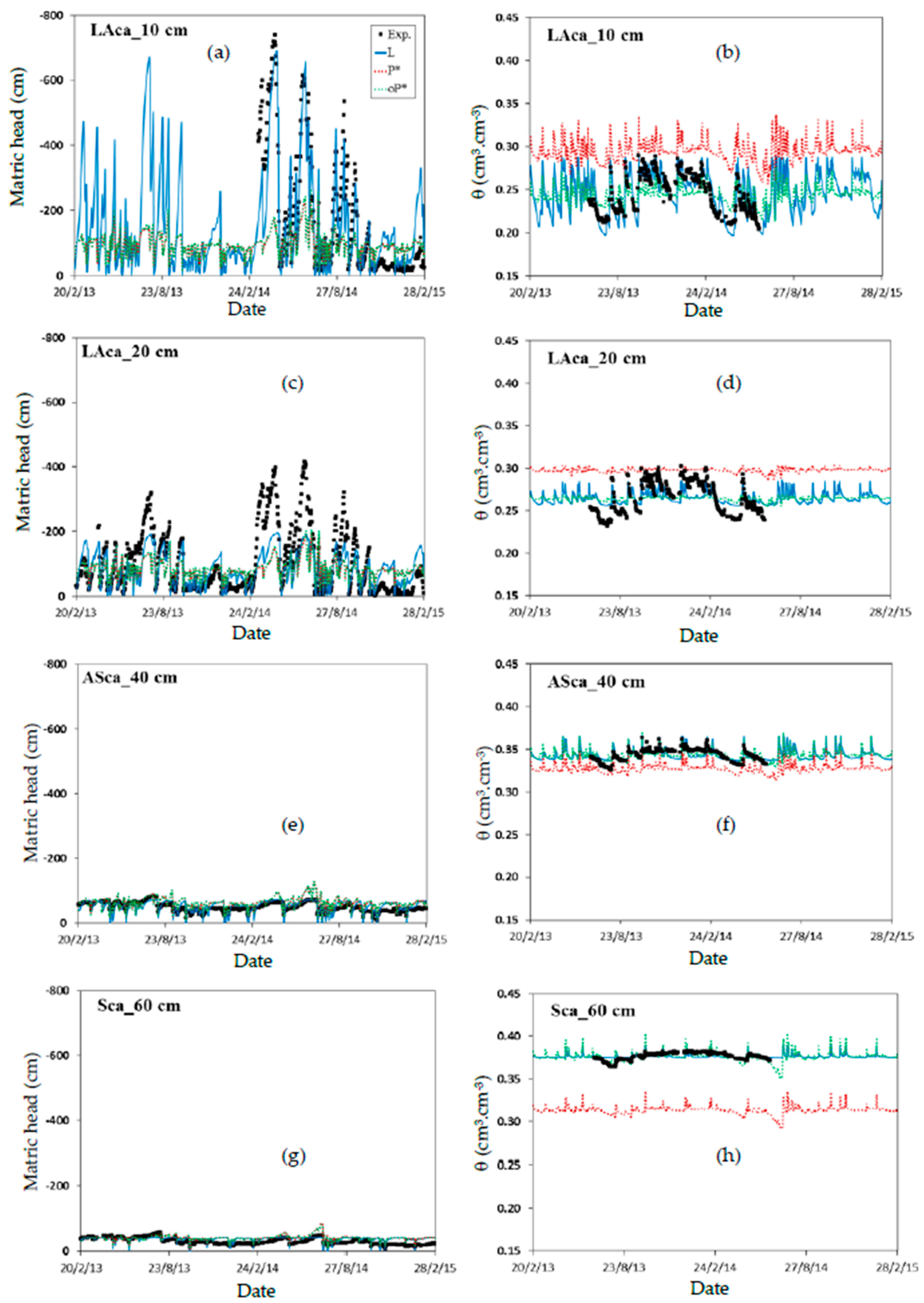
The peculiarity of the soil water regime observed in the lysimeters complicated the optimization and prevented us from producing an accurate simulation of the data measured below the surface horizon (see L in Figure 6 and Figure S9). This was particularly visible at depths of 40 cm and lower, where the small variations in matric head and water content were difficult to simulate precisely (E near or inferior to 0, for h_L and θ_L in

Table 5. Efficiency coefficients calculated for matric head and water content data at each depth instrumented in Lys. 1 using HYDRUS-1D.

Simulation	M1c_10	M2c_20	M3c_40	M4c_60	M5c_80
h_L	0.74	0.54	−0.14	−0.93	−0.07
h_P*	−0.06	0.17	−0.72	−1.59	0.53
h_oP*	−0.06	0.17	−0.80	−1.60	0.54
θ_L	0.62	0.41	0.43	0.07	0.05
θ_P*	−5.69	−1.59	−9.97	−142.89	−165.11
θ_oP*	0.33	0.36	0.36	0.37	0.43

Note: L for results obtained with the parameters optimized with HYDRUS-1D on lysimeter data; P* for results obtained by applying the mean optimized parameters from 165 cm deep profile of the three field plots; oP*, the same as P* but for saturated water content values (${\theta }_s$*) again optimized for each soil material.

and Table S6). As for the field plots, a slight over-estimation of experimental data by the model for dry soil was noted as well as a slight under-estimation for wet soil, both being mainly visible for the topsoil of Lys. 1 and 4 (Figure 6 and Figure S9).

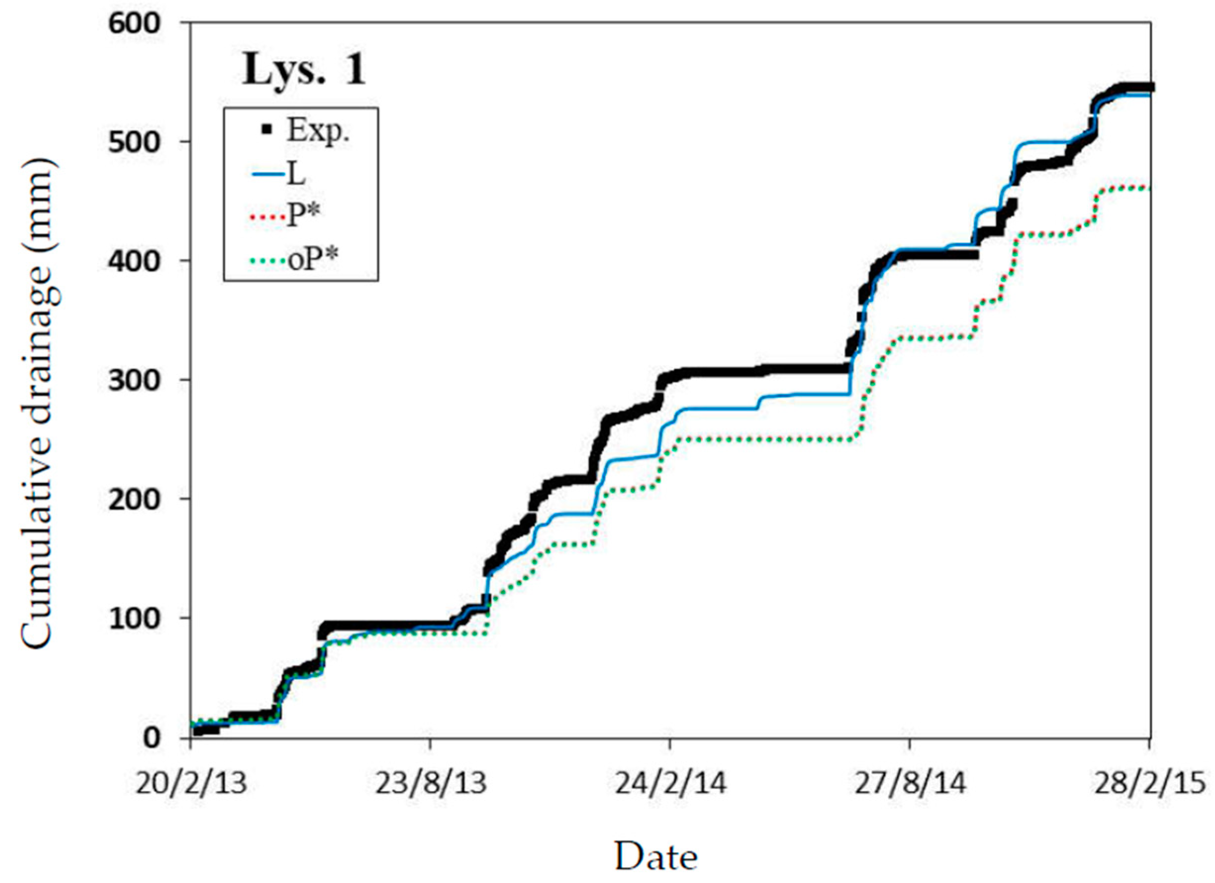
The drainage measured on the six lysimeters over more than two years was simulated relatively well by the model (Figure 3 and Figure S3), with efficiency coefficients exceeding 0.72 (d_L in

Table 6. Efficiency coefficients calculated for daily drainage data on Lys. 1 using HYDRUS-1D.

Simulation	Lys. 1
d_L	0.81
CV	−1.2
d_P*	0.79
CV	−14.7
d_oP*	0.79
CV	−14.9

Note: L for results obtained with the parameters optimized with HYDRUS-1D on lysimeter data; P* for results obtained by applying the mean optimized parameters from 165 cm deep profile of the three field plots; oP*, the same as P* but for saturated water content values (${\theta }_s$*) again optimized for each soil material. Coefficients of variation (CV) were calculated from cumulative experimental and simulated drainage data and are given in %.

and Table S7) and relative gaps between cumulated experimental and simulated drainages, ranging from −2.3 to +0.6% by the end of the modelling period. Data analysis showed that simulated drainage was generally (i) lower than that measured during intense drainage events; (ii) higher than those measured when drainage was low, especially when measured values were smaller than 2 mm per day. Consequently, the under-estimation produced by the model in the winter 2013–2014 (Figure 3 and Figure S3) was compensated by an over-estimation during the summer 2014. The bias relative to the calculation of the maximum evaporation of bare soil (E_BS) based on ET₀ could perhaps explain these differences. Only a few studies have been dedicated to the validation of the estimation of bare soil evaporation [71,72], in spite of the multitude of estimation methods [73]. In the absence of a means of comparison, the same daily values of E_BS were considered for the field plots and for the lysimeters in spite of possible differences generally attributed to different water content profiles [74] and to the limited depth of the lysimeters [75].

After optimization on Lys. 1 data, only the value of parameters α, n and $K_s$ for the second soil material (M_2c) turned out to be different from the other four soil materials (

Table 7. Parameters optimized using HYDRUS-1D for each of the six soil materials of Lys. 1.

Soil Material	${\mathit{\theta }}_{\mathit{r}}$	${\mathit{\theta }}_{\mathit{s}}$	α	n	${\mathit{K}}_{\mathit{s}}$	${\mathit{\theta }}_{\mathit{s}}\ast$
	cm3 cm−3		cm−1	-	cm d−1	cm3 cm−3
M1c	0.062 (0.072) [0.062–0.108]	0.289 (0.402) [0.287–0.291]	0.020 (0.047) [0.020–0.020]	1.194 (1.168) [1.189–1.200]	10.0 (110.2)	0.286 [0.282–0.290]
M2c	0.097 (0.078) [0.069–0.097]	0.288 (0.394) [0.286–0.290]	0.200 (0.084)	1.050 (1.168)	1000.0 (575.2)	0.324 [0.320–0.329]
M3c	0.109 (0.080) [0.065–0.109]	0.366 (0.423) [0.364–0.368]	0.035 (0.055)	1.100 (1.174)	30.0 (73.9)	0.384 [0.380–0.388]
M4c	0.065 (0.075) [0.065–0.095]	0.389 (0.431) [0.387–0.391]	0.012 (0.068)	1.140 (1.181)	15.0 (76.9)	0.410
M5c	0.058 (0.049) [0.043–0.058]	0.396 (0.394) [0.394–0.398]	0.009 (0.021)	1.150 (1.252)	25.0 (22.9)	0.397
M6c	0.010	0.450	0.150	3.000	3000.0	/

Note: Initial parameters are given in parentheses after the optimized value. Confidence intervals associated with parameters optimized using HYDRUS-1D are given in brackets. Parameters ${\theta }_r$, ${\theta }_s$, α, n and $K_s$ optimized using HYDRUS-1D are highlighted: (i) in bold for parameters whose set value is not included in the initial bounds, (ii) in italics for parameters that were set manually. Saturated water content values re-optimized during the cross simulations are noted ${\theta }_s$*.

). Furthermore, given that the soil was continuously close to saturation at 40 cm depth and below, the problem of inversion occurring in lysimeters affected mostly the α, n and $K_s$ parameters, producing very large confidence intervals. Consequently, unlike for the field plots, many parameters (in italics in Table 7) could not be optimized and had to be calibrated manually. The few confidence intervals associated with optimized parameters were small around the optimized value. Finally, few optimized parameters on lysimeters are included in the confidence intervals of those of the field plots and vice versa (Table 2 and Table S3 vs. Table 7 and Table S8).

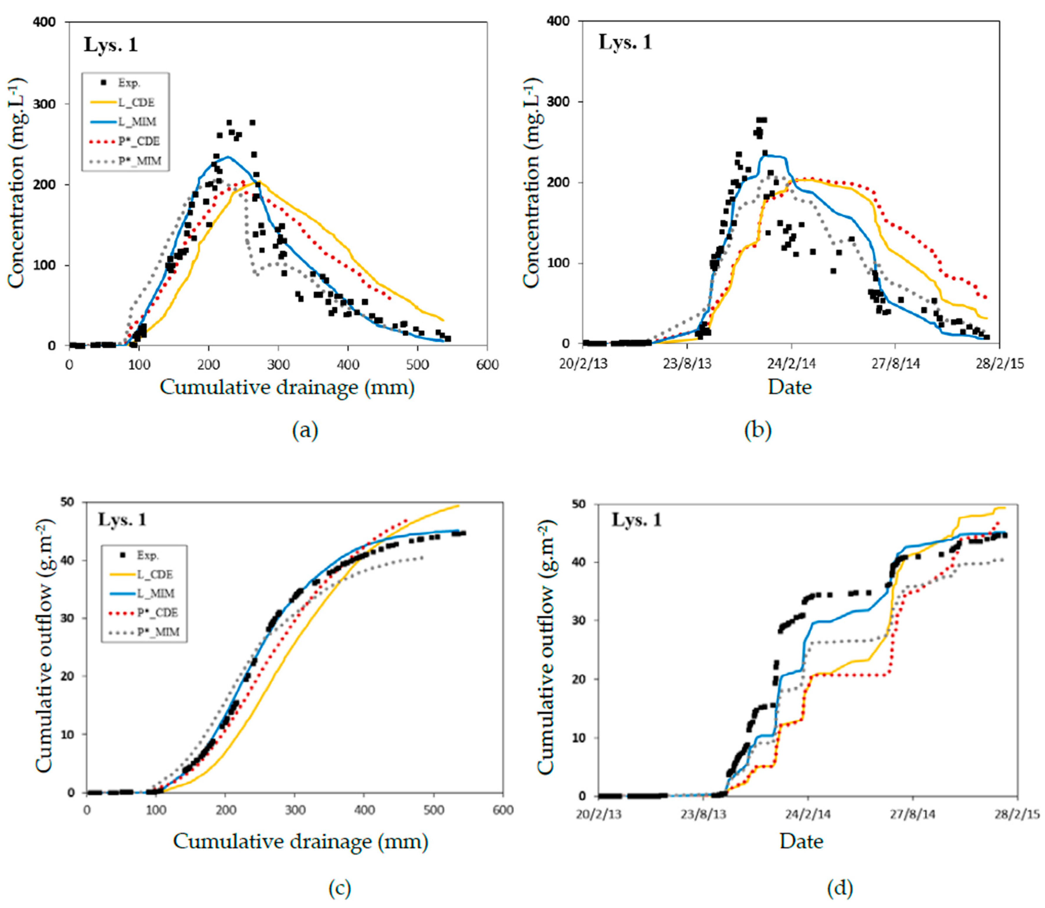
Bromide concentration in the outflow of the six lysimeters could not be adequately modelled based on the convection-dispersion equation (L_CDE in Figure 7 and Figure S10). The simulated displacement of bromide was slower than that observed for all lysimeters. As already highlighted in the literature, bromide transport in lysimeters can be influenced by preferential transport [76], which was modelled here with HYDRUS-1D using its mobile/immobile water module [77]. A unique value of dispersivity, immobile water content and mass transfer coefficient was calibrated manually on all soil materials of the same lysimeter (

Table 8. Values of dispersivity, immobile water content and mass exchange coefficient parameters manually set using HYDRUS-1D for all soil materials of Lys. 1. Initial amounts of bromide manually re-optimized are noted C₀*.

Parameter	Lys. 1
λ [cm]	2.00
${\theta }_{im}$[cm3 cm−3]	0.060
C0* [g m−2]	59.2
${\alpha }_{ph}$[d−1]	10−6

and Table S9), allowing for an adequate simulation of the bromide outflow observed experimentally (L_MIM in Figure 7 and Figure S10).

As a result, the efficiency coefficients were considerably higher than those obtained by the CDE model (

Table 9. Efficiency coefficients calculated for bromide concentration and cumulated outflow as a function of time (and cumulative drainage in parentheses) from Lys. 1 and based on different optimization procedures using HYDRUS-1D.

Variable	Simulation	Lys. 1
Concentration	L_CDE	0.37 (0.61)
	L_MIM	0.83 (0.93)
	P*_CDE	0.34 (0.80)
	P*_MIM	0.84 (0.67)
Cumulated Outflow	L_CDE	0.08 (0.32)
	L_MIM	0.60 (0.63)
	P*_CDE	0.41 (0.39)
	P*_MIM	0.90 (0.18)

Note: L_CDE for results obtained with the convection-dispersion equation and parameters optimized with HYDRUS-1D on lysimeter data; L_MIM for results obtained with the mobile-immobile model and parameters optimized with HYDRUS-1D on lysimeter data; P*_CDE for results obtained with the convection-dispersion equation and by applying the mean optimized parameters from the 165 cm deep profiles of the three field plots; P*_MIM for the results obtained with the mobile-immobile model and by applying the mean optimized parameters from the 165 cm deep profiles of the three field plots.

and Table S10). Simulations provided a better description of bromide outflow when expressed as a function of cumulated drainage rather than as a function of the sampling date (Figure 7 and Figure S10, Table 9 and Table S10). This difference is due to the underestimation of drainage in the summer 2014 and its overestimation in the winter 2013–2014. Furthermore, obtaining a satisfactory simulation for each lysimeter using the MIM model is conditioned by the optimization of the quantity of bromide applied at t₀ (C₀* in Table 8 and Table S9), which is sometimes considerably different from the target quantity (50 g m⁻²). The results indicate a more uniform pulverization for Lys. 4, 5 and 6, which are closer to the target dose.

3.2.3. Cross Simulations

The results obtained for the 90 cm deep profile of the field plots are similar to those obtained for the 165 cm deep profile and are consequently not illustrated in this paper. First, the average parameters optimized on lysimeter data (Table S11) were applied to the field plots down to 90 cm depth using HYDRUS-1D (L* in Figure 4 and Figure S7). Matric head, and especially water content experimental data, were less adequately described than when using the parameters optimized on field plot data (P_165) but often better than when using laboratory-determined parameters (RP165). This is highlighted by a decrease in the value of the efficiency coefficient at all depths (θ_L* in Table 3 and Table S4), particularly for water content data, when compared to the field plot optimized parameters (θ_P90) but also some higher values compared to the initial RetC parameters (θ_RP165). However, once the value of the saturated water content had been optimized again for each soil material (${\theta }_s$* in Table 2 and Table S3), the efficiency coefficients rose considerably for water content, coming close to those obtained with the parameters optimized directly on field plot data (θ_oL* in Table 3 and Table S4). Consequently, the value of ${\theta }_s$ represents the main bias for the transposition of optimized parameters from the lysimeters to the field plots. Another bias concerns the difficulties with which the model simulates soil desiccation at the depth of 20 cm (LAca) to 50 cm (ASca) (L* in Figure 4 and Figure S7). This was mostly due to the fact that at the depth of 20 cm, the water content regime in the lysimeters is intermediate between that observed at the soil surface, and the virtually saturated state found at 40 cm or deeper (Figure 2). Therefore, the majority of parameters α, n and $K_s$ for soil materials 2 to 5 in the lysimeters had to be set manually in HYDRUS-1D (Table 7). The transport of bromide in the field plots was also less well simulated by the MIM model using the average parameters optimized on the lysimeters (λ = 1.1 cm, ${\theta }_{im}$ = 0.073 cm³ cm⁻³ and α_ph = 10⁻⁶ d⁻¹). Indeed, simulated transport was too fast compared to observations whether the ${\theta }_s$ values were optimized again or not (L*_MIM and oL*_MIM in Figure 5 and Figure S8). This results in efficiency coefficients being lower than 0 when pooling all measurement campaigns conducted between June 2013 and August 2014 (L*_MIM and oL*_MIM in Table 4 and Table S5). Nevertheless, a better simulation of bromide transport was obtained when using the CDE model with parameters optimized on lysimeter data (L*_CDE and oL*_CDE in Figure 5 and Figure S8), except for the first sampling dates for Field Plots 2 and 3. In spite of this, the efficiency coefficients obtained were still lower than those calculated based on the parameters optimized on field plot data (L*_CDE and oL*_CDE vs. P90_CDE in Table 4 and Table S5). Consequently, the preferential transport observed in the lysimeters represents an artifact that does not allow an adequate simulation of the solute transport observed experimentally in the field plots, in spite of having their water dynamics adequately simulated once the ${\theta }_s$ values were optimized.

The average parameters optimized on field plot data (Table S12) were then applied to the lysimeters. The drying of the topsoil in Lys. 1 and 4 was not as well simulated as when using the parameters directly optimized on lysimeter data, particularly at 10 cm depth, even when the ${\theta }_s$ values have been optimized again (oP* in Figure 6 and Figure S9). The efficiency coefficients calculated on water content data improved considerably when the ${\theta }_s$ values were reset (oP* in Table 5 and Table S6). The differences in the parameter values α, n and $K_s$ between soil materials 1 and 2 in the lysimeter profile (Table 7) seem to be essential for an adequate simulation of water content and matric head at the depth of 10 cm and 20 cm. Furthermore, in spite of efficiency coefficients being comparable (Table 6 and Table S7), the drainage simulation based on field plot parameters still under-estimated the experimental data (Figure 3 and Figure S3). The coefficients of variation ranging between −6.2% and −16.9% at the end of data collection (Table 6 and Table S7) indicated a drainage underestimation by 30 (Lys. 4) to 95 mm (Lys. 2). Finally, the bromide concentration and cumulative outflow were less well described when field plot parameters were used (Figure 7 and Figure S10). Similarly to the observations realized with parameters optimized on lysimeter data, the CDE model produced a slower movement than actually observed. However, this phenomenon is less visible when the simulation is based on cumulative drainage, due to the underestimation of drainage when relying on parameters which have been optimized on field plot data. The efficiency coefficients confirmed that experimental concentrations measured at the bottom of the lysimeters were generally better simulated when the model relied on cumulated drainage rather than time (P*_CDE in Table 9 and Table S10). Finally, only the MIM model based on lysimeter optimized parameters (L_MIM) allowed for an adequate simulation of both concentration and outflow of bromide based either on time or on cumulated drainage.

It would appear that, in addition to the rupture of capillarity at the bottom of the lysimeters, the modifications in soil structure and porosity due to the reconstitution of the lysimeters and the differences in tillage method between the field plots and the lysimeters also have a strong impact on soil water dynamics, particularly in the top LAca horizon. Furthermore, the effect of the experiments carried out prior to 2008, which is the date of the beginning of the bare soil studies on the lysimeters, was also recognizable in the differences noted according to the alignment of the lysimeters (Lys. 1, 2, 3 vs. Lys. 4, 5, 6). The complex mechanisms of water and solute transport close to the soil surface, which are sometimes different from those occurring at depth [37,78], further limit the transposability of the hydraulic parameter values between the two set-ups (lysimeter versus field plot) for the topsoil horizons.

4. Summary and Conclusions

A comparative study of water and bromide transport in a loam soil, between lysimeters and field plots, both with bare soil, allowed us to conclude that:

(i) In spite of similar texture and bulk density, the soil profile of the lysimeters was found to be more humid in comparison to the field plots. In the absence of control of the matric head at the bottom of the lysimeters, the exposure of the lysimeter bottom end to atmospheric pressure disturbs the soil water dynamics, with the intensity of disturbance increasing with depth. These differences in the water regime between lysimeters and field plots are furthermore intensified by the absence of vegetation.

(ii) A faster transport of bromide was observed in the lysimeters compared to the field plots. This difference has already been noted in the literature and was attributed to differences in evapotranspiration between the field plots and the lysimeters. In our study, the difference can be attributed to preferential flow, mainly caused by the disturbance of the water regime induced by the rupture of capillarity at the bottom of the lysimeter soil profile.

(iii) The optimization of hydraulic parameters using inverse modelling with HYDRUS-1D offers an adequate method to simulate the water dynamics observed in the soil profile of both the field plots and the lysimeters, even though the model was less accurate when dealing with dry or very humid soil conditions. However, because the soil was continuously close to saturation at the depth of 40 cm or more, most α, n and $K_s$ parameter values had to be set manually in the case of the lysimeters. Moreover, the findings of this study highlighted that a proper simulation of the soil water dynamics requires an instrumentation of each soil material whose hydrodynamic parameters, especially ${\theta }_s$, need to be measured.

(iv) The bromide transport observed in lysimeters could not be adequately reproduced by the convection-dispersion equation (CDE), making it necessary to use the mobile/immobile water model (MIM).

(v) Parameters optimized for the lysimeters cannot be transposed to field plots and vice versa. The re-optimization of the saturated water content, however, allowed an adequate simulation of the soil water dynamics. The transposability of parameters α, n and $K_s$ for the surface horizon was limited, as it did not allow for adequate simulation of the soil drying periods.

Based on the results obtained in our study, it was found that the transport of water and an inert conservative solute in bare soil observed in lysimeters with their bottom exposed to atmospheric pressure, cannot be directly compared to those observed in field plots. The modelling associated to parameter estimation allowed us to take into consideration the different types of boundary conditions between field plot and lysimeter experiments. However, the model optimization showed that most of the estimated parameters for field plot and lysimeter experiments were significantly different. The use of lysimeters for the study of potential contaminant leaching can possibly present a certain bias in comparison to studies conducted in situ. This is particularly true if the general lack of instrumental data in field studies is borne in mind, which would allow the results obtained in the two types of set-up to be compared.

References

- Ngo, V.V.; Latifi, M.A.; Simonnot, M.-O. Estimability analysis and optimisation of soil hydraulic parameters from field lysimeter data. Transp. Porous Media 2013, 98, 485–504. [Google Scholar] [CrossRef]
- Pütz, T.; Brumhard, B.; Dressel, J.; Kaiser, R.; Wüstemeyer, A.; Scholz, K.; Schäfer, H.; König, T.; Führ, F. FELS: A Comprehensive Approach to Studying the Fate of Pesticides in Soil at the Laboratory, Lysimeter and Field Scales. In The Lysimeter Concept; Führ, F., Hance, R.J., Plimmer, J.R., Nelson, J.O., Eds.; American Chemical Society: Washington, DC, USA, 1998; Volume 699, pp. 152–162. ISBN 978-0-8412-3568-7. [Google Scholar]
- Singh, G.; Kaur, G.; Williard, K.; Schoonover, J.; Kang, J. Monitoring of water and solute transport in the vadose zone: A review. Vadose Zone J. 2018, 17. [Google Scholar] [CrossRef]
- Kohnke, H.; Dreibelbis, F.R.; Davidson, J.M. A Survey and Discussion of Lysimeters and a Bibliography on Their Construction and Performance; USDA: Washington, DC, USA, 1940.
- Aboukhaled, A.; Alfaro, A.; Smith, M. Lysimeters; FAO Irrigation and Drainage Paper; 2nd Print; Food and Agriculture Organization of the United Nations: Rome, Italy, 1982; ISBN 978-92-5-101186-7. [Google Scholar]
- Meissner, R.; Seeger, J.; Rupp, H.; Seyfarth, M.; Borg, H. Measurement of dew, fog, and rime with a high-precision gravitation lysimeter. J. Plant Nutr. Soil Sci. 2007, 170, 335–344. [Google Scholar] [CrossRef]
- von Unold, G.; Fank, J. Modular design of field lysimeters for specific application needs. Water Air Soil Pollut. 2008, 8, 233–242. [Google Scholar] [CrossRef]
- Bergström, L. Use of lysimeters to estimate leaching of pesticides in agricultural soils. Environ. Pollut. 1990, 67, 325–347. [Google Scholar] [CrossRef]
- Colman, E.A. A laboratory study of lysimeter drainage under controlled soil moisture tension. Soil Sci. 1946, 62, 365–382. [Google Scholar] [CrossRef]
- Dowdell, R.J.; Webster, C.P. A Lysimeter study using nitrogen-15 on the uptake of fertilizer nitrogen by perennial ryegrass swards and losses by leaching. J. Soil Sci. 1980, 31, 65–75. [Google Scholar] [CrossRef]
- Vereecken, H.; Dust, M. Modeling Water Flow and Pesticide Transport at Lysimeter and Field Scale. In The Lysimeter Concept; Führ, F., Hance, R.J., Plimmer, J.R., Nelson, J.O., Eds.; American Chemical Society: Washington, DC, USA, 1998; Volume 699, pp. 189–202. ISBN 978-0-8412-3568-7. [Google Scholar]
- Flury, M.; Yates, M.V.; Jury, W.A. Numerical analysis of the effect of the lower boundary condition on solute transport in lysimeters. Soil Sci. Soc. Am. J. 1999, 63, 1493–1499. [Google Scholar] [CrossRef]
- Winton, K.; Weber, J.B. A Review of field lysimeter studies to describe the environmental fate of pesticides. Weed Technol. 1996, 10, 202–209. [Google Scholar] [CrossRef]
- Baroni, G.; Facchi, A.; Gandolfi, C.; Ortuani, B.; Horeschi, D.; Van Dam, J.C. Uncertainty in the determination of soil hydraulic parameters and its influence on the performance of two hydrological models of different complexity. Hydrol. Earth Syst. Sci. 2010, 14, 251–270. [Google Scholar] [CrossRef] [Green Version]
- Abbaspour, K.C.; Sonnleitner, M.A.; Schulin, R. Uncertainty in estimation of soil hydraulic parameters by inverse modeling: Example lysimeter experiments. Soil Sci. Soc. Am. J. 1999, 63, 501–509. [Google Scholar] [CrossRef]
- Durner, W.; Jansen, U.; Iden, S.C. Effective hydraulic properties of layered soils at the lysimeter scale determined by inverse modelling. Eur. J. Soil Sci. 2008, 59, 114–124. [Google Scholar] [CrossRef]
- Schelle, H.; Durner, W.; Iden, S.C.; Fank, J. Simultaneous estimation of soil hydraulic and root distribution parameters from lysimeter data by inverse modeling. Procedia Environ. Sci. 2013, 19, 564–573. [Google Scholar] [CrossRef]
- Vrugt, J.A.; Stauffer, P.H.; Wöhling, T.; Robinson, B.A.; Vesselinov, V.V. Inverse modeling of subsurface flow and transport properties: A review with new developments. Vadose Zone J. 2008, 7, 843–864. [Google Scholar] [CrossRef]
- Jene, B.; Fent, G.; Kubiak, R. Transport of [14C] benazolin and bromide in large zero-tension outdoor lysimeters and the undisturbed field in a sandy soil. Pestic. Sci. 1999, 55, 500–501. [Google Scholar] [CrossRef]
- Kubiak, R.; Führ, F.; Mittelstaedt, W.; Hansper, M.; Steffens, W. Transferability of lysimeter results to actual field situations. Weed Sci. 1988, 36, 514–518. [Google Scholar] [CrossRef]
- Abdou, H.M.; Flury, M. Simulation of water flow and solute transport in free-drainage lysimeters and field soils with heterogeneous structures. Eur. J. Soil Sci. 2004, 55, 229–241. [Google Scholar] [CrossRef]
- FAO. World Reference Base for Soil Resources 2014; World Soil Resources Reports; FAO: Rome, Italy, 2015; ISBN 978-92-5-108369-7. [Google Scholar]
- Baize, D.; Girard, M.C. Référentiel Pédologique 2008; Savoir Faire; Quae: Versailles, France, 2009; ISBN 978-978-2759-20-7. [Google Scholar]
- Klute, A.; Gardner, W.H. Water Content. In SSSA Book Series; Soil Science Society of America, American Society of Agronomy: Madison, WI, USA, 1986; pp. 493–544. ISBN 978-0-89118-864-3. [Google Scholar]
- Richards, L.A. Porous plate apparatus for measuring moisture retention and transmission by soil. Soil Sci. 1948, 66, 105–110. [Google Scholar] [CrossRef]
- Amoozegar, A. A compact constant-head permeameter for measuring saturated hydraulic conductivity of the vadose zone. Soil Sci. Soc. Am. J. 1989, 53, 1356–1361. [Google Scholar] [CrossRef]
- Monteith, J.L. Evaporation and environment. Symp. Soc. Exp. Biol. 1965, 19, 205–234. [Google Scholar]
- Allen, R.G.; Pereira, L.S.; Smith, M.; Raes, D.; Wright, J.L. FAO-56 dual crop coefficient method for estimating evaporation from soil and application extensions. J. Irrig. Drain. Eng. 2005, 131, 2–13. [Google Scholar] [CrossRef]
- Mutziger, A.J.; Burt, C.M.; Howes, D.J.; Allen, R.G. Comparison of measured and FAO-56 modeled evaporation from bare soil. J. Irrig. Drain. Eng. 2005, 131, 59–72. [Google Scholar] [CrossRef]
- Šimůnek, J.; van Genuchten, M.T.; Šejna, M. Recent developments and applications of the HYDRUS computer software packages. Vadose Zone J. 2016, 15. [Google Scholar] [CrossRef]
- Richards, L.A. Capillary conduction of liquids through porous mediums. J. Appl. Phys. 1931, 1, 318–333. [Google Scholar] [CrossRef]
- van Genuchten, M.T. A closed-form equation for predicting the hydraulic conductivity of unsaturated soils. Soil Sci. Soc. Am. J. 1980, 44, 892–898. [Google Scholar] [CrossRef]
- Mualem, Y. A new model for predicting the hydraulic conductivity of unsaturated porous media. Water Resour. Res. 1976, 12, 513–522. [Google Scholar] [CrossRef] [Green Version]
- Bear, J. Dynamics of Fluids in Porous Media; American Elsevier Publishing Company: New York, NY, USA, 1972; ISBN 978-0-444-00114-6. [Google Scholar]
- Millington, R.J.; Quirk, J.P. Permeability of porous solids. Trans. Faraday Soc. 1961, 57, 1200–1207. [Google Scholar] [CrossRef]
- van Genuchten, M.T.; Wierenga, P.J. Mass transfer studies in sorbing porous media I. Analytical solutions. Soil Sci. Soc. Am. J. 1976, 40, 473–480. [Google Scholar] [CrossRef]
- Jacques, D.; Šimŭnek, J.; Timmerman, A.; Feyen, J. Calibration of Richards’ and convection–dispersion equations to field-scale water flow and solute transport under rainfall conditions. J. Hydrol. 2002, 259, 15–31. [Google Scholar] [CrossRef]
- Schaap, M.; Leij, F.J.; Genuchten, M.T.V. Rosetta: A computer program for estimating soil hydraulic parameters with hierarchical pedotransfer functions. J. Hydrol. 2001, 251, 163–176. [Google Scholar] [CrossRef]
- van Genuchten, M.T.; Leij, F.J.; Yates, S.R. The RETC Code for Quantifying Hydraulic Functions of Unsaturated Soils; US Department of Agriculture: Riverside, CA, USA, 1991.
- Wösten, J.H.M.; van Genuchten, M.T. Using texture and other soil properties to predict the unsaturated soil hydraulic functions. Soil Sci. Soc. Am. J. 1988, 52, 1762–1770. [Google Scholar] [CrossRef]
- van Dam, J.C.; Stricker, J.N.M.; Droogers, P. Inverse method to determine soil hydraulic functions from multistep outflow experiments. Soil Sci. Soc. Am. J. 1994, 58, 647–652. [Google Scholar] [CrossRef]
- Whalley, W.R.; Ober, E.S.; Jenkins, M. Measurement of the matric potential of soil water in the rhizosphere. J. Exp. Bot. 2013, 64, 3951–3963. [Google Scholar] [CrossRef] [PubMed] [Green Version]
- Warrick, A.W.; Wierenga, P.J.; Young, M.H.; Musil, S.A. Diurnal fluctuations of tensiometric readings due to surface temperature changes. Water Resour. Res. 1998, 34, 2863–2869. [Google Scholar] [CrossRef]
- Harris, C.; Davies, M.C.R. Pressures Recorded During Laboratory Freezing and Thawing of a Natural Silt-Rich Soil. In Proceedings of the Seventh International Conference, Yellowknife, NT, Canada, 23–27 June 1998; pp. 23–27. [Google Scholar]
- Isch, A. Caractérisation de la Dynamique Hydrique et du Transport de Solutés en Sol nu Soumis à des Apports Répétés de Produits Residuaires Organiques: Application au Risque de Lixiviation des Nitrates. Ph.D. Thesis, Université de Strasbourg, Strasbourg, France, 2016. [Google Scholar]
- Eching, S.O.; Hopmans, J.W. Optimization of hydraulic functions from transient outflow and soil water pressure data. Soil Sci. Soc. Am. J. 1993, 57, 1167–1175. [Google Scholar] [CrossRef]
- Hupet, F.; Lambot, S.; Javaux, M.; Vanclooster, M. On the identification of macroscopic root water uptake parameters from soil water content observations. Water Resour. Res. 2002, 38, 1–14. [Google Scholar] [CrossRef]
- Bohne, K.; Roth, C.; Leij, F.J.; Van Genuchten, M.T. Rapid method for estimating the unsaturated hydraulic conductivity from infiltration measurement. Soil Sci. 1993, 155, 237–244. [Google Scholar] [CrossRef]
- van Dam, J.C.; Stricker, J.N.M.; Droogers, P. Inverse method for determining soil hydraulic functions from one-step outflow experiments. Soil Sci. Soc. Am. J. 1992, 56, 1042–1050. [Google Scholar] [CrossRef]
- Marquardt, D.W. An algorithm for least-squares estimation of nonlinear parameters. J. Soc. Ind. Appl. Math. 1963, 11, 431–441. [Google Scholar] [CrossRef]
- Hopmans, J.W.; Šimůnek, J.; Romano, N.; Durner, W. Inverse Methods. In Methods of Soil Analysis: Part 4 Physical Methods; Soil Science Society of America: Madison, WI, USA, 2002; pp. 963–1008. [Google Scholar]
- Šimůnek, J.; Hopmans, J.W. Parameter optimization and Nonlinear Fitting. In Methods of Soil Analysis: Part 4 Physical Methods; Soil Science Society of America: Madison, WI, USA, 2002; pp. 139–157. [Google Scholar]
- Phogat, V.; Skewes, M.A.; Cox, J.W.; Alam, J.; Grigson, G.; Šimůnek, J. Evaluation of water movement and nitrate dynamics in a lysimeter planted with an orange tree. Agric. Water Manag. 2013, 127, 74–84. [Google Scholar] [CrossRef] [Green Version]
- Nash, J.E.; Sutcliffe, J.V. River flow forecasting through conceptual models part I—A discussion of principles. J. Hydrol. 1970, 10, 282–290. [Google Scholar] [CrossRef]
- Iqbal, J.; Thomasson, J.A.; Jenkins, J.N.; Owens, P.R.; Whisler, F.D. Spatial variability analysis of soil physical properties of alluvial soils. Soil Sci. Soc. Am. J. 2005, 69, 1338–1351. [Google Scholar] [CrossRef]
- Dobriyal, P.; Qureshi, A.; Badola, R.; Hussain, S.A. A review of the methods available for estimating soil moisture and its implications for water resource management. J. Hydrol. 2012, 458, 110–117. [Google Scholar] [CrossRef]
- Robinson, D.A.; Campbell, C.S.; Hopmans, J.W.; Hornbuckle, B.K.; Jones, S.B.; Knight, R.; Ogden, F.; Selker, J.; Wendroth, O. Soil moisture measurement for ecological and hydrological watershed-scale observatories: A review. Vadose Zone J. 2008, 7, 358–389. [Google Scholar] [CrossRef]
- Stephens, D.B. Vadose Zone Hydrology; CRC Press: Boca Raton, FL, USA, 1996; ISBN 978-0-87371-432-7. [Google Scholar]
- Audry, P.; Combeau, A.; Humbel, F.-X.; Roose, E.; Vizier, J.-F. Essai Sur Les Etudes de Dynamique Actuelle des Sols: Définition, Méthodologie, Techniques, Limitations Actuelles, Quelques Voies de Recherches Possibles; ORSTOM: Paris, France, 1972; 254p. [Google Scholar]
- Webster, C.P.; Shepherd, M.A.; Goulding, K.W.T.; Lord, E. Comparisons of methods for measuring the leaching of mineral nitrogen from arable land. J. Soil Sci. 1993, 44, 49–62. [Google Scholar] [CrossRef]
- Clothier, B.E.; Green, S.R.; Deurer, M. Preferential flow and transport in soil: Progress and prognosis. Eur. J. Soil Sci. 2008, 59, 2–13. [Google Scholar] [CrossRef]
- Jarvis, N.; Koestel, J.; Larsbo, M. Understanding preferential flow in the vadose zone: Recent advances and future prospects. Vadose Zone J. 2016, 15. [Google Scholar] [CrossRef]
- Ghodrati, M.; Jury, W.A. A field study of the effects of soil structure and irrigation method on preferential flow of pesticides in unsaturated soil. J. Cont. Hydrol. 1992, 11, 101–125. [Google Scholar] [CrossRef]
- Kung, K.-J.S.; Steenhuis, T.S.; Kladivko, E.J.; Gish, T.J.; Bubenzer, G.; Helling, C.S. Impact of preferential flow on the transport of adsorbing and non-adsorbing tracers. Soil Sci. Soc. Am. J. 2000, 64, 1290–1296. [Google Scholar] [CrossRef]
- Alletto, L.; Pot, V.; Giuliano, S.; Costes, M.; Perdrieux, F.; Justes, E. Temporal variation in soil physical properties improves the water dynamics modeling in a conventionally-tilled soil. Geoderma 2015, 243, 18–28. [Google Scholar] [CrossRef]
- Kumar, S.; Sekhar, M.; Reddy, D.V.; Kumar, M.S.M. Estimation of soil hydraulic properties and their uncertainty: Comparison between laboratory and field experiment. Hydrol. Process. 2010, 24, 3426–3435. [Google Scholar] [CrossRef]
- Mermoud, A.; Xu, D. Comparative analysis of three methods to generate soil hydraulic functions. Soil Tillage Res. 2006, 87, 89–100. [Google Scholar] [CrossRef]
- Mertens, J.; Madsen, H.; Kristensen, M.; Jacques, D.; Feyen, J. Sensitivity of soil parameters in unsaturated zone modelling and the relation between effective, laboratory andin situ estimates. Hydrol. Process. 2005, 19, 1611–1633. [Google Scholar] [CrossRef]
- Wöhling, T.; Vrugt, J.A.; Barkle, G.F. Comparison of three multiobjective optimization algorithms for inverse modeling of vadose zone hydraulic properties. Soil Sci. Soc. Am. J. 2008, 72, 305–319. [Google Scholar] [CrossRef]
- Vanderborght, J.; Vereecken, H. Review of dispersivities for transport modeling in soils. Vadose Zone J. 2007, 6, 29–52. [Google Scholar] [CrossRef]
- Konukcu, F. Modification of the Penman method for computing bare soil evaporation. Hydrol. Process. 2007, 21, 3627–3634. [Google Scholar] [CrossRef]
- Snyder, R.L.; Bali, K.; Ventura, F.; Gomez-MacPherson, H. Estimating evaporation from bare or nearly bare soil. J. Irrig. Drain. Eng. 2000, 126, 399–403. [Google Scholar] [CrossRef]
- McMahon, T.A.; Peel, M.C.; Lowe, L.; Srikanthan, R.; McVicar, T.R. Estimating actual, potential, reference crop and pan evaporation using standard meteorological data: A pragmatic synthesis. Hydrol. Earth Syst. Sci. 2013, 17, 1331–1363. [Google Scholar] [CrossRef]
- Howell, T.A.; Schneider, A.D.; Jensen, M.E. History of Lysimeter Design and Use for Evapotranspiration Measurements; ASCE: Honolulu, HI, USA, 1991; pp. 1–9. [Google Scholar]
- van Bavel, C.H.M. Lysimetric measurements of evapotranspiration rates in the Eastern United States1. Soil Sci. Soc. Am. J. 1961, 25, 138–141. [Google Scholar] [CrossRef]
- Prasuhn, V. Tracerversuche Mit Bromid auf Verschiedenen Lysimetern in der Schweiz; Höhere Bundeslehr- und Forschungszentrum für Landwirtschaft Raumberg-Gumpenstein: Irdning-Stainach, Austria, 2015; pp. 21–28. [Google Scholar]
- Köhne, S.; Lennartz, B.; Köhne, J.M.; Šimůnek, J. Bromide transport at a tile-drained field site: Experiment, and one- and two-dimensional equilibrium and non-equilibrium numerical modeling. J. Hydrol. 2006, 321, 390–408. [Google Scholar] [CrossRef]
- Snow, V.O.; Clothier, B.E.; Scotter, D.R.; White, R.E. Solute transport in a layered field soil: Experiments and modelling using the convection-dispersion approach. J. Cont. Hydrol. 1994, 16, 339–358. [Google Scholar] [CrossRef]
Figure 1.
Field plot (a) and lysimeter (b) soil profiles: horizons, discretization, observation nodes and soil materials considered in the HYDRUS-1D model.
Figure 2.
Average profile of water content (a) and hydraulic head (b) observed from 22 February 2013 to 31 January 2015 in each instrumented field plot and lysimeter. Standard deviations are calculated from the daily data observed at each instrumented depth.
Figure 3.
Comparison between experimental and simulated drainage on Lys. 1. L for results obtained with optimized parameters with HYDRUS-1D on lysimeter data; P* for results obtained by applying the mean optimized parameters from the 165 cm deep profile of the three field plots; oP*, the same as P* but for saturated water content values (*) again optimized for each soil material.
Figure 4.
Comparison of experimental and simulated matric head and volumetric water content data at the 10 ((a); (b)), 37 ((c); (d)), 50 ((e); (f)) and 90 ((g); (h)) cm depths on Field Plot 1. RP165 for results obtained with the parameters optimized with RetC, P165 for results obtained with the parameters optimized with HYDRUS-1D on the 165 cm deep profile; P90 for results obtained by applying the parameters optimized for the 165 cm deep profile to the 90 cm deep profile; L* for results obtained by applying the mean optimized parameters from the six lysimeters; oL*, the same as L* but for saturated water content values (*) again optimized for each soil material.
Figure 5.
Comparison between experimental and simulated bromide concentrations in Field Plot 1 for the four monitoring campaigns (C1 (a), C2 (b), C3 (c), and C4 (d)). Each experimental point is the average of 8 to 11 samples and is accompanied by its standard deviation. P165_CDE for results obtained with HYDRUS-1D with the convection-dispersion equation and parameters optimized on the 165 cm deep profile; L*_CDE for the results obtained with the convection-dispersion equation and by applying the mean optimized parameters from the six lysimeters; L*_MIM for the results obtained with the mobile-immobile model and by applying the mean optimized parameters from the six lysimeters; oL*, the same as L* but for saturated water content values (*) optimized again for each soil material. Results obtained with the convection-dispersion equation and parameters optimized on the 90 cm deep profile are not shown since no significant differences were found with P165_CDE for simulated bromide amount.
Figure 6.
Comparison of experimental and simulated matric head and volumetric water content data at the 10 ((a); (b)), 20 ((c); (d)), 40 ((e); (f)) and 60 ((g); (h)) cm depths on Lys. 1. L for results obtained with the parameters optimized with HYDRUS-1D on lysimeter data; P* for results obtained by applying the mean optimized parameters from the 165 cm deep profile of the three field plots; oP*, the same as P* but for saturated water content values (, *) again optimized for each soil material.
Figure 7.
Comparison between experimental and simulated bromide concentration and cumulative outflow as a function of cumulative drainage ((a); (c)) and time ((b); (d)) on Lys. 1. L_CDE for results obtained with the convection-dispersion equation and parameters optimized with HYDRUS-1D on lysimeter data; L_MIM for results obtained with the mobile-immobile model and parameters optimized with HYDRUS-1D on lysimeter data; P*_CDE for results obtained with the convection-dispersion equation and by applying the mean optimized parameters from the 165 cm deep profiles of the three field plots; P*_MIM for the results obtained with the mobile-immobile model and by applying the mean optimized parameters from the 165 cm deep profiles of the three field plots. Results obtained with oP* are not shown since the bromide concentration dynamics found as a function of cumulative drainage and time were similar to P*.