Prediction of Severe Drought Area Based on Random Forest: Using Satellite Image and Topography Data


1
Interdisciplinary Program in Landscape Architecture, Seoul National University, Seoul 08826, Korea
2
Department of Environmental Planning, Graduate School of Environmental Studies, Seoul National University, Seoul 08826, Korea
3
Department of Landscape Architecture and Rural System Engineering, Research Institute of Agriculture Life Sciences, Seoul National University, Seoul 08826, Korea
*
Author to whom correspondence should be addressed.
Water 2019, 11(4), 705; https://doi.org/10.3390/w11040705
Submission received: 6 March 2019
/
Revised: 2 April 2019
/
Accepted: 3 April 2019
/
Published: 5 April 2019
(This article belongs to the Section Water Resources Management, Policy and Governance)
Abstract
:The uncertainty of drought forecasting based on past meteorological data is increasing because of climate change. However, agricultural droughts, associated with food resources and determined by soil moisture, must be predicted several months ahead for timely resource allocation. Accordingly, we designed a severe drought area prediction (SDAP) model for short-term drought without meteorological data. The predictions of our proposed SDAP model indicate a forecast of serious drought areas assuming non-rainfall, not a probability prediction of drought occurrence. Furthermore, this prediction provides more practical information to help with rapid water allocation during a real drought. The model structure using remote sensing data consists of two parts. First, the drought function f(x) from the training area by random forest (RF) learned the changes in the pattern of soil moisture index (SMI) from the past drought and the training performance was found to be root mean square error (RMSE) = 0.052, mean absolute error (MAE) = 0.039, R2 = 0.91. Second, derived f(x) predicted the SMI of the study area, which is 20 times larger than the training area, of the same season of another year as RMSE = 0.382, MAE = 0.375, R2 = 0.58. We also obtained the variable importance stemming from RF and discussed its meaning along with the advantages and limitations of the model, training areas selection, and prediction coverage.
1. Introduction
The ultimate objective of drought prediction is to prepare a mitigation plan in advance, rather than resolve intellectual curiosity about nature. Drought forecasting plays an important role in mitigating the negative effects of drought [1]; hence, various approaches for predicting droughts have constantly been attempted, such as stochastic methods, combined statistical and dynamical models, categorical prediction, machine learning approaches, and hybrid models [2,3,4,5,6]. However, drought prediction is still challenging because, in addition to precipitation deficit, complicated interactions among other variables, such as temperature, evapotranspiration, land surface processes, and human activities, also contribute to droughts [1,7,8]. Further, meteorological anomalies, due to climate changes have made it increasingly difficult to predict precipitation, which forms the basis for forecasting drought.
Agricultural droughts determined by soil moisture must be predicted several months ahead for proper and rapid resource allocation [1], because this allocation can mitigate the effects of upcoming droughts by supplying timely water and guaranteeing suitable crop growth and availability of food resources. Droughts are generally classified into four categories, namely, meteorological, hydrological, agricultural, and socio-economic droughts [9].
In recent years, the prevalence of machine learning methodologies, and frequent droughts and floods around the world, have increased the prediction of agricultural drought. However, the uncertainties of prediction caused by combination of meteorological factors [10,11,12,13], still remain a problem. According to the Intergovernmental Panel on Climate Change (IPCC) AR5 guidance note, the complex use of different models, complexity of models, and inclusion of additional processes in the analysis are the main reasons for the increase in uncertainties [14]. Thus, the complex models used for the integrated analysis of meteorological and agricultural drought have increased the uncertainty in the results [14]. However, agricultural drought prediction methods that do not include spatial information, and are only based on precipitation, such those put forth in [12,15], cannot predict the spatial distribution of agricultural drought. Another difficulty in predicting agricultural drought stems from predictions based on the meteorological pattern, such as patterns of past precipitation. Even well-designed agricultural drought models, based on meteorological factors, cannot make accurate predictions because of the shifts in existing patterns, due to climate change. According to a study of agricultural forecasting models from 2007 to 2017, (see Table 1 in [16]), precipitation was used as an input variable in almost all the models.
Previous studies have attempted to develop drought prediction models by using remote sensing data. For example, Sheffield et al. [17] applied a downscaling technique to predict seasonal droughts by combining hydrological and agricultural models. However, such prediction models are difficult to use because they require decades of weather data. Hao et al. [18] designed a system that predicts soil moisture and severe drought affected areas by focusing on seasonal droughts, which is similar to the approach used in our model. However, because of its global scale and large system, it is difficult to use for developing regional drought mitigation plans.
Therefore, alternative agricultural drought-forecasting methods that are easy to use and scalable are required to realize practical drought mitigation plans. Moreover, these methods must consider the uncertainty of the precipitation forecasts and spatial information. To achieve this objective herein, we designed a model, called the severe drought area prediction (SDAP) model, to estimate soil moisture index (SMI) maps after several months using surface factors. All variables were composed of surface factors derived from remote sensing data, which are related to soil moisture, to obtain spatial information of agricultural drought.
The SDAP model predicts the area of severe agricultural drought in terms of preparation information to help mitigate agricultural drought in case there exists a possibility of meteorological drought. This model was proposed to help planning of priority and rapid water allocation for predominantly drought-affected risk area in occurring a drought. Therefore, prediction, in the SDAP model, does not imply a prediction of the occurrence of drought. Rather, it provides information on the future development and evolution of agricultural drought, assuming that rainfall-deficit conditions continue to prevail, in preparation for drought mitigation plans. We believe this is a realistic approach that avoids the uncertainty problem associated with meteorological drought forecasting.
In order to design the SDAP model, we classified the land surface factors that affect the soil moisture into four categories, which are vegetation, topographic, thermal, and water factors during the non-rainfall period. Thermal increase is one of the core factors that increases the risk of agricultural drought by causing loss of soil moisture due to increased evaporation [19], while the vegetation factor delays the loss of soil moisture by slowing the increase in surface heat [20]. The topography factor is another important determinant of soil moisture [21]. The water content status is also a factor related to the soil moisture remaining after the drought period [1]. These environmental factors, which are used as the initial land conditions as a predictor for drought forecasting [1], are regressed on the soil moisture after the non-rainfall period and can then predict soil moisture during short-term drought [22]. In this regard, our model is designed to regress 15 input variables (derived from four surface factors) to the soil moisture index using the random forest (RF) algorithm.
The RF algorithm, proposed by Breiman [23], is an ensemble technique that uses an average of the multiple decision trees to reduce overfitting and lead to sound regression performance. Furthermore, the RF algorithm is advantageous for the analysis of large datasets; thus, it is suitable for analysis involving satellite images. It generates a tree-based regression function; hence, the scale adjustment between different features is not necessary, which is a considerable advantage in cases involving multiple features with different scales, as is the case in the current study.
The novelty of this study is as follows: First, we used simple data. We derived the drought function from the selected training area in the years when drought existed. In contrast, other studies (see [2,4,24,25,26,27,28,29]) trained with the entire study area or used data for years. Second, once created, the drought function was repeatedly used for the same season and local conditions. This drought function was based on the regression information for soil moisture according to the land surface and climatic conditions in the area during a non-rainfall period. Third, the precipitation data were not used because rainfall-deficit was assumed. Fourth, we used topographical data, which were an important factor for soil moisture at the local scale, as a variable. The agricultural drought forecasting models that were developed [5,30,31,32,33] were mostly analyzed on the global scale and mainly used satellite imagery. In contrast, our SDAP model uses terrain data for satellite imagery to improve the model to fit the local scale.
To design the SDAP model, the following approach was used. We first defined four surface factors that affect the maintenance and decrease of the SMI during non-rainfall periods. We then selected input variables corresponding to this category of surface factors. We generated drought function with the RF algorithm using input variables and three months afterward SMI to train agricultural drought. Additionally, we have identified the order of feature importance that affects drought training (regression) among the input variables (features). The drought function f(x) used to predict the SMI of the study area. We verified the training and prediction performance of the drought function using the actual SMI value.
2. Methods
2.1. Study and Training Area
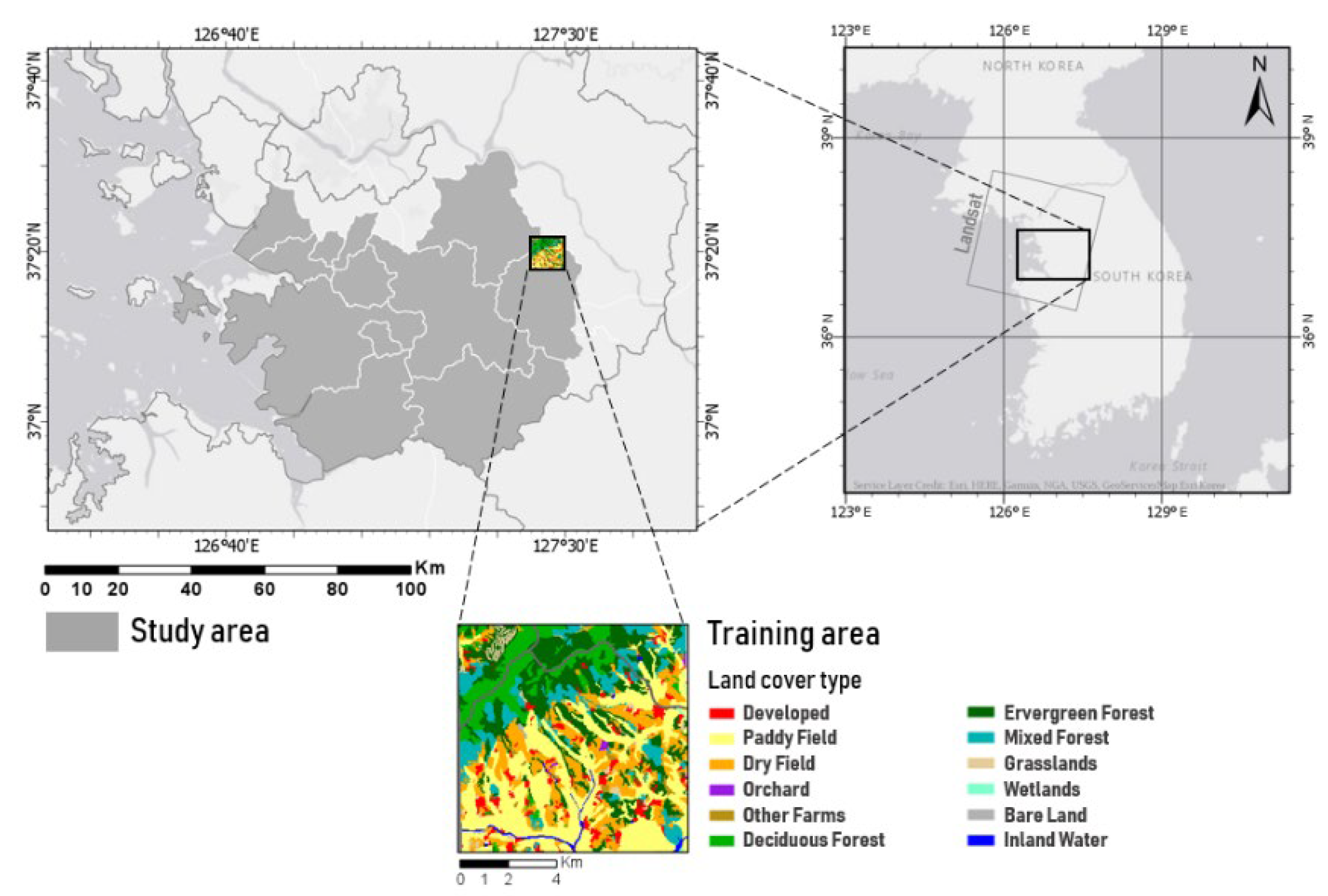
Our study area covered 12 administrative districts in the western part of Korea, where irregular droughts have occurred in spring since mid-2010. This area is located between 36°50’ N and 37°35’ N latitudes and 126°30’ E and 127°35’ E longitudes (Figure 1), has been severely affected by droughts in the springs of 2014–2017.
In the given study area, training areas for training drought should be selected based on the following criteria. First, the area with the least amount of precipitation should be selected to minimize the influence of meteorological factors. In that regard, we have reviewed all of the precipitation data [34] corresponding to the weather-observation points in the study area. Second, it needed to find a place that includes the various type of land cover. The extent should include enough sample to train the drought.
In this study, we only used a part of the study area as the training sample because we cannot control for the influence of meteorological effects for analysis; moreover, the representative of the drought function cannot be guaranteed. In addition, the use of the entire study area increases the number of training samples, which significantly increases the learning time, rendering it inefficient.
From among the candidate areas for training drought, we extracted as a square region of 7.5 km × 7.5 km (56 km2, Figure 1) as the final training area. The study area (approximately 3575 km2) is 20 times larger than the training area.
2.2. Data and Trained Drought Period
We used Landsat-8 (Level 1) and the Shuttle Radar Topography Mission (SRTM) 30 m DEM (ARC 1) data downloaded from the United States Geological Survey (USGS) EarthExplorer [35]. In addition, the land cover data for selecting the training area were retrieved from the Korea’s Environmental Information Service [36]. The software for the analysis was ArcGIS Pro version. The programming language was Python 3.6.1 version for a 64-bit Windows 10 platform.
The duration of the drought to be used for training in our study was a spring drought of approximately 3 months (97 days) corresponding to the period from 19 March 2017–23 June 2017. This period was determined by considering the date of the Landsat-8 image, drought beginning, and just before drought ending due to rain. The spring in 2017 was the worst drought since 2010, when precipitation was less than 25% of the normal annual precipitation in the study area.
2.3. Variables
We defined four categories of surface factors (i.e., vegetation, topographic, water, and thermal factor of the group) that can affect the soil moisture during short-term drought periods based on previous studies. We then selected 15 input variables corresponding to the operational definitions of the four categories mentioned earlier. Table 1 presents these variables with their abbreviations.
We calculated all the input variables as follows, according to the USGS guidelines [39] and references, as shown in Table 1. The thermal factor consists of the five bands of Landsat-8, without the calculation.
where a (m2) is the upstream contributing area and b is the slope.
where Green is a green wavelength band, which is band 3 in the Landsat-8 images.
Soil moisture can be estimated using various methods and indices, such as Soil Moisture Anomaly (SMA), Evapotranspiration Deficit Index (ETDI), Soil Moisture Deficit Index (SMDI), and Soil Water Storage (SWS) [38]. Accordingly, the appropriate indices must be selected depending on the purpose of the drought analysis [51]. We reviewed several methods to obtain the SMI for this study and found that the SMI derived by Sandholt et al. [52], calculated using NDVI and LST, using moderate-resolution satellite images, (such as Landsat-8) was the most appropriate for short-term drought prediction between spring and autumn. Welikhe et al. [49] suggested that this SMI calculation is particularly advantageous in estimating soil moisture during growing periods. The results of their study indicated that this SMI showed the highest correlation with real soil moisture at a depth of 20 cm. The formula used to calculate the SMI is presented as follows [52,53]:
where is the maximum surface temperature observation for a given NDVI, is the minimum surface temperature observation for a given NDVI.
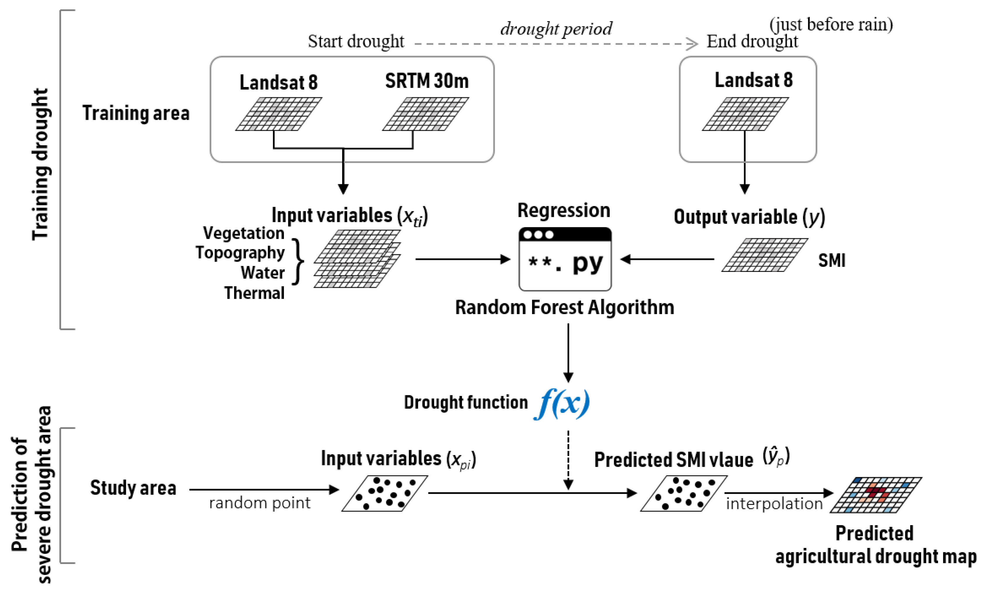
Subsequently, we constructed a drought function using the aforementioned 15 input variables of the training area on 19 March 2017 and the SMI output variables on 23 June 2017 via RF. Figure 2 shows the structure of the SDAP model including generation of the drought function and prediction of the drought-severe area.
2.4. Drought Function
We performed machine learning via RF, using 62,500 (250 × 250) data samples from the training area, in order to generate the drought function f(x). All samples were split by training (75%, n = 46,875) and test (25%, n = 15,625) datasets after 100 shuffles for all samples. We then used the RandomForestRegressor python function of the ensemble module of the scikit-learn library for machine learning. When fitting the f(x), max_depth is the most important parameter that can be used to prevent overfitting or underfitting of data during training. The optimal max_depth was 14 and was found by tuning the coefficient of determination (R2) of the training dataset maximized, while minimizing the R2 difference between the training and the test dataset.
We verified the performance of f(x) using root mean square error (RMSE), normalized RMSE (NRMSE), mean absolute error (MAE) and R2. In addition, we confirmed the spatial distribution of error by mapping.
where y is the actual SMI, ŷ is the predicted SMI, ymax is a maximum actual SMI and ymin is a minimum actual SMI.
2.5. Feature Importance
The tree-based RF regression can confirm the importance of features using the feature_importances_ function of the ensemble module of scikit-learn libraries after fitting. We found the effect of each input variable on the retention and loss of soil moisture, during non-rainfall periods, by sorting the input variables according to their individual importance using two functions. In addition, the feature’s importance of each category (i.e., vegetation, topography, water, and thermal factor) was summed to obtain the category importance order.
2.6. SMI Prediction on the Study Area
We estimated the SMI of the study area for June 2015, using the data of 14 March 2015, by applying the drought function to predict the agricultural drought of 18 June 2015. These are suitable data for predicting agricultural drought because a real drought happened in that area between March and July in 2015. The best verification for the SDAP model is the drought case since 2017, which is the year of the data source of the drought function. However, drought did not occur after 2017; hence, the closest case of the past was an alternative. As previously mentioned, prediction in this study means the future some months after; thus, the context of year does not matter.
We tried to use the Landsat-8 image on 18 June 2015 (after 97 days from 14 March 2015) for verification, but we alternatively used an image from 4 July 2015 (after 113 days from 14 March 2015) because of the many clouds in the image. For reference, the drought function trained the drought of 97 days.
The final prediction SMI map (the agricultural drought map) of the study area was obtained by the following process (see prediction section in Figure 2). We generated 400,000 random points of the study area. The predicted SMI value of those random points (ŷp) were obtained via f(x) using the input variables (xpi) on 14 March 2015. After that, the final SMI map was completed by interpolating the SMI value of the random points. We validated this predicted SMI value of random points with the actual SMI calculated using the Landsat-8 (4 July 2015) and SRTM DEM.
3. Results
3.1. Training Performance
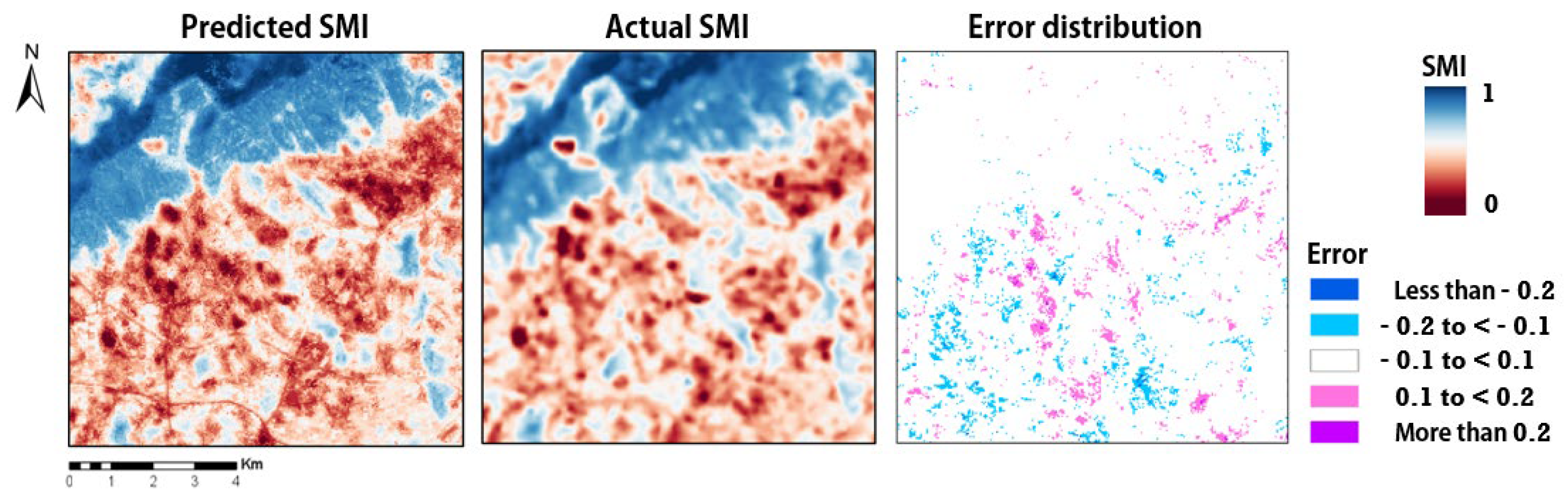
Confirmation of the training performance and error distribution of the drought function are shown in Figure 3 and Table 2. R2 showed a training performance of 0.91, and the error distribution was not concentrated on a specific land cover. Thus, it was considered to be a drought function (training area) that can represent drought in this area.
3.2. Feature Importance
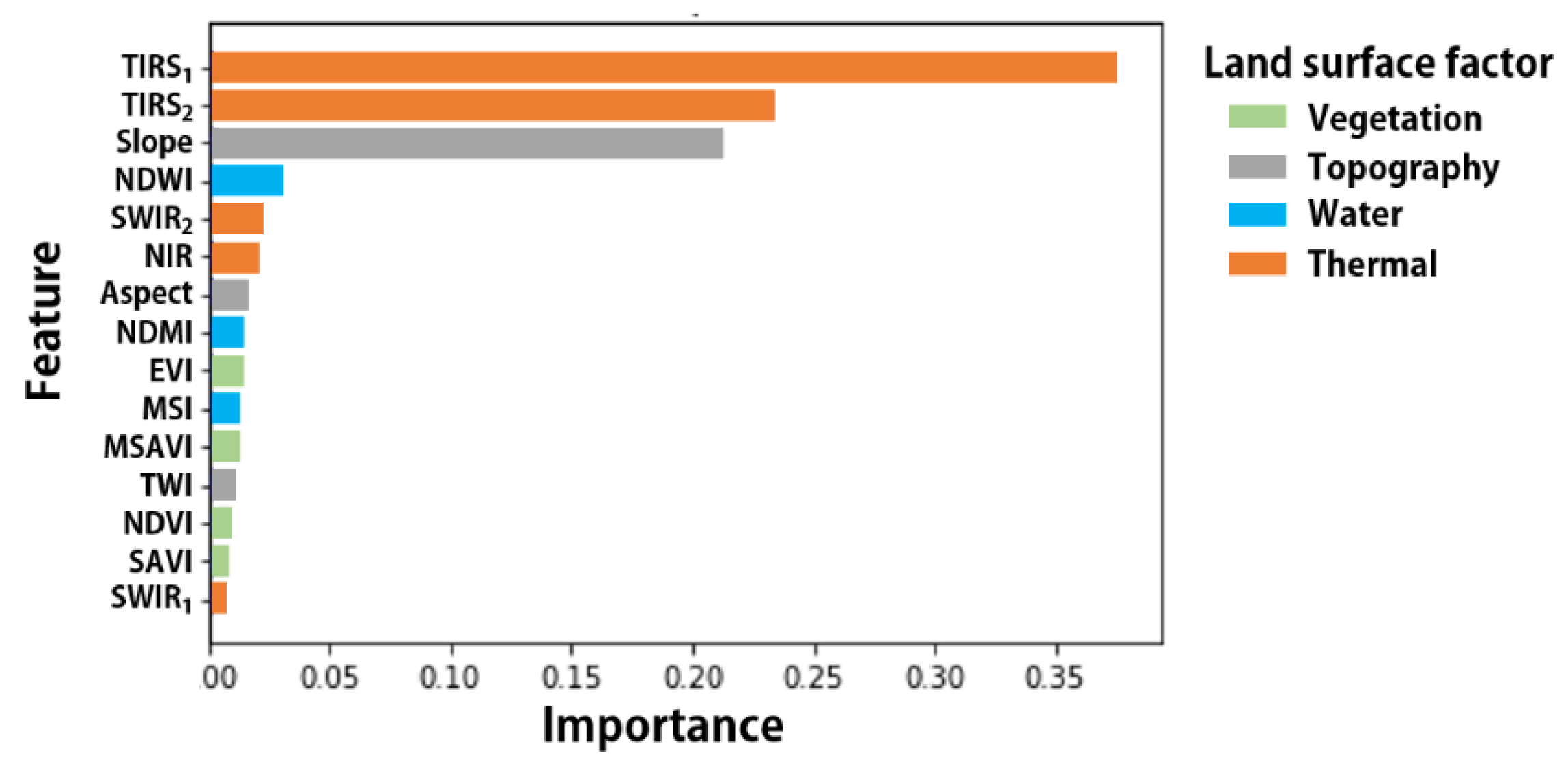
Figure 4 shows the importance of each input variable for f(x). Table 3 lists the total importance by category (i.e., thermal, water, topography, and vegetation features). The results showed that the thermal factor was the most important, but only SWIR1 had low explanatory power on the soil moisture. Particularly, among the thermal images of Landsat-8, TIRS1 was identified as a better predictor of soil moisture than TIRS2. The slope was the most important of the topographic features. The importance of water or vegetation features was similar.
3.3. SMI Prediction and Validation
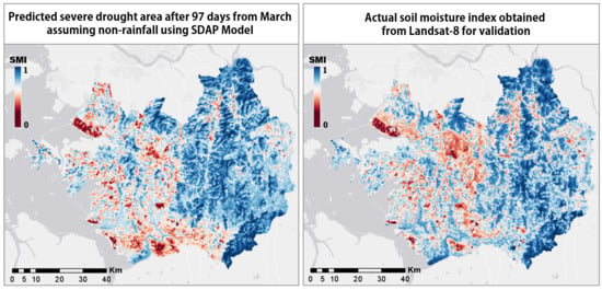
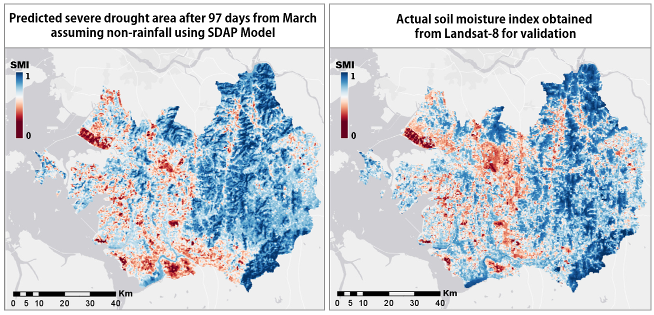
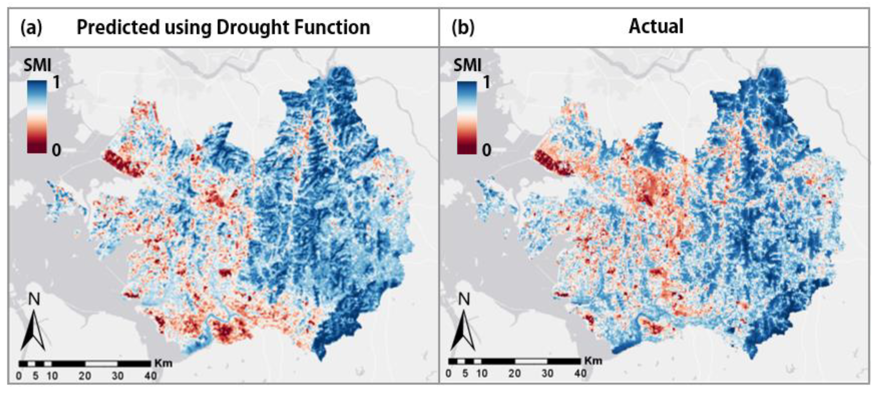
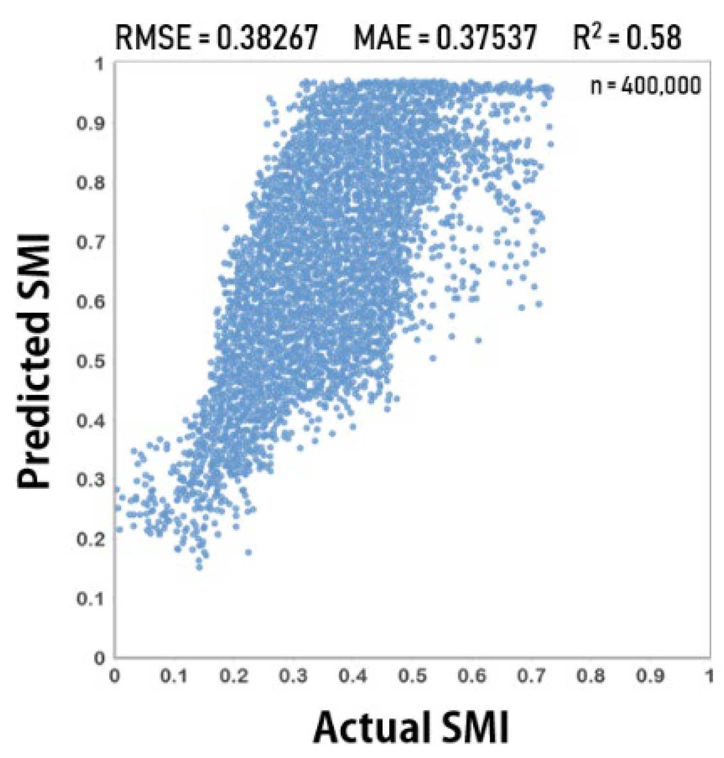
Figure 5a illustrates the map of agricultural droughts after 3 months (97 days) of non-rainfall period, predicted using the input variables of 14 March 2015 and the drought function. Figure 6 shows a scatter plot of the predicted SMI and the actual SMI for validation. From the validation results, R2 = 0.58, which was lower than the training performance (R2 = 0.91). However, it shows clearly the potential severe drought area comparing with Figure 5b as the actual SMI of drought.
4. Discussion
4.1. General Information on the SDAP Model
The appropriate training area, the selection of appropriate drought period, and the number of suitable random points to cover the study area are important in utilizing the SDAP model. Therefore, the following factors should be considered in this model. First, in the training area selection, similar proportions of different land cover types should be chosen. If a particular land cover type is dominant in the training area, the model is prone to errors in areas under the less representative land cover types. In addition, irrigated areas should be avoided to insulate against human influence on the output variable SMI.
Second, the SDAP model uses only land surface factors; hence, it is recommended to develop the drought function using data from the year in which the precipitation was the lowest (i.e., the drought year for modeling should have had the least rainfall possible for minimizing the interferences of meteorological factors). In this study, the short-term drought function was trained using data from March to June (97 days). However, drought periods can be freely selected within a one-year period (e.g., May–July), depending on the application, region, and country. It means this model has transferability to other locations with different conditions by generating drought function using the local data of the study area to be analyzed.
Third, enough random points should be allocated for the estimation and subsequent generation of the prediction map after interpolation. Given that the SMI is a float number between 0 and 1, if few points are available for estimation, the SMI pattern will not appear after the interpolation. In fact, providing a threshold for the number of appropriate points is difficult (it will vary depending on the scope of the study area and the variety of land cover). However, increasing the number of points by an adequate margin is recommended when the results do not exhibit a clear pattern. In this study, we confirmed suitable pattern generation for more than 400,000 points, whereas 300,000 points were insufficient to show the trend of agricultural drought.
4.2. Coverage of the Trained Drought Function
This study shows that the function trained by the RF algorithm was predicted as R2 = 0.58 over an area approximately 20 times larger than the training area. However, determining the predictable coverage using the trained function is difficult, given regional deviations, but prediction accuracy is negatively correlated with the distance from the training area and decreases as the prediction area increases.
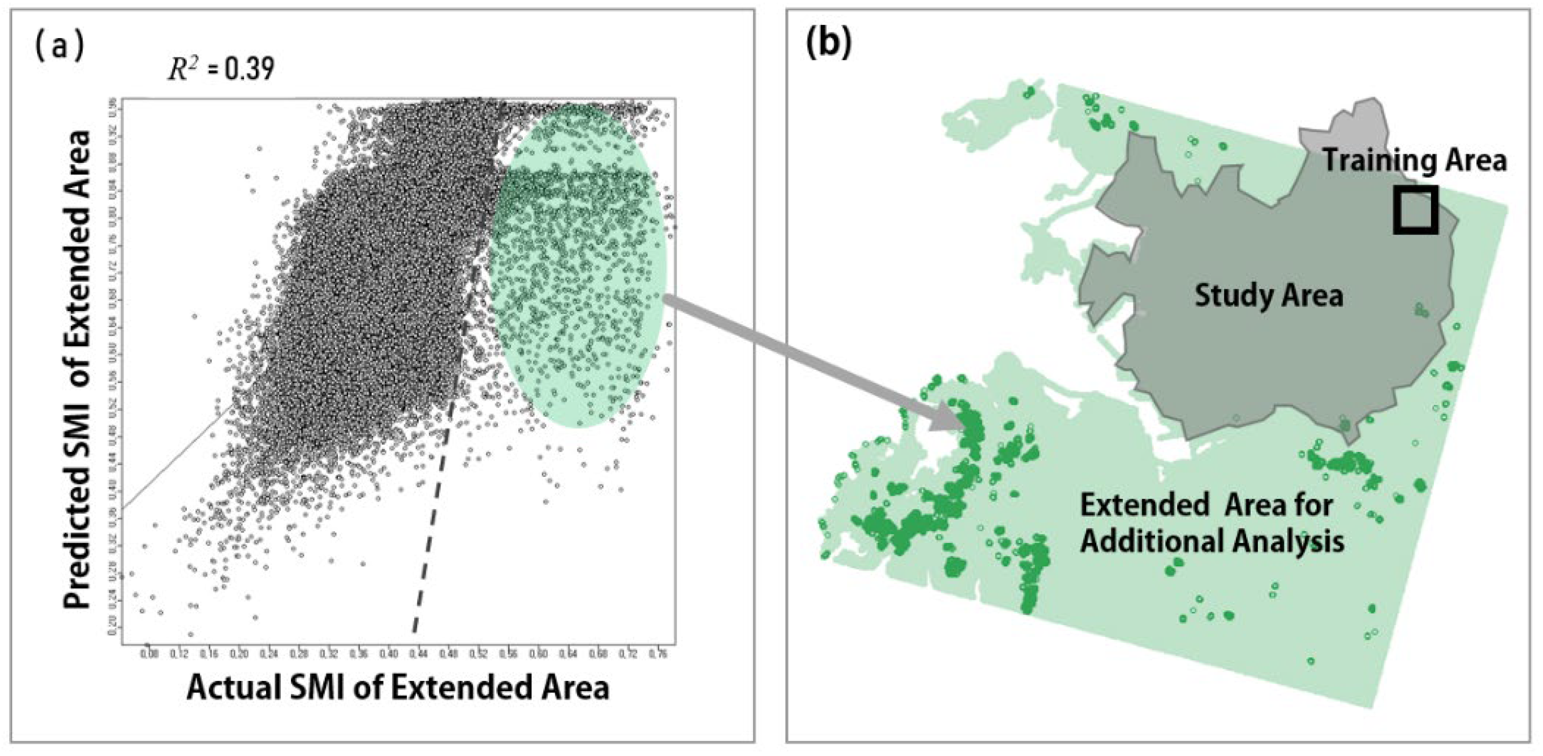
We conducted further analysis to verify the predictable coverage. We specifically predicted the SMI of a training area approximately 150 times larger than the training area and obtained a decrease in R2 from 0.58 to 0.39. As shown in Figure 7a, a region with a sharp decrease in correlation between the actual and predicted SMI was observed. The distribution of these samples was confirmed on the map. Figure 7b shows that the highest error mostly occurred far from the training area in largely heterogeneous areas. In contrast, the samples with a low correlation occurring near the training area were mostly identified as water bodies, and the error can be caused by the lack of sufficient water samples for training.
4.3. SDAP Model Advantages
4.3.1. Prediction of Severe Drought Areas
Information on drought severity is the most practical and important information for mitigating an upcoming drought [54]. The objective of this study was to predict the distribution of soil moisture assuming non-rainfall conditions. According to the National Drought Mitigation Center (NDMC), it is necessary to make a plan for drought before beginning, confirm the priority of water dependence on agriculture and the community, and to immediately apply this step-by-step when water begins to become insufficient [55]. In this step, the SDAP model can help by supporting spatial information on droughts in advance, and allow effective and planned resource allocation to reduce the impact of upcoming droughts.
The SDAP model can show future severe agricultural drought areas through non-rainfall periods because the method can reduce the uncertainty by separating two models (i.e., meteorological and agricultural droughts) with different features in the analytical results [14]. Under non-rainfall conditions, the SDAP model works on the assumption that meteorological drought forecasting is preceded. Thus, the SDAP model can analyze drought without considering meteorological data.
However, the absence of meteorological data for analysis does not mean that we have excluded climate factors. Machine learning on the growth of soil drought is a learning of the trend caused by climate and seasonal changes in the area. Therefore, the further away from the training area, the more the climate and the weather become different; hence, the prediction error of the SMI increases.
We found that one of the studies [5] predicted soil moisture using hybrid machine learning without climate data, with a similar concept to the SDAP model. However, that study cannot show the spatial distribution of the SMI because of the usage of the actual measured data from the soil of only seven points, not the remote sensing data. In fact, the prediction by [5] aimed to only predict the soil moisture of seven trained points using training data (corresponding to the validation of the performance of the drought function in our study); hence, this is just an assessment of the training performance, and not prediction. However, in our study, the training data were only used to generate the drought function, and different data from another year were used for prediction. Another study [15], using only meteorological data, cannot be used in practical drought mitigation plans because of the exclusion of the spatial distribution of agricultural drought in the prediction results.
In contrast, the results of the SDAP model can show clear SMI trends including the severe area of the SMI (Figure 5). The mitigation of Short-term drought requires the SMI spatial trend information rather than accurate SMI values [1,56]. In this model, although the SMI error (RMSE = 0.382, MAE = 0.375) of the predicted study area increased compared to the training performance of the drought function (RMSE = 0.052, MAE = 0.039), our model has achieved the aim sufficiently because it can show the agricultural drought trend clearly.
4.3.2. Feature Importance
We found that the thermal factor is one of the major factors affecting soil moisture during a drought period by confirming the findings of Sruthi and Aslam [20], who noted that increased temperature reduces soil moisture. Furthermore, TIRS1 in the thermal factor was the most important feature in the drought function (Table 3). However, one should be cautious when considering the feature importance. For example, relative vegetation features have been shown to be of low importance in our model. However, according to Sruthi and Aslam, vegetation and temperature were strongly correlated with each other [20]; hence, vegetation might play an important role in preserving soil moisture. Therefore, feature importance should be carefully considered based on other studies.
We obtained this variable importance information because we used the RF algorithm for drought training. The RF algorithm has the advantage of providing variable importance; hence, it is also used to extract important variables and remove unnecessary variables when creating a model [57]. One case involved the estimation of the relative importance of variables related to soil hydrological properties in the field of hydrology using this importance function [58].
However, whether the correlation between the SMI and feature importance is negative or positive, is unknown. Therefore, it is also helpful to reference the multi-linear regression coefficients to understand feature importance. Comparing the feature importance of the drought functions, calculated from various regions and periods, can provide important insights into drought studies related to soil moisture.
4.4. Limitations and Applications of the SDAP Model
The predicted SMI, using machine learning applied to satellite images with the resolution of 30 m, is a suitable drought information for planning the mitigation of short-term drought at the regional level because the local spatial distribution is acquired. However, some general remote sensing limitations exist, such as difficulty in obtaining data of the right date to be analyzed because of cloud or revisit cycle of the Landsat-8. This limitation can be addressed by considering using other satellite images with a higher temporal resolution. This solution remains to be confirmed in further studies. Along with the general limitations of remote sensing, this SDAP model has the following limitations:
First, the SDAP model applies only to the prediction of short-term droughts, within several months, because the SMI is a suitable measure for that timescale [49]. In practice, the soil will become dry, regardless of the surface state if non-rainfall conditions persist for longer periods. Therefore, the SDAP model is suitable for short-term droughts that can be mitigated by human action within a few months.
Second, the prediction of droughts may be difficult if the area has no drought experience or different seasons, because this model is based on learning from past droughts. Therefore, various drought functions by period or season must be considered to make a suitable prediction of the situation.
Third, this model must be based on a sequential approach to finding solutions by analyzing droughts by each expert group. Thus, it is not suitable for an integrated method of calculating meteorological, agricultural, and hydrological droughts at one time because this model predicts the trend of agricultural drought change after the meteorological drought analysis is preceded. For example, the spatial information of agricultural drought, which is the result of this model, is then subject to a primary review against the corresponding hydrological drought. After all the analyses have been conducted, and the areas of concern droughts have been identified, priority plans for water reserves (e.g., water demand control) and water allocation for these areas should be established. Therefore, the proposed model is only suitable to prepare for short-term droughts and find focalized solutions by each expert group, instead of performing an integrated analysis of various models with high uncertainty.
5. Conclusions
Agricultural drought is a disaster that must be managed effectively as it directly affects food security. For this reason, several models have been developed to predict agricultural drought. However, regardless of how good a model is, inaccuracies arise in the prediction of droughts, due to meteorological anomalies where the model is based on repeated patterns or historical precipitation data. The proposed SDAP model was hence developed by accepting those uncertainties, rather than overcome meteorological uncertainties. This SDAP model does not depend on precipitation data because it predicts potential drought-severe areas under the assumption that rainfall-deficit conditions already exist.
In addition, existing other models can be catastrophic in the event that an unpredicted drought occurs. However, given that it makes prediction under the condition of no rainfall such as that done in our model, there is a benefit for society even if no drought occurs. Although our model is designed for a short-term drought, accumulation of these predictions also helps us identify areas that are susceptible to drought so that mitigation plans can be prepared from a long-term perspective.
Given that the ultimate objective for predicting droughts is to develop mitigation plans, the model must be a simple, practical, and useful such as the SDAP model. This model is easy to understand as it uses a regression algorithm compared to other huge prediction systems. Further, the analysis of various case studies for many regions and drought functions in SDAP model can provide meaningful insights into the key factors associated with drought. At present, we are working on a comparison study of machine learning algorithms to improve the SDAP model as well as a case study involving the application of the SDAP model.
Author Contributions
Model design, data collection, Python coding, data analysis, validation, mapping, and writing, H.P.; manuscript review and advice on statistics, K.K.; supervision, D.k.L.
Funding
This subject is supported by Korea Ministry of Environment (MOE, Project No. 2016000210004) as “Public Technology Program based on Environmental Policy”.
Acknowledgments
This research was awarded by the Korea Ministry of the Interior and Safety in the “Disaster Safety Research Paper Contest” in 2018. This manuscript was written by developing a part of the research as a prediction model. This SDAP model is patent pending. You can freely reference this manuscript and model, but if you copy our idea as your own, without citation, legal action may be taken.
Conflicts of Interest
The authors declare no conflict of interest.
References
- Hao, Z.; Singh, V.P.; Xia, Y. Seasonal Drought Prediction: Advances, Challenges, and Future Prospects. Rev. Geophys. 2018, 56, 108–141. [Google Scholar] [CrossRef]
- Mishra, A.K.; Desai, V.R. Drought forecasting using stochastic models. Stoch. Environ. Res. Risk Assess. 2005, 19, 326–339. [Google Scholar] [CrossRef]
- Schepen, A.; Wang, Q.J.; Robertson, D.E. Combining the strengths of statistical and dynamical modeling approaches for forecasting Australian seasonal rainfall. J. Geophys. Res. Atmos. 2012, 117, 1–9. [Google Scholar] [CrossRef]
- Hao, Z.; Xia, Y.; Luo, L.; Singh, V.P.; Ouyang, W.; Hao, F. Toward a categorical drought prediction system based on U.S. Drought Monitor (USDM) and climate forecast. J. Hydrol. 2017, 551, 300–305. [Google Scholar] [CrossRef]
- Prasad, R.; Deo, R.C.; Li, Y.; Maraseni, T. Soil moisture forecasting by a hybrid machine learning technique: ELM integrated with ensemble empirical mode decomposition. Geoderma 2018, 330, 136–161. [Google Scholar] [CrossRef]
- Rezaeianzadeh, M.; Stein, A.; Cox, J.P. Drought Forecasting using Markov Chain Model and Artificial Neural Networks. Water Resour. Manag. 2016, 30, 2245–2259. [Google Scholar] [CrossRef]
- Predicting Droght. Available online: http://drought.unl.edu/DroughtBasics/PredictingDrought.aspx (accessed on 19 January 2018).
- Cook, B.I.; Smerdon, J.E.; Seager, R.; Coats, S. Global warming and 21st century drying. Clim. Dyn. 2014, 43, 2607–2627. [Google Scholar] [CrossRef]
- Wilhite, D.; Glantz, M. Understanding: The Drought Phenomenon: The Role of Definitions. Water Int. 1985, 10, 111–120. [Google Scholar] [CrossRef]
- Park, S.; Im, J.; Jang, E.; Rhee, J. Drought Assessment and Monitoring through Blending of Multi-sensor Indices Using Machine Learning Approaches for Different Climate Regions. Agric. For. Meteorol. 2016, 217, 50. [Google Scholar] [CrossRef]
- Mishra, A.K.; Desai, V.R.; Singh, V.P. Drought Forecasting Using a Hybrid Stochastic and Neural Network Model. J. Hydrol. Eng. 2007, 12, 626–638. [Google Scholar] [CrossRef]
- Durdu, Ö.F. Application of linear stochastic models for drought forecasting in the Büyük Menderes river basin, western Turkey. Stoch. Environ. Res. Risk Assess. 2010, 24, 1145–1162. [Google Scholar] [CrossRef]
- Ali, Z.; Hussain, I.; Faisal, M.; Nazir, H.M.; Hussain, T.; Shad, M.Y.; Mohamd Shoukry, A.; Hussain Gani, S. Forecasting Drought Using Multilayer Perceptron Artificial Neural Network Model. Adv. Meteorol. 2017, 2017. [Google Scholar] [CrossRef]
- Mastrandrea, M.D.; Mach, K.J.; Plattner, G.; Matschoss, P.R. The IPCC AR5 guidance note on consistent treatment of uncertainties: A common approach across the working groups. Clim. Chang. 2011, 108, 675–691. [Google Scholar] [CrossRef]
- Maity, R.; Suman, M.; Verma, N.K. Drought prediction using a wavelet based approach to model the temporal consequences of different types of droughts. J. Hydrol. 2016, 539, 417–428. [Google Scholar] [CrossRef]
- Fung, K.F.; Huang, Y.F.; Koo, C.H.; Soh, Y.W. Drought forecasting: A review of modelling approaches 2007–2017. J. Water Clim. Chang. 2019. [Google Scholar] [CrossRef]
- Olang, L.; Ali, A.; Demuth, S.; Wood, E.F.; Yuan, X.; Sadri, S.; Chaney, N.; Guan, K.; Sheffield, J.; Amani, A.; et al. A Drought Monitoring and Forecasting System for Sub-Sahara African Water Resources and Food Security. Bull. Am. Meteorol. Soc. 2013, 95, 861–882. [Google Scholar] [CrossRef]
- Hao, Z.; AghaKouchak, A.; Nakhjiri, N.; Farahmand, A. Global integrated drought monitoring and prediction system. Sci. Data 2014, 1, 140001. [Google Scholar] [CrossRef]
- Causes of Drought: What’s the Climate Connection. Available online: http://www.ucsusa.org/global_warming/science_and_impacts/impacts/causes-of-drought-climate-change-connection.html#.VPXWTFPF_40%5Cnhttp://www.ucsusa.org/global_warming/science_and_impacts/impacts/causes-of-drought-climate-change-connection.html%23.VpAtT1JK7w (accessed on 19 January 2018).
- Sruthi, S.; Aslam, M.A.M. Agricultural Drought Analysis Using the NDVI and Land Surface Temperature Data; a Case Study of Raichur District. Aquat. Procedia 2015, 4, 1258–1264. [Google Scholar] [CrossRef]
- Raduła, M.W.; Szymura, T.H.; Szymura, M. Topographic wetness index explains soil moisture better than bioindication with Ellenberg’s indicator values. Ecol. Indic. 2018, 85, 172–179. [Google Scholar] [CrossRef]
- Park, H.; Lee, D. Disaster Prediction and Policy Simulation for Evaluating Mitigation Effects Using Machine Learning and System Dynamics: Case Study of Seasonal Drought in Gyeonggi Province. J. Korean Soc. Hazard Mitig 2019, 19, 45–53. [Google Scholar] [CrossRef]
- Breiman, L. Random forests. Mach. Learn. 2001, 45, 5–32. [Google Scholar] [CrossRef]
- Rhee, J.; Im, J. Meteorological drought forecasting for ungauged areas based on machine learning: Using long-range climate forecast and remote sensing data. Agric. For. Meteorol. 2017, 237–238, 105–122. [Google Scholar] [CrossRef]
- Danandeh Mehr, A.; Kahya, E.; O¨zger, M. A gene-wavelet model for long lead time drought forecasting. J. Hydrol. 2014, 517, 691–699. [Google Scholar] [CrossRef]
- DeChant, C.M.; Moradkhani, H. Analyzing the sensitivity of drought recovery forecasts to land surface initial conditions. J. Hydrol. 2015, 526, 89–100. [Google Scholar] [CrossRef]
- Zhu, Y.; Wang, W.; Singh, V.P.; Liu, Y. Combined use of meteorological drought indices at multi-time scales for improving hydrological drought detection. Sci. Total Environ. 2016, 571, 1058–1068. [Google Scholar] [CrossRef]
- Yu, C.; Li, C.; Xin, Q.; Chen, H.; Zhang, J.; Zhang, F.; Li, X.; Clinton, N.; Huang, X.; Yue, Y.; et al. Dynamic assessment of the impact of drought on agricultural yield and scale-dependent return periods over large geographic regions. Environ. Model. Softw. 2014, 62, 454–464. [Google Scholar] [CrossRef]
- Park, S.; Seo, E.; Kang, D.; Im, J. Prediction of Drought on Pentad Scale Using Remote Sensing Data and MJO Index through Random Forest over East Asia. Remote Sens. 2018, 10, 1811. [Google Scholar] [CrossRef]
- AghaKouchak, A. A baseline probabilistic drought forecasting framework using standardized soil moisture index: Application to the 2012 United States drought. Hydrol. Earth Syst. Sci. 2014, 18, 2485–2492. [Google Scholar] [CrossRef]
- Hao, Z.; Hao, F.; Singh, V.P.; Ouyang, W.; Cheng, H. An integrated package for drought monitoring, prediction and analysis to aid drought modeling and assessment. Environ. Model. Softw. 2017, 91, 199–209. [Google Scholar] [CrossRef]
- Mo, K.C.; Shukla, S.; Lettenmaier, D.P.; Chen, L.C. Do Climate Forecast System (CFSv2) forecasts improve seasonal soil moisture prediction? Geophys. Res. Lett. 2012, 39, 1–6. [Google Scholar] [CrossRef]
- Schäfer, D.; Samaniego, L.; Kumar, R.; Mai, J.; Thober, S.; Sheffield, J. Seasonal Soil Moisture Drought Prediction over Europe Using the North American Multi-Model Ensemble (NMME). J. Hydrometeorol. 2015, 16, 2329–2344. [Google Scholar] [CrossRef]
- Korean Statistical Information Service (KOSIS). Available online: http://kosis.kr (accessed on 14 May 2018).
- Earth Explorer. Available online: https://earthexplorer.usgs.gov (accessed on 11 May 2018).
- Environmental Geographic Information Service (EGSI). Available online: https://egis.me.go.kr (accessed on 2 May 2018).
- Huete, A.; Didan, K.; Miura, T.; Rodriguez, E.P.; Gao, X.; Ferreira, L.G. Overview of the radiometric and biophysical performance of the MODIS vegetation indices. Remote Sens. Environ. 2002, 83, 195–213. [Google Scholar] [CrossRef]
- Handbook of Drought Indicators and Indices; World Meteorologcal Organizatio (WMO): Geneva, Switzerland; Global Water Partnership (GWP): Stockholm, Sweden, 2016; ISBN 978-92-63-11173-9.
- Product Guide: Landsat Surface Reflectance-Derived Spectral Indices; 3.6 Version; Department of the Interior U.S. Geological Survey (USGS): Reston, VA, USA, 2017.
- Tucker, C.J. Red and photographic infrared linear combinations for monitoring vegetation. Remote Sens. Environ. 1979, 8, 127–150. [Google Scholar] [CrossRef]
- Sydney, T. A Soil-Adjusted Vegetation Index (SAVI). Remote Sens. Environ. 1988, 25, 295–309. [Google Scholar] [CrossRef]
- Qi, J.; Chehbouni, A.; Huete, A.R.; Kerr, Y.H.; Sorooshian, S. A modified soil adjusted vegetation index. Remote Sens. Environ. 1994, 48, 119–126. [Google Scholar] [CrossRef]
- Beven, K.J.; Kirkby, M.J. A physically based, variable contributing area model of basin hydrology. Hydrol. Sci. Bull. 1979, 24, 43–69. [Google Scholar] [CrossRef]
- Burrough, P.A.; Mcdonnell, R.A. Data Models and Axioms. Princ. Geogr. Inf. Syst. 1998, 17–34. [Google Scholar] [CrossRef]
- How Slope Works. Available online: http://desktop.arcgis.com/en/arcmap/10.3/tools/spatial-analyst-toolbox/how-slope-works.htm (accessed on 21 December 2018).
- How Aspect Works. Available online: http://pro.arcgis.com/en/pro-app/tool-reference/spatial-analyst/how-aspect-works.htm (accessed on 21 December 2018).
- Gao, B. NDWI—A normalized difference water index for remote sensing of vegetation liquid water from space. Remote Sens. Environ. 1996, 58, 257–266. [Google Scholar] [CrossRef]
- Xu, H. Modification of normalised difference water index (NDWI) to enhance open water features in remotely sensed imagery. Int. J. Remote Sens. 2006, 27, 3025–3033. [Google Scholar] [CrossRef]
- Welikhe, P.; Quansah, J.E.; Fall, S.; McElhenney, W. Estimation of Soil Moisture Percentage Using LANDSAT-based Moisture Stress Index. J. Remote Sens. GIS 2017, 06. [Google Scholar] [CrossRef]
- Bands Specifications of Landsat 8. Available online: https://landsat.usgs.gov/provisional-landsat-8-surface-reflectance-data-available (accessed on 19 December 2018).
- Mishra, A.K.; Singh, V.P. A review of drought concepts. J. Hydrol. 2010, 391, 202–216. [Google Scholar] [CrossRef]
- Sandholt, I.; Rasmussen, K.; Andersen, J. A simple interpretation of the surface temperature/vegetation index space for assessment of surface moisture status. Remote Sens. Environ. 2002, 79, 213–224. [Google Scholar] [CrossRef]
- Zeng, Y.N.; Feng, Z.D.; Xiang, N.P. Assessment of soil moisture using Landsat ETM+ temperature/vegetation index in semiarid environment. IEEE Int. Geosci. Remote Sens. Symp. Proc. 2004, 1–7, 4306–4309. [Google Scholar] [CrossRef]
- Panu, U.S.; Sharma, T.C. Challenges in drought research: Some perspectives and future directions. Hydrol. Sci. J. 2002, 47, S19–S30. [Google Scholar] [CrossRef]
- National Drought Mitigation Center(NDMC), Drought Basics. Available online: https://drought.unl.edu/Education/DroughtBasics.aspx (accessed on 26 December 2018).
- Leeuwen, B. Van GIS workflow for continuous soil moisture estimation based on medium resolution satellite data. In Proceedings of the 18th AGILE International Conference on Geographic Information Science, Lisbon, Portugal, 9–12 June 2015. [Google Scholar]
- Gregorutti, B.; Michel, B.; Saint-Pierre, P. Correlation and variable importance in random forests. Stat. Comput. 2017, 27, 659–678. [Google Scholar] [CrossRef]
- Thompson, J.A.; Roecker, S.; Grunwald, S.; Owens, P.R. Chapter 21—Digital Soil Mapping: Interactions with and Applications for Hydropedology; Academic Press: Boston, MA, USA, 2012; pp. 665–709. ISBN 978-0-12-386941-8. [Google Scholar]
Figure 1.
Study and training areas for short-term agricultural drought prediction.

Figure 2.
Structure of the severe drought area prediction (SDAP) model. xti: input variable of the training area; y: actual soil moisture index (SMI); xpi: input variable of the study area; and ŷp: predicted SMI of the study area.
Figure 2.
Structure of the severe drought area prediction (SDAP) model. xti: input variable of the training area; y: actual soil moisture index (SMI); xpi: input variable of the study area; and ŷp: predicted SMI of the study area.

Figure 3.
Verification of the training performance and error distribution.

Figure 4.
Feature importance of drought function.

Figure 5.
Final predicted SMI map and actual SMI. The predicted map shows the soil moisture state of the study area assuming non-rainfall during 97 days using the drought function and input variables of 14 March 2015. Actual SMI map calculated from the Landsat-8 images on 4 July 2015, 119 days after 14 March 2015.

Figure 6.
Scatter plot between the actual and the predicted SMI of the study area. As a result of the validation, R2 was 0.58 and the predicted value tended to be slightly higher than the observed.
Figure 6.
Scatter plot between the actual and the predicted SMI of the study area. As a result of the validation, R2 was 0.58 and the predicted value tended to be slightly higher than the observed.

Figure 7.
(a) Relation between the actual and predicted SMI over an area 150 times (8249 km2) larger than the training area; (b) Distance from the training area and distribution of erroneous samples.
Figure 7.
(a) Relation between the actual and predicted SMI over an area 150 times (8249 km2) larger than the training area; (b) Distance from the training area and distribution of erroneous samples.


Table 1.
Feature categories and their input variables.
| Land Surface Factors | Input Variables (15) | Abbreviation | Data |
|---|---|---|---|
| Vegetation 1 | Enhanced vegetation index [37,38,39] | EVI | Band 2, 4, 5 |
| Normalized difference vegetation Index [38,39,40] | NDVI | Band 4, 5 | |
| Soil-adjusted vegetation index [38,39,41] | SAVI | Band 4, 5 | |
| Modified soil-adjusted vegetation index [39,42] | MSAVI | Band | |
| Topography 2 | Topographic wetness index [43] | TWI | SRTM DEM |
| Slope [44,45] | SRTM DEM | ||
| Aspect [44,46] | SRTM DEM | ||
| Water 3 | Normalized difference moisture index [39,47] | NDMI | Band 5, 6 |
| Modification of normalized difference water index [48] | MNDWI | Band 3, 6 | |
| Moisture stress index [49] | MSI | Band 5, 6 | |
| Thermal 4 | Near infrared [50] | NIR | Band 5 |
| Short-wavelength infrared 1 [50] | SWIR1 | Band 6 | |
| Short-wavelength infrared 2 [50] | SWIR2 | Band 7 | |
| Thermal infrared 1 [50] | TIRS1 | Band 10 | |
| Thermal infrared 2 [50] | TIRS2 | Band 11 |
1 This factor limit soil moisture loss; 2 this factor is affecting soil moisture content; 3 this factor is related to surface water; 4 this factor is related to the soil moisture evaporation.
Table 2.
Evaluation of the training performance of the drought function.
| RMSE | NRMSE | MAE | R2 | Max. SMI 1 | Min. SMI 2 | Max. Error |
|---|---|---|---|---|---|---|
| 0.05294 | 5.29% | 0.03980 | 0.91 | 0.97940 | 0.05684 | 0.30352 |
1 The actual maximum SMI value is 1; 2 The actual minimum SMI value is 0.
Table 3.
The importance of land surface factor on drought function.
| Land Surface Factors | Importance |
|---|---|
| Thermal | 0.659 |
| Topography | 0.238 |
| Water | 0.059 |
| Vegetation | 0.044 |
© 2019 by the authors. Licensee MDPI, Basel, Switzerland. This article is an open access article distributed under the terms and conditions of the Creative Commons Attribution (CC BY) license (http://creativecommons.org/licenses/by/4.0/).
Share and Cite
MDPI and ACS Style
Park, H.; Kim, K.; Lee, D.k. Prediction of Severe Drought Area Based on Random Forest: Using Satellite Image and Topography Data. Water 2019, 11, 705. https://doi.org/10.3390/w11040705
AMA Style
Park H, Kim K, Lee Dk. Prediction of Severe Drought Area Based on Random Forest: Using Satellite Image and Topography Data. Water. 2019; 11(4):705. https://doi.org/10.3390/w11040705
Chicago/Turabian StylePark, Haekyung, Kyungmin Kim, and Dong kun Lee. 2019. "Prediction of Severe Drought Area Based on Random Forest: Using Satellite Image and Topography Data" Water 11, no. 4: 705. https://doi.org/10.3390/w11040705
Note that from the first issue of 2016, this journal uses article numbers instead of page numbers. See further details here.