Correction and Informed Regionalization of Precipitation Data in a High Mountainous Region (Upper Indus Basin) and Its Effect on SWAT-Modelled Discharge


1
Department of Geohydraulics and Engineering Hydrology, University of Kassel, 34127 Kassel, Germany
2
Department of Environmental Sciences, COMSATS University Islamabad, Abbottabad Campus, University Road, Abbottabad 22060, Pakistan
*
Author to whom correspondence should be addressed.
Water 2018, 10(11), 1557; https://doi.org/10.3390/w10111557
Submission received: 12 September 2018
/
Revised: 27 October 2018
/
Accepted: 30 October 2018
/
Published: 1 November 2018
(This article belongs to the Section Hydrology)
Abstract
:The current study applied a new approach for the interpolation and regionalization of observed precipitation series to a smaller spatial scale (0.125° by 0.125° grid) across the Upper Indus Basin (UIB), with appropriate adjustments for the orographic effect and changes in glacier storage. The approach is evaluated and validated through reverse hydrology, and is guided by observed flows and the available knowledge base. More specifically, the generated corrected precipitation data is validated by means of SWAT-modelled responses of the observed flows to the different input precipitation series (original and corrected ones). The results show that the SWAT-simulated flows using the corrected, regionalized precipitation series as input are much more in line with the observed flows than those using the uncorrected observed precipitation input for which significant underestimations are obtained.
1. Introduction
Water balance calculations and spatially distributed rainfall-runoff models require high resolution climatic datasets as a primary input. The quality of climatic forcing input is certainly the most important factor capable of influencing the simulation results [1,2,3,4,5,6,7], so that any errors in the input (climatic data) are amplified in the output (simulated hydrology) [8]. Among the climatic forcing data, precipitation and temperature are the most vital climatic variables as they directly influence the catchment discharge [9] through direct runoff, evapotranspiration losses or the snow and glacier melt contributions.
As precipitation is extremely variable in terms of spatial and temporal distribution, over mountainous catchments, it is extremely challenging to assess its true spatial distribution, especially when there is a limited spatial density of available gauging networks [10], and the then usually used “valley based” gauging networks are mostly unable to capture the orographic influences. The problem can be further exacerbated when the precipitation dataset has quality issues or temporal discontinuities. The hydrological investigations in such mountainous catchments may therefore find “water imbalances”, with higher streamflow totals, in excess of precipitation-based estimates.
The precipitation data for the Upper Indus Basin (UIB) also suffer from these problems and the sparsely located, often lower-altitude, in-situ observational network, is unable to provide precipitation time series with the appropriate spatial, altitudinal and temporal coverage. This poses one of the major hindrances for carrying out hydro-meteorological investigations and climate change impact studies in the UIB. The climate station network in the UIB has historically been comprised of very few low-altitude, valley-based stations. Although the number of in-situ observational points has increased since the mid-90s, with the installations of a few higher—altitude, automatic weather stations, the coverage is still very thin and the data less representative, especially, for different elevation zones. The available data also needs a lot of preprocessing, as it represents uncorrected raw precipitation readings, and, therefore, needs checking for quality issues and correction for losses or gaps. Similarly, while most of the weather stations have become operational after the mid-90s, long-term data is a rare commodity and is only available at a limited number of locations.
Owing to the complex orography of the UIB region and to the co-action of different hydro-climatic regimes (which affect the amounts, spatial patterns and the seasonality of precipitation), neither the sparse observed station data (or the gridded data products based on them) nor the sensors-based data, fully represents the precipitation regime of the region [11,12,13,14]. Several studies have pointed out that precipitation in the Hindu Kush Himalayan (HKH) region exhibits large changes over short distances and has a considerable vertical gradient [15,16,17,18,19,20]. This also explains the fact that the average precipitation amounts over the UIB (based on the sparse and low-altitude climatic station network) are unrealistically low to be able to sustain the observed discharge at the basin outlet.
These factors have led many researchers to find ways to assess methods for precipitation correction that may lead to a more realistic water balance [21] in many basins and have also compelled a number of hydrological studies in the UIB region to use, in addition to the observed station data, a variety of other reference climate data from different sources, either directly or with prior modifications and adjustments (e.g., TRMM Data [22]; modified APHRODIT [23], or modified WFDEI data [13] etc.).
This study proposes a simple method to regionalize and correct precipitation data in the UIB through accounting for the orographic effect at a scale finer than the one covered by the stream-gauging network, by applying a new method based on a step-wise correction and informed regionalization. This method consists of three steps: (1) Correction for systematic errors; (2) backward hydrology estimation to detect underestimation in the observed precipitation; and (3) interpolation/regionalization of the precipitation along with application of a correction factor.
Although the corrected precipitation data generated in this way may not be explicitly correct at a very fine spatial scale, it is expected to produce reasonably accurate precipitation data by accounting for the orographic effect at gauged-catchment scale and, therefore, should probably be better than that produced by other methods and, with that, be especially suitable for use in hydrological modeling and simulations. Additionally, for the time-period before the installation of the new and denser climatic network (1961–1996), precipitation data are reconstructed at the locations of the newer installations, guided by the station data collected after that period, prior to the application of regionalization and correction for the orographic effect.
While the proposed correction method is applied to precipitation data in the UIB as the present study area, it can easily be replicated in any basin with apparent altitudinal orographic effects or shortages of long term data.
2. Study Area and Data
2.1. Study Area—The Upper Indus River Basin (UIB)
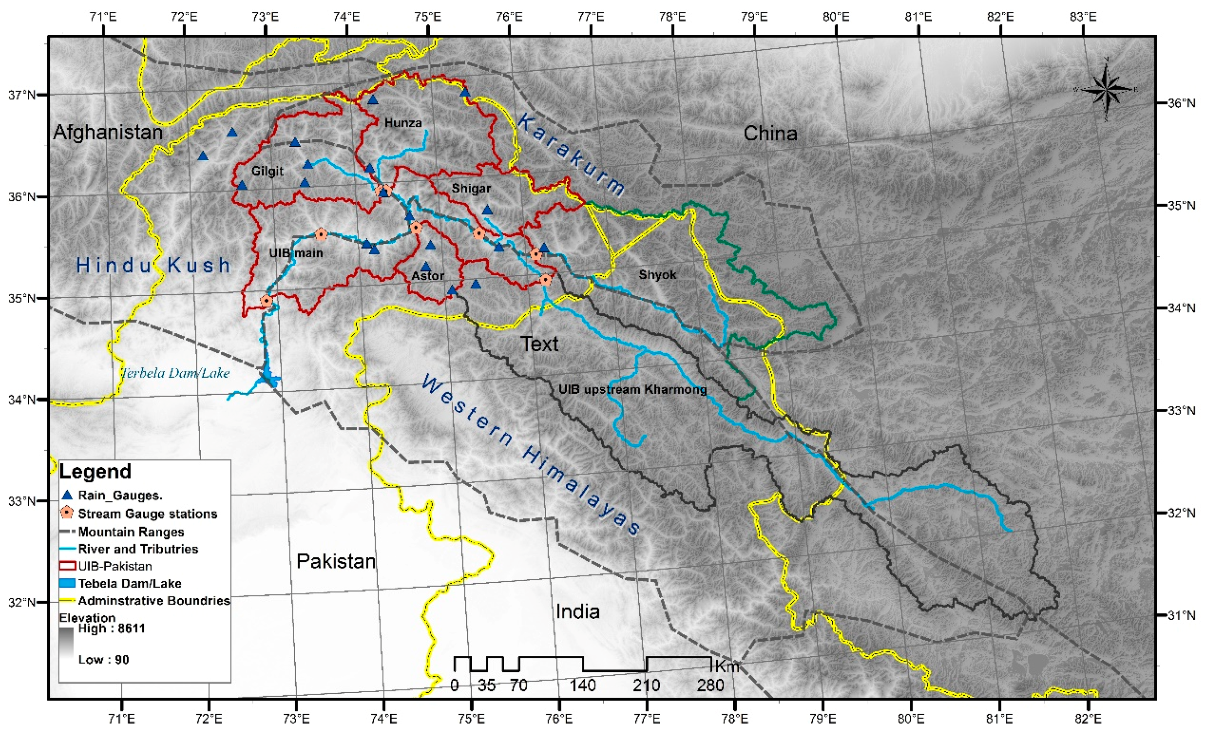
With a total length of about 2880 km and a drainage area of about 912,000 km2, the Indus River is one of the largest rivers in Asia, extending across portions of India, China, Pakistan and Afghanistan [24]. The portion of the Indus basin upstream of the Tarbela Dam (Figure 1) comprises the upper Indus river basin (UIB). The length of the river until that dam is about 1150 km, and it drains an area of about 165,400 km2 as per our findings.
Being a high-mountain region, the UIB contains the greatest area of perennial glacial ice cover (~15,062 km2) outside the polar regions, with 2174 km3 of total ice reserves [25]. Some estimates [26] show even greater glacier cover, reaching up to 12% of the UIB (above 19,000 km2). The altitude within the UIB ranges from as low as 455 m to a high of 8611 m and, as a result, the climate varies greatly within the basin [27].
The summer monsoon has little effect on the basin, as almost 90% is in the rain shadow of the Himalayan belt [22]. Except for the south-facing foothills, the intrusion of the
Indian-ocean monsoon is limited by the mountains, so that its influence weakens north-westward [28]. Subsequently, the climatic controls in the UIB are quite different from that in the Himalayas on the eastern side. In fact, over the extent of the UIB, most of the annual precipitation originates in the west, resulting from the mid-latitude western disturbances, and mostly in solid form during winter and spring [19,20,29,30]. Occasional rains are brought by the monsoonal incursions to trans-Himalayan areas [20,29], but even during the summer months, the trans-Himalayan areas do not derive all precipitation from monsoon sources [31].
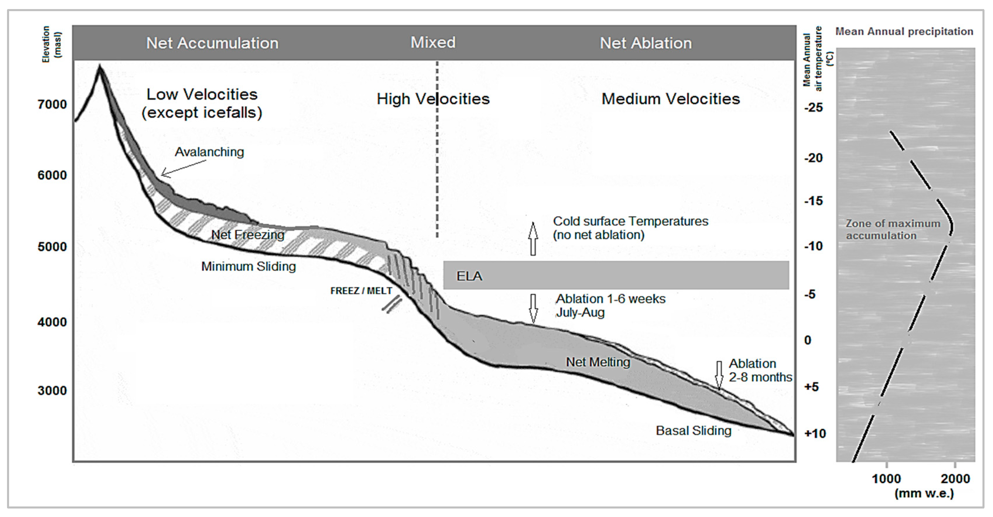
Climatic variables are usually strongly influenced by topographic altitude. Thus, the northern valley floors of the UIB are arid, with annual precipitation of only 100–200 mm. These totals increase to 600 mm at 4400 m elevation, and glaciological studies suggest annual accumulation rates of 1500 to 2000 mm at 5500 m altitude [20,32] (see Appendix A—Figure A1)
The average snow cover area in the UIB changes from 10% to 70%, with a maximum of 70‒80% in the winter snow accumulation period (December to February) and a minimum of 10‒15% in the summer snow melt period (June to September) [27]. Stream flow is generated by the combination of the storm runoff in the lower part of the upper Indus basin and the snow and glacier runoff from the higher parts of the UIB [24,33]. Nearly half of the total annual flow in the Indus basin as a whole is contributed to by the UIB, with a 86–88% contribution during the summer season while only a 12–14% contribution during the winter season [34,35].
2.2. Observed Hydro-Climatic Data
2.2.1. Observed Precipitation Data
The precipitation data of 20 meteorological stations (Figure 1), operative in the study area (UIB), were used in this study. Out of these stations, six are operated by the Pakistan Meteorological Organization (PMD), while 14 relatively new stations are under the jurisdiction of the Water & Power Development Authority, Pakistan (WAPDA).
The stations operated by PMD have long term precipitation records (1947 to date), but were not corrected for under-catch and occasional gaps and temporal discontinuities in the records. The recent PMD-station records, although fairly consistent, are all from low altitude stations, unable to represent precipitation regimes of higher altitudes. The other 14 climate stations are fairly new and are installed specifically to cover higher altitude regions, but only provide data for a shorter time period from 1999–2008 (Table 1).
For parts of the UIB outside Pakistan’s boundary, including the Shyok basin and the UIB upstream of Kharmong (Figure 1), we used the APHRODITE—daily gridded precipitation dataset for Asia which is based on a dense network of rain gauges. [11]. This data has a spatial resolution of 25 km2 and is available for the time period 1951–2007.
2.2.2. Observed Discharge Data
The daily river discharge and flow data in the study area are collected from the Water & Power Development Authority, Pakistan (WAPDA). Data for a total of 14 hydrometric stations is available in the UIB, out of which data for seven hydrometric stations (on the main river as well as its major tributaries) (Table 2, Figure 1) is used in this study.
3. Methodology
3.1. Relevant Literature-Correction Methods
A range of methods (simple to very complex), have so far, been applied to improve the quality and coverage of precipitation data while trying to account as much as possible for the prevailing spatial and orographic variations. These methods can broadly come under two categories:
- an interpolation or regionalization of point rainfall measurements
- applying a “Doing Hydrology Backward (DHB)” (Kirchner’s methodology), estimating catchment-averaged precipitation rates from streamflow fluctuations, measured at the catchment outlet.
Both methodologies interpolation/regionalizing or correcting catchment-scale rainfall are extremely uncertain processes. For the former this is due to the spatial variability of rainfall fields and the complexities of orography, while for the latter (backward hydrology), uncertainties are faced due to the inherent nonlinearity in the streamflow-rainfall relationship.
To choose which of the two approaches to follow is difficult. Apparently there have been a lot more attempts to use interpolation/regionalization of point rainfall than the backward hydrology approach (e.g., References [36,37]).
For the first approach, the upward interpolation/regionalization of point rainfall measurements, many different techniques have been used in the past [38,39,40,41,42,43,44,45,46,47]. These techniques have been evaluated for performance, against data of different temporal scale and spatial coverage as well as for different regions, from having very simple and homogeneous terrain to those with highly complex and diverse topography. Nevertheless, their results and recommendations are as diverse as their application, which make a direct and conclusive comparison between the different variants of this method category difficult and impractical. In fact, it is very difficult to choose the method that could reproduce the climatic data distribution closest to reality in diverse catchment specific terrains [48], because the interpolation method which will best perform for one specific area, varies as a function of the area, terrain, the spatial scale desired for mapping [49], as well as the temporal duration and the nature of the climate variable to be interpolated [50].
Overall, the filling of spatial gaps through interpolation can be possibly done by three groups of techniques, i.e., empirical, statistical and geostatistical methods or function fitting [51].
The empirical methods may include the arithmetic averaging, inverse distance interpolation (IDW) (e.g., Willmott and Robeson 1995) and “ratio & difference technique” [52,53,54].
The statistical methods include, but are not restricted to principal component analysis & cluster analysis [55], multiple regression (REG) [56], Kriging methods [54,57,58,59,60,61,62] and optimal interpolation [63]. Thin-plate spline technique is an example of the function fitting methods which are used to interpolate data [60,64,65,66,67].
Additionally, there are “other methods” which are specially developed for meteorological interpolation, using a combination of different methods, both deterministic and probabilistic [68]. An example of this type can be the “Meteorological Interpolation based on Surface Homogenized Data” (MISH), developed at the Hungarian Meteorological Service [69]. Though there is a range of methods in this category (simple to very complex and demanding) to choose from, the outputs from all of them carry huge uncertainties.
The second approach, i.e., “DHB” or Kirchner’s Methodology, has mainly been used to infer the spatial and temporal patterns of evapotranspiration and precipitation at the gauged catchment scale, using measured streamflow fluctuations as input. This method has been reported to be effective in estimating catchment-averaged precipitation (e.g., References [21,36,37,70,71]), but as it may not give distributed precipitation, any explicit regionalization of precipitation fields may need extra efforts or modeling [72].
Any of these techniques or strategy, which can be used for correction and regionalization of data, need calibration and validation by means of historical information, [49], directly or indirectly, by evaluating the results and outputs of spatially distributed hydrological models.
In the case of the interpolation method, when the study area has a dense enough coverage of available observations, the data is divided in to two sets, with one set used for interpolation and the other one for independent validation. When this is not the case and there are considerable spatial gaps in the data points, the comparison is usually done through cross-validation [73]. In cross-validation, data at a gauge-point is removed temporarily, one at a time, and re-estimated from the remaining data. The estimated values are checked against the observed values to evaluate the accuracy of the interpolation methods. These validation techniques can be further supplemented by an indirect validation, wherefore streamflow observations are used as a reference for evaluating the results and outputs of hydrological simulation models. This kind of validation needs more efforts, because the correction/regionalization method needs to be combined with a spatially distributed hydrological model to evaluate the results of both combined [71,74,75,76,77]. Nevertheless, in some cases (such as for the method proposed in this study) this combined approach becomes the only viable validation option. Although this method is more complex in terms of efficiency assessment, it can provide more options to assess the results over a wider spatial and altitudinal range, depending on the availability of stream flow data [21].
3.2. Method Used in the Present Study
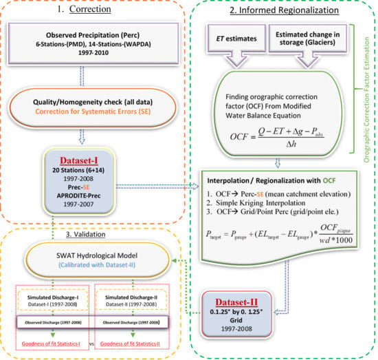
The informed spatial regionalization of the precipitation data in the UIB involves basically three main processes: (1) Pre-processing of the raw precipitation data (quality check & correction of systematic errors), (2) estimation of a catchment-specific orographic correction factor (OCF) or precipitation laps rate (PLR) by “Doing Hydrology backward”, and (3) stepwise interpolation/regionalization (OCF adjustment of observed precipitation at catchment mean elevation, followed by simple kriging and finally an OCF readjustment of the interpolated data to target grid-average/point elevation). These three steps are described in detail in the subsequent sub-sections.
3.2.1. Correction of Systematic Errors
The first step consists of the correction of systematic errors in the raw uncorrected precipitation data available for the UIB. This task serves to remove any systematic errors in precipitation measurements and to correct the possible precipitation under catch during snowfall, particularly, under windy conditions. For this purpose, different methods recommended by the World Meteorological Organization (WMO) were reviewed, and the method of Reference [78] was selected as it requires less observed parameters and has also previously been applied in the study region. It should be noted though that, prior to application of the corrections for systematic errors, the observed precipitation dataset was checked for inhomogeneity and outliers. This correction method employs Equations (1) and (2) to account for wind-induced errors, wetting losses, evaporation losses and trace amounts. The equations suggested by the method in References [78,79] are as follows:
where Pc is the ‘corrected’ precipitation; Pm, the measured gauge value; ΔPw, the wetting losses; ΔPe, evaporation losses; ΔPt, trace amount; and K, the adjustment coefficient due to wind-induced errors, for which CR is the catch ratio (%), defined as a function of wind speed. The values of ΔPw, ΔPe, ΔPt and CR suggested by References [78,79], used in this study, are given in Table 3.
For allocating values for ΔPw, ΔPe, ΔPt and CR in the calculations, the precipitation was considered during (1) the winter months (DJF) as Snow, (2) the summer months (JJO) as Rain, and (3) spring and autumn (MAM and SON) as Mixed.
3.2.2. Estimating the “Orographic Correction Factor” (OCF) by Doing Hydrology Backward (DHB) plus Interpolation (Informed Regionalization (IR))
• General approach
The “Orographic correction factor” (OCF) is calculated based on the rearranged “hydrological/water balance equation” (Equations (6) and (7)). The calculation utilizes five data variables, out of which data for three variables: mean annual catchment precipitation, mean annual catchment discharge, and catchment and gauge point elevation were available, whereas the other two variables required, catchment mean annual change in glacier storage (mm) and catchment mean annual actual-evapotranspiration, were estimated based on the relevant literature and gridded data products. The final OCF is through an adjusted variant of the “equation-based version”, which was computed based on the hydrological modeling calibration, until the simulated mass balance came to an acceptable match to the observed mass balances.
• The hydrological/water balance equation
The hydrological/water balance equation [80] is as follows:
where Qt is the total volume of water discharging from a catchment (per specified time period), and is equal to the volume of water entering the catchment as true precipitation (P) minus a change in storage and losses from the system. The latter comprise of losses by actual evapotranspiration (ET), aquifer/ground-water recharge (Gw) and losses or gains of glacier ice volume (∆g).
As the losses Gw, may be minimal in comparison to the total discharge especially for large mountainous catchments and at an inter-annual time step, the above equation can be simplified to:
or
By assuming the true aerial precipitation Ptrue to be equal to the observed precipitation Pobs plus the orographic under/overestimation OCF, one gets:
Basically, the OCFT represents the under- or over estimation by the low-altitude average observed precipitation of the true areal precipitation over the gauged catchment.
The OCF per unit elevation, OCFplapse, is found by dividing OCF by the difference Δh in mean elevation of the catchment and the observation network, i.e., by arranging Equations (6), one gets
One can also define the orographic correction multiplicative factor, , by dividing the true precipitation Ptrue by the observed precipitation Pobs:
In the presence of the water discharge data from the system (Q), observed precipitation (Pobs) and elevation (Δh), only estimates of glacier mass balance (Δg) and evapotranspiration (ET) are required to calculate the OCF for each gauged catchment. The values for these parameters are estimated based on available literature values for gridded data sets for glacier mass balance and actual evapotranspiration, as detailed in the subsequent sub-chapters.
• Glacier mass balance (Δg) estimates
Estimating the glacier storage change (∆g) in the different catchments of the UIB is a very difficult and uncertain task, because no consensus could be found within the available literature on either the amount of decrease in most of the southern and eastern parts or the possible increase (or decrease) in the northern or western parts of the HKH region.
Much of the UIB spans over different mountain ranges, out of which the watersheds of Hunza, Shigar, and Shyok span the Karakoram mountains; Gilgit watershed covers the north-eastern Hindu Kush, while four watersheds (Astore, Shingo, Zanskar, and remaining part of the UIB upstream of Kharmong) are located across the Western Greater Himalayas. Therefore, the mass balance of the glaciers in these mountain ranges and the watersheds spanning over them is as diverse as their hydro-climatic regimes are different and hard to find out.
Although the decreases or increases suggested by different studies may differ notably, many of the recent studies are consistent in pointing out a decreasing trend in the eastern and central Himalayas and a steady or slightly increasing trend in the Karakorum and other adjoining ranges in the north and west. These claims are supported by other hydro-climatic factors, such as an increase in observed precipitation for winter and summer [81,82], the Karakorum anomaly validated by Reference [83], with the findings of a positive mass balance for the central Karakoram glaciers and less summer flows, in spite of a precipitation increase [82].
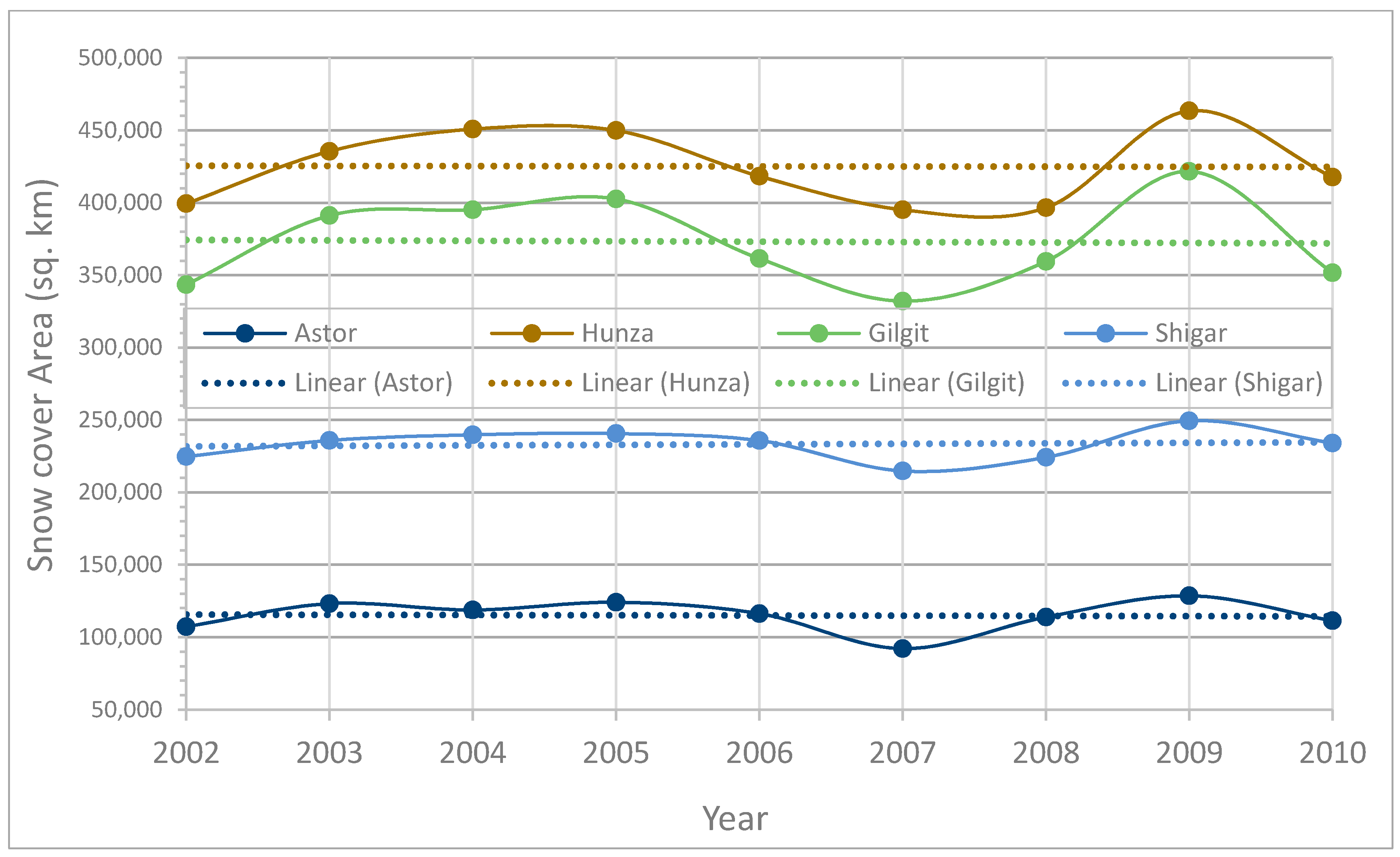
The snow cover change over different catchments in the UIB (Figure 2), derived based on statistics available at “HKH Snow Cover-web application” hosted by ICIMOD, is also in conformity with the claims of a stable to positive glacier mass balance in the Karakorum. Other recent studies [32,82,83,84,85,86,87,88] indicate similar trends of glacier mass balance in the region. These trends of glacier mass balance are summarized for a few recent studies in Table 4.
Despite these agreements on the trends of net glacier mass change, there are huge differences between the studies regarding their absolute amounts. These uncertainties are further exacerbated by the fact that different authors used different source data, different assessment periods and different procedures. To avoid some of these complexities, one of the recent studies, i.e., Reference [83], which is also in line with others (e.g., References [82,87,88] etc.), is selected as a reference for glacier mass balance in different parts of the UIB, with the major results as outlined below:
- (a)
- (b)
- The Gilgit watershed, though spanning over the northern end of the Hindukush range (bordering the western Karakoram) is assigned the same value of +0.09 mwe year−1, because, as reported by Reference [82], this watershed has more similarities with the climatic regime of the Karakoram region (Hunza basin), rather than the rest of the Hindukush area.
- (c)
- For the Shyok river basin, a snow cover change of +0.11 mwe year−1 is assumed based on the value given by Reference [83] for the east Karakorum.
- (d)
- For the region covered by the Astor basin and the parts of UIB downstream of Kharmong, except the aforementioned tributary catchments, the selection is not straight forward, as some of the above studies claim a constant/slight increase in snow cover area in this region (e.g., Reference [82]), while others suggest a negative mass balance. Therefore, for the current study, the glacier mass balance in this region is taken as neutral, with no increase or decrease.
- (e)
- For the parts of UIB, upstream of Kharmong, which have experienced a consistent decrease in snow/glacier cover, according to most of the literature, a value of −0.45 mwe year−1 is assigned, based on the mean mass balance value [83] for the Spiti-Lahaul region.
The glacier mass balance amounts selected above for the different regions are converted from meters water equivalent per year (mwe year−1) to glacier storage changes in millimeter depth (mm) (Table 5), before using them in the calculation for the orographic correction factor.
• Evapotranspiration (ET) estimates:
Observed actual evapotranspiration (ET) data are a very rare commodity, even in easy-to-access areas. This holds also for the UIB, where there are not much direct measurements available [72]. For ET-estimations, especially in the UIB and elsewhere too, most of the previous studies relied on either temperature-based empirical relationships or, in more recent times, on calculated algorithms utilizing data with different combinations of various ground- or sensors-based observed hydro-climatic variables [90,91,92,93,94]. A few studies suggested to address the uncertainties in the different ET-estimates by blending them to acquire an average trend (e.g., Reference [72]).
Despite some improvements in the estimation techniques or the data used in these studies, the uncertainties in ET-estimates are huge, especially for areas like the UIB, where the other available data also have huge uncertainties. For the UIB, most of the gridded evapo-transpiration products show very high average annual ET values, which appear unrealistic when compared to the observed annual precipitation over the UIB of 350–400 mm year−1 (~367 mm year−1 based on the observed and APHRODITE precipitation data, given in and Table 7 later).
The mean annual ET values, proposed by most of the available gridded products such as the “Global Average Annual Evapotranspiration, 1950–2000”, data hosted at Databasin.org [95], have very high average ETs over different catchments of UIB (~300–400 mm year−1). Similarly, the ET values proposed by Immerzeel et al. [72], based on four different available ET products, have a mean annual value of 359 ± 107. These proposed mean annual ET values are probably too high to leave any water left for runoff generation.
The reason is that in the high-elevation mountainous catchments of the HKH, evapotranspiration only plays a minor role in the overall water balance and is generally less than 10% of the total hydrological budget [96]. This also applies to the UIB where only the lower-altitude area may have higher ET contributions, while the high elevation sub-catchments may have only minor annual ET due to their low average temperatures. For example, in the Hunza basin of the UIB, Garee et al. [97], reported a model ET equal to 18% of the precipitation, indicating even lower ET in the higher altitude catchments. Therefore, in UIB, which is also a high mountainous basin and has a mean annual water discharge of around 462 mm year−1, the ET in UIB should not amount to such high values, almost equal to the observed runoff.
To solve these issues, ET products with relatively lower values were evaluated. One such ET data is the Esri_hydro “Average Annual Evapotranspiration” [98], which is based on the MOD16 Global Evapotranspiration Product, and is derived from MODIS-satellite imagery by a team of researchers at the University of Montana, has comparatively lower ET-estimates, which better match the recommended values of Bookhagen and Burbank [96] or the ET-values reported by Garee et al. [97]. The MOD16-ET-data have a good resolution of 1 km2 and are available over the period 2000–2011. For this reason, they are used here as reference-ET in the OCF-calculation, and their values are also listed for the different UIB-catchments in Table 5.
3.2.3. Regionalization Procedure—Step-Wise Interpolation
The gauge-station precipitation records and the APHRODITE-precipitation were processed separately. The gauge-station-observed precipitation time series, after correction for systematic errors and quality check, was interpolated to 0.125° by 0.125° grid in three steps.
In the first step of this “regionalization/stepwise interpolation” process, all the point-observed data are adjusted for the mean catchment elevation as:
where Ptarget is the precipitation at target elevation (mm); Pgauge is the precipitation recorded at the gauge station (mm); ELtarget is the elevation at the target point/grid; ELgauge is the elevation at the gauge station; wd is the average annual number of wet days; and OCFplapse (Equation (8)) is the orographic correction factor, in terms of the precipitation lapse rate, for the catchment.
In the second step, the data adjusted at the mean catchment elevation is then interpolated using “Simple Kriging” [59], to a 0.125° by 0.125° grid as well as SWAT-Model sub-basin centroids.
In the third step, the interpolated data are readjusted from the mean catchment elevation to the grid elevation, using Equation (9).
For the APHRODITE data, the correction for the orographic effect was done using the multiplicative correction factor OCFmultiplicative (Equation (8)), prior to interpolation using “Simple Kriging” [59], to a 0.125° by 0.125° grid as well as SWAT-Model sub-basin centroids, as discussed below.
3.2.4. Validation of Estimates Precipitation by Means of the SWAT Hydrological Model
• SWAT Model Description
The Soil and Water Assessment Tool (SWAT) is a hydrological model developed for the US Department of Agriculture (USDA), Agricultural Research Service (ARS) by Dr. Jeff Arnold and collaborators. The SWAT-model is a continuous time (long-term yield), process-based semi-distributed model, capable of simulating hydrological processes in river basins/watersheds, based on specific information pertaining to the watershed, such as weather/climate, topography, soil properties, land cover, land use and management practices [99,100]. In the SWAT-model, a main river basin or watershed is partitioned into several sub-units called sub-basins draining the tributaries into the stream network and the river-system. These sub-basins are further divided into a series of smaller units, the co-called hydrological response units (HRUs), which are spatial uniform units, each representing a unique combination of soil, land-use and slope. The calculation and simulation of the various hydrological components is based on the solution of the fundamental water balance equation (Equation (3)), wherefore these components which may include, in addition, sediment yield and agricultural nutrients, are first evaluated for each HRU and then routed and aggregated for the subbasin and finally for the watershed.
In the current study, “ArcSWAT-2012”, which is an ArcGIS-ArcView extension and graphical user input interface for the SWAT-model, is used. The SWAT-input data employed here include: a void-filled, and hydrologically conditioned, 3 arc-seconds (=90 × 90 m2)—spatial resolution digital elevation model (DEM) from Hydro-SHEDS [101], FAO-UNESCO global soil map [102] (FAO-UNESCO Digital Soil Map of the World, 2007) and “Global Land Cover Characterization (GLCC) at 1 km spatial resolution (U.S. Geological Survey [103]. During the watershed delineation process, the study area with a size of 165611 km2 was configured into 173 sub-basins, divided further into a total of 2825 discrete HRUs.
Because the goal of the use of the SWAT model is to ascertain and validate the precipitation IR-method of the previous section, weather/climate forcing on the model comprises two precipitation datasets: (1) gauge-station-observed precipitation (1997–2008); and (2) corrected & regionalized precipitation (1997–2008). In both cases, the temperature data required as inputs to the SWAT model are the same.
• Model Calibration and Validation setup
The SWAT model was calibrated and validated against daily discharge individually for each of its five major tributaries (Hunza, Gilgit, Astor, Shigar and Shyok rivers), for parts of UIB (except the tributaries) inside Pakistan’s boundary and for the UIB (situated in India China and Nepal) covering the area upstream of the Kharmang gauge station. In cases of catchments, where inflow from the upstream catchment had to be accounted for, the observed discharge was used as inflow.
The Sequential Uncertainty Fitting SUFI-2 algorithm [104] of the SWAT-CUP program [104] was used for parameter optimization during the calibration process.
For the performance evaluation of calibration/validation results, the “goodness of fit” statistics including the coefficient of determination (R2), Nash Sutcliff efficiency (NS) and Percentage bias (PBIAS) are used, which assess the simulated hydrological responses against the observed flow data.
4. Results and Discussion
4.1. Construction of Orographically-Corrected Precipitation Datasets
The selected and finalized values for the glacier mass balances Δg and the actual evapotranspiration ET (Table 5) are utilized in Equations (7) and (8) to derive the two kinds of catchment-specific orographic correction factors (OCF), namely, the multiplicative correction factor OCFmultiplicative and the additive correction factor OCFlapse (representing the precipitation lapse rate per 1000 m elevation change). The former are derived for the uncorrected raw precipitation for both gauge- and APHRODITE-data sets, while the latter is calculated only for the gauge station records, after correction for systematic errors.
The additive correction factor OCFlapse is applied at all the elevation ranges, wherefore it is assumed that the precipitation increases uniformly with elevation and the correction factor is constant throughout the year. To further improve the regionalization, and with more data available, it would also be possible to apply a range of catchment- or season-specific OCF’s to generate the desired vertical or temporal regimes of precipitation to match any empirical distributions of precipitation intensities in different elevation zones or seasons.
4.2. True Areal Precipitation and OCF’s
The details of the annual input data and the results obtained for the different OCF’s for the various UIB catchments are listed in Table 6 and Table 7. The findings are in total conformity with conclusions of many previous studies, which claim that the gauge-based data as well as the remotely sensed precipitation products are unable to represent the true areal precipitation in the UIB [11,12,13,14].
• Spatial distribution of orographically-corrected precipitation datasets
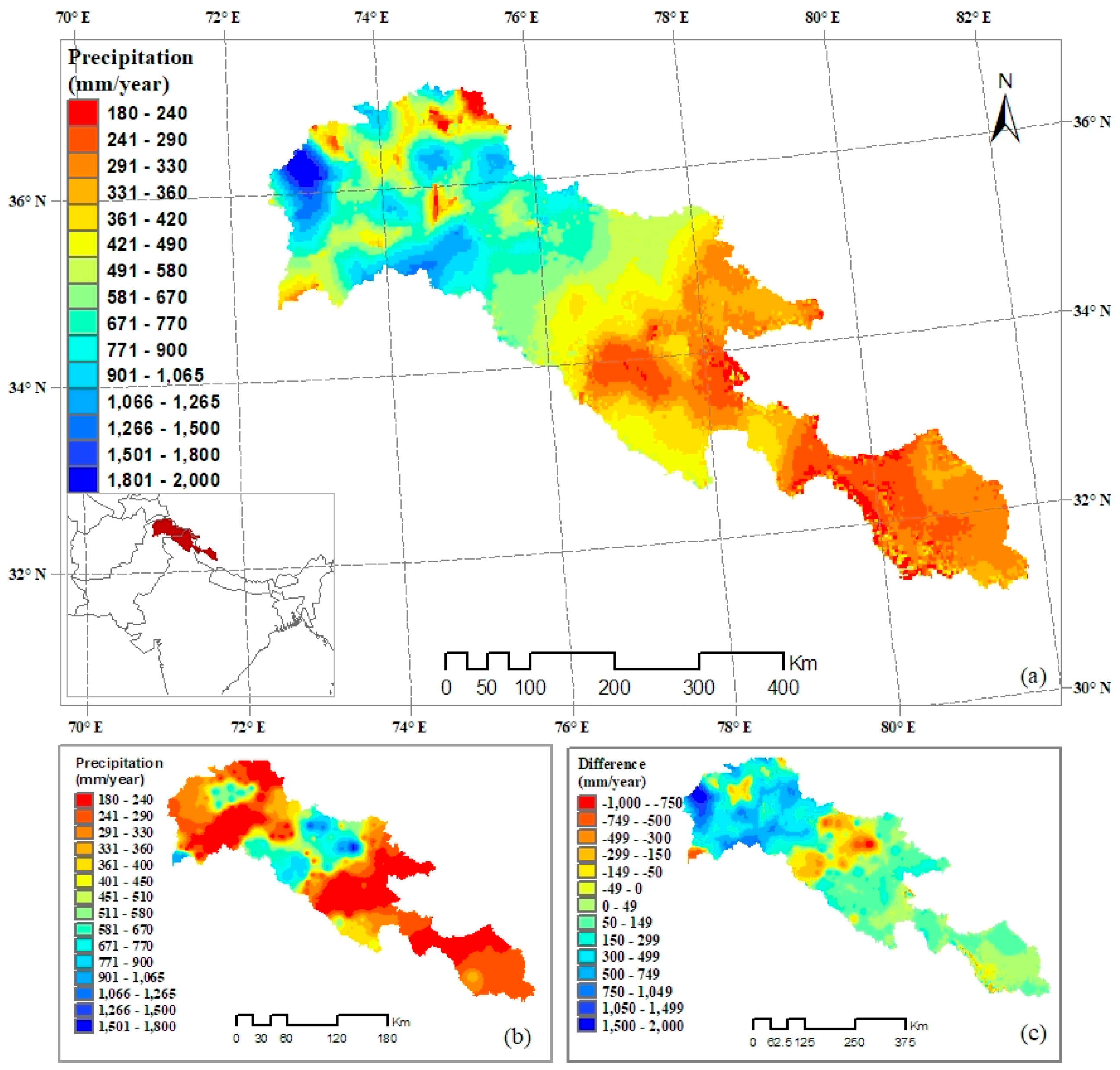
The final gridded precipitation generated after the step-wise interpolation to the 0.125° × 0.125° grid by simple Kriging, followed by the appropriate elevation correction with OCFlapse at the target points is shown in the map of Figure 3a. Obviously the application of the elevation OCFlapse, while remaining true to the originally estimated mean precipitation for each catchment (Table 6), has added some diversity, as it produces a spatially distributed precipitation over UIB and its catchments with elevation-dependent lapse gradients. For comparison, the observed/APHRODITE interpolated precipitation distribution as well the difference between the two are shown in Figure 3b,c, respectively, with the latter witnessing clearly the underestimations of the observed/APHRODITE precipitation in most areas of the UIB.
Overall, the corrected and regionalized precipitation in Figure 3a, reveals outstanding patterns of spatial and orographic distributions. Our results match well with those of recent available studies of precipitation with respect to intensities, horizontal and vertical distribution as well as regional trends in the UIB [23], although our precipitation values are slightly lower as [23], because we have assumed a smaller ET rate over the UIB. The spatial distribution and trends obtained here are also in conformity with others (e.g., References [19,20,24,30]), such that over the extent of the UIB, the highest average annual precipitation is found in the west, due to the prevailing midlatitude western disturbances. The monsoonal contributions over the UIB are also in accordance with results of (e.g., References [20,24,28]), such that they act mostly in the southern fringes of the western Himalayas in the UIB, but are waning in the north and west (Figure 3a).
Table 6 shows that the mean OCF-corrected precipitation over the UIB for the 1999–2008 period has a value of ~608 mm/year, which is considerably higher than the average uncorrected gauge station and APHRODITE measured annual precipitation of 367 mm/year, (i.e., the latter is underestimated by ~166%). For some catchments in the UIB (Gilgit and Shyok), these underestimations of the true precipitation are even in excess of 300%.
The strong relation between the topographic altitude and precipitation amount [20], is also well accounted for by our results, with very high precipitation over the elevated zones of the Gilgit and Astore basins, and comparatively weaker orographic influences in the rain-shadow regions in the north or east. Resultantly, the north-western parts of the UIB, which lie inside Pakistan’s boundary, show the highest mean annual precipitation, especially over the Gilgit and Astor river catchments, of above 2000 mm/year. There is a gradual decrease in the mean annual precipitation to the north of these two catchments, with Hunza and Shigar having lower precipitation. A similar decreasing precipitation gradient is witnessed in the west-east direction of the UIB, so that the lowest mean precipitation is witnessed in the easternmost parts of the basin.
4.3. Validation of the Corrected Precipitation against SWAT-Simulated Discharge
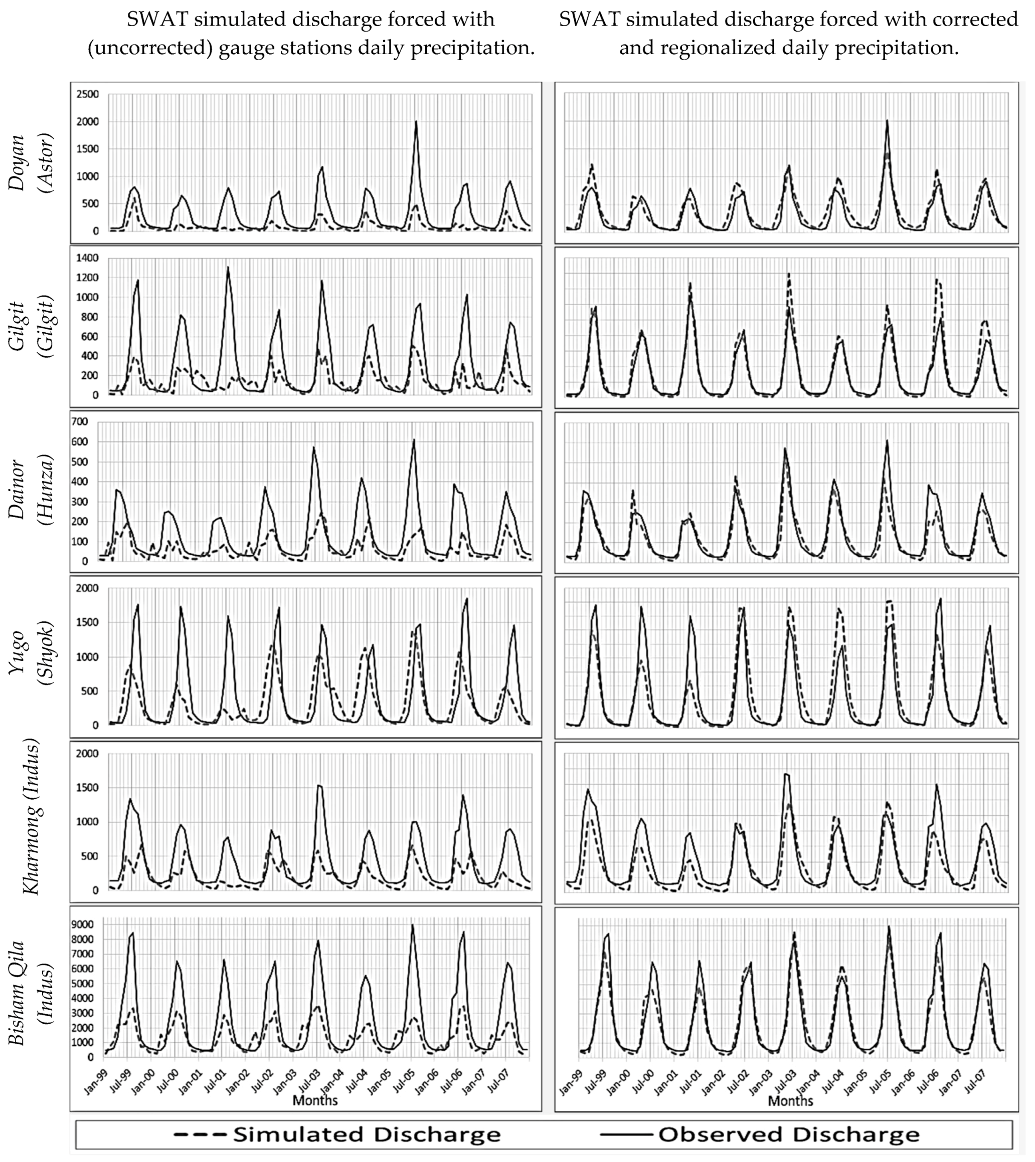
To validate the final product of the proposed precipitation correction and regionalization method, the SWAT hydrological model was forced with the two different precipitation data series: (1) observed, gauge- and (2) orographically-corrected & regionalized precipitation, both for the time period 1999–2008.
The goodness of fit statistics of the SWAT-simulated discharges for the two categories of precipitation input data are listed in Table 8, while the comparisons of simulated and observed discharges (hydrographs) are presented in Figure 4.
That is why, when forced with corrected and regionalized precipitation, the SWAT-simulated daily discharges match the observed discharges much better, and this holds for all the monitoring points across the various tributary catchments (Figure 4).
The goodness of fit statistics (Table 8) also show drastic improvements over those of the simulations forced with uncorrected gauge station precipitation series. For all the monitoring points in the UIB, the R2 are above 0.69 and go as high as 0.89. The NS-values are also on the higher side and range between 0.69 and 0.89. Overall, a R2 of 0.86 and a NS of 0.85 is obtained at the basin outlet, which can be considered as very good results, especially for hydrological simulations carried out at a daily time step. Furthermore, the PBIAS-values of the simulated discharges are also much lower than those of the first SWAT-simulations category, with maximum positive and negative biases of 12.4% and −19.7%., respectively.
These results verify clearly the validity of the adopted methodology of precipitation correction and informed regionalization by accounting for orographic influences and regional patterns at the gauged catchments scale for use in hydrological modeling studies.
4.4. Merits and Limitation of the Proposed Method and Regionalized Data
We will assess our precipitation data in comparison of the available precipitation products as well as check the comparative strengths and weaknesses of our proposed method.
Currently, various gridded precipitation data sets are available for HKH. They include satellite data products, such as the TRMM 3B42 product, rain-gauge based collections (i.e., APRHODITE, CRU, GPCC), combined satellite and rain gauge climatology (GPCP), reanalysis products (i.e., ERA-Interim) etc. Although all these data sets are reasonably suitable for hydro-climatic studies at a regional scale; owing to the complex orography of the UIB region and to the co-action of different hydro-climatic regimes (which affect the amounts, spatial patterns and the seasonality of precipitation), neither the sparse observed station data (or the gridded data products based on them) nor the sensors-based data, fully represents the precipitation regime of the region [11,12,13,14].
This has led many researchers to find ways to assess methods for precipitation correction that may lead to a more realistic water balance [21] in many basins and have also compelled a number of hydrological studies in the UIB region to use, in addition to the observed station data, a variety of other reference climate data from different sources, either directly or with prior modifications and adjustments (e.g., TRMM Data [22]; modified APHRODIT [23], modified WFDEI data [13] or modified observed data through reverse hydrology [72] etc.). All these data sets have been produced through reasonably complex methodology or possibly have under or overestimated precipitation magnitudes. For example, the precipitation estimates by Reference [72] have utilized evapotranspiration values which appear to be higher than the realistic (or reported) limits.
To avoid these downsides, we have tried to devise a method which may not only be less complex, but also produce precipitation data capable of capturing the prevalent spatial patterns and orographic influences in UIB, at least at gauged catchment scale. The proposed method is not only guided by realistic or reported glacier mass-balance, evapotranspiration and orographic influences, but also producing precipitation estimates that are able to close the water balance in UIB.
Although our results clearly suggest the validity of the proposed method, the method is not without limitations. The spatial patterns of precipitation are based on a fixed correction factor for each gauged catchment, and hence, are unable to provide explicitly distributed precipitation, as the single orographic correction factor applied per catchment cannot compensate for the variation in orographic influences inside a catchment. Similarly, the estimated precipitation inherited uncertainties attached to the glacier-mass balance estimates as well as ET data used.
5. Conclusions
In this study, we addressed the underestimation and low representation of the high-altitude precipitation by the available gauge-based records by doing hydrology backwards in conjunction with available cryosphere and hydro-climatic information. Despite certain uncertainties, our precipitation estimates are not only accounting for the orographic influences, but also for the glacial mass balance across different catchments of the UIB. The corrected and regionalized data is therefore making it possible for hydrological investigations to properly close the water balance, which is unlikely to be achieved with the available observed gauge-based or gridded precipitation datasets.
The estimations of the horizontal and vertical distributions as well as the magnitudes and intensities of the precipitation achieved by our correction and informed regionalization approach are matching well with those reported in the literature. Furthermore, the SWAT-hydrological simulations (doing hydrology backwards) using the corrected precipitation data match the observed flow in the UIB even better than our expectations.
Thus, whereas the SWAT-hydrological simulations using uncorrected observed precipitation show poor fit with the observed discharges, with values for R2 and NSE not greater than 0.77 and 0.41, respectively, and huge underestimations of the flows across all the investigated catchments of the UIB, with PBIAS-values of up to −72.87%, the situation is much improved when using the corrected precipitation datasets in the model. In these cases, simulated flows match the observed flows very well, with R2 ranging between 0.69 and 0.89, with a similar range for the NSE and, last but not least, small PBIAS-values ranging between 12.4% and −19.7%.
The results of the present study show that major improvements in rainfall estimations in poorly gauged, high mountain regions, like the UIB, can be achieved by combining classical orographic correction methods with knowledge of the regional hydro-meteorology and glacier mass balance at the gauged catchment levels (in case of glaciated catchments) and validating such a methodology by an additional hydrological model, in order to remove inconsistencies in and to close the hydrological water balance (doing backward hydrology). This multistep approach is not only less demanding in terms of computational or human resource requirements than the methods involving advanced atmospheric physics or geostatistics, but can considerably improve the quality and representativeness of the precipitation data at a gauged catchment scale.
Author Contributions
Conceptualization, A.J.K.; Formal analysis, A.J.K.; Investigation, A.J.K.; Methodology, A.J.K.; Resources, M.K.; Supervision, M.K.; Validation, A.J.K.; Writing—original draft, A.J.K.; Writing—review & editing, M.K.
Funding
This research received no external funding.
Acknowledgments
We acknowledge provision of data by the following sources: Hydro-Shed-3sec GRID: Conditioned DEM, courtesy of the U.S. Geological Survey; FAO-UNESCO Soil Map of the World, version 3.6; courtesy of the Food and Agriculture Organization of the United Nations. FAO GEONETWORK, 2007; GLCC—Global Land Cover Characteristics Data Base, Version 2.0; courtesy of the U.S. Geological Survey, USGS EROS Data Centre; and Water and Power Development Authority (WAPDA) and Pakistan Meteorological Department (PMD), for their exchange of the valuable hydrological and climate data to complete my research.
Conflicts of Interest
The authors declare no conflict of interest.
Appendix A
Figure A1.
Vertical and horizontal meteorological and cryspheric regimes in UIB (modified from Hewitt 2007).
Figure A1.
Vertical and horizontal meteorological and cryspheric regimes in UIB (modified from Hewitt 2007).

References
- Duncan, M.R.; Austin, B.; Fabry, F.; Austin, G.L. The effect of gauge sampling density on the accuracy of streamflow prediction for rural catchments. J. Hydrol. 1993, 142, 445–476. [Google Scholar] [CrossRef]
- Singh, P.; Jain, S.K.; Kumar, N. Estimation of Snow and Glacier-Melt Contribution to the Chenab River, Western Himalaya. Mt. Res. Dev. 1997, 17, 49. [Google Scholar] [CrossRef]
- Andréassian, V.; Perrin, C.; Michel, C.; Usart-Sanchez, I.; Lavabre, J. Impact of imperfect rainfall knowledge on the efficiency and the parameters of watershed models. J. Hydrol. 2001, 250, 206–223. [Google Scholar] [CrossRef]
- Kobold, M.; Sušelj, K. Precipitation forecasts and their uncertainty as input into hydrological models. Hydrol. Earth Syst. Sci. 2005, 9, 322–332. [Google Scholar] [CrossRef] [Green Version]
- Leander, R.; Buishand, T.A.; van den Hurk, B.J.J.M.; de Wit, M.J.M. Estimated changes in flood quantiles of the river Meuse from resampling of regional climate model output. J. Hydrol. 2008, 351, 331–343. [Google Scholar] [CrossRef]
- Rueland, D.; Larrat, V.; Guinot, V. A Comparison Oftwo Conceptual Models for the Simulation of Hydro-Climatic Variability Over 50 Years in a Large Sudano-Sahelian Catchment; International Association of Hydrological Sciences: Wallingford, UK, 2010. [Google Scholar]
- Moulin, L.; Gaume, E.; Obled, C. Uncertainties on mean areal precipitation: Assessment and impact on streamflow simulations. Hydrol. Earth Syst. Sci. 2009, 13, 99–114. [Google Scholar] [CrossRef] [Green Version]
- Liu, Y.B.; de Smedt, F. WetSpa Extension, A GIS-Based Hydrologic Model for Flood Prediction and Watershed Management: Documentation and User Manual; Vrije Universiteit Brussel: Brussel, Belgium, 2004. [Google Scholar]
- Obled, C.; Wendling, J.; Beven, K. The sensitivity of hydrological models to spatial rainfall patterns: An evaluation using observed data. J. Hydrol. 1994, 159, 305–333. [Google Scholar] [CrossRef]
- Rodda, J.C. Report on precipitation. Int. Assoc. Sci. Hydrol. Bull. 1971, 16, 37–47. [Google Scholar] [CrossRef]
- Yatagai, A.; Kamiguchi, K.; Arakawa, O.; Hamada, A.; Yasutomi, N.; Kitoh, A. APHRODITE: Constructing a Long-Term Daily Gridded Precipitation Dataset for Asia Based on a Dense Network of Rain Gauges. Bull. Am. Meteor. Soc. 2012, 93, 1401–1415. [Google Scholar] [CrossRef]
- Palazzi, E.; Filippi, L.; von Hardenberg, J. Insights into elevation-dependent warming in the Tibetan Plateau-Himalayas from CMIP5 model simulations. Clim. Dyn. 2017, 48, 3991–4008. [Google Scholar] [CrossRef]
- Wijngaard, R.R.; Lutz, A.F.; Nepal, S.; Khanal, S.; Pradhananga, S.; Shrestha, A.B.; Immerzeel, W.W. Future changes in hydro-climatic extremes in the Upper Indus, Ganges, and Brahmaputra River basins. PLoS ONE 2017, 12, e0190224. [Google Scholar] [CrossRef] [PubMed]
- Palazzi, E.; von Hardenberg, J.; Provenzale, A. Precipitation in the Hindu-Kush Karakoram Himalaya: Observations and future scenarios. J. Geophys. Res. Atmos. 2013, 118, 85–100. [Google Scholar] [CrossRef] [Green Version]
- Singh, P.; Kumar, N. Effect of orography on precipitation in the western Himalayan region. J. Hydrol. 1997, 199, 183–206. [Google Scholar] [CrossRef]
- Dhar, O.N.; Rakhecha, P.R. The effect of elevation on monsoon rainfall distribution in the central Himalayas. In Monsoon Dynamics; Lighthill, M.J., Pearce, R.P., Eds.; Cambridge University Press: New York, NY, USA, 1981; pp. 253–260. [Google Scholar]
- Dahri, Z.H.; Ludwig, F.; Moors, E.; Ahmad, B.; Khan, A.; Kabat, P. An appraisal of precipitation distribution in the high-altitude catchments of the Indus basin. Sci. Total Environ. 2016, 548–549, 289–306. [Google Scholar] [CrossRef] [PubMed] [Green Version]
- Pang, H.; Hou, S.; Kaspari, S.; Mayewski, P.A. Influence of regional precipitation patterns on stable isotopes in ice cores from the central Himalayas. Cryosphere 2014, 8, 289–301. [Google Scholar] [CrossRef] [Green Version]
- Hewitt, K. Glacier Change, Concentration, and Elevation Effects in the Karakoram Himalaya, Upper Indus Basin. Mt. Res. Dev. 2011, 31, 188–200. [Google Scholar] [CrossRef]
- Wake, C.P. Glaciochemical Investigations as a Tool for Determining the Spatial and Seasonal Variation of Snow Accumulation in the Central Karakoram, Northern Pakistan. Ann. Glaciol. 1989, 13, 279–284. [Google Scholar] [CrossRef] [Green Version]
- Valéry, A.; Andréassian, V.; Perrin, C. Regionalization of precipitation and air temperature over high-altitude catchments—Learning from outliers. Hydrol. Sci. J. 2010, 55, 928–940. [Google Scholar] [CrossRef]
- Immerzeel, W.W.; Droogers, P.; de Jong, S.M.; Bierkens, M.F.P. Large-scale monitoring of snow cover and runoff simulation in Himalayan river basins using remote sensing. Remote Sens. Environ. 2009, 113, 40–49. [Google Scholar] [CrossRef]
- Lutz, A.F.; Immerzeel, W.W.; Kraaijenbrink, P.D.A.; Shrestha, A.B.; Bierkens, M.F.P. Climate Change Impacts on the Upper Indus Hydrology: Sources, Shifts and Extremes. PLoS ONE 2016, 11, e0165630. [Google Scholar] [CrossRef] [PubMed]
- Ali, K.F.; de Boer, D.H. Spatial patterns and variation of suspended sediment yield in the upper Indus River basin, northern Pakistan. J. Hydrol. 2007, 334, 368–387. [Google Scholar] [CrossRef]
- Internat. Centre for Integrated Mountain Development. The Status of Glaciers in the Hindu Kush-Himalayan Region; Bajracharya, S.R., Shrestha, B., Eds.; International Centre for Integrated Mountain Development: Kathmandu, Nepal, 2011. [Google Scholar]
- RGI Consortium. Randolph Glacier Inventory 5.0. A Dataset of Global Glacier Outlines: Version 5.0; GLIMS Technical Report; Global Land Ice Measurements from Space: Boulder, CO, USA, 2015. [Google Scholar] [CrossRef]
- Tahir, A.A.; Chevallier, P.; Arnaud, Y.; Ahmad, B. Snow cover dynamics and hydrological regime of the Hunza River basin, Karakoram Range, Northern Pakistan. Hydrol. Earth Syst. Sci. 2011, 15, 2275–2290. [Google Scholar] [CrossRef] [Green Version]
- Bookhagen, B.; Burbank, D.W. Topography, relief, and TRMM-derived rainfall variations along the Himalaya. Geophys. Res. Lett. 2006, 33, 21. [Google Scholar] [CrossRef]
- Ali, S.; Li, D.; Congbin, F.; Khan, F. Twenty first century climatic and hydrological changes over Upper Indus Basin of Himalayan region of Pakistan. Environ. Res. Lett. 2015, 10, 14007. [Google Scholar] [CrossRef] [Green Version]
- Hasson, S.U. Future Water Availability from Hindukush-Karakoram-Himalaya upper Indus Basin under Conflicting Climate Change Scenarios. Climate 2016, 4, 40. [Google Scholar] [CrossRef]
- Karim, A.; Veizer, J. Water balance of the Indus River Basin and moisture source in the Karakoram and western Himalayas: Implications from hydrogen and oxygen isotopes in river water. J. Geophys. Res. 2002, 107, 190. [Google Scholar] [CrossRef]
- Hewitt, K. Tributary glacier surges: An exceptional concentration at Panmah Glacier, Karakoram Himalaya. J. Glaciol. 2007, 53, 181–188. [Google Scholar] [CrossRef]
- Archer, D. Contrasting hydrological regimes in the upper Indus Basin. J. Hydrol. 2003, 274, 198–210. [Google Scholar] [CrossRef]
- Khan, F.; Pilz, J.; Amjad, M.; Wiberg, D.A. Climate variability and its impacts on water resources in the Upper Indus Basin under IPCC climate change scenarios. IJGW 2015, 8, 46. [Google Scholar] [CrossRef]
- Khan, F.; Pilz, J.; Ali, S. Improved hydrological projections and reservoir management in the Upper Indus Basin under the changing climate. Water Environ. J. 2017, 31, 235–244. [Google Scholar] [CrossRef]
- Kirchner, J.W. Catchments as simple dynamical systems: Catchment characterization, rainfall-runoff modeling, and doing hydrology backward. Water Resour. Res. 2009, 45, 2135. [Google Scholar] [CrossRef]
- Teuling, A.J.; Lehner, I.; Kirchner, J.W.; Seneviratne, S.I. Catchments as simple dynamical systems: Experience from a Swiss prealpine catchment. Water Resour. Res. 2010, 46, 305. [Google Scholar] [CrossRef]
- Creutin, J.D.; Delrieu, G.; Lebel, T. Rain Measurement by Raingage-Radar Combination: A Geostatistical Approach. J. Atmos. Ocean. Technol. 1988, 5, 102–115. [Google Scholar] [CrossRef] [Green Version]
- Beek, E.G.; Stein, A.; Janssen, L.L.F. Spatial variability and interpolation of daily precipitation amount. Stoch. Hydrol. Hydraul. 1992, 6, 304–320. [Google Scholar] [CrossRef]
- Kurtzman, D.; Kadmon, R. Mapping of temperature variables in Israel: A comparison of different interpolation methods. Clim. Res. 1999, 13, 33–43. [Google Scholar] [CrossRef]
- Shen, S.S.P.; Dzikowski, P.; Li, G.; Griffith, D. Interpolation of 1961–1997 Daily Temperature and Precipitation Data onto Alberta Polygons of Ecodistrict and Soil Landscapes of Canada. J. Appl. Meteor. 2001, 40, 2162–2177. [Google Scholar] [CrossRef]
- Kyriakidis, P.C.; Kim, J.; Miller, N.L. Geostatistical Mapping of Precipitation from Rain Gauge Data Using Atmospheric and Terrain Characteristics. J. Appl. Meteor. 2001, 40, 1855–1877. [Google Scholar] [CrossRef]
- Buytaert, W.; Celleri, R.; Willems, P.; Bièvre, B.D.; Wyseure, G. Spatial and temporal rainfall variability in mountainous areas: A case study from the south Ecuadorian Andes. J. Hydrol. 2006, 329, 413–421. [Google Scholar] [CrossRef] [Green Version]
- Stahl, K.; Moore, R.D.; Floyer, J.A.; Asplin, M.G.; McKendry, I.G. Comparison of approaches for spatial interpolation of daily air temperature in a large region with complex topography and highly variable station density. Agric. For. Meteorol. 2006, 139, 224–236. [Google Scholar] [CrossRef]
- Daly, C. Guidelines for assessing the suitability of spatial climate data sets. Int. J. Climatol. 2006, 26, 707–721. [Google Scholar] [CrossRef] [Green Version]
- Schuurmans, J.M.; Bierkens, M.F.P. Effect of spatial distribution of daily rainfall on interior catchment response of a distributed hydrological model. Hydrol. Earth Syst. Sci. 2007, 11, 677–693. [Google Scholar] [CrossRef] [Green Version]
- Carrera-Hernández, J.J.; Gaskin, S.J. Spatio temporal analysis of daily precipitation and temperature in the Basin of Mexico. J. Hydrol. 2007, 336, 231–249. [Google Scholar] [CrossRef]
- Caruso, C.; Quarta, F. Interpolation methods comparison. Comput. Math. Appl. 1998, 35, 109–126. [Google Scholar] [CrossRef]
- Lanza, L.G.; Ramírez, J.A.; Todini, E. Stochastic rainfall interpolation and downscaling. Hydrol. Earth Syst. Sci. 2001, 5, 139–143. [Google Scholar] [CrossRef] [Green Version]
- New, M.; Todd, M.; Hulme, M.; Jones, P. Precipitation measurements and trends in the twentieth century. Int. J. Climatol. 2001, 21, 1889–1922. [Google Scholar] [CrossRef] [Green Version]
- Xia, Y.; Winterhalter, M.; Fabian, P. A Model to Interpolate Monthly Mean Climatological Data at Bavarian Forest Climate Stations. Theor. Appl. Climatol. 1999, 64, 27–38. [Google Scholar] [CrossRef]
- Tabony, R.C. The estimation of missing climatological data. J. Climatol. 1983, 3, 297–314. [Google Scholar] [CrossRef]
- Wallis, J.R.; Lettenmaier, D.P.; Wood, E.F. A daily hydroclimatological data set for the continental United States. Water Resour. Res. 1991, 27, 1657–1663. [Google Scholar] [CrossRef]
- Luo, W.; Taylor, M.C.; Parker, S.R. A comparison of spatial interpolation methods to estimate continuous wind speed surfaces using irregularly distributed data from England and Wales. Int. J. Climatol. 2008, 28, 947–959. [Google Scholar] [CrossRef] [Green Version]
- Huth, R.; Nemesová, I. Estimation of Missing Daily Temperatures: Can a Weather Categorization Improve Its Accuracy? J. Clim. 1995, 8, 1901–1916. [Google Scholar] [CrossRef] [Green Version]
- DeGaetano, A.T.; Eggleston, K.L.; Knapp, W.W. A Method to Estimate Missing Daily Maximum and Minimum Temperature Observations. J. Appl. Meteor. 1995, 34, 371–380. [Google Scholar] [CrossRef] [Green Version]
- Cressie, N.A.C. Statistics for Spatial Data; John Wiley & Sons, Inc: Hoboken, NJ, USA, 1993. [Google Scholar]
- Goovaerts, P. Geostatistics for Natural Resources Evaluation; Oxford University Press: New York, NY, USA; Oxford, UK, 1997. [Google Scholar]
- Goovaerts, P. Geostatistical approaches for incorporating elevation into the spatial interpolation of rainfall. J. Hydrol. 2000, 228, 113–129. [Google Scholar] [CrossRef] [Green Version]
- Boer, E.P.J.; de Beurs, K.M.; Hartkamp, A.D. Kriging and thin plate splines for mapping climate variables. Int. J. Appl. Earth Observ. Geoinf. 2001, 3, 146–154. [Google Scholar] [CrossRef]
- Webster, R.; Oliver, M.A. Geostatistics for Environmental Scientists; John Wiley & Sons, Ltd.: Chichester, UK, 2007. [Google Scholar]
- Chiles, J.-P. Geostatistics. Modeling Spatial Uncertainty/Jean-Paul Chiles, 2nd ed.; Wiley-Blackwell: Oxford, UK, 2012. [Google Scholar]
- Bussières, N.; Hogg, W. The objective analysis of daily rainfall by distance weighting schemes on a Mesoscale grid. Atmos.-Ocean. 1989, 27, 521–541. [Google Scholar] [CrossRef] [Green Version]
- Eckstein, B.A. Evaluation of spline and weighted average interpolation algorithms. Comput. Geosci. 1989, 15, 79–94. [Google Scholar] [CrossRef]
- Hutchinson, M.F.; Gessler, P.E. Splines—More than just a smooth interpolator. Geoderma 1994, 62, 45–67. [Google Scholar] [CrossRef]
- Luo, Z.; Wahba, G.; Johnson, D.R. Spatial–Temporal Analysis of Temperature Using Smoothing Spline ANOVA. J. Clim. 1998, 11, 18–28. [Google Scholar] [CrossRef]
- Vicente-Serrano, S.M.; Saz-Sánchez, M.A.; Cuadrat, J.M. Comparative analysis of interpolation methods in the middle Ebro Valley (Spain): Application to annual precipitation and temperature. Clim. Res. 2003, 24, 161–180. [Google Scholar] [CrossRef]
- Sluiter, R. Interpolation Methods for Climate Data—Literature Review. KNMI Intern Rapport; Intern Rapport; IR 2009-04: De Bilt, The Netherlands, 2009; Available online: https://www.snap.uaf.edu/attachments/Interpolation_methods_for_climate_data.pdf (accessed on 5 February 2018).
- Szentimrey, T.; Bihari, Z.; Szalai, S. Meteorological Interpolation Based on Surface Homogenized Data Basis (MISH); European Geosciences Union, General Assembly: Vienna, Austria, 2005; Available online: https://www.snap.uaf.edu/attachments/Interpolation_methods_for_climate_data.pdf (accessed on 5 February 2018).
- Krier, R.; Matgen, P.; Goergen, K.; Pfister, L.; Hoffmann, L.; Kirchner, J.W.; Uhlenbrook, S.; Savenije, H.H.G. Inferring catchment precipitation by doing hydrology backward: A test in 24 small and mesoscale catchments in Luxembourg. Water Resour. Res. 2012, 48, 225. [Google Scholar] [CrossRef]
- Weingartner, R.; Viviroli, D.; Schädler, B. Water resources in mountain regions: A methodological approach to assess the water balance in a highland-lowland-system. Hydrol. Process. 2007, 21, 578–585. [Google Scholar] [CrossRef]
- Immerzeel, W.W.; Wanders, N.; Lutz, A.F.; Shea, J.M.; Bierkens, M.F.P. Reconciling high-altitude precipitation in the upper Indus basin with glacier mass balances and runoff. Hydrol. Earth Syst. Sci. 2015, 19, 4673–4687. [Google Scholar] [CrossRef] [Green Version]
- Isaaks, E.H.; Srivastava, R.M. Applied Geostatistics; OUP: New York, NY, USA, 1989. [Google Scholar]
- Schädler, B.; Weingartner, R. Ein detaillierter hydrologischer Blick auf die Wasserresourcen der Schweiz. Wasser Energ. Luft, Schweizerischer Wasserwirtschaftsverband 2002, 94, 189–197. [Google Scholar]
- Ranzi, R.; Bacchi, B.; Grossi, G. Runoff measurements and hydrological modelling for the estimation of rainfall volumes in an Alpine basin. Q. J. R. Meteorol. Soc. 2003, 129, 653–672. [Google Scholar] [CrossRef] [Green Version]
- Kling, H.; Nachtnebel, H.P.; Fürst, J. Mean Annual Precipitation from the Water Balance—Mean annual areal precipitation using water balance data. In Federal Ministry of Agriculture, Forestry, Environment and Water Management, Vienna, Hydrological Atlas Austria, 2nd delivery, Map 2.3; Austrian Art and Culture Publisher: Vienna, Austria, 2003; ISBN 3-85437-250-7. [Google Scholar]
- Valéry, A.; Andréassian, V.; Perrin, C. Inverting the hydrological cycle: When streamflow measurements help assess altitudinal precipitation gradients in mountain areas. IAHS Publ. 2009, 333, 281–286. [Google Scholar]
- Ma, Y.; Zhang, Y.; Yang, D.; Farhan, S.B. Precipitation bias variability versus various gauges under different climatic conditions over the Third Pole Environment (TPE) region. Int. J. Climatol. 2015, 35, 1201–1211. [Google Scholar] [CrossRef]
- Yang, D.; Goodison, B.E.; Ishida, S.; Benson, C.S. Adjustment of daily precipitation data at 10 climate stations in Alaska: Application of World Meteorological Organization intercomparison results. Water Resour. Res. 1998, 34, 241–256. [Google Scholar] [CrossRef] [Green Version]
- Mark, B.G.; Seltzer, G.O. Tropical glacier meltwater contribution to stream discharge: A case study in the Cordillera Blanca, Peru. J. Glaciol. 2003, 49, 271–281. [Google Scholar] [CrossRef]
- Archer, D.R.; Fowler, H.J. Spatial and temporal variations in precipitation in the Upper Indus Basin, global teleconnections and hydrological implications. Hydrol. Earth Syst. Sci. 2004, 8, 47–61. [Google Scholar] [CrossRef] [Green Version]
- Tahir, A.A.; Adamowski, J.F.; Chevallier, P.; Haq, A.U.; Terzago, S. Comparative assessment of spatiotemporal snow cover changes and hydrological behavior of the Gilgit, Astore and Hunza River basins (Hindukush–Karakoram–Himalaya region, Pakistan). Meteorol. Atmos. Phys. 2016, 128, 793–811. [Google Scholar] [CrossRef]
- Gardelle, J.; Berthier, E.; Arnaud, Y.; Kääb, A. Region-wide glacier mass balances over the Pamir-Karakoram-Himalaya during 1999–2011. Cryosphere 2013, 7, 1263–1286. [Google Scholar] [CrossRef] [Green Version]
- Kääb, A.; Berthier, E.; Nuth, C.; Gardelle, J.; Arnaud, Y. Contrasting patterns of early twenty-first-century glacier mass change in the Himalayas. Nature 2012, 488, 495–498. [Google Scholar] [CrossRef] [PubMed]
- Paul, F. Revealing glacier flow and surge dynamics from animated satellite image sequences: Examples from the Karakoram. Cryosphere 2015, 9, 2201–2214. [Google Scholar] [CrossRef] [Green Version]
- Rankl, M.; Kienholz, C.; Braun, M.H. Glacier changes in the Karakoram region mapped by multimission satellite imagery, links to GeoTIFF and ESRI shape file, supplement to: Rankl, Melanie; Kienholz, Christian; Braun, Matthias Holger (2014): Glacier changes in the Karakoram region mapped by multimission satellite imagery. Cryosphere 2014, 8, 977–989. [Google Scholar]
- Scherler, D.; Bookhagen, B.; Strecker, M.R. Spatially variable response of Himalayan glaciers to climate change affected by debris cover. Nat. Geosci. 2011, 4, 156–159. [Google Scholar] [CrossRef]
- Gurung, D.R. Snow-Cover Mapping and Monitoring in the Hindu Kush-Himalayas; International Centre for Integrated Mountain Development: Kathmandu, Nepal, 2011. [Google Scholar]
- ICIMOD-HKH Snow Cover-WebApp. Historic Changes in Snow Cover in the HKH Region. Available online: http://geoapps.icimod.org/HKHSnowCover/ (accessed on 4 April 2018).
- Zhang, Y.; Leuning, R.; Hutley, L.B.; Beringer, J.; McHugh, I.; Walker, J.P. Using long-term water balances to parameterize surface conductances and calculate evaporation at 0.05° spatial resolution. Water Resour. Res. 2010, 46, 333. [Google Scholar] [CrossRef]
- Pelgrum, H.; Miltenburg, I.; Cheema, M.; Klaasse, A.; Bastiaanssen, W. ET Look: A novel continental evapotranspiration algorithm. Remote Sens. Hydrol. 2010, 10875, 1087. [Google Scholar]
- Zeng, Z.; Piao, S.; Lin, X.; Yin, G.; Peng, S.; Ciais, P.; Myneni, R.B. Global evapotranspiration over the past three decades: Estimation based on the water balance equation combined with empirical models. Environ. Res. Lett. 2012, 7, 14026. [Google Scholar] [CrossRef]
- Bastiaanssen, W.G.M.; Cheema, M.J.M.; Immerzeel, W.W.; Miltenburg, I.J.; Pelgrum, H. Surface energy balance and actual evapotranspiration of the transboundary Indus Basin estimated from satellite measurements and the ETLook model. Water Resour. Res. 2012, 48, 227. [Google Scholar] [CrossRef]
- Cherif, I.; Alexandridis, T.K.; Jauch, E.; Chambel-Leitao, P.; Almeida, C. Improving remotely sensed actual evapotranspiration estimation with raster meteorological data. Int. J. Remote Sens. 2015, 36, 4606–4620. [Google Scholar] [CrossRef]
- Fekete, B.M.; Vörösmarty, C.J.; Grabs, W. High-resolution fields of global runoff combining observed river discharge and simulated water balances. Glob. Biogeochem. Cycles 2002, 16. [Google Scholar] [CrossRef]
- Bookhagen, B.; Burbank, D.W. Toward a complete Himalayan hydrological budget: Spatiotemporal distribution of snowmelt and rainfall and their impact on river discharge. J. Geophys. Res. 2010, 115, 39. [Google Scholar] [CrossRef]
- Garee, K.; Chen, X.; Bao, A.; Wang, Y.; Meng, F. Hydrological Modeling of the Upper Indus Basin: A Case Study from a High-Altitude Glacierized Catchment Hunza. Water 2017, 9, 17. [Google Scholar] [CrossRef]
- Esri. Average Annual Actual Evapotranspiration in mm/year. Built Using “MOD16 Global Evapotranspiration Product”. Available online: http://www.arcgis.com/home/item.html?id=31f7c3727abf42249a43fe8f25470af4 (accessed on 4 March 2018).
- Arnold, J.G.; Srinivasan, R.; Muttiah, R.S.; Williams, J.R. Large Area Hydrologic Modeling and Assessment Part I: Model Development. J. Am. Water Resour. Assoc. 1998, 34, 73–89. [Google Scholar] [CrossRef]
- Srinivasan, R.; Ramanarayanan, T.S.; Arnold, J.G.; Bednarz, S.T. Large Area Hydrologic Modeling and Assessment Part II: Model Application. J. Am. Water Resour. Assoc. 1998, 34, 91–101. [Google Scholar] [CrossRef]
- Lehner, B.; Verdin, K.; Jarvis, A. New Global Hydrography Derived from Spaceborne Elevation Data. Eos Trans. AGU 2008, 89, 93. [Google Scholar] [CrossRef]
- FAO-UNESCO. FAO-UNESCO Soil Map of the World, Version 3.6; FAO Geonetwork; Food and Agriculture Organization of the United Nations: Rome, Italy, 2007. [Google Scholar]
- USGS EROS Data Center. GLCC—Global Land Cover Characteristics Data Base, Version 2.0; USGS, Earth Resources Observation and Science (EROS) Center: Sioux Falls, SD, USA, 2002.
- Abbaspour, K.C.; Yang, J.; Maximov, I.; Siber, R.; Bogner, K.; Mieleitner, J.; Zobrist, J.; Srinivasan, R. Modelling hydrology and water quality in the pre-alpine/alpine Thur watershed using SWAT. J. Hydrol. 2007, 333, 413–430. [Google Scholar] [CrossRef]
Figure 1.
Upper Indus Basin (UIB): = Main sub-basins, network of hydro-meteorological stations, and boundaries of mountain ranges and streams and tributaries of the upper Indus.
Figure 1.
Upper Indus Basin (UIB): = Main sub-basins, network of hydro-meteorological stations, and boundaries of mountain ranges and streams and tributaries of the upper Indus.

Figure 2.
Snow cover change over four catchments in UIB from 2002 to 2010 (based on Reference [89]).
Figure 2.
Snow cover change over four catchments in UIB from 2002 to 2010 (based on Reference [89]).

Figure 3.
Generated gridded climate data set (1999–2008) for the UIB: (a) mean annual regionalized precipitation (mm), (b) mean annual observed precipitation (mm), (c) difference between regionalized and observed precipitation (mm).
Figure 3.
Generated gridded climate data set (1999–2008) for the UIB: (a) mean annual regionalized precipitation (mm), (b) mean annual observed precipitation (mm), (c) difference between regionalized and observed precipitation (mm).

Figure 4.
Comparison of SWAT-modelled flows with observed flows at different catchment outlets in the UIB when forcing the model with observed gauge station (left column) and corrected, regionalized (right column) precipitation.
Figure 4.
Comparison of SWAT-modelled flows with observed flows at different catchment outlets in the UIB when forcing the model with observed gauge station (left column) and corrected, regionalized (right column) precipitation.


Table 1.
Geographical attributes of the precipitation gauge network.
| Description | S. No. | Station Name | Latitude (°N) | Longitude (°E) | Altitude (m) |
|---|---|---|---|---|---|
| High Altitude (2367–4440 m.a.s.l.) stations operated by Water and Power Development Authority, Pakistan (WAPDA) | 1 | Burzil | 34.916 | 75.90 | 4030 |
| 2 | Deosai | 35.09 | 75.54 | 4149 | |
| 3 | Hushe | 35.42 | 76.37 | 3075 | |
| 4 | Khot Pass | 36.52 | 72.58 | 3505 | |
| 5 | Khunjrab | 36.84 | 75.42 | 4440 | |
| 6 | Naltar | 36.17 | 74.18 | 2898 | |
| 7 | Ramma | 35.36 | 74.81 | 3179 | |
| 8 | Rattu | 35.15 | 74.8 | 2718 | |
| 9 | Shendoor | 36.09 | 72.55 | 3712 | |
| 10 | Shigar | 35.63 | 75.53 | 2367 | |
| 11 | Ushkore | 36.05 | 73.39 | 3051 | |
| 12 | Yasin | 36.45 | 73.3 | 3350 | |
| 13 | Zani | 36.33 | 72.17 | 3895 | |
| 14 | Ziarat | 36.77 | 74.46 | 3020 | |
| Low Altitude Stations (1250–2210 m.a.s.l) operated by Pakistan Meteorological Department (PMD) | 15 | Chillas | 35.42 | 74.10 | 1250 |
| 16 | Astore | 35.37 | 74.90 | 2168 | |
| 17 | Bunji | 35.67 | 74.63 | 1372 | |
| 18 | Gilgit | 35.92 | 74.33 | 1460 | |
| 19 | Gupis | 36.17 | 73.40 | 2156 | |
| 20 | Skardu | 35.3 | 75.68 | 2210 |
Table 2.
Geographical and hydrological attributes of the hydrometric stations.
| S. No. | River/Tributary | Station | Area (km2) | Mean Discharge | Elevation (m.a.s.l) | Duration (Years) | |
|---|---|---|---|---|---|---|---|
| (m3/s) | mm/year | ||||||
| 1 | Astore River | Doyan | 3906 | 138 | 1115 | 1580 | 1999–2008 |
| 2 | Gilgit River | Gilgit | 12,778 | 303 | 748 | 1430 | 1999–2008 |
| 3 | Hunza River | Dainyor | 13,761 | 294 | 674 | 1420 | 1999–2008 |
| 4 | Shigar River | Shigar | 6934 | 200 | 937 | 2220 | 2001 |
| 5 | Indus River * | Kachura | 113,745 | 1151 | 319 | 2180 | 1999–2008 |
| 6 | Shyok River | Yugo | 32,935 | 410 | 393 | 2460 | 1999–2007 |
| 7 | Indus River | Kharmang | 70,882 | 460 | 205 | 2500 | 1999–2007 |
| 8 | Indus River | Besham Qila | 165,611 | 2425 | 462 | 600 | 1999–2008 |
Notes: * the flow record at this gauge station were utilized to represent/validate outflows from Shigar basin, which had limited records.
Table 3.
Values for ΔPw, ΔPe, ΔPt and CR used for calculations.
| Variable | Snow | Mixed | Rain |
|---|---|---|---|
| ΔPw | 0.15 | 0.15 | 0.20 |
| ΔPe | 0.10 | 0.30 | 0.30 |
| ΔPt | 0.10 | 0.10 | 0.10 |
| CR | 100/1.13 | 100/1.05 | |
Table 4.
Estimated glacier mass balances (mwe y–1) in the published literature for different UIB regions and overlapping study periods.
Table 4.
Estimated glacier mass balances (mwe y–1) in the published literature for different UIB regions and overlapping study periods.
| Zone | Brun et al. (2017) | Kääb et al. (2015) | Gardelle et al. (2013) | Kääb et al. (2012) |
|---|---|---|---|---|
| * mwe year−1 | mwe year−1 | mwe year−1 | mwe year−1 | |
| (2003–2008) | (2000–2016) | (1999–2008 a/10 b) | (2003–2008) | |
| Karakoram | −0.09 ± 0.12 | −0.03 ± 0.14 | +0.11 ± 0.14 (east) b +0.09 ± 0.18 (west) a | −0.03 ± 0.04 |
| Hindu Kush | −0.42 ± 0.18 | −0.12 ± 0.14 | +0.12 ± 0.14 | −0.20 ± 0.06 |
| Spiti–Lahaul (Western Himalayas) | −0.42 ± 0.26 | −0.37 ± 0.15 | +0.45 ± 0.14 | −0.38 ± 0.06 |
Notes: * mwe: meter water equivalent, a: 1999–2008, b: 1999–2010
Table 5.
Catchment area and adopted glacier mass balance and evapotranspiration of gauged catchment in UIB.
Table 5.
Catchment area and adopted glacier mass balance and evapotranspiration of gauged catchment in UIB.
| S. No. | Catchment | Area (km2) | Glacier Cover (%) | Elevation (m.a.s.l.) | 1 Δg mwe year−1 | Δg mm year−1 | 2ET mm year–1 |
|---|---|---|---|---|---|---|---|
| 1 | Astore River | 3906 | 13.5 | ~4200 | 0 | 0 | 139 |
| 2 | Gilgit River | 12,778 | 6.4 | ~4016 | +0.09 | 5.85 | 120 |
| 3 | Hunza River | 13,761 | 27.7 | ~4646 | +0.09 | 24.99 | 96 |
| 4 | Shigar River | 6934 | 30.4 | ~4900 | +0.09 | 27.27 | 30 |
| 7 | Indus Main ** | 24,260 | 6.9 | ~3150 | 0 | 0 | 197 |
| 5 | Shyok River | 32,928 | 23.6 | ~4993 | +0.11 | 25.96 | 40 |
| 6 | Kharmong * | 70,882 | 3.7 | ~4690 | −0.45 | −16.82 | 123 |
| 8 | Whole UIB | 165,611 | 11.7 | ~3676 | +0.07 | 7.87 | 137 |
Notes: * UIB upstream of Kharmong including Shingo, Zanskar; ** UIB downstream of Kharmong without main tributary catchment, 1 Gardelle et al. (2013), 2 Esri (2018).
Table 6.
Estimation of true precipitation (Equation (5)) for each catchment of the UIB.
| Catchment | Mean Discharge Qt mm year−1 | Change in Glacier Storage Δg mm year−1 | Actual Evapo-Transpiration ET mm year−1 | True Precipitation mm year−1 |
|---|---|---|---|---|
| Astore River | 1115 | 0 | 139 | 1254 |
| Gilgit River | 748 | 5.85 | 120 | 874 |
| Hunza River | 674 | 24.99 | 96 | 795 |
| Shigar River | 937 | 27.27 | 30 | 994 |
| Indus Main ** | 623 | 0 | 197 | 820 |
| Shyok River | 391 | 25.96 | 40 | 456 |
| Kharmong * | 205 | −16.82 | 123 | 312 |
| Whole UIB | 462 | 7.87 | 137 | 608 |
Notes: * UIB upstream of Kharmong including Shingo, Zanskar; ** UIB downstream of Kharmong without main tributary catchment.
Table 7.
Mean annual precipitation and different orographic correction factors (OCF) for the various catchments of the UIB.
Table 7.
Mean annual precipitation and different orographic correction factors (OCF) for the various catchments of the UIB.
| Catchment | Mean annual Precipitation | OCFplapse c per 1000 m Elev. (Corrected Observed) | OCFmultiplicative a Raw Observed/APHRODITE | OCFmultiplicative b (Corrected–Observed) | ||
|---|---|---|---|---|---|---|
| Raw Observed/APHRODITE + | Corrected ++ Observed | True +++ (Estimated) | ||||
| (mm) | (mm) | (mm) | (mm/km) | (multipl) | (multipl) | |
| Astor | 581 | 788 | 1254 | 300 | 2.16 | 1.59 |
| Gilgit | 265 | 473 | 874 | 620 | 3.30 | 1.85 |
| Hunza | 360 | 493 | 795 | 320 | 2.21 | 1.61 |
| Shigar | 341 | 509 | 938 | 190 | 2.75 | 1.84 |
| Indus Main ** | 343 | 481 | 820 | 380 | 2.39 | 1.71 |
| Shyok | 140 | -- | 456 | -- | 3.25 | -- |
| Kharmong * | 221 | -- | 360 | -- | 1.63 | -- |
| UIB (whole) | 367 | 544 | 608 | -- | 1.66 | 1.12 |
Notes: a applicable to raw gauge precipitation records, b applicable to gauge precipitation records already corrected for systematic errors, c applicable to gauge precipitation records already corrected for systematic errors as additive factor per 1000 m, * UIB upstream of Kharmong including Shingo, Zanskar; ** UIB downstream of Kharmong without main tributary catchment, + APHRODITE data is used only for Shyok and Kharmong basins, ++ Observed gauge station records, corrected for systematic errors through Equation (1), +++ True areal precipitation estimated based on Equation (5).
Table 8.
Goodness of fit statistics for SWAT modelled discharges at various sub-basin outlets of the UIB for observed uncorrected gauge station and corrected and regionalized precipitation as input for the time period 1997–2008.
Table 8.
Goodness of fit statistics for SWAT modelled discharges at various sub-basin outlets of the UIB for observed uncorrected gauge station and corrected and regionalized precipitation as input for the time period 1997–2008.
| Goodness of Fit | SWAT-Simulated Discharge for Uncorrected Gauge Station Precipitation | SWAT-Simulated Discharge for Corrected and Regionalized Precipitation | |||||
|---|---|---|---|---|---|---|---|
| Indices | |||||||
| Gauge station (River) | R2 | NS | PBIAS | R2 | NS | PBIAS | |
| Doyan (Astor) | 0.45 | 0.07 | −54.68 | 0.77 | 0.76 | 12.40 | |
| Gilgit (Gilgit) | 0.60 | 0.03 | −72.87 | 0.77 | 0.76 | −12.80 | |
| Dainor (Hunza) | 0.39 | 0.19 | −49.47 | 0.88 | 0.86 | −0.50 | |
| Shigar (Shigar) | 0.11 | −0.43 | −40.28 | 0.75 | 0.73 | 2.30 | |
| Kachura (Indus) | 0.27 | −0.05 | −37.12 | 0.78 | 0.78 | 5.10 | |
| Shatyal (Indus) | 0.78 | 0.44 | −41.75 | 0.89 | 0.89 | 3.10 | |
| Yugo (Shyok) | 0.27 | 0.22 | −19.43 | 0.69 | 0.69 | −5.60 | |
| Kharmang (Indus) | 0.42 | 0.06 | −51.66 | 0.75 | 0.70 | 19.70 | |
| Bisham Qila (Indus) | 0.77 | 0.41 | −45.36 | 0.86 | 0.85 | 4.70 | |
© 2018 by the authors. Licensee MDPI, Basel, Switzerland. This article is an open access article distributed under the terms and conditions of the Creative Commons Attribution (CC BY) license (http://creativecommons.org/licenses/by/4.0/).
Share and Cite
MDPI and ACS Style
Khan, A.J.; Koch, M. Correction and Informed Regionalization of Precipitation Data in a High Mountainous Region (Upper Indus Basin) and Its Effect on SWAT-Modelled Discharge. Water 2018, 10, 1557. https://doi.org/10.3390/w10111557
AMA Style
Khan AJ, Koch M. Correction and Informed Regionalization of Precipitation Data in a High Mountainous Region (Upper Indus Basin) and Its Effect on SWAT-Modelled Discharge. Water. 2018; 10(11):1557. https://doi.org/10.3390/w10111557
Chicago/Turabian StyleKhan, Asim Jahangir, and Manfred Koch. 2018. "Correction and Informed Regionalization of Precipitation Data in a High Mountainous Region (Upper Indus Basin) and Its Effect on SWAT-Modelled Discharge" Water 10, no. 11: 1557. https://doi.org/10.3390/w10111557
Note that from the first issue of 2016, this journal uses article numbers instead of page numbers. See further details here.