An Innovative Approach to Minimizing Uncertainty in Sediment Load Boundary Conditions for Modelling Sedimentation in Reservoirs


Abstract
:1. Introduction
2. Methods
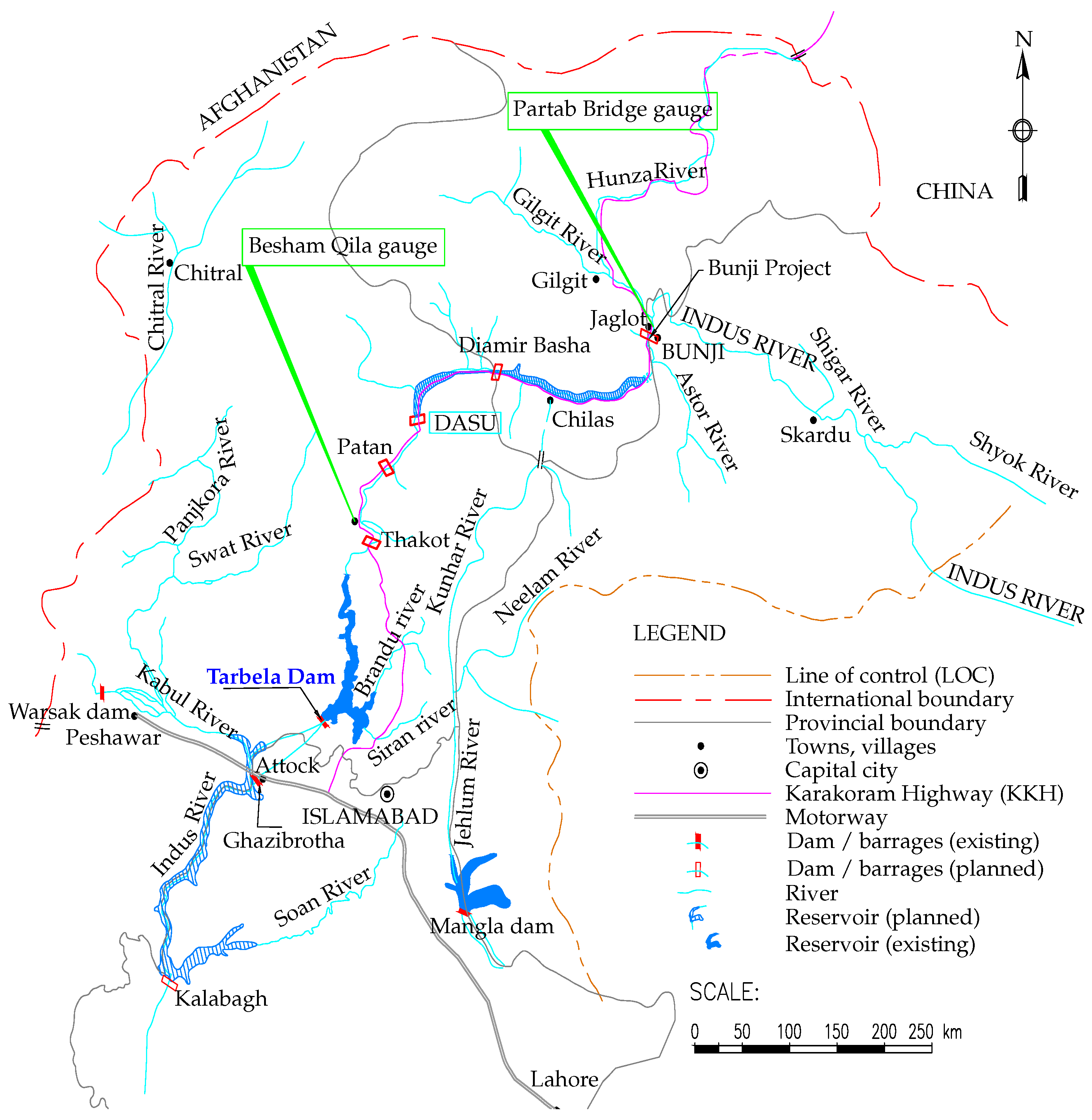
2.1. Study Area
2.2. Data Description
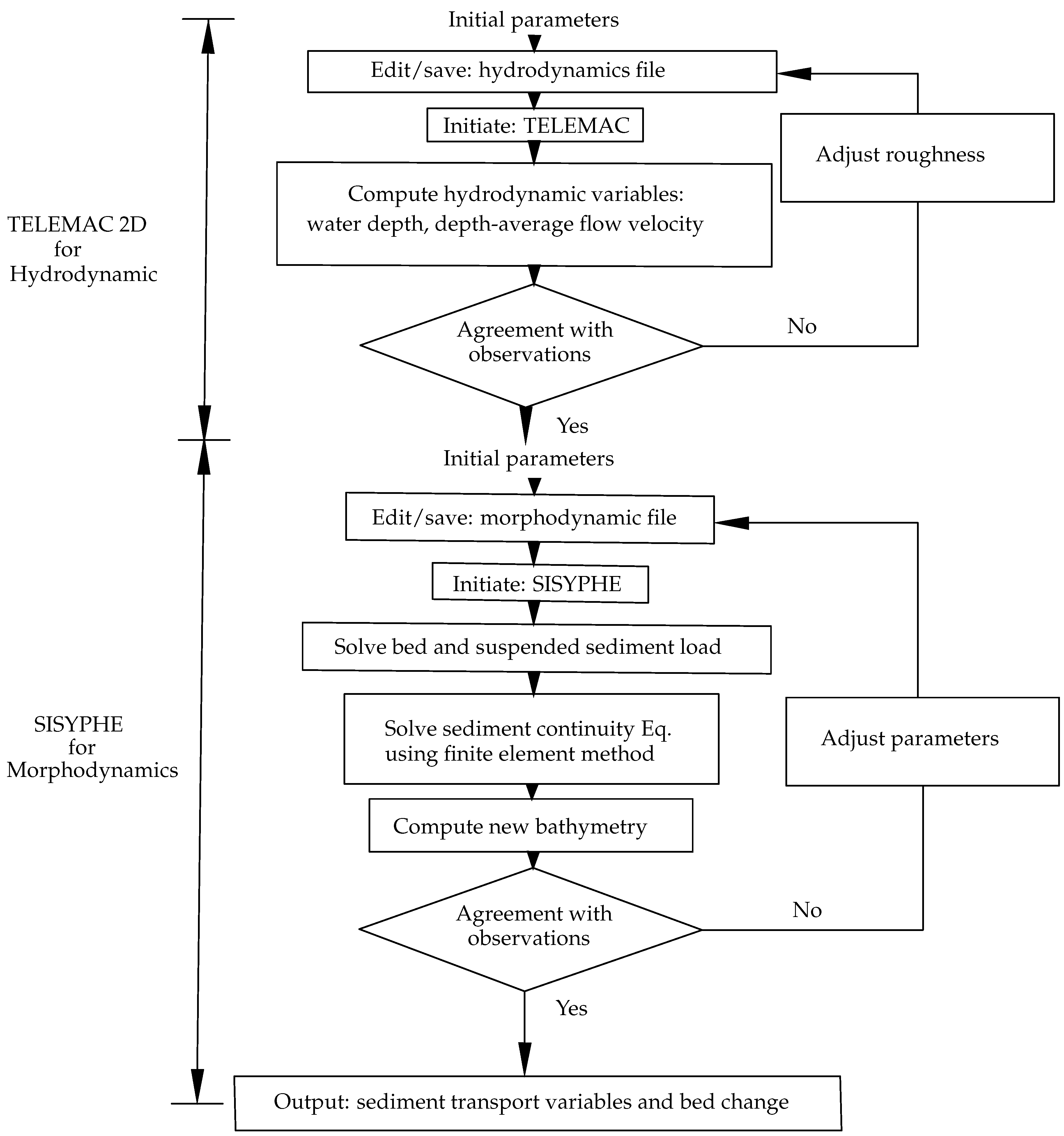
2.3. Model System
2.3.1. TELEMAC-2D for Hydrodynamics
2.3.2. SISYPHE for Morphodynamics
2.4. Model Setup
2.4.1. Grid Mesh
2.4.2. Initial and Boundary Conditions
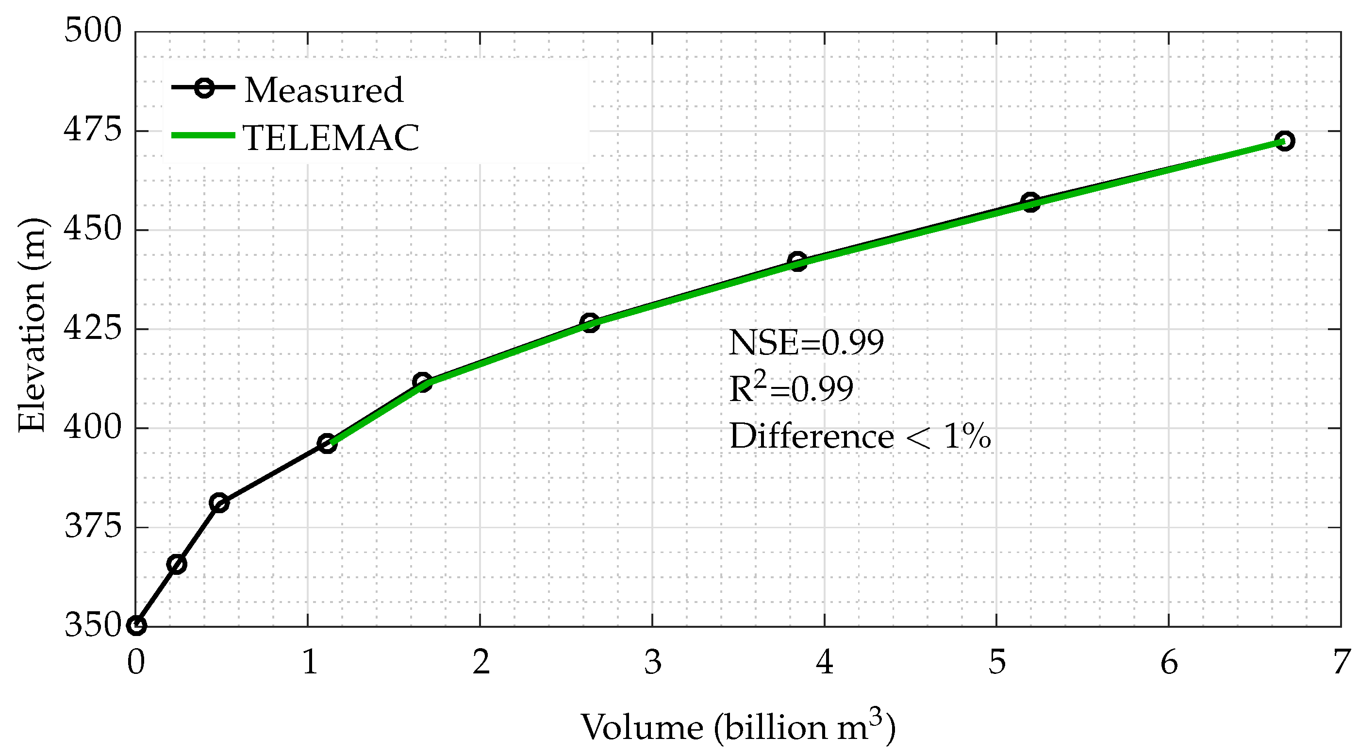
2.5. Model Performance
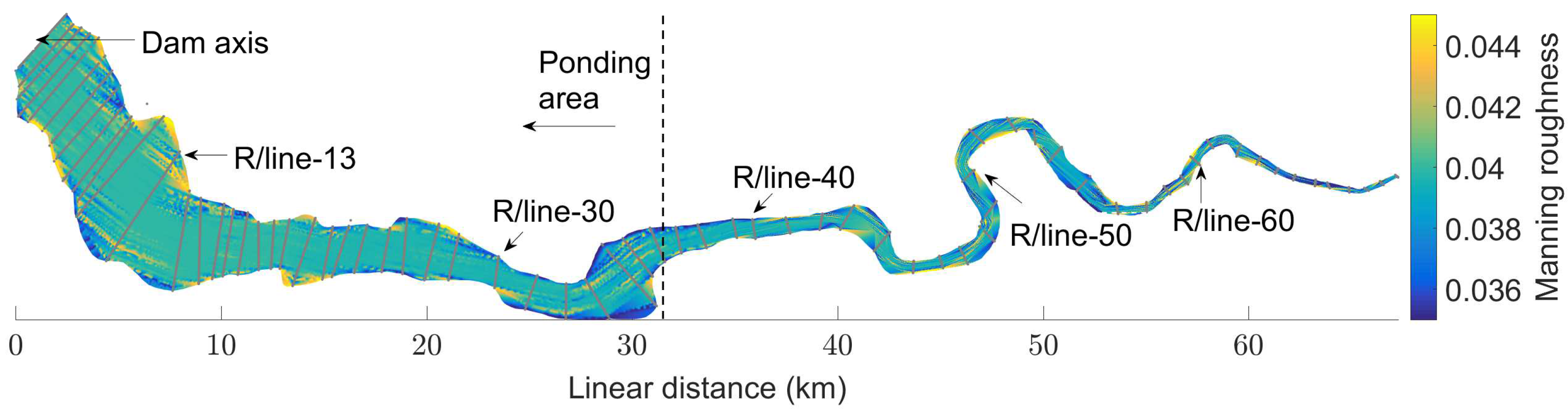
2.6. Model Parameters and Automatic Calibration
- volume of sediments deposited each year after the flood season (between October–November),
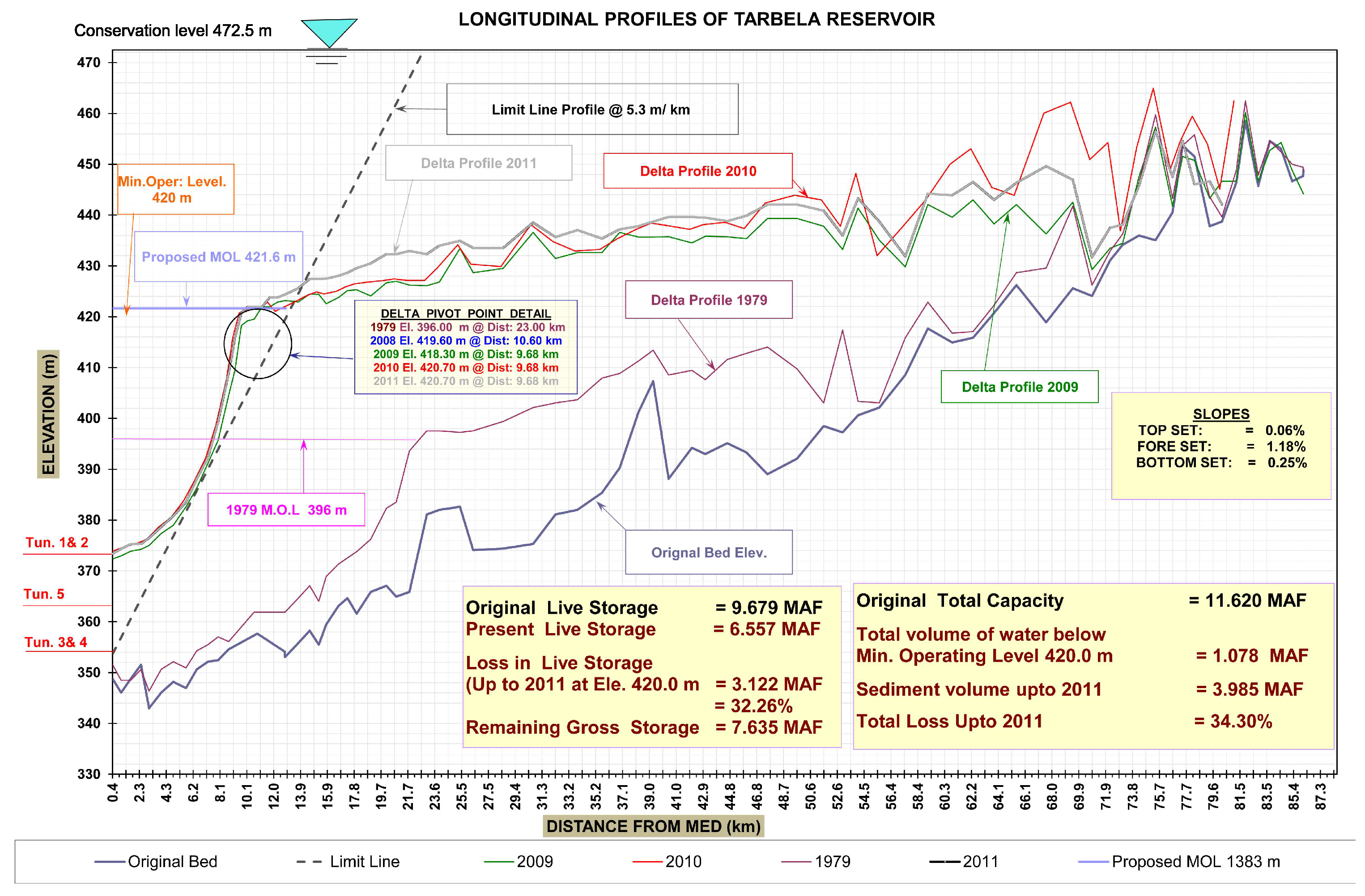
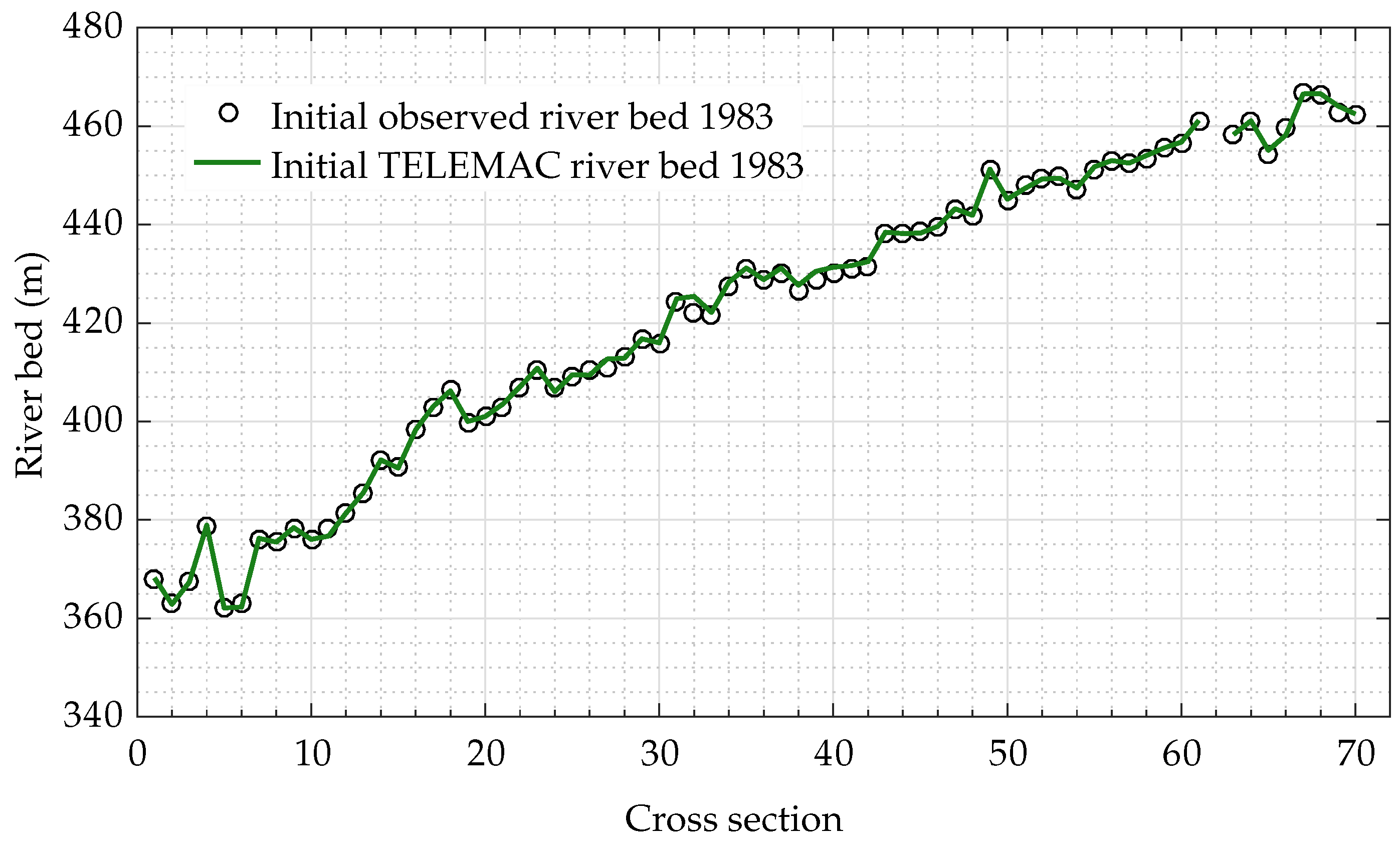
- 72 longitudinal profiles along the reservoir over the period 1983 to the present,
- composition of the sediment deposits in some areas,
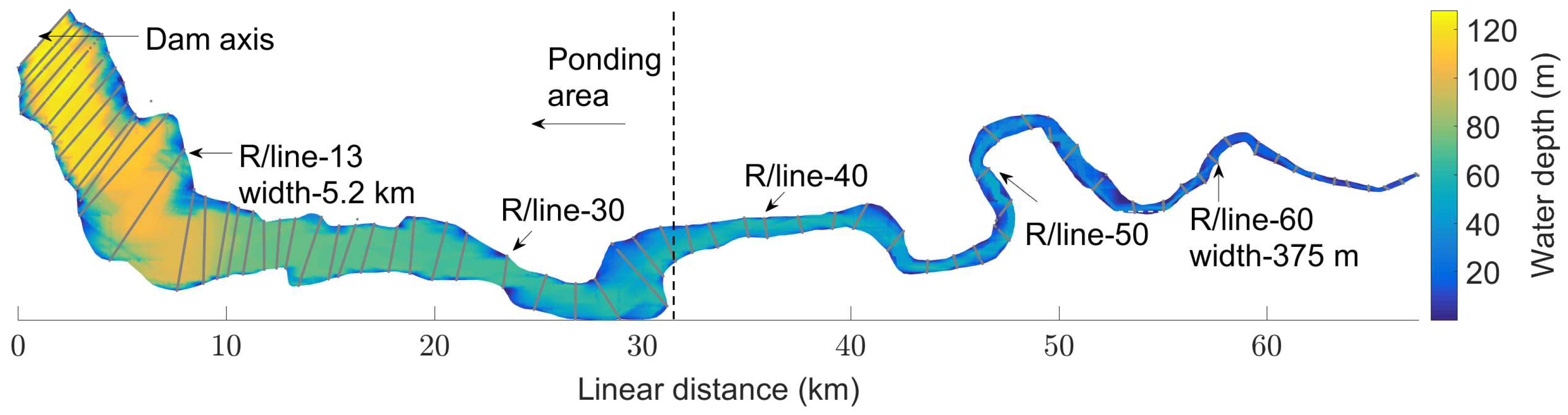
- flow velocities measured with an ADCP at several cross sections,
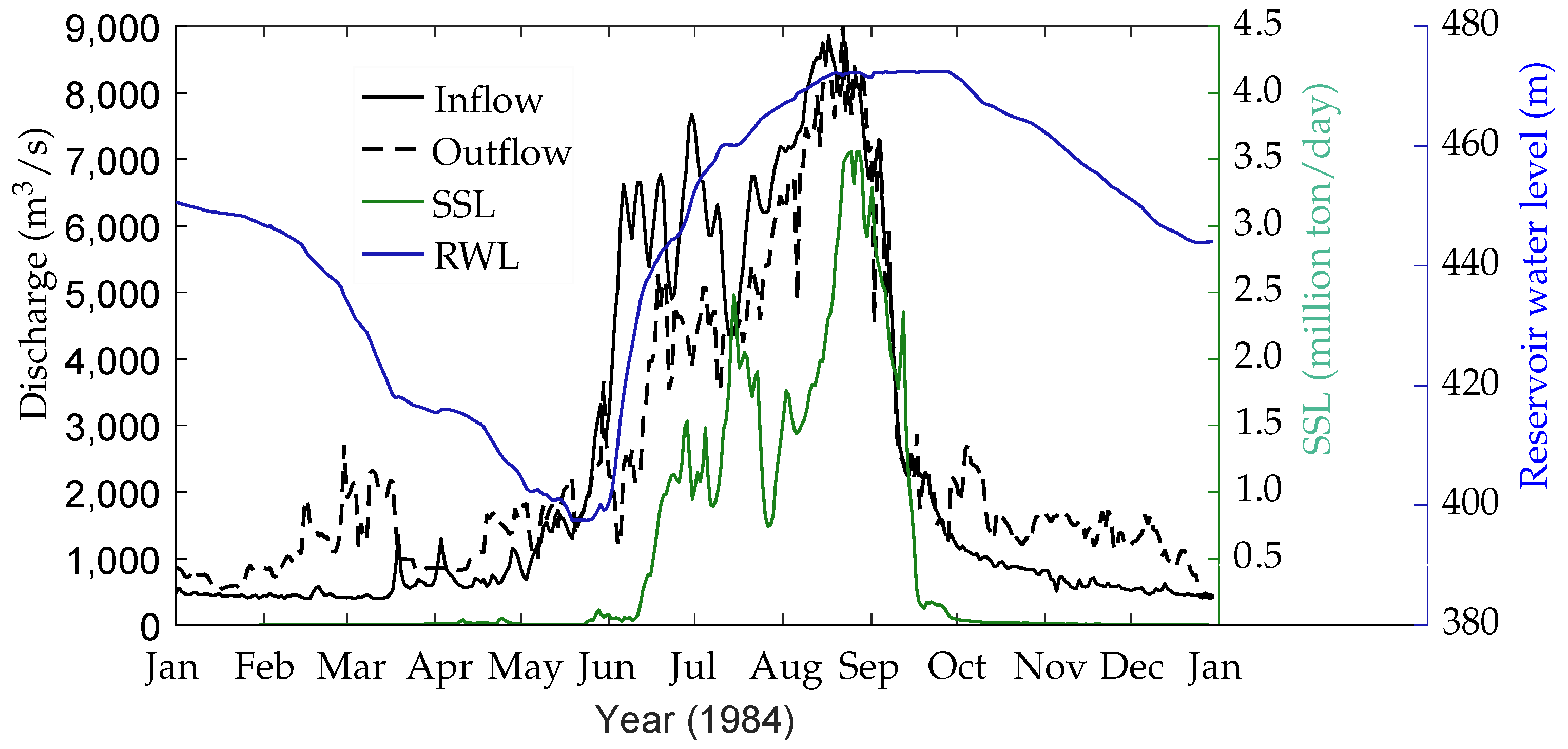
- outflow discharge and sediment concentration.
- linear,
- nearest point,
- natural, and
- cubic
3. Results
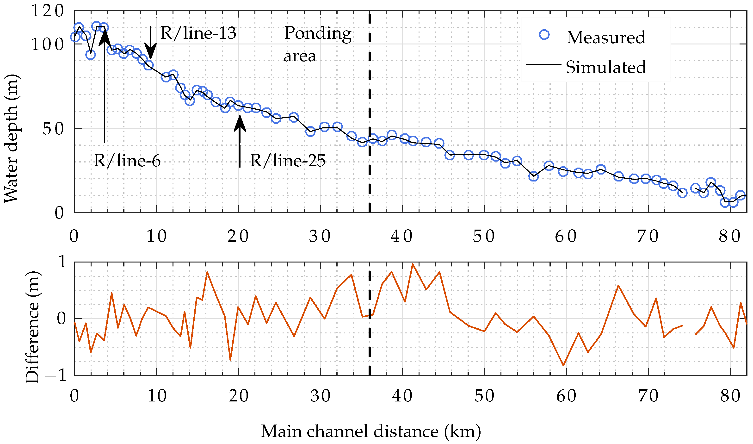
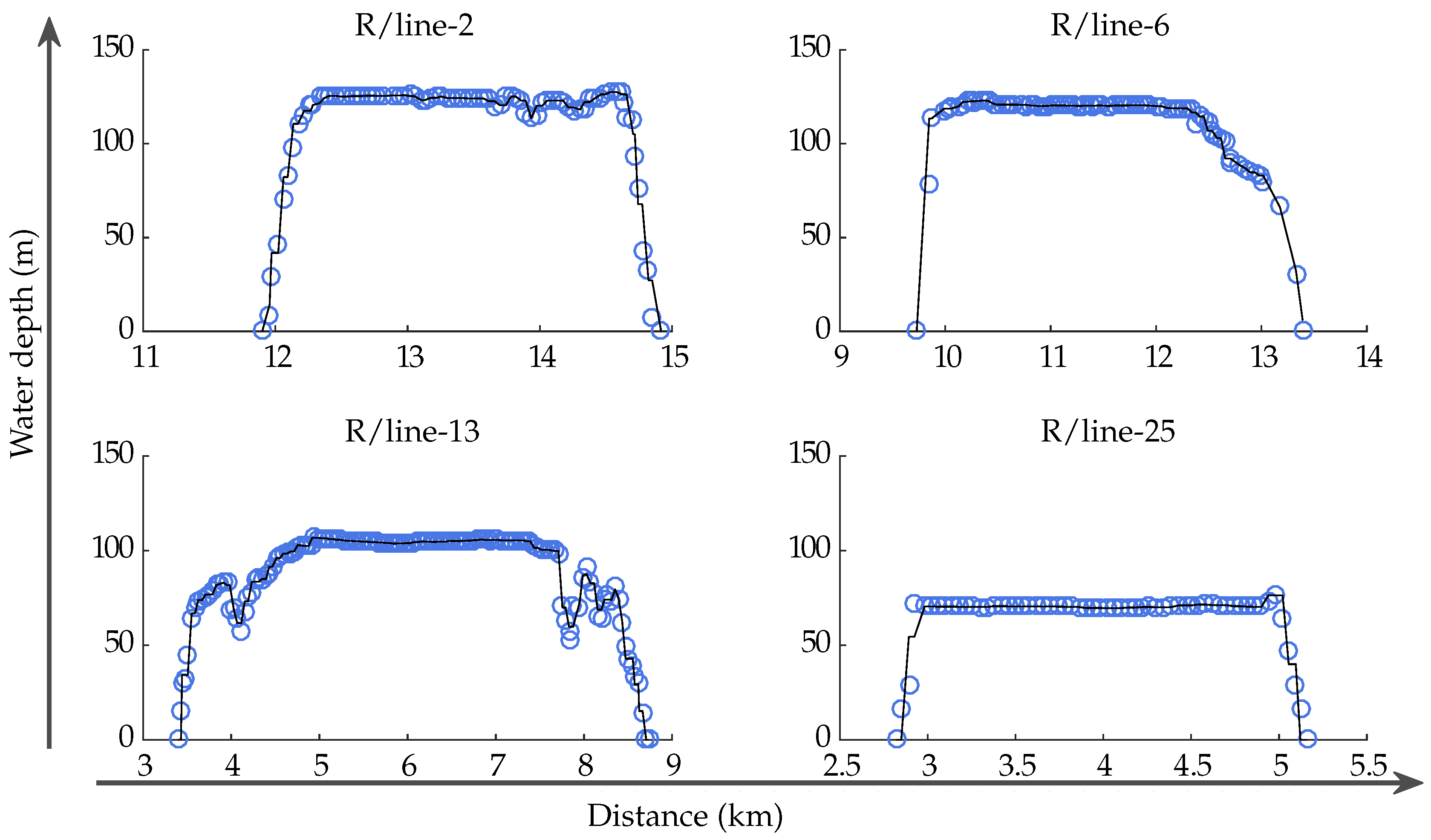
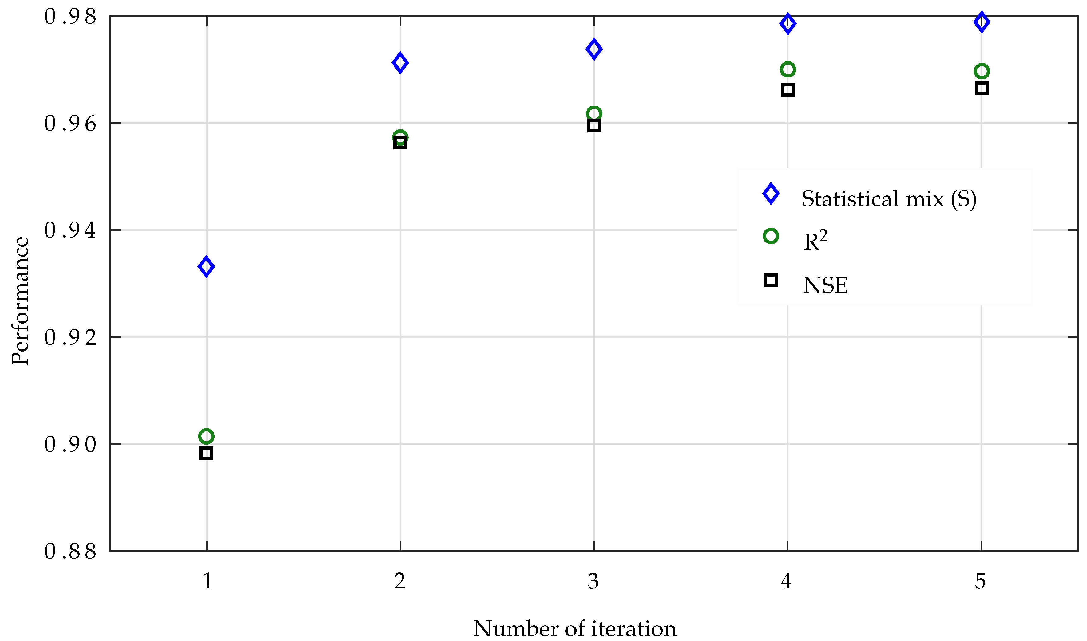
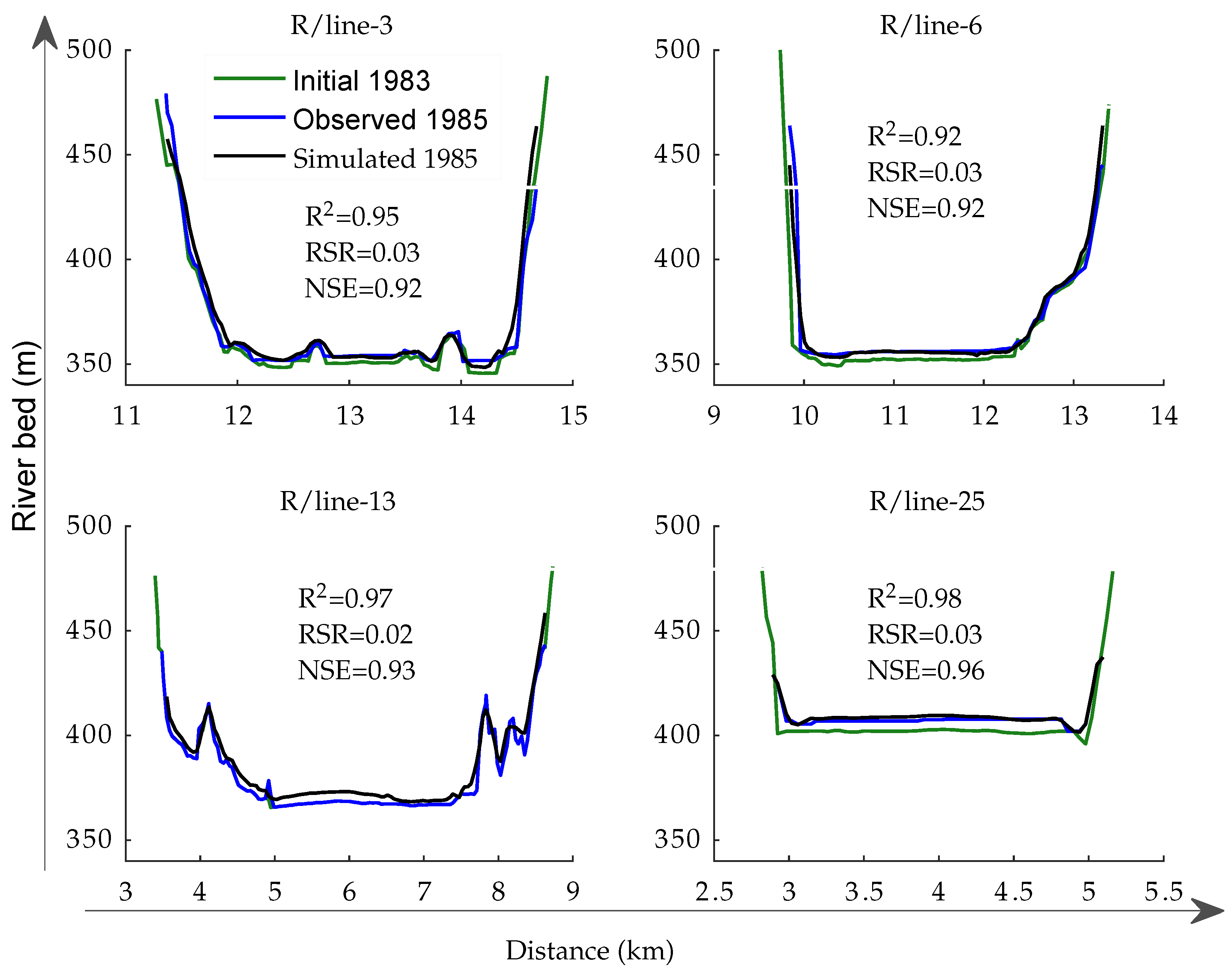
3.1. Model Calibration
- linear,
- nearest point,
- natural, and
- cubic.
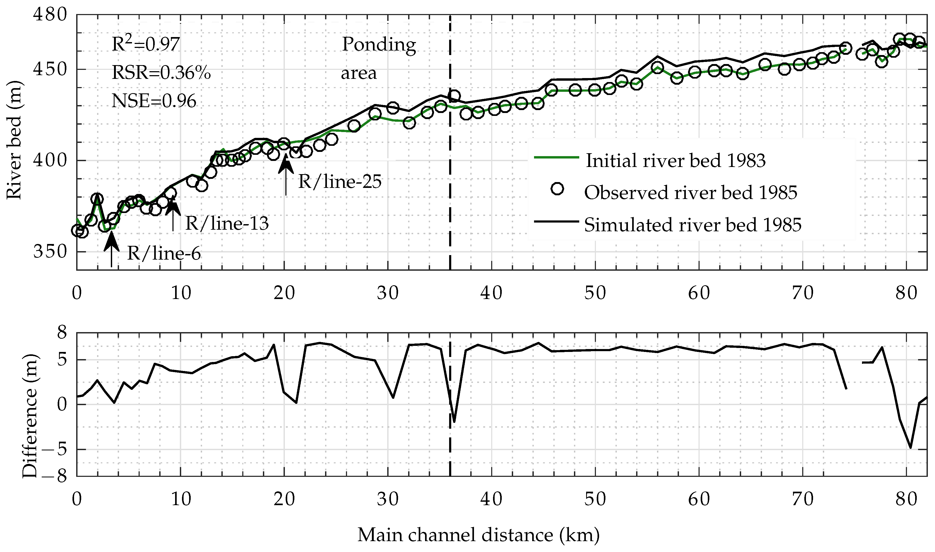
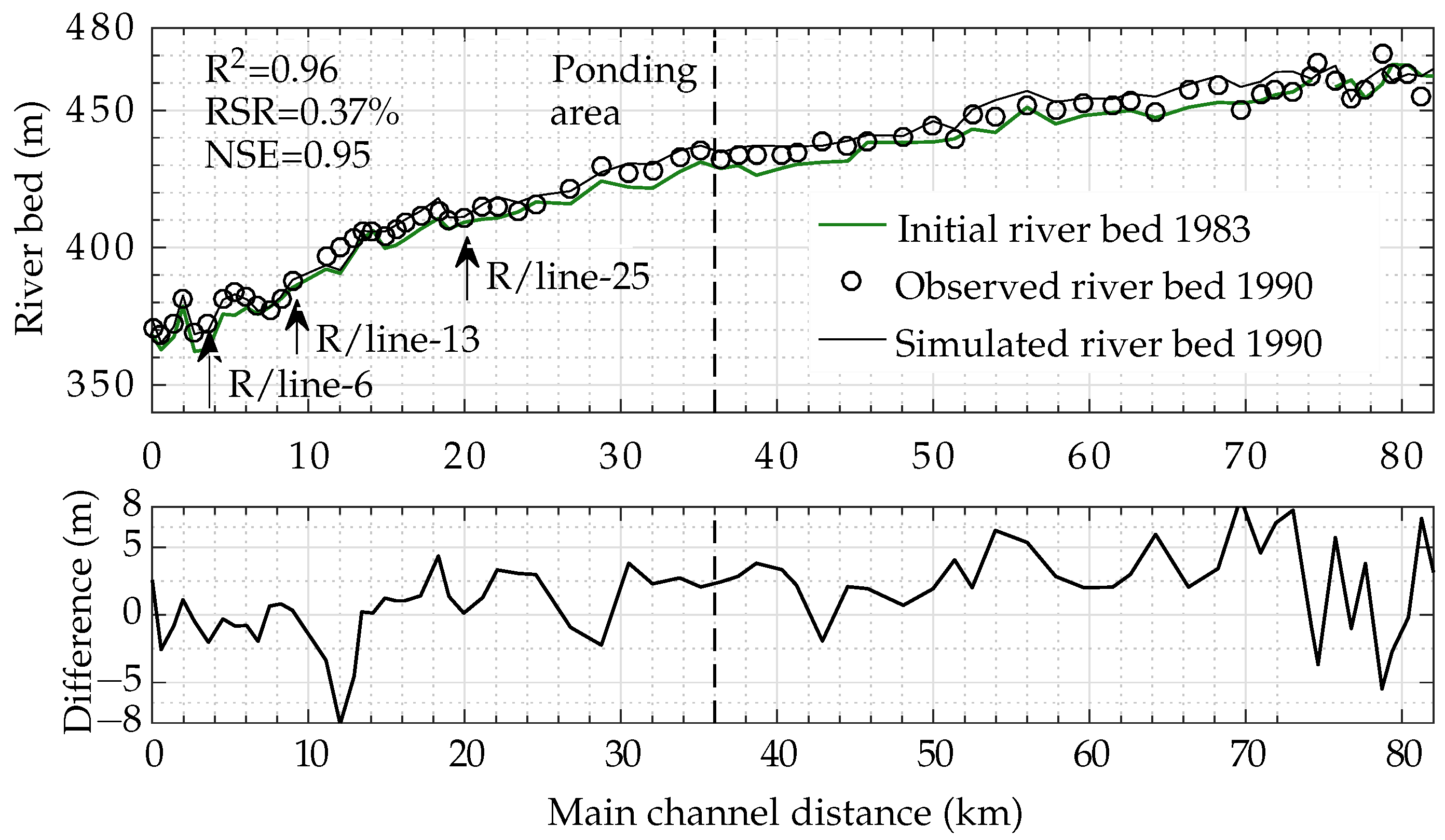
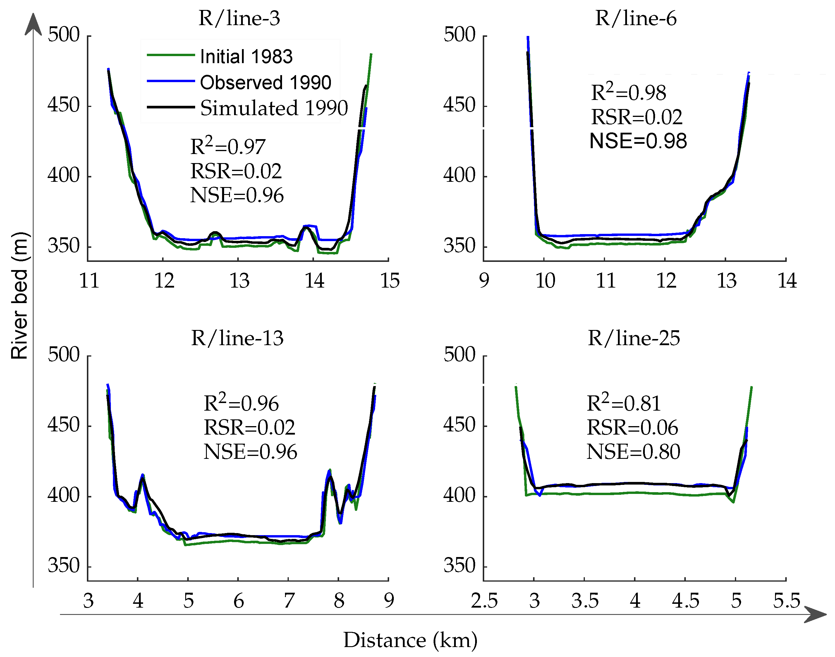
3.2. Model Validation
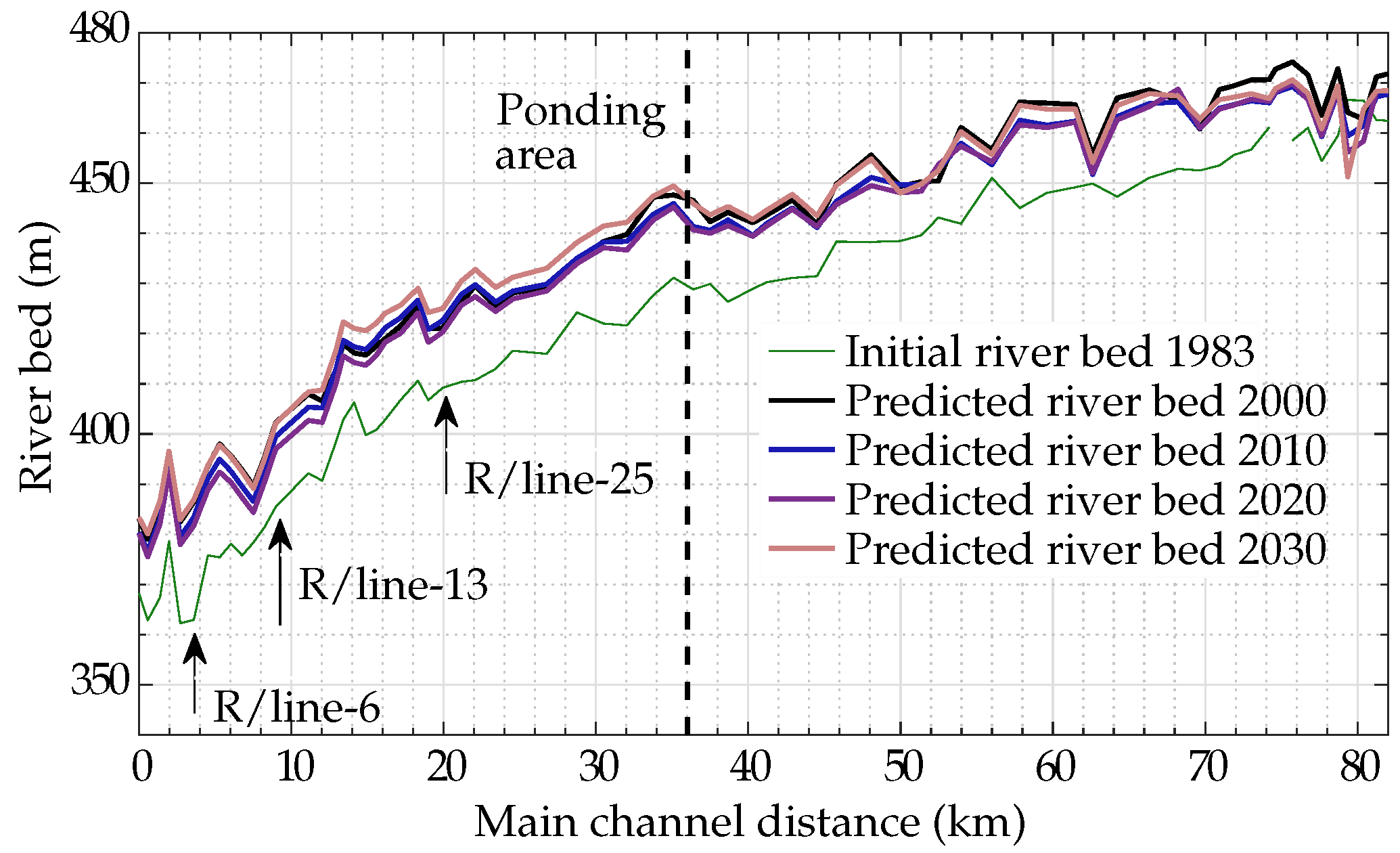
3.3. Model Application
4. Discussion
- inflow of both discharges and SLs,
- particle size distribution of sediments,
- specific weight of sediment deposits,
- geometry of the reservoir, and
- reservoir operation rules [51].
5. Conclusions
- More accurate WA-ANN estimated sediment load boundary conditions which better represent the hysteresis phenomenon and hydrological variations for the Indus River enabled the successive morphodynamic model to accurately predict the bed level changes in the Tarbela dam.
- Automatically calibrating hydrodynamics improved the overall statistical performance and reduced the calculation time for long-term simulations. In addition, specifying the bed roughness for each mesh node using the back propagation error method subsequently enhanced the performance of morphodynamic calculations by providing better hydrodynamic variables and total bed roughness for the calculation of sediment erosion, transport and deposit in the flow area.
- The desynchronization between glacier melt and monsoon rainfall due to warmer climate will also cause a significant decrease in future sediment loads and subsequent delta development. Therefore, past hydro-meteorological data (showing higher sediment loads) cannot be used without modification when making future predictions, particularly for the hydropower projects planned at the Indus River/Basin.
- The presented modelling concept can be used to improve/design sediment management strategies for the existing and planned hydraulic structures in other non-gauged or poorly-gauged rivers.
- Although the effect of the bed roughness on the water depths in large dams is not always dominant, the concept of an automatic hydrodynamic calibration can also be used for other water bodies where roughness has a significant influence on water depths.
- In order to reduce computational time for long-term morphodynamic predictions, coupling of the TELEMAC 2D model with a 1D model/ANN is recommended.
Supplementary Materials
Author Contributions
Funding
Acknowledgments
Conflicts of Interest
Abbreviations
| ADCP | Acoustic Doppler Current Profiler |
| BCM | billion cubic meter |
| sediment concentration in bed load layer | |
| equilibrium near-bed concentration | |
| roughness coefficient | |
| combined friction of both drag forms and skin friction | |
| mean diameter | |
| dimensionless grain diameter | |
| observed water depth | |
| simulated water depth | |
| g | gravitational acceleration |
| h | water depth |
| HEC-RAS | Hydrologic Engineering Center-River Analysis System |
| k | von Karman coefficient |
| km | kilometre |
| bed roughness | |
| roughness height | |
| masl | mean above sea level |
| Mt | million ton |
| MW | megawatt |
| n | Manning roughness |
| NSE | Nash–Sutcliffe Efficiency |
| bed porosity | |
| ppm | part per million |
| and | total sediment transport in x and y direction |
| R2 | coefficient of determination |
| R/line | range lines or cross section |
| RESSASS | Reservoir Survey Analysis and Sedimentation Simulation |
| RSR | observations standard deviation ratio |
| RWL | reservoir water level |
| S | statistical mix |
| SL | sediment load |
| SRC | sediment rating curve |
| SSL | suspended sediment load |
| SSC | suspended sediment concentration |
| SUPG | Streamline-Upwinded Petrov–Galerkin |
| t | time |
| depth-averaged flow velocity components in x and y direction | |
| density | |
| and | depth-averaged turbulent stresses |
| bedload layer thickness | |
| erosion rate | |
| deposition rate | |
| observed parameter | |
| simulated parameter | |
| shear stress due to skin friction | |
| critical shear stress | |
| total bed shear stress | |
| bed form coefficient | |
| calibration coefficient | |
| UIB | Upper Indus Basin |
| settling velocity | |
| WA-ANN | wavelet artificial neural network |
| WAPDA | Water and Power Development Authority |
| yr | year |
| bed elevation | |
| reference elevation | |
| free surface elevation |
References
- Basson, G. Management of siltation in existing and new reservoirs. General Report Q. 89. In Proceedings of the 23rd Congress of the CIGB-ICOLD, Brasilia, Brazil; 2009. Available online: http://scholar.sun.ac.za/handle/10019.1/43104 (accessed on 5 October 2018).
- Annandale, G. Sustainable water supply, climate change and reservoir sedimentation management: Technical and economic viability. In Reservoir Sedimentation; Schleiss, A.J., Cesare, G.D., Franca, M.J., Pfister, M., Eds.; Taylor & Francis Group: London, UK, 2014; ISBN 978-1-138-02675-9. [Google Scholar]
- Schleiss, A.J.; Franca, M.J.; Juez, C.; De Cesare, G. Reservoir sedimentation. J. Hydraul. Res. 2016, 54, 595–614. [Google Scholar] [CrossRef]
- WAPDA. Tarbela Dam Project, Residency Survey and Hydrology Organization; Water and Power Development Authority: Lahore, Pakistan, 2017. [Google Scholar]
- Qiu, J. Stressed Indus River threatens Pakistan’s water supplies. Nature 2016, 534, 600–601. [Google Scholar] [CrossRef] [PubMed]
- Immerzeel, W.W.; Van Beek, L.P.; Bierkens, M.F. Climate change will affect the Asian water towers. Science 2010, 328, 1382–1385. [Google Scholar] [CrossRef] [PubMed]
- Pritchard, H.D. Asia’s glaciers are a regionally important buffer against drought. Nature 2017, 545, 169–174. [Google Scholar] [CrossRef] [PubMed]
- Nourani, V.; Baghanam, A.H.; Adamowski, J.; Kisi, O. Applications of hybrid wavelet–artificial intelligence models in hydrology: A review. J. Hydrol. 2014, 514, 358–377. [Google Scholar] [CrossRef]
- Ateeq-Ur-Rehman, S.; Bui, M.D.; Rutschmann, P. Development of a wavelet-ANN model for estimating suspended sediment load in the upper Indus River. Int. J. River Basin Manag. 2017. [Google Scholar] [CrossRef]
- Juez, C.; Hassan, M.A.; Franca, M.J. The origin of fine sediment determines the observations of suspended sediment fluxes under unsteady flow conditions. Water Resour. Res. 2018, 54. [Google Scholar] [CrossRef]
- Ateeq-Ur-Rehman, S.; Bui, M.D.; Rutschmann, P. Variability and trend detection in the sediment load of the Upper Indus River. Water 2018, 10, 16. [Google Scholar] [CrossRef]
- Lutz, A.F.; Immerzeel, W.W.; Shrestha, A.B.; Bierkens, M.F.P. Consistent increase in High Asia’s runoff due to increasing glacier melt and precipitation. Nat. Clim. Chang. 2014, 4, 587–592. [Google Scholar] [CrossRef]
- Khan, F.; Pilz, J.; Amjad, M.; Wiberg, D.A. Climate variability and its impacts on water resources in the Upper Indus Basin under IPCC climate change scenarios. Int. J. Glob. Warm. 2015, 8, 46–69. [Google Scholar] [CrossRef]
- Lutz, A.F.; Immerzeel, W.; Kraaijenbrink, P.; Shrestha, A.B.; Bierkens, M.F. Climate change impacts on the upper Indus hydrology: Sources, shifts and extremes. PLoS ONE 2016, 11, e0165630. [Google Scholar] [CrossRef] [PubMed]
- Khan, F.; Pilz, J.; Ali, S. Improved hydrological projections and reservoir management in the Upper Indus Basin under the changing climate. Water Environ. J. 2017, 31, 235–244. [Google Scholar] [CrossRef]
- Brune, G.M. Trap efficiency of reservoirs. Trans. Am. Geophys. Union 1953, 34, 407–418. [Google Scholar] [CrossRef]
- Dasu Hydropower Consultants. Detailed Engineering Design Report, Part A; Engineering Design; Water and Power Development Authority: Lahore, Pakistan, 2013. [Google Scholar]
- Dasu Hydropower Project. Dasu Hydropower Project, Feasibility Report; Water and Power Development Authority: Lahore, Pakistan, 2009. [Google Scholar]
- Bunji Consultants Joint Venture. Bunji Hydropower Project, Design Report, Volume 2B Sedimentation; Water and Power Development Authority: Lahore, Pakistan, 2010. [Google Scholar]
- Roca, M. Tarbela Dam in Pakistan. Case study of reservoir sedimentation. In Proccedings of River Flow; Munoz, R.E.M., Ed.; CRC Press: London, UK, 2012; ISBN 978-0-415-62129-8. [Google Scholar]
- Ateeq-Ur-Rehman, S.; Riaz, Z.; Bui, M.D.; Rutschmann, P. Application of a 1-D numerical model for sediment management in Dasu Hydropower Project. In Proccedings of the 14th International Conference on Environmental Science and Technology; Lekkas, D., Ed.; Global CEST: Rohdes, Greece, 2015; ISBN 978-960-7475-52-7. [Google Scholar]
- Rehman, H.U.; Rehman, M.A.; Naeem, U.A.; Hashmi, H.N.; Shakir, A.S. Possible options to slow down the advancement rate of Tarbela delta. Environ. Monit. Assess 2018, 190. [Google Scholar] [CrossRef]
- Malik, Y.I.; Munir, J. Hydraulic design of the low level outlets for Dasu dam, Pakistan. Int. J. Hydropower Dams 2011, 18, 41. [Google Scholar]
- Rüther, N. Computational Fluid Dynamics in Fluvial Sedimentation Engineering. Ph.D. Thesis, Fakultet for Ingeniørvitenskap og Teknologi, Trondheim, Norway, 2006. [Google Scholar]
- Dutta, S.; Sen, D. Sediment distribution and its impacts on Hirakud Reservoir (India) storage capacity. Lakes Reserv. Res. Manag. 2016, 21, 245–263. [Google Scholar] [CrossRef]
- Reisenbüchler, M.; Bui, M.D.; Rutschmann, P. Implimentation of a new layer-subroutine for fractional sediment transport in SISYPHE. In XXIIIrd TELEMAC-MASCARET User Conference; Bourban, S., Ed.; HR Wallingford Ltd.: Howbery Park, Wallingford, UK, 2016. [Google Scholar]
- The International Journal on Hydropower & Dams. First power from Tarbela IV in Pakistan. Int. J. Hydropower Dams 2018, 25, 15. [Google Scholar]
- TAMS Consultants and HR Wallingford. Tarbela Dam Sediment Management Study; Main Report; Water and Power Development Authority: Lahore, Pakistan, 1998. [Google Scholar]
- Anwar, A.A.; Bhatti, M.T. Pakistan’s water apportionment Accord of 1991:25 years and beyond. J. Water Resour. Plann. Manag. 2018, 144. [Google Scholar] [CrossRef]
- Lowe, J.; Fox, I. Sedimentation in Tarbela Reservoir, Commission Internationale des Grandes Barrages. Quatorzieme Congres des Grands Barrages: Rio de Janeiro, 1982. Available online: http://www.icold-cigb.net/homefr.asp (accessed on 5 October 2018).
- Ali, K.F. Construction of Sediment Budgets in Large Scale Drainage Basins: The Case of the Upper Indus River. Ph.D. Thesis, Department of Geography and Planning, University of Saskatchewan, Saskatoon, SK, Canada, 2009. [Google Scholar]
- Mehta, A.J.; Lee, S.C. Problems in linking the threshold condition for the transport of cohesionless and cohesive sediment grain. J. Coast. Res. 1994, 10, 170–177. [Google Scholar]
- Klassen, I. Three-Dimensional Numerical Modeling of Cohesive Sediment Flocculation Processes in Turbulent Flows. Ph.D. Thesis, Bauingenieur-, Geo- und Umweltwissenschaften, Karlsruher Instituts für Technologie (KIT), Baden-Württemberg, Germany, 2017. [Google Scholar]
- Ali, K.F.; De Boer, D.H. Spatial patterns and variation of suspended sediment yield in the Upper Indus River Basin, northern Pakistan. J. Hydrol. 2007, 334, 368–387. [Google Scholar] [CrossRef]
- EDF-R&D. TELEMAC v7.0 User Manual; Open TELEMAC-MASCARET: Chatou, France, 2014. [Google Scholar]
- EDF-R&D. Sisyphe v7.2 User’s Mannual; Open TELEMAC-MASCARET: Chatou, France, 2017. [Google Scholar]
- Roelvink, J.A. Coastal morphodynamic evolution techniques. Coast. Eng. 2006, 53, 277–287. [Google Scholar] [CrossRef]
- Duc, B.M.; Bernhart, H.H.; Kleemeier, H. Morphological numerical simulation of flood situations in the Danube River. Int. J. River Basin Manag. 2005, 3, 283–293. [Google Scholar] [CrossRef]
- Juez, C.; Murillo, J.; Garcia-Navarro, P. A 2D weakly-coupled and efficient numerical model for transient shallow flow and movable bed. Adv. Water Resour. 2014, 71, 93–109. [Google Scholar] [CrossRef]
- Reisenbüchler, M.; Bui, M.D.; Skublics, D.; Rutschmann, P. An integrated approach for investigating the correlation between floods and river morphology: A case study of the Saalach River, Germany. Sci. Total Environ. 2019, 647, 814–826. [Google Scholar] [CrossRef] [PubMed]
- Nash, J.E.; Sutcliffe, J.V. River flow forecasting through conceptual models part I—A discussion of principles. J. Hydrol. 1970, 10, 282–290. [Google Scholar] [CrossRef]
- Moriasi, D.N.; Arnold, J.G.; Van Liew, M.W.; Bingner, R.L.; Harmel, R.D.; Veith, T.L. Model evaluation guidelines for systematic quantification of accuracy in watershed simulations. Trans. Asabe 2007, 50, 885–900. [Google Scholar] [CrossRef]
- Rijn, L.C.V. Sediment transport, part II: Suspended load transport. J. Hydraul. Eng. 1984, 110, 1613–1641. [Google Scholar] [CrossRef]
- Van Rijn, L.C. Principles of Sediment Transport in Rivers, Estuaries And Coastal Seas; Aqua publications Amsterdam: Amsterdam, The Netherlands, 1993; ISBN 9080035629. [Google Scholar]
- HR Wallingford. Sedimentation Study, Dasu Hydropower Project; Report EX 6801 R1; Dasu Hydropower Consultants; Water and Power Development Authority: Lahore, Pakistan, 2012. [Google Scholar]
- Talmon, A.M.; Struiksma, N.S.; van Mierlo, M.C.L.M. Laboratory measurements of the direction of sediment transport on transverse alluvial-bed slopes. J. Hydraul. Res. 1995, 33, 495–517. [Google Scholar] [CrossRef]
- Bolch, T. Hydrology: Asian glaciers are a reliable water source. Nature 2017, 545, 161–162. [Google Scholar] [CrossRef] [PubMed] [Green Version]
- Hasson, S. Future water availability from Hindukush-Karakoram-Himalaya Upper Indus Basin under conflicting climate change scenarios. Climate 2016, 4, 40. [Google Scholar] [CrossRef]
- Rumelhart David, E.; McClelland, J.L. Parallel Distributed Processing, v. 1, Foundations Explorations in the Microstructure of Cognition Foundations; MIT Press: Cambridge, UK, 1986. [Google Scholar]
- Jain, S.K. Development of integrated sediment rating curves using ANNs. J. Hydraul. Eng. 2001, 127, 30–37. [Google Scholar] [CrossRef]
- USBR. Design of Small Dams; Water Resources Technical Publication: New York, NY, USA, 1987; 860p. [Google Scholar]
- Salas, J.D.; Shin, H.S. Uncertainty analysis of reservoir sedimentation. J. Hydraul. Eng. 1999, 125, 339–350. [Google Scholar] [CrossRef]
- Holeman, J.N. The sediment yield of major rivers of the world. Water Resour. Res. 1968, 4, 737–747. [Google Scholar] [CrossRef]
- Peshawar University. The Sediment Load and Measurements for Their Control in Rivers of West Pakistan; Department of Water Resources, Peshawar University: Peshawar, Pakistan, 1970. [Google Scholar]
- Pickup, G. Adjustment of stream-channel shape to hydrologic regime. J. Hydrol. 1976, 30, 365–373. [Google Scholar] [CrossRef]
- Kumar, R.; Kumar, R.; Singh, S.; Singh, A.; Bhardwaj, A.; Kumari, A.; Randhawa, S.S.; Saha, A. Dynamics of suspended sediment load with respect to summer discharge and temperatures in Shaune Garang glacierized catchment, Western Himalaya. Acta Geophys. 2018, 66, 1–12. [Google Scholar] [CrossRef]


| Process | Duration | R2 | RSR | NSE |
|---|---|---|---|---|
| Calibration | 1984–1985 | 0.842 | 0.019 | 0.837 |
| Validation | 1986–1990 | 0.888 | 0.019 | 0.871 |
| Sand | ||||||
|---|---|---|---|---|---|---|
| Grain size (mm) | 1.0 | 0.5 | 0.25 | 0.125 | 0.0625 | Pan |
| Fraction (%) | 100 | 99.87 | 96.98 | 85.85 | 71.98 | 71.97 |
| Silt | ||||||
| Grain size (mm) | 0.0442 | 0.0312 | 0.0221 | 0.0156 | 0.011 | 0.0078 |
| Fraction (%) | 64.51 | 57.12 | 49.59 | 41.07 | 32.70 | 25.29 |
| Clay | ||||||
| Grain size (mm) | 0.0055 | 0.0039 | ||||
| Fraction (%) | 17.43 | 10.32 | ||||
| Months | Average SSL (Mt) | Average inflow (BCM) | Average outflow (BCM) |
|---|---|---|---|
| Jan–Apr | 0.98 | 5.67 | 11.85 |
| May–Sep | 157.9 | 65.54 | 55.18 |
| Oct–Dec | 1.11 | 5.50 | 11.25 |
| Parameter | Value/methods |
|---|---|
| Hydrodynamics | |
| Numerical scheme | Centred semi implicit scheme plus SUPG |
| Solver for hydrodynamic propagation step | Generalized minimum residual method |
| Equations | Saint-Venant finite element |
| Hydrodynamic calibration factor (K) | 1.0 |
| Manning roughness (n) | 0.035–0.045 |
| Mean Manning roughness (n) | 0.0395 |
| TELEMAC and SISYPHE model coupling | Internal |
| Morphodynamics | |
| Bed porosity () | 0.375 |
| Fluids viscosity () | |
| Suspended sediment transport formula | [43] |
| Calibration coefficient () | 3 |
| von Karman coefficient (k) | 0.40 |
| Shields parameter | 0.047 |
| Friction angle of sediment () | 32 |
| Minimum depth required for sediment transport | 1 cm |
| Formula for deviation | [46] |
| Parameter for deviation () [46] | 0.85 |
| Stream wise slope effect () | 1.3 |
| Solver for suspension | Conjugate gradient |
| Critical evolution ratio | 0.5 |
| Numerical treatment of the advection term | Edge-based N-scheme |
© 2018 by the authors. Licensee MDPI, Basel, Switzerland. This article is an open access article distributed under the terms and conditions of the Creative Commons Attribution (CC BY) license (http://creativecommons.org/licenses/by/4.0/).
Share and Cite
Ateeq-Ur-Rehman, S.; Bui, M.D.; Hasson, S.U.; Rutschmann, P. An Innovative Approach to Minimizing Uncertainty in Sediment Load Boundary Conditions for Modelling Sedimentation in Reservoirs. Water 2018, 10, 1411. https://doi.org/10.3390/w10101411
Ateeq-Ur-Rehman S, Bui MD, Hasson SU, Rutschmann P. An Innovative Approach to Minimizing Uncertainty in Sediment Load Boundary Conditions for Modelling Sedimentation in Reservoirs. Water. 2018; 10(10):1411. https://doi.org/10.3390/w10101411
Chicago/Turabian StyleAteeq-Ur-Rehman, Sardar, Minh Duc Bui, Shabeh Ul Hasson, and Peter Rutschmann. 2018. "An Innovative Approach to Minimizing Uncertainty in Sediment Load Boundary Conditions for Modelling Sedimentation in Reservoirs" Water 10, no. 10: 1411. https://doi.org/10.3390/w10101411