Enumerating the Effects of Climate Change on Water Resources Using GCM Scenarios at the Xin’anjiang Watershed, China

Abstract

The present study developed a novel approach to study the climate change impact on the water resources and generation of hydropower optimally using forecasted stream flows for the Xin’anjiang water shed in China. Future flows were projected using six large-scale Global circulation models (GCMs) with RCP4.5 and RCP8.5 scenarios. A newly developed mathematical modeling using particle swarm optimization was incorporated to work out the projected optimal electricity generation from the Xin’anjiang hydropower station. The results reveal that watershed will be warmer by the end of the 21st century with a maximum increase of up to 4.9 °C for mean maximum, and 4.8 °C for mean minimum temperature. Six GCMs under Representative Concentration pathways (RCPs) showed that future precipitation is complex to predict with certainty and significant differences were observed among the different GCMs. The overall mean monthly and seasonal precipitation increase for most scenarios with the maximum increase during the 2020s and 2080s, whereas 2050s exhibited the lesser increase. Resultantly, there would be an increase in the stream flows during these periods, which was used for electricity production up to 31.41 × 10⁸ kW·h.

1. Introduction

China is the world’s most populated country and a core emitter of greenhouse gases. Therefore, the major thrust of their current research is on climate change but comparatively little has been published so far. Global air temperature trends show a rise of 0.85 °C between 1880 and 2012 with a higher contribution during the last 30 years [1]. China is no exception to this phenomenon, and water resources of China are highly sensitive to climate change [2,3,4,5]. Research studies show that particularly the northern parts of China are becoming warmer more rapidly than the southern parts [6,7], and it is predicted that the average temperature in China will increase by +3.9 to 5.6 °C by the end of 2100 under B2 and A2 scenarios, respectively [8].

Several regional and local scale studies have been conducted to study the climate change impacts on Chinese water resources and on an estimation of precipitation trends in different parts of China. Ding et al. reported non-significant annual averaged precipitation trends in the country, while interdecadal trends and variability have been found on a regional basis [9]. Meanwhile [6,10] have found a decreasing trend in the mean annual precipitation during 1961–2001 in the northeastern, northern and central regions of China. Piao et al. [6] found North China and Northeast China are receiving less and less precipitation in summer and autumn compared to the wetter region of southern China, which is experiencing more rainfall during both summer and winter. Feng et al. [11] found a significant increase in both extreme precipitation and mean annual precipitation intensity over south-eastern China. A significant increasing trend has been found in south-western and south-eastern China [12]. Studies have also reported an adjustment in the precipitation trends in eastern China since the 1970s [13,14], with southern China and the Yangtze River basin suffering the most by precipitation and severe flooding, while northeastern and northern China experienced severe droughts [9,15]. On the local scale, Wang et al. [16] used precipitation data from 1961–2008 of the Jinshajiang River basin and found insignificant increases in trends. Li and Yan [17] observed decreasing trends in the annual precipitation in the Mianyang Basin of Sichuan Province, China. Xu et al. [18] have observed an increase in precipitation amount during 1960–2007 in the Tarim River basin. Although many large-scale watershed studies have been carried out in different regions of China [19,20], not much work has been done to determine the climate change effects on water resources in medium-scale watersheds particularly in the current study region, which could be very important for water supply and power production.

General Circulation Models (GCMs) have been found to be promising tools for the prediction of future climatic scenarios [21] and future assessment not only for the surface hydrology but also for water allocation and modeling of the groundwater resources [22,23,24,25,26,27]. To evaluate regional changes in daily rainfall and temperature, global climate model (GCM) output needs to be downscaled to a local appropriate scale. Many approaches to attain this can be generally classified as dynamical, and statistical downscaling techniques [28]. In any case, some adjustments need to be made before the use of any downscaled data to account for the GCM biases [29]. We emphasize here a common method of bias correction, namely quantile mapping technique, which has been used extensively for downscaling precipitation and temperature [30,31,32] around the globe. The quantile mapping method has the advantage of accounting for GCM biases in all statistical moments; however, as with all other statistical downscaling methods, it is expected that biases will be constant in the future projections. Quantile mapping has some drawbacks, so the calibration period for the bias correction should be at least 10 years so that the internal inconsistency is not a leading source of bias between the climate model and observations [33]. Despite its drawbacks, this technique is extensively used and commonly effective in removing biases [34,35,36,37,38].

Coupling of climate models with hydrological models such as the Soil and Water Assessment Tool (SWAT, developed by the Agricultural Research Service and the US Department of Agriculture, USA) is widely used for the simulation of stream flows, sediment yields and loss of nutrients in watersheds [39], which is well validated all over the world including America [40], Europe [41], Australia [42], Africa [43], and Asia [44,45,46]. As water resources have become more important, their optimal use and allocation also become very important yet complex. During 1970–1980, some algorithms were developed for the solution of problems through optimization. For instance, programming techniques such as linear, nonlinear and dynamic have been applied to find the solutions to the problems of reservoir operation [47,48,49]. Several studies have used these techniques for the solution of multidimensional problems [50,51,52]. Particle swarm optimization (PSO) is another popular optimization technique developed by [53]. This technique performed significantly robustly for the solution of multi-stage continuous optimal hydropower generation and performed better than other techniques to find the optimal solution of hydropower optimization [46,54,55,56]. Contrary to the previous studies [57,58,59,60,61,62], this paper is written with an overall goal to project future stream flows hydrologically, and to figure out the projected hydropower generation based on these future streamflows with the application of a newly developed numerical model for Xin’anjiang hydropower station.

2. Location of the Study Area

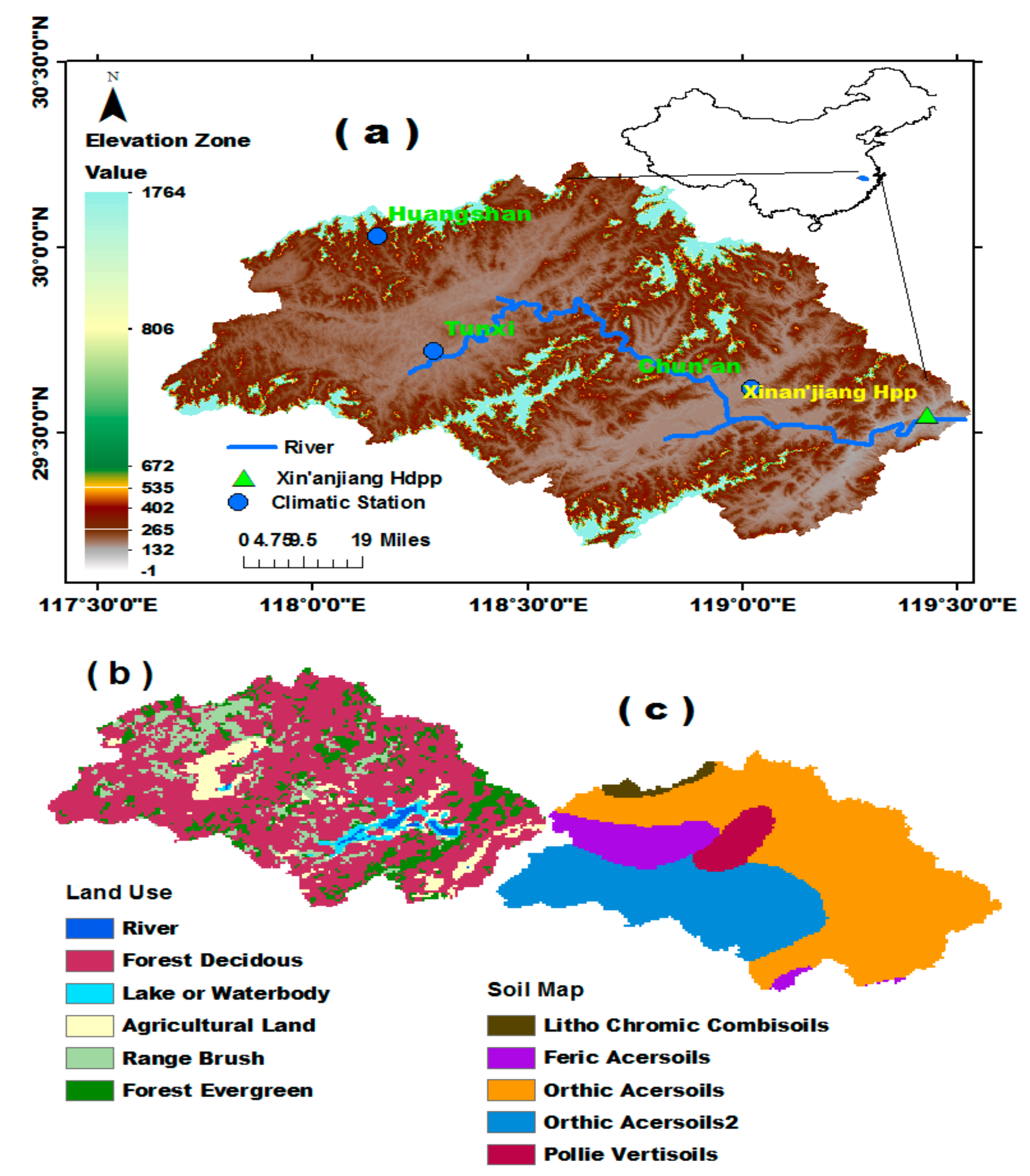
Xin’anjiang watershed is located between 117°38′15″–119°31′56″ longitude and 29°11′9.9″–30°13′49″ latitude, as shown in Figure 1a. The watershed has an area of about 11,675.710 km². The average annual rainfall is more than 500 mm. There is a famous hydropower station in the study area named as Xin’anjiang hydropower station, which is situated at the Qiantang River tributary named as Xin’an River, with a total capacity of 845,000 kW and annual estimated output of 1.86 billion kW·h (18.6 × 10⁸ kW·h).The location of the hydropower station is 29°28′38″ Latitude and 119°13′31″ Longitude in the Xin’anjiang watershed where a well-known China’s oldest Xin’anjiang Dam (466.5 m long and 105 m high) is located. This dam carries a huge reservoir capacity of about 22 billion m³ and flood discharging capability of 14,000 m³/s. The dam reservoir links Mount Huangshan of Anhui Province with Hangzhou, which is the capital of Zhejiang province. The average discharge of the river upstream of the Hangzhou City is 1043 m³/s. The flow in the river is higher during March to July and lower in the remaining months.

Mainly the water supply of Hangzhou Region depends on the Qiantang River. Water is distracted directly from this river through various intakes and no severe water shortages have been observed in the recent years, yet flooding remains an important issue. The region is currently going rapid economic development and population growth and, these developments, in combination with climate change effects, expecting to cause future changes in the water supplies and demands.

Furthermore, About 1708 km² area is considered irrigated land (out of which 1571 km² irrigated by the Xin’anjiang reservior) in the Xin’anjiang watershed with major crops including rice, wheat, soybean, potato, corn and some other high value crops The changes in the water resources not only affects the domestic water availability, but also can affect the command area under irrigation and hydropower generation.Moreover, changes in the future flows may harmful for the dam structure and can cause severe damages.

3. Data Collection

Daily metrological data of precipitation, maximum and minimum temperature, wind speed and solar radiation for the period of 1979–2010 was obtained from the China Metrological Department (http://data.cma.cn/). Six GCMs (CCSM4, HadGEM2-ES, MPI-ESM-MR, MPI-ESM-LR, ACCESS1.0 and MIROC-ESM) of CMIP5 (Coupled Model Intercomparsion Project Phase 5, https://cmip.llnl.gov/index.html?submenuheader=0) were selected for future hydrological projections under very high (RCP8.5) and medium stabilization scenarios (RCP4.5). The GCMs models are divided into different scenarios as given in

Table 1. GCMs models with RCPs.

Model/RCP *	Institutes and Grid Resolution	RCP4.5	RCP8.5
CCSM4	(National center for Atmospheric Research USA with 0.9424° × 1.25° grid resolution)	Designated as C 4.5	Designated as C 8.5
HadGEM2-ES	(Met office Hadley Centre UK with 1.875° × 1.25° grid resolution)	Designated as H 4.5	Designated as H 8.5
MPI-ESM-LR	(Max Plank Institute for Metrology, Hamburg, Germany with 1.8653° × 1.875° grid resolution)	Designated as LR 4.5	Designated as LR 8.5
MPI-ESM-MR	Max Plank Institute for Metrology, Hamburg, Germany with 1.865 × 1.875° grid resolution	Designated as MR 4.5	Designated as MR 8.5
ACCESS 1.0	(Commonwealth Scientific and Industrial Research Organization (CSIRO) and Bureau of Metrology, Australia with 1.875° × 1.25° grid resolution)	Designated as A 4.5	Designated as A 8.5
MIROC-ESM	(University of Tokyo, NIES and JAMSTEC with 2.7906° × 2.8125° grid resolution)	Designated as MI 4.5	Designated as MI 8.5

* Global Circulation models (GCM); Representative Concentration pathways (RCP); The Community Climate System Model version 4 (CCSM4); The Hadley Center Global Environment Model Version 2 (HadGEM2-ES); Max Plank Institute, Earth System Model with Low Resolution (MPI-ESM-LR); Max Plank Institute, Earth System Model with Medium Resolution (MPI-ESM-MR); Australian Community Climate and Earth Simulator Version 1 (ACCESS1.0); Model for interdisciplinary Research on Climate (MIROC-ESM).

. The future climatic parameters such as precipitation, maximum and minimum temperature, winnd speed and solar radition were downscaled for these six GCMs to a finer scale. The selection of these GCMs is based on the previous studies conducted in the current region [46,63,64,65]. The analysis is based on the metrological data from 1979 to 2010. The downscaled data of six GCMs for three future periods of 2010–2039, 2040–2069 and 2070–2099, have been termed as the 2020s (near future), 2050s (far future) and 2080s (very far future), respectively. The hydrological data series (Streamflows) of the watershed are required for the calibration and validation of the model. The streamflows data were collected from the Hydrology Bureau of Zhejiang Province. Streamflows data from 1979–1993 were used for the calibration, while the data from 1994–2005 were used for the validation of the hydrological model.

4. Materials and Methods

4.1. Functionality of SWAT

The SWAT hydrological model is a basin-scale continuous model that operates on a daily time step basis [66]. The model was developed by the Agricultural Research Service and the US Department of Agriculture to predict the effects of land management practices on sediment, water and agricultural chemicals. For modeling of different processes, the watershed is divided into several sub-basins, which are further divided into hydrological response units (HRU) according to land use, soil properties and slope of the area. SWAT simulates watershed hydrology together with sediment, chemical pesticides and nutrients from every HRU along with the water flows in the irrigation channels [67].

Modified rational numbers are used to calculate the peak stream flows in the SWAT model [68]. A kinematic storage routing model is used to determine the sub-surface flows up to 2 m depth in each soil layer [69] and a shallow aquifer storage area is created to gauge the groundwater flow contribution [70]. Potential evapotranspiration is estimated using the Hargreaves method [71], because of the easy availability of precipitation and temperature data in the study region. The variable storage coefficient technique is used for flow routing [72].

4.2. SWAT Data Inputs

Many spatial and temporal data sets are required for the simulation of the SWAT model. The important and mandatory data required for SWAT are explained as follows.

4.2.1. Spatial Datasets

The spatial database includes the topography of the area, land use and soil type. The Digital Elevation Model (DEM) data of 90 m spatial resolution were retrieved from the CGIAR-CSI (Consultative Group on International Agricultural Research—Consortium for Spatial Information) website (http://srtm.csi.cgiar.org/SELECTION/inputCoord.asp), which were further processed to delineate the watershed and other topographic parameters. Finally, a watershed area of about 11,675.710 km² was attained with 17 sub-basins. Land use and its change is another important data needed, which is high sensitive for stream flow simulations, were retrieved from the USGS (United States Geological Surey) Land Cover Institute data portal (http://landcover.usgs.gov/), as shown in in Figure 1b. Six land use classes were found with Forset Decidious (FRSD) is the most prominent with an area of about 66.91% coverage. The other classes are named as forest evergreen, range brush, river, water and agricultural land. The soil map of the study area was obtained from the United Nations Food and Agriculture Organization (http://ref.data.fao.org/search?fulltextString=soil%20map). This data consists of 5 classes, as shown in Figure 1c.

4.2.2. Temporal Data

Time series data of precipitation, maximimum and minimum temperature, wind speed, relative humidity and solar radtion are the basic ingrediants in the form of temporal data required to run the SWAT hydrological modeL Among these climatic variables, precipitation and temperature can significantly affects the stream flows amount and intensity. The other climatic variables such as wind speed, relative humidity and solar radition, are optional because SWAT has a weather generation function to generate these data itself. The daily RCPs scenarios of the GCMs used for the projections of future precipitation, maximum and minimum temperature data were collected from https://cmip.llnl.gov/index.html?submenuheader=0. The other important data type required for SWAT is surface runoffs, which is mandatory for the calibration and validation of the model.

4.3. Model Efficiency

The model’s efficiency was estimated using coefficient of determination (R²) and the Nash-Sutcliffe Efficiency (NSE). Researcher uses the coefficient of determination (R²),the NSE and % error to estimate the calibration and validation effeciency of a model [34,45,64]. The value of R² lies between 0 and 1, and any values greater than 0.5 is considered acceptable [45,64].

The NSE was proposed by Nash and Sutcliffe [73] and can be calculated as below:

$$\mathrm{NSE}=1-\frac{{{\displaystyle \sum }}_{j=1}^n{\left(Y_j^{obs}-Y_j^{sim}\right)}^2}{{{\displaystyle \sum }}_{j=1}^n{\left(Y_j^{obs}-Y_j^{mean}\right)}^2}$$

(1)

where $Y_j^{obs}$, $Y_j^{sim}$ and $Y_j^{mean}$ are the j-th observation (stream flow), simulated value and mean observed data, respectively, and n is the total number of observations. If NSE is greater than 0.5, the simulation is considered to be acceptable [74].

4.4. SWAT-CUP

Determination of the most sensitive parameters is the first step in the calibration and validation process of a SWAT project and modeler determines which variables to adjust based on sensitivity analysis or on expert judgment. The process of determining the change in model output with the changes in model parameters is known as sensitivity analysis. Latin hypercube and one-factor-at-a-time (LH-OAT) sampling [75] was applied for sensitivity analysis, and the SUFI2 (Sequential Uncertainty Fitting version 2) for model calibration and validation in SWAT as it is considered best-suited to adjusting model parameters for SWAT calibration and uncertainty analysis. The SUFI2 (sequential uncertainty fitting algorithm) programme of the SWAT-CUP (Soil and Water Assesment Tool-Calibration and Uncertainity Programme) is a semi automated programme for the calibration and validation of the SWAT [76,77]. 95 Per cent Prediction Uncertainty (95PPU) was used to represent model uncertainty; and calculated at 2.5% (Lower) and 97.7% (Upper) levels of the cumulative distribution of model simulation output accumulated through Latin hypercube sampling. It is essential to find key sensitive parameters required for calibration [78] in this study and is given in

Table 2. Sensitivity analysis.

Rank	Name	Description	LH-OAT Value
1	CN2	Initial SCS runoff curve number	3.13
2	Alpha_BF	Baseflow recession constant	2.44
3	CH_N2	Manning’s coefficient	2.13
4	ESCO	Soil evaporation compensation factor	1.78
5	SURLAG	Surface runoff lag time (days)	0.41
6	CH_K2	Effective hydraulic conductivity (mm/h)	0.39
7	CANMX	Maximum canopy storage (mm)	0.30
8	SOL_AWC	Soil available water capacity (mm)	0.26
9	SOL_Z	Depth of soil layer	0.22
10	GW_DELAY	Groundwater delay time (days)	0.19

and Figure 2 shows the work flow diagram adopted.

4.5. Statistical Downscaling of Climatic Variables

Te Quantile Mapping technique (QM) recently developed by Williams et al. [79], was used to reduce bias among observed data and simulated outputs based on the commulative denstity function (CDF). The CDFs were constructed on a daily basis for observed (1979–2008) and GCM-simulated rainfall and temperature for the baseline period (1979–2008) and the GCM value of a specific day was picked up based on the created CDF relative to the GCM simulations with their corresponding cumulative probability. More precisely, the bias correction is carrid out for the 1979–2008 period by replacing GCM daily precipitation/temperature with values from the observed climatology that have the identical percentiles as the GCM values have. For example, supposing that the GCM precipitation for specific date is associated with the 30th percentile in the GCM will be replaced with the precipitation value corresponding to the 30th percentile in the observed data series.

The outcome of bias correction is an adjusted GCM data that is statistically consistent with observed data set for the bias-correction period (i.e., 1979–2008 in this application). Beyond the bias-correction overlap period, the GCM exhibits the same relative variations in mean, variance and other statistical properties as projected by the GCM between the unadjusted GCM’s 20th and 21st century simulations, but mapped onto observational variance.

Typically, when bias correction is used, there is need to downscale the GCMs model output spatially to a fine-mesh grid succeeding bias correction. With the use of station time series means, this step is not required [80]. The detail of this approach can be found in the literature [34,79,81].

4.6. Optimization of the Projected Flows for Hydropower

The projected stream flows were used for optimal electricity generation at Xin’anjiang hydropower station. The log Pearson type Ш distribution has been applied at the monthly streamflows to categorize it as rainy year (Year with maximum amount of rain), average year and dry year. The mathematical model and optimization technique used for calculating the optimal hydropower are discussed below.

4.6.1. Proposed Mathematical Model for Xin’anjiang Hydropower

The mathematical model developed for this study has two parts: the constraints and the objective function. The water levels of the reservoirs are taken as decision variables with the objective function to maximize the electricity production during a period of 12 months. The objective function, E needs to be optimize, is given below.

$$E={\displaystyle \sum }_{n=1}^j{\displaystyle \sum }_{j=1}^M{A}_j{q}_{jt}{H}_{jt}\Delta t$$

(2)

Whereas, the constraints are given below.

Water balance equation:

V_j,t+1 = V_jt + (Q_rjt − Q_jt)Δt

(3)

Reservoir discharge limits:

Q_jt.min ≤ Q_jt ≤ Q_jt.max

(4)

Reservoir storage volume limits:

$$V_{jt.min}\le V_{jt}\le V_{jt.max}$$

(5)

Limits of power generated by hydropower station:

$$N_{jt.min}\le N_{jt}\le N_{jt.max}$$

(6)

where, E: maximum optimal power generation out put from hydropower (objective function); t: total period count within a year, t = 12; M: total number of reservoirs; q: per unit discharge; $A_j$: power generation coefficient; $Q_{rjt}$: inflow of reservoir j at time period t, m³/s; $H_{jt}$: average head of reservoir j at time period t, m; $V_{j,t+1}$: volume of reservoir j at the end of time period t; $Q_{jt.min}$, $Q_{jt.max}$: minimum and maximum water discharge of reservoir j at time period t, m³/s; $V_{jt.min}$, $V_{jt.max}$: minimum and maximum volume of reservoir j at time t; $N_{jt.min}$: minimum hydropower generation constraint of reservoir j at time period t; $N_{jt.max}$: installed plant capacity kW.

4.6.2. PSO

PSO is a biological algorithm to find solution of problems with the help of biological generations. PSO has two phases: (i) in the initialization phase, particles are randomly distributed, and (ii) in the evolutionary phase, particles adjust and change their position by following the most successful particles in search of optimal solution until the termination of algorithm. Suppose, the particles are moving with a velocity V_k, where V_k = (V_k1, V_k2, …, V_kD) in a D-dimensional space and are at position k, where k = (k₁, k₂, k₃, …, k_D). After a time, t + 1, the velocity and position are given as:

$$V_k^{t+1}=w\times v_k^t+c_{1}ran{d}_1(pbes{t}_j-k_k^t)+c_{2}ran{d}_2(gbes{t}_k-K_k^t)$$

(7)

$$k_k^{t+1}=k_k^t+V_k^{t+1}$$

(8)

where, $k^{min}<k_k^{t+1}<k^{max}$, k = (1, 2, …, swarm/population size), t = number of reproduction steps, w = inertial weight, $V_k^t$ = the speed vector of the particle, $c_1$, $c_2$ = learning rates,$pbes{t}_k=$ best solution reached by particle k, $gbes{t}_k$ = the best solution reached by the swarm, $ran{d}_1,ran{d}_2$ = independent random variables from (0, 1) uniformly distributed. Different parameters used in PSO in this study are particle swarm size = 20, c₁ = 1.4962; c₂ = 1.4962; w = 0.7298; variable dimension D = 24.

5. Results and Discussion

5.1. SWAT Evaluation

5.1.1. Sensitivity Analysis

The most sensitive parameters influencing the basin run off are given in Table 2. The top three parameters CN2, Alpha_BF and CH_N2 are sensitive to run off. The CN2 is a function of land use conditions and soil permeability and reflect the properties of the underlying soil, higher the values of CN2 reflects higher values of runoff. Alpha_BF is the base flow recession constant and showed the effects on runoff due to variation in flow velocity in response of recharge. CH_N2 is Manning’s n value related to channel roughness, a smooth channel has a small value of n compared to a rough channel.

5.1.2. Model Calibration and Validation

The results of model calibration and validation are presented in Figure 3 and Table 2. The statistical values for calibration and validation are within the acceptable range and the simulated results are shown in Figure 3a,b, for the model calibration and validation, respectively. The values of NSE and R² are 0.86 and 0.84 for calibration, and 0.81 and 0.80 for the validation, respectively (

Table 3. Statistics for calibration and validation.

	NSE	R2	Relative Error (%)
Calibration	0.86	0.84	−8.5
Validation	0.81	0.80	12.5

). Theses statistical values of NSE, R² and relative error (%) for the model calibration and validation are within the satisfactory range [45,64,74].

5.2. Climate Change Scenarios

5.2.1. Mean Monthly Maximum and Minimum Temperatures

The mean monthly maximum (TMax) and minimum (TMin) temperatures for the base period (1980s) and the future periods (2020s, 2050s, and 2080s) for 6 CMIP5 models with 12 future scenarios are given in

Table 4. Increase in the Maximum and Minimum temperature.

Temperatures	Models	RCP4.5			RCP8.5
		2020	2050	2080	2020	2050	2080
TMax	CCSM4	1.1	2.1	3.3	1.1	2.2	3.6
	HadGEM2	1.3	2.3	3.3	1.8	3	4.4
	MPI-ESM-LR	1.1	1.94	2.4	0.6	2.8	3.8
	MPI-ESM-MR	0.8	1.5	1.9	1.0	2.1	3.8
	ACCESS1.0	1.9	3.2	4.1	1.0	3.3	4.7
	MIROC-ESM	2.2	4.1	4.2	1.9	4.1	4.9
TMin	CCSM4	1.1	2.2	3	1.2	2.2	3.2
	HadGEM2	1.2	2.2	3.2	1.3	2.3	3.3
	MPI-ESM-LR	1.9	2.6	2.9	1.1	3.1	4.1
	MPI-ESM-MR	2.0	2.6	2.9	1.2	2.2	3.9
	ACCESS1.0	2.2	3.2	4.0	0.9	3.0	4.6
	MIROC-ESM	2.1	3.5	4.1	1.4	3.3	4.8

. It can be seen that for all projected data series, TMax and TMin have increased. The results reveal that minimum increase in TMax during the 2020s for RCP4.5 and for MPI-ESM-LR is 0.6 °C. Likewise for TMin during the 2020s, CCSM4 exhibits least increase compared to other time periods. It is also observed that in the future periods, both TMax and TMin are showing increasing behaviors as both maximum and minimum temperatures are higher for the later periods (i.e., the 2050s and 2080s) as compared to earlier periods (i.e., 2020s). It can be seen that the highest increase in temperature is upto 4.9 °C and 4.8 °C for TMax and TMin in case of MIROC-ESM with RCP8.5 during the 2080s, whereas there is an increase of up to 4.2 °C and 4.1 °C during the same period for the RCP4.5 monthly TMax and TMin data series, respectively (i.e., MIROC-ESM, 2080s).

Figure 4 shows a comparison of mean monthly maximum temperature among six downscaled GCMs and observed temperature (obs, C 4.5, H 4.5, LR 4.5, MR 4.5, A 4.5 and MI 4.5 under RCP4.5 scenarios and obs, C 8.5, H 8.5, LR 8.5, MR 8.5, A 8.5, MI 8.5 under RCP8.5). Results depict an increase in the mean monthly TMax (maximum temperature) for the 2020s, 2050s and 2080s under RCP4.5 and RCP8.5 scenarios for all GCMs relative to baseline/observed temperature. The figure shows increasing trend in temperature values from the month of January which is achieving its peak during the months from June to July and afterward a declining trend. The results under MI 4.5 and 8.5 show the highest value of maximum temperature compared to any other scenario. Results also show that projected temperatures in all future periods are showing more increase in case of RCP8.5 than RCP4.5 and maximum increase is expected during 2080s.

Similarly, Figure 5 shows the mean monthly minimum temperature for base period/observed and for six downscaled GCMs (obs, C 4.5, H 4.5, LR 4.5, MR 4.5, A 4.5 and MI 4.5 under RCP4.5 scenarios and obs, C 8.5, H 8.5, LR 8.5, MR 8.5, A 8.5, MI 8.5 under RCP8.5). Results show the similar trends as for the maximum temperature. The MI 4.5 and 8.5 show the maximum value of TMin during all periods (i.e., the 2020s, 2050s and 2080s) among all GCMs. It is evident from the results that TMin during 2050s are higher than TMin during 2020s and TMin during 2080s are higher than TMin during 2050s for all the GCMs under RCP4.5 and RCP8.5. The maximum difference between baseline/observed and GCMs TMin values are observed during the 2080s.

5.2.2. Mean Temperature Distribution till 2100

The mean daily temperature for the base periods and for the future GCMs projections till the end of the 21st century are presented in Figure 6. The projected distribution of these data series is presented on monthly basis.

The base length of the ridges in Figure 6 represents the temperature distribution in each month and the height of these ridges stands for density of the data. The higher the height of a data point, the higher the value of density function. The distribution of the base period, as presented in Figure 6a, exhibits maximum mean temperature during the month of July with a maximum temperature of 25 °C while January exhibits the minimum mean temperature with a mean value of 5 °C. The daily mean temperature for the months of January, May, June, and July shows normal distributions whereas the mean daily temperature data for all other months exhibits not a normal distribution. The height of these ridges stands for density of the data. Higher the height of a data higher the value of density function.

Moreover, mean daily temperature distribution for projected RCP4.5 of six GCMs presented in Figure 6b–g revealed that January, May, June and July distributed normally for all six scenarios, and comparatively an increase in the mean monthly temperature was reported with respect to base temperatures distributions for all scenarios under RCP4.5 for their corresponding months. Maximum temperature was observed in the month of July and minimum in December and January for these scenarios. The maximum temperature value for C 4.5 and H 4.5 goes up to 26.5, for A 4.5 and MI 4.5 up to 28 °C, and for MR & LR 4.5 goes up to 27 °C. These values show a maximum increase in mean temperature of MI 4.5 and A 4.5 relative to base period as presented in the figure.

Similar to RCP4.5, temperature data normally distributed only for the months of January, May, June and July for RCP8.5 scenarios with maximum temperature values in the month of July and minimum in December or January (Figure 6h–m). Results revealed that MR and MI 8.5 presented maximum positive difference, where temperature goes up to 30 °C.

5.3. Change in Precipitation

Changes in the mean monthly precipitation with reference to the base year (1980s) are presented in Figure 7. The results show that MR 8.5 projected a significant increase in monthly precipitation for the majority of the months with highest increase during months from April to September under all RCPs scenarios for durations 2020s and 2080s, whereas MR 8.5 and MI 8.5 exhibit maximum increase during 2050s.

Results of mean monthly precipitation during the 2020s show an increase in precipitation for both GCMs and RCPs from January to December. LR 4.5 exhibits maximum increase of up to 20 mm in June, whereas a maximum decrease of −1 mm in precipitation was found in the month of December during the 2020s under H 4.5. It is also observed that the mean monthly precipitation is higher during the 2020s and 2080s as compared to 2050s.

Results for seasonal and annual precipitation data series exhibit increasing precipitation trends for both GCMs and RCPs as can be seen from Figure 7a–f. Results revealed that all twelve scenarios exhibited small increase in precipitation during winter, spring and autumn whereas a significant increase is observed during summer and annual data series during 2020s, 2050s and 2080s. Overall results show comparatively more increase in precipitation during 2020s and 2080s than 2050s.

Figure 7g–l presents the box and violin plot for the mean monthly change in precipitation amount for all six GCMs during the 2020s, 2050s, and 2080s under RCP4.5 and RCP8.5. The box-plot and violin diagram of these scenarios exhibit the positive and negative changes in precipitation amount for six GCMs.The figure shows a maximum change in the month of June under RCP4.5 and RCP8.5 for the 2020s, 2050s, and 2080s. The aforesaid diagrams presented comparatively maximum positive change during the 2020s and 2080s than 2050s with a maximum distribution whereas the months of January and December exhibits the minimum change in precipitation amount relative to the base period.

5.4. Climate Change Impacts on Hydrological Behaviors

Figure 8 represents the mean monthly, seasonal and annual change in stream flow under both GCMs and RCPs and results showed that stream flow increased for majority of the months under all scenarios. It is further revealed that the increase in monthly streamflow is higher in the 2020s and 2080s than in 2050s. All twelve data series witnessed an increase in streamflow throughout the year except H 4.5 and H 8.5, which showed minute change from January to March in the 2020s.

The majority of the data series presented a maximum increase in streamflow in June and July with a maximum increase in H 8.5. Monthly stream flows increase throughout the year for both GCMs and RCPs under the 2050s except H 4.5 which exhibited a decrease from March to May. The maximum increase in stream flows was observed during the period from July to September for both GCMs and RCPs in the 2050s. All twelve scenarios exhibited an increase in the monthly stream flow throughout the year except H 4.5 and H 8.5, which rather presented a decrease in stream flow in March during the 2080s. A significant increase in streamflow has observed during July to September.

Seasonal and annual change in streamflows is presented in Figure 8 for GCMs and RCPs. Results revealed increasing trends in streamflows for seasonal and annual data series. Stream flow is expected to be higher in the 2020s and 2080s than 2050s for all GCMs and RCPs in seasonal and annual data series. LR 4.5 exhibited a larger increase in stream flows than other GCMs and RCPs for 2020s, 2050s and 2080s in the majority of seasonal and annual data series. Results further revealed a maximum increase in streamflow during the summer season of the 2020s, 2050s and 2080s for the majority data series. For annual stream flows, an increase is expected under LR 4.5 during the 2020s, 2050s and 2080s whereas C 4.5 exhibited the minimum increase.

The monthly discharge results from the hydrological models for the base period and the predicted future flows are given in Figure 9. It can be seen that during the 2020s, 2050s and 2080s, future stream flows are higher than the base year stream flows. The future series exhibited higher stream flows in the 2020s, 2050s and 2080s. It can be seen that LR 8.5 exhibited highest stream flow in 2020s and 2080s whereas LR 4.5 exhibited maximum stream flow under 2050s.

The results of the future mean monthly stream flows show increase than the base year flow and are presented in

Table 5. Changes in annual mean discharge for future years.

Scenarios	% Change in Stream Flows
	C 4.5	C8.5	H4.5	H8.5	LR 4.5	LR 8.5	MR 4.5	MR 8.5	A 4.5	A 8.5	MI 4.5	MI 8.5
2020s	72.6	67.1	112.9	131.6	170.0	180.6	142.9	130.0	127.0	135.8	119.9	128.6
2050s	31.4	58.1	58.4	54.0	129.1	111.8	82.0	106.7	89.2	66.0	98.0	102.3
2080s	63.0	75.5	95.81	117.0	158.9	155.8	100.4	129.3	118.7	103.0	114.1	117.2

. The LR 8.5 resulted in the highest increase in stream flows than other GCMs and RCPs for the 2020s whereas LR 4.5 exhibits the highest increase in 2050s and 2080s.

Figure 10 presents the scatter plots among mean annual stream flows and precipitation for GCMs and RCPs. The results show a strong correlation between the precipitation and stream flows as correlation coefficients in all cases are greater than 0.92. The results also depict an increase in stream flows with an increase in precipitation. The results of six GCMs under RCP4.5 scenario for the 2020s, 2050s and 2080s show a strong correlation among precipitation and streamflows with 2020s and 2080s depict higher values of stream flows than 2050s. The R² values for correlation are between 0.92 to 0.99, showing the strongest correlation among precipitation and projected stream flows. Similarly, R² values for six GCMs under RCP8.5 during the 2020s, the 2050s and 2080s are between 0.94 to 0.99, revealing a strong correlation among projected precipitation and streamflows.

5.5. Projected Hydropower Generation and Optimization Using Future Stream Flows

Present production of electricity generation from Xin’anjiang hydropower station is about 4.6 × 10⁸ kW·h under business as usual condition (usually produces per year) [82]. We proposed a mathematical model and optimization technique for the hydropower production for the base and future projected flows and found that under the same hydro-climatological conditions, the optimal electricity production potential is 7.02 × 10⁸ kW·h, as shown in Figure 11a for base year flows. The results of electricity generation under different hydro-climatological conditions are presented in

Table 6. Optimal energy output fot the predicted flow using particle swarm optimization.

Scenarios		Energy Output (108 kW·h)
		2020s			2050s			2080s
		Rainy Year	Average Year	Dry Year	Rainy Year	Average Year	Dry Year	Rainy Year	Average Year	Dry Year
RCP4.5	C 4.5	19.23	15.04	11.137	18.7	15.1	10.14	14.23	11.71	8.36
	H 4.5	19.12	16.05	14.51	18.17	13.17	11.83	23.17	20.36	16.26
	LR 4.5	30.03	23.38	21.83	27.84	22.53	18.79	28.81	24.59	22.23
	MR 4.5	26.36	20.09	18.09	19.24	15.97	13.77	22.05	18.07	14.41
	A 4.5	24.19	19.51	15.74	19.52	15.61	12.32	27.61	24.16	20.13
	MI 4.5	30.0	23.68	20.02	17.48	14.05	11.17	29.46	22.83	19.92
RCP8.5	C 8.5	18.26	14.62	12.49	17.55	13.56	12.34	18.89	15.23	12.59
	H 8.5	22.84	18.72	15.42	17.23	13.31	11.19	23.19	20.45	16.78
	LR 8.5	31.41	25.86	21.54	19.07	15.25	11.38	24.39	20.61	16.94
	MR 8.5	25.65	23.02	18.78	21.32	16.89	14.44	27.45	21.5	18.37
	A 8.5	26.03	20.29	16.76	19.51	15.02	12.61	18.33	14.68	12.33
	MI 8.5	27.15	20.8	17.34	25.12	22.23	19.77	29.28	23.75	20.8

. The electricity generations for rainy years (years with maximum rain) for RCP4.5 and RCP8.5 are presented in Figure 11b,c, respectively. Table 6 shows that the maximum energy can be generated during 2020s because of releasing maximum projected flows optimally according to release patterns shown in Figure 11b for 2020s flows.

The results also show that LR 4.5 and LR 8.5 project maximum electricity generation during the 2020s, 2050s and 2080s for the rainy, average and dry years for RCP4.5 and 8.5. The highest electricity generation of 31.41 × 10⁸ kW·h is expected for LR 8.5 under stream flows during the 2020s.

Figure 11b shows that LR 4.5 exhibits maximum electricity generation for the 2020s, 2050s and 2080s under RCP4.5. It is found that there is a potential of 30.03 × 10⁸ kW·h electricity generation using the LR 4.5 stream flows in the rainy years during the 2020s provided the water release from dam start in January. Moreover, the maximum amount of water release (i.e., up to 4000 m³·s⁻¹), should be done in the month of May to achieve this production.

Similarly, Figure 11c shows the maximum optimal electricity generation for RCP8.5. The results suggest a potential of 31.41 × 10⁸ kW·h electricity generation provided water release from the dam start in the month of February. Moreover, a maximum amount of water release (i.e., up to 2500 m³·s⁻¹) should be done in the month of June to achieve the target.

6. Discussion on Uncertainties and Limitations of the Current Study

Uncertainty is a very common problem in most of the hydrological modeling studies, especially at larger scales. Majority of the uncertainties in the projected precipitation and stream flows emerge due to different resolutions of different GCMs. Future, according to [83], climate change projections in CMIP5 GCM scenarios are quite uncertain [83].

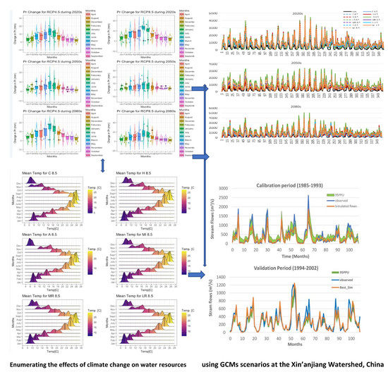
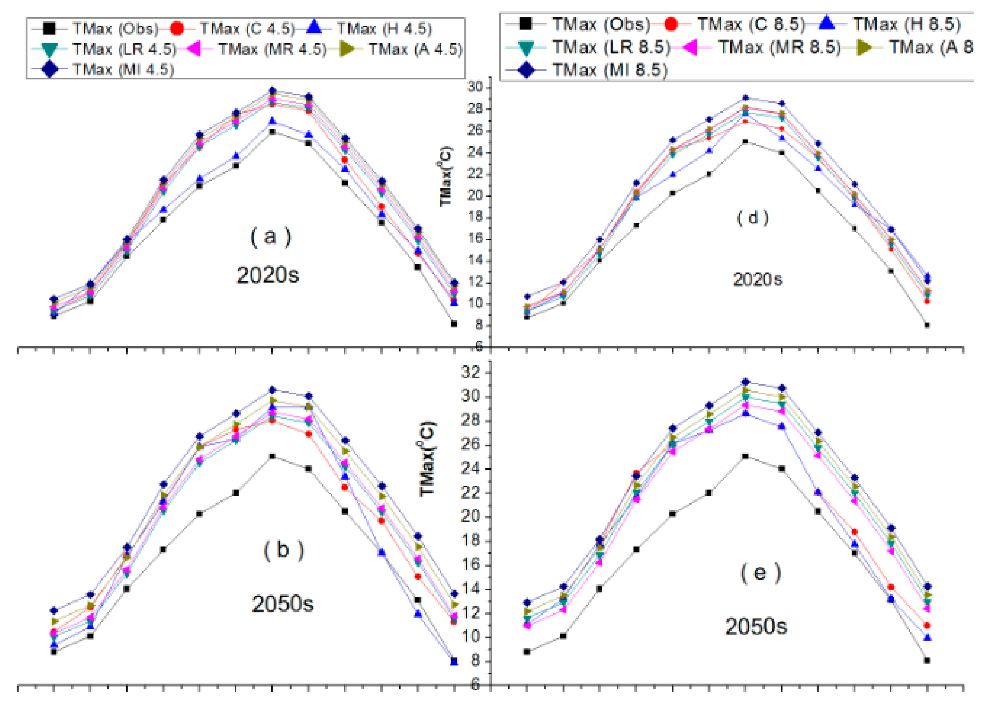
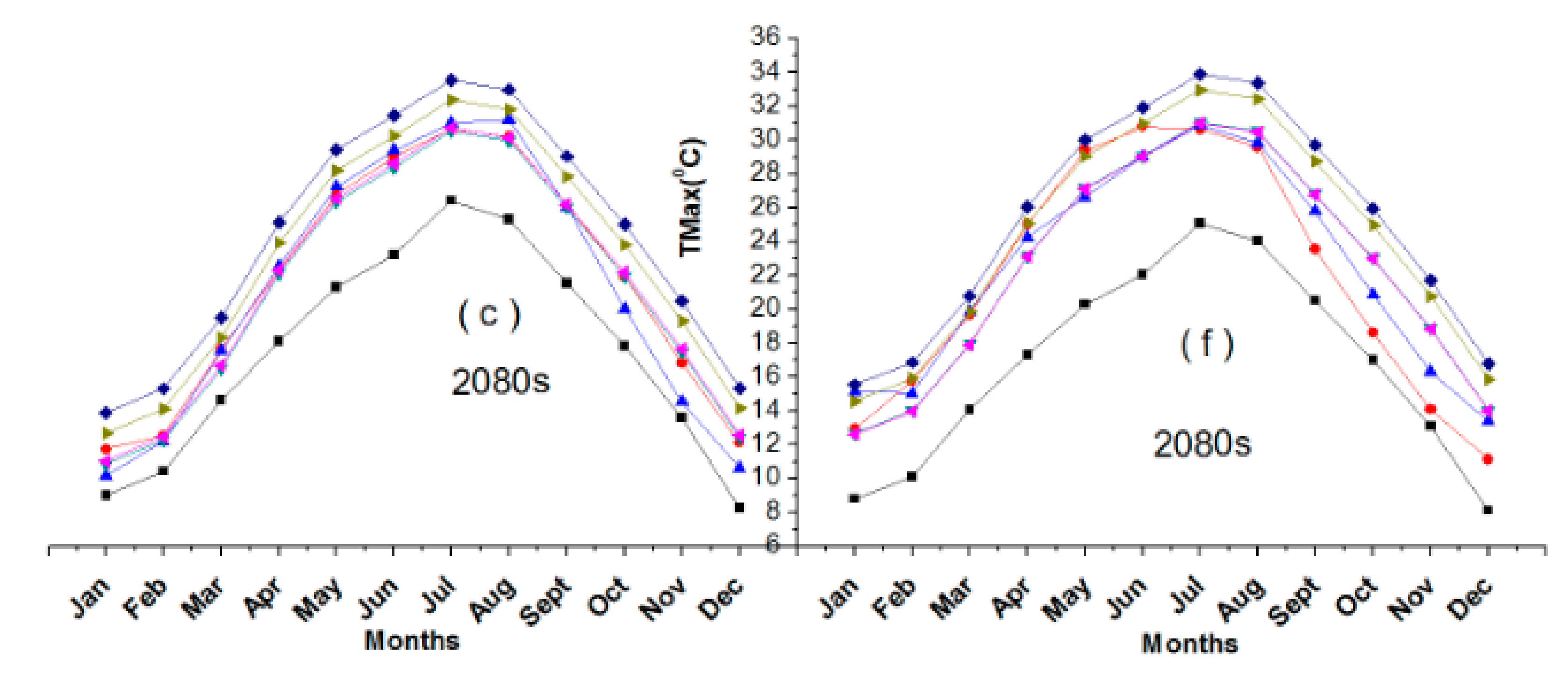
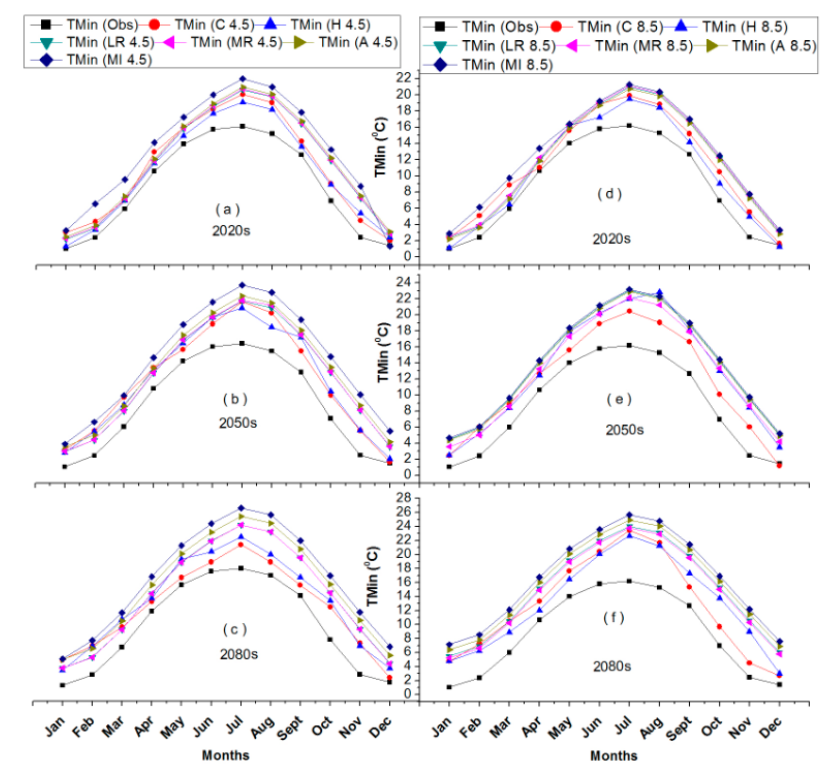
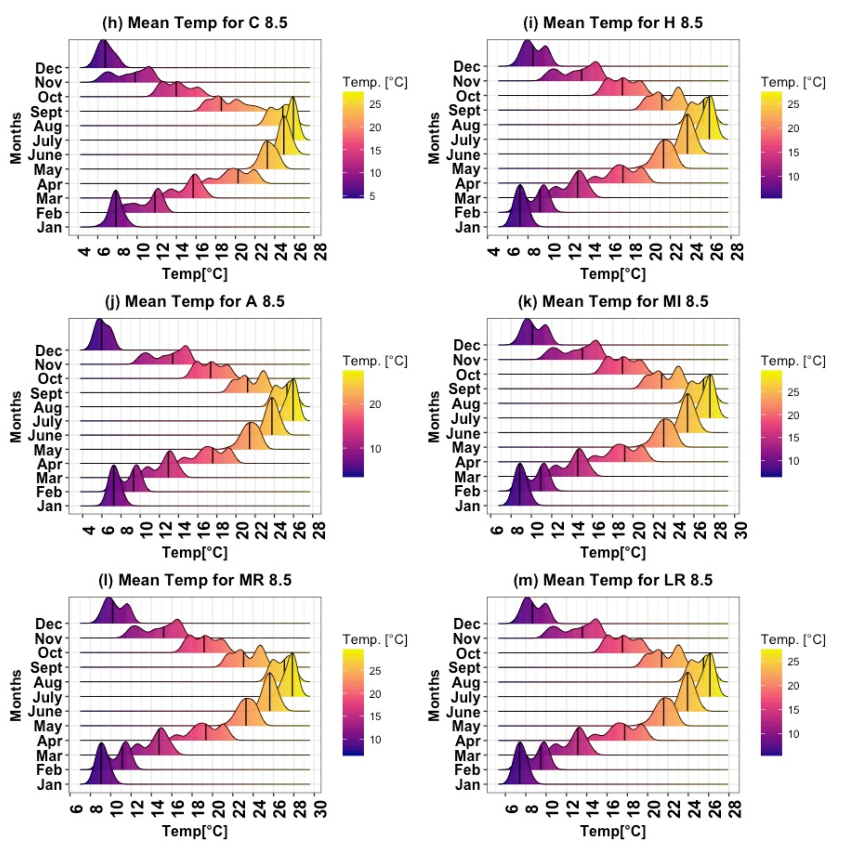
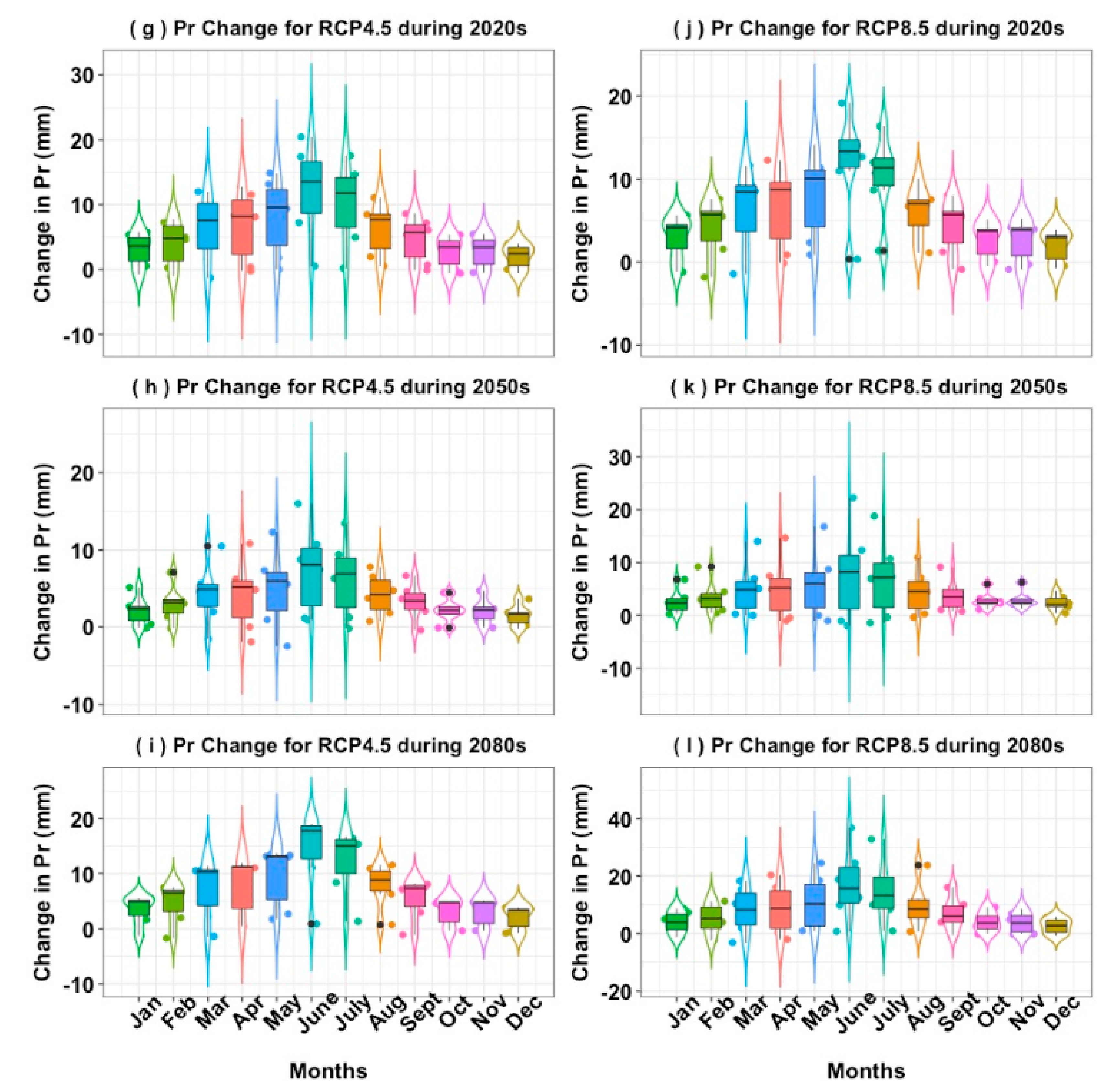
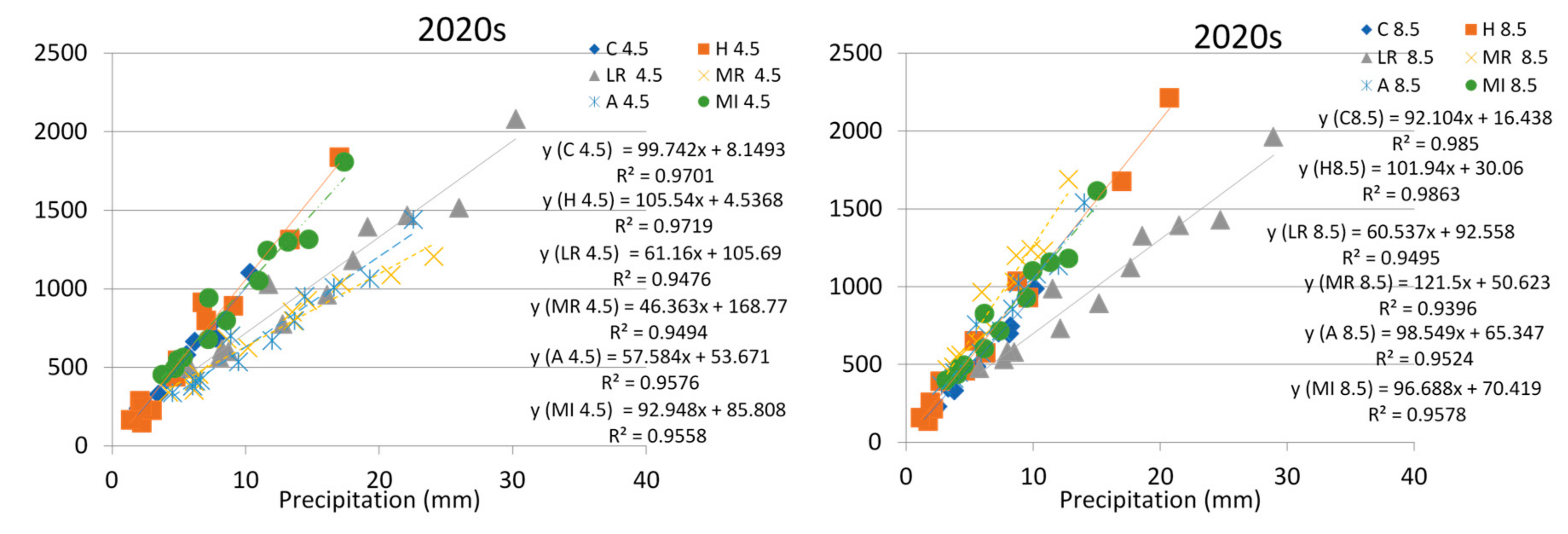
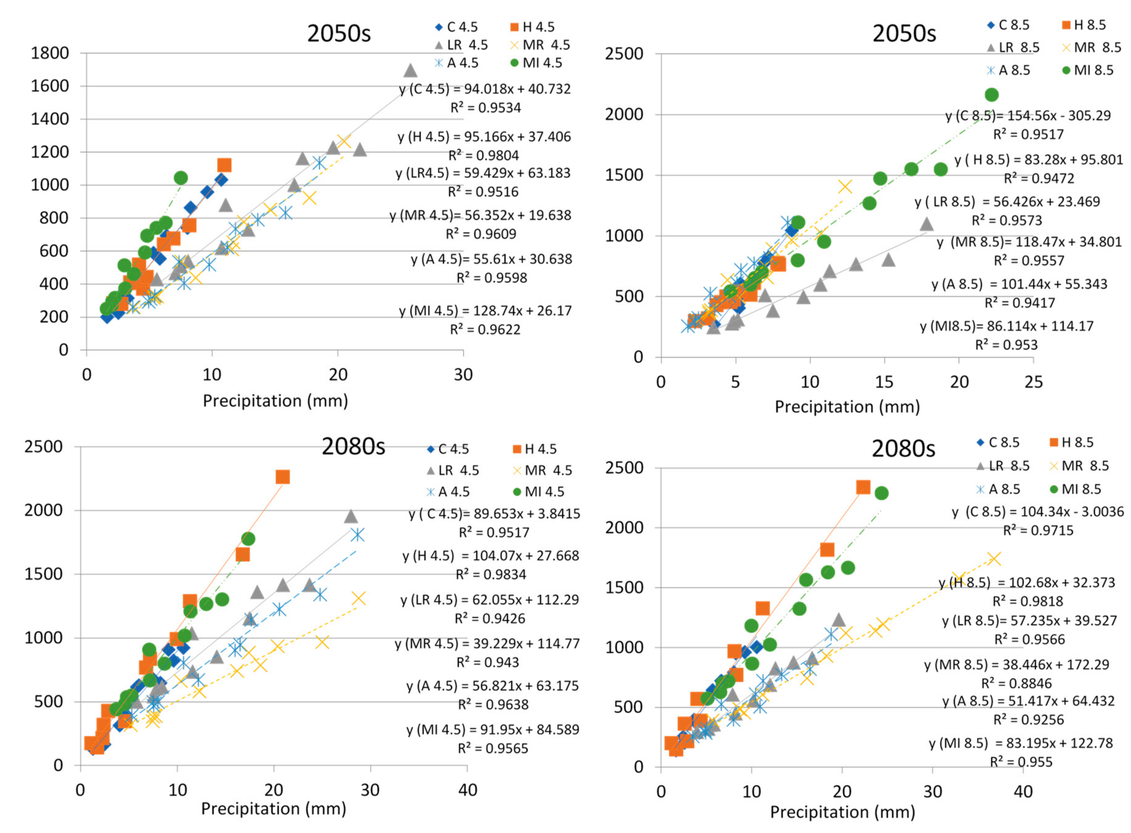
In the present study, six GCMs resulted in high differences in predicted maximum temperatures which range between 0.8 to 4.2 °C and 0.6 to 4.9 °C for RCP4.5 and RCP8.5, respectively. Similarly, the variability in the minimum temperature for different GCMs was observed between 1.1 to 4.1 °C and 0.9 to 4.8 °C under RCP4.5 and RCP8.5, respectively. 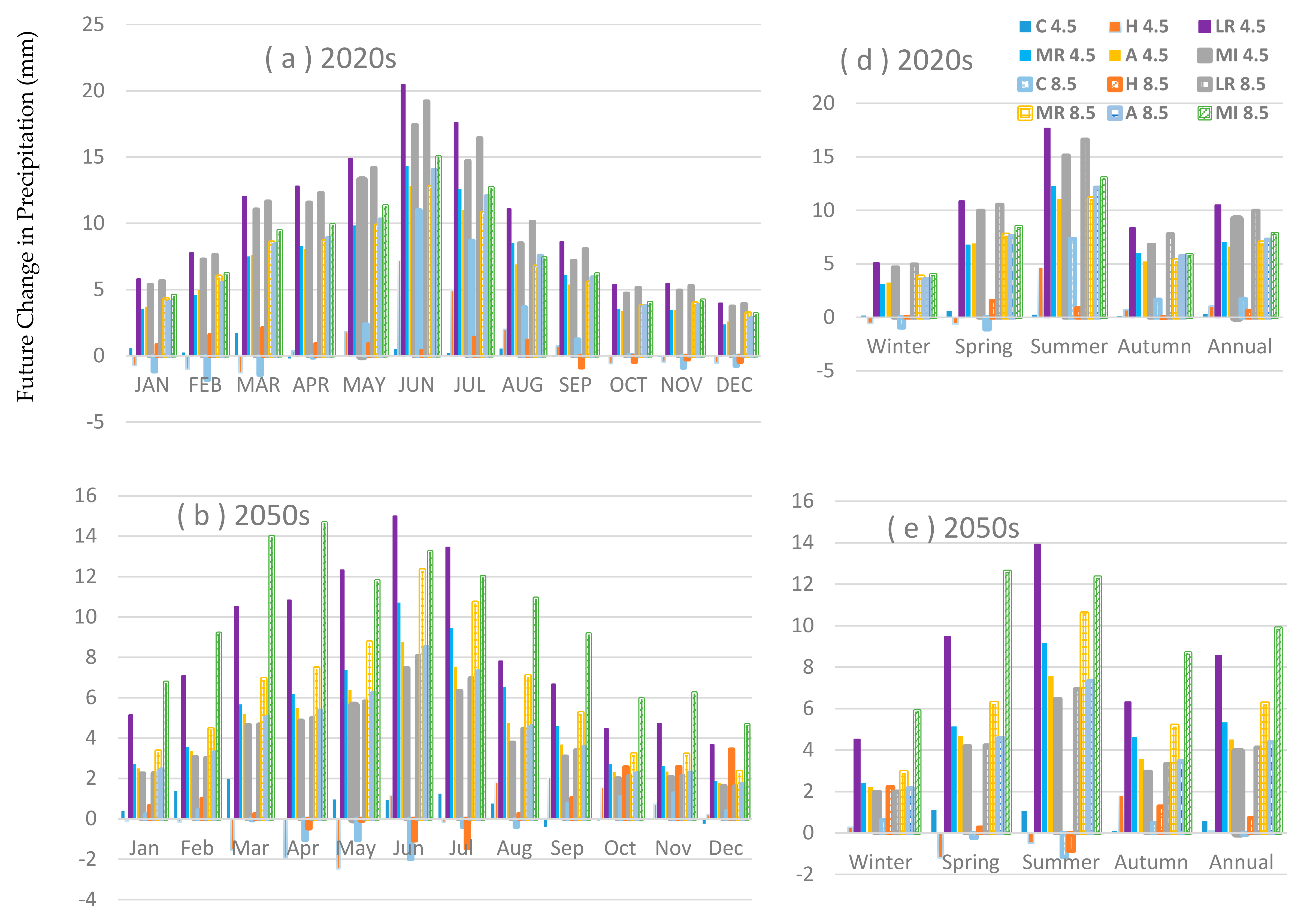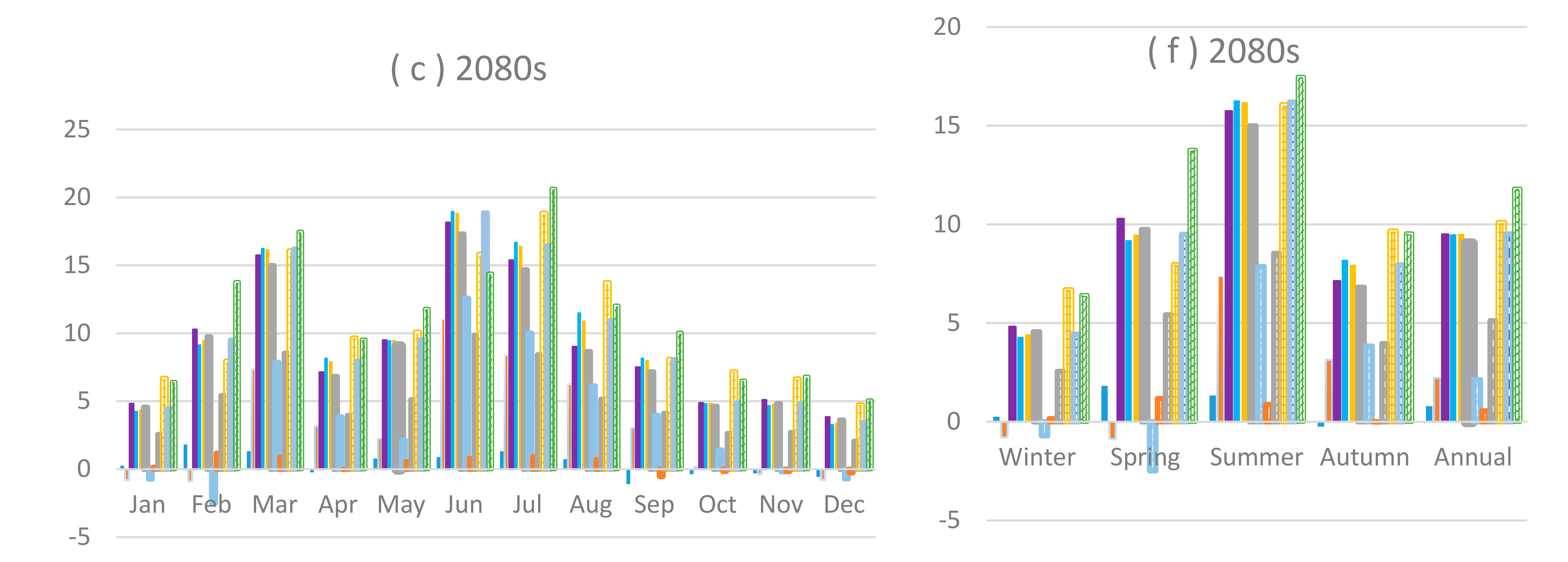The variation in projected mean monthly precipitation results under various GCMs is even larger (Figure 7). In this case, the variability in projected precipitation range from −0.44 to 20 mm and −0.6 to 15 mm during the 2020s and 2050s, for RCP4.5 and RCP8.5, respectively. A variation ranges from −1.1 to 18.8 mm was observed in mean monthly precipitation during the 2080s for different GCMs. According to [64], it is generally difficult to accurately project climatic variables, especially precipitation, and thus uncertainties in projected temperatures and precipitations could result in associated uncertainties for projected streamflows.

Based on the results of six GCMs under RCP4.5 and 8.5 scenarios, changes in the precipitation and temperature could influence directly or indirectly the water resources of the area and as these projected streamflows were used to predict the optimal future hydropower production. Therefore, these changes in streamflows impact the hydropower production of Xin’anjiang hydropower station, based on these GCMs projections. The projected GCMs show an increase in the precipitation amount in the study area compared to base years. The precipitation is strongly influenced by several circulation systems such as southerly moisture transport, East Asia Monsoon and anthropogenic affects. Southerly moisture transport and the interdecadal variation of the East Asian monsoon are key factors which can cause an increase in the precipitation amount in eastern China [84,85,86]. Another key factor behind the increase in the precipitation amount of eastern China is the temperature variability at the interdecadal and interannual timescales in high latitudes, such as Tibetan Plateau and nearby oceans [87,88]. These are the major reasons behind the increase in the precipitation amount and further investigated by climate modeling need to be carried out in the future to study this phenomenon in detail.

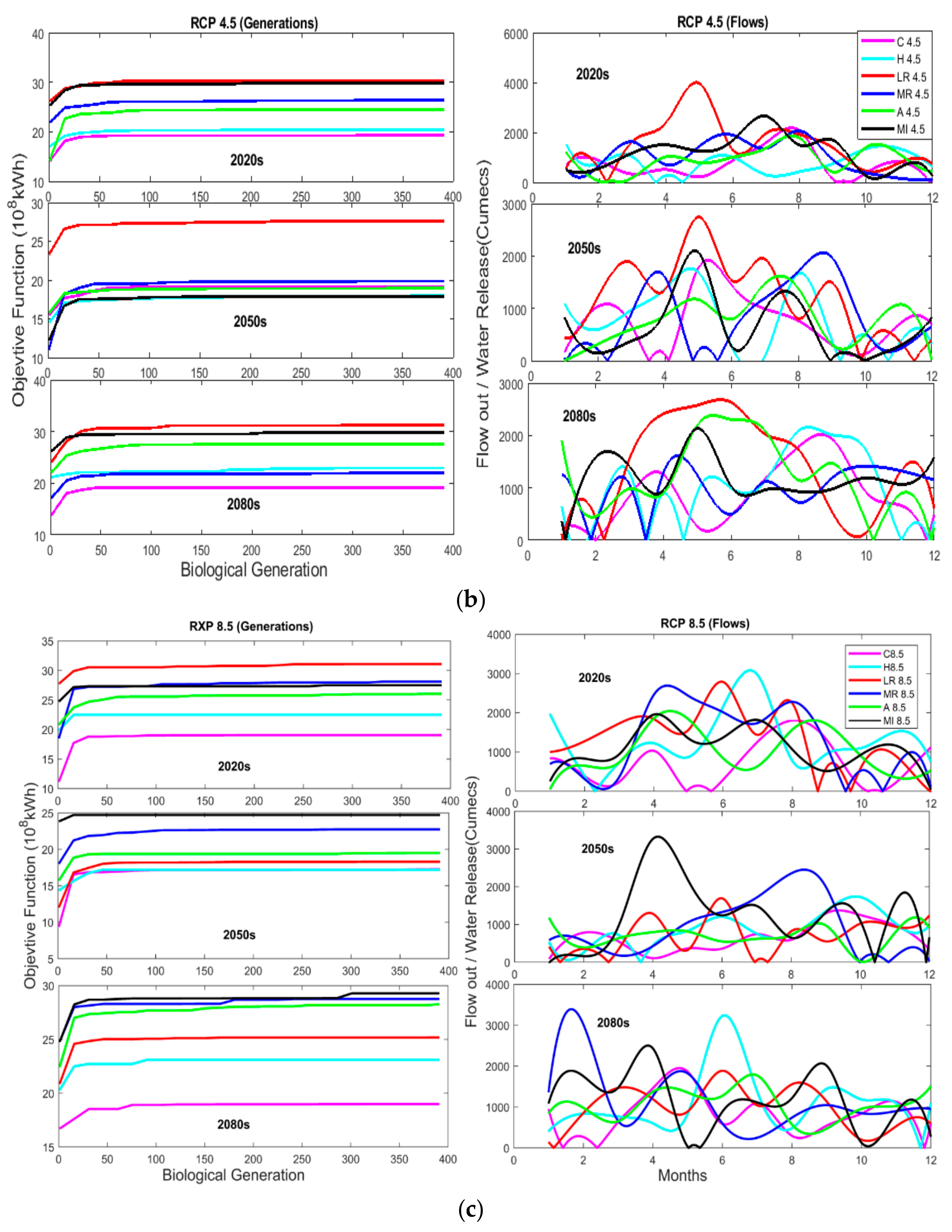
The projected GCMs shows an increment in the streamflows of the area with the increase in the precipitation amount. These projected flows are used for optimal electricity generation. Moreover, change in these streamflows directly affect electricity production. As was observed, the scenarios with a large amount of stream flow give maximum optimal electricity generation as given in Table 6. The results of this study are consistent with the results of precipitation and temperature as stated by [88,89]. The results are also consistent with the results found by [10,90]. The increasing trend of stream flows is consistent with the results found by [6] during the 20th century for the same region.

A major limitation of the present work is to ignore evaporation losses from the reservoir, water release from turbines and turbine efficiencies in accordance with hydropower generation due to unavailability of reliable data. The records of hydropower scheduling and generation were also unavailable; thus, the hydropower prediction was carried out based on the projected flows, the maximum and minimum reservior levels and reservior area and flow rating curve.Because of this, we were unable to compare the future and present hydropower generation curve due to the above-mentioned constraint, which could be carried out in the near future with the accessability of the data.

Although some techniques used in the presented work are similar to those found in the literature, we adopted a comparatively innovative method to study the impact of climate change on streamflows and possible ultimate change in hydropower generation in the area. The use of these projected streamflows for optimal hydropower generation makes this study entirely different to the work already published in the literature. These projected past and future streamflows could be useful for decision makers and water resource planners to make plans for the management of water resources. Some future water projections show a frightening rise in future flows, which can be helpful for water resource planners to manage the possible future water and to avoid flooding conditions in the area by improving management strategies and re-examining designs and operations of the existing dam. This study will also be beneficial in assessing the maximum optimal electricity generation against the future projected streamflows. The information of the future water resources in the area could be helpful for planning hydropower operations. The presented work shows that the selected optimization method is a dominant way to enhance reservoir performance. More benefits could be accomplished in the form of hydropower generation by following the optimal water release patterns for future flows as presented in this study. However, further research is essential to improve these methods before the complete implementation in the hydro-climatic and hydropower fields.

7. Conclusions and Recommendations

In the present study, we examined the future projections of climate change and their possible impacts on water resources in the Xin’anjiang watershed during the 21st century. Moreover, projected optimal electricity generation based on these future stream flows for the 2020s, 2050s and 2080s have also been investigated in this study. Six GCMs of CMIP5 were used under RCP4.5 and RCP8.5 scenarios to assess the future temperature, precipitation, stream flow and power generation in the study area. To achieve reliable precipitation, TMax and TMin data series under different climate change scenarios, we employed QM downscaling technique to downscale the future climate projections.

The calibrated SWAT hydrological model was applied to simulate projected future streamflows based on the downscaled outputs of QM downscaling technique. Furthermore, these projected streamflows have been used for the projected optimal electricity generation and we employed PSO techniques, along with a mathematical model, to investigate the optimal electricity generation. Finally, the influences of climate change on water resources and optimal electricity generation under six GCMs and RCP scenarios were comprehensively studied. The most prominent conclusion drawn from this study can be summarized as below:

(1)

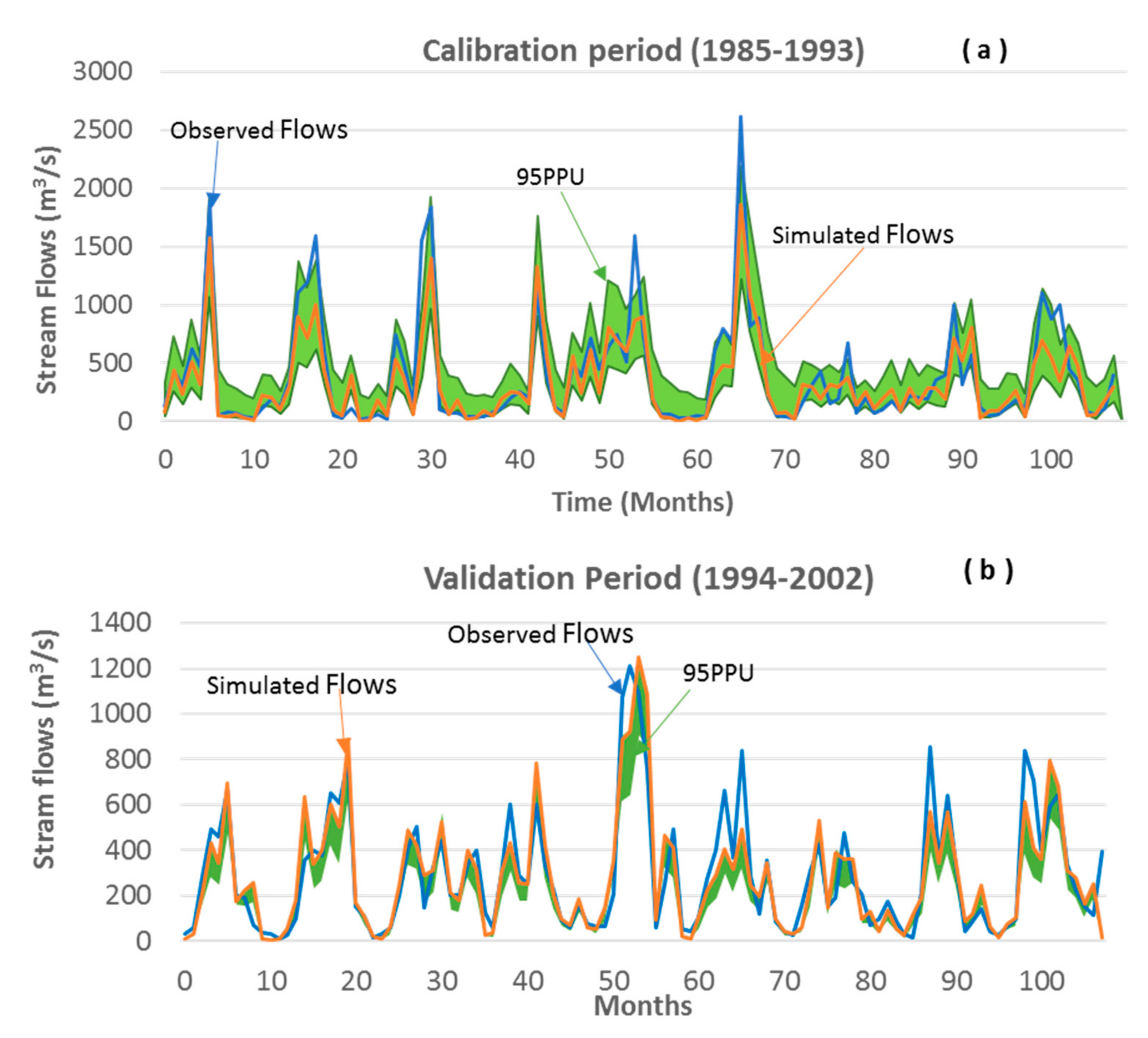
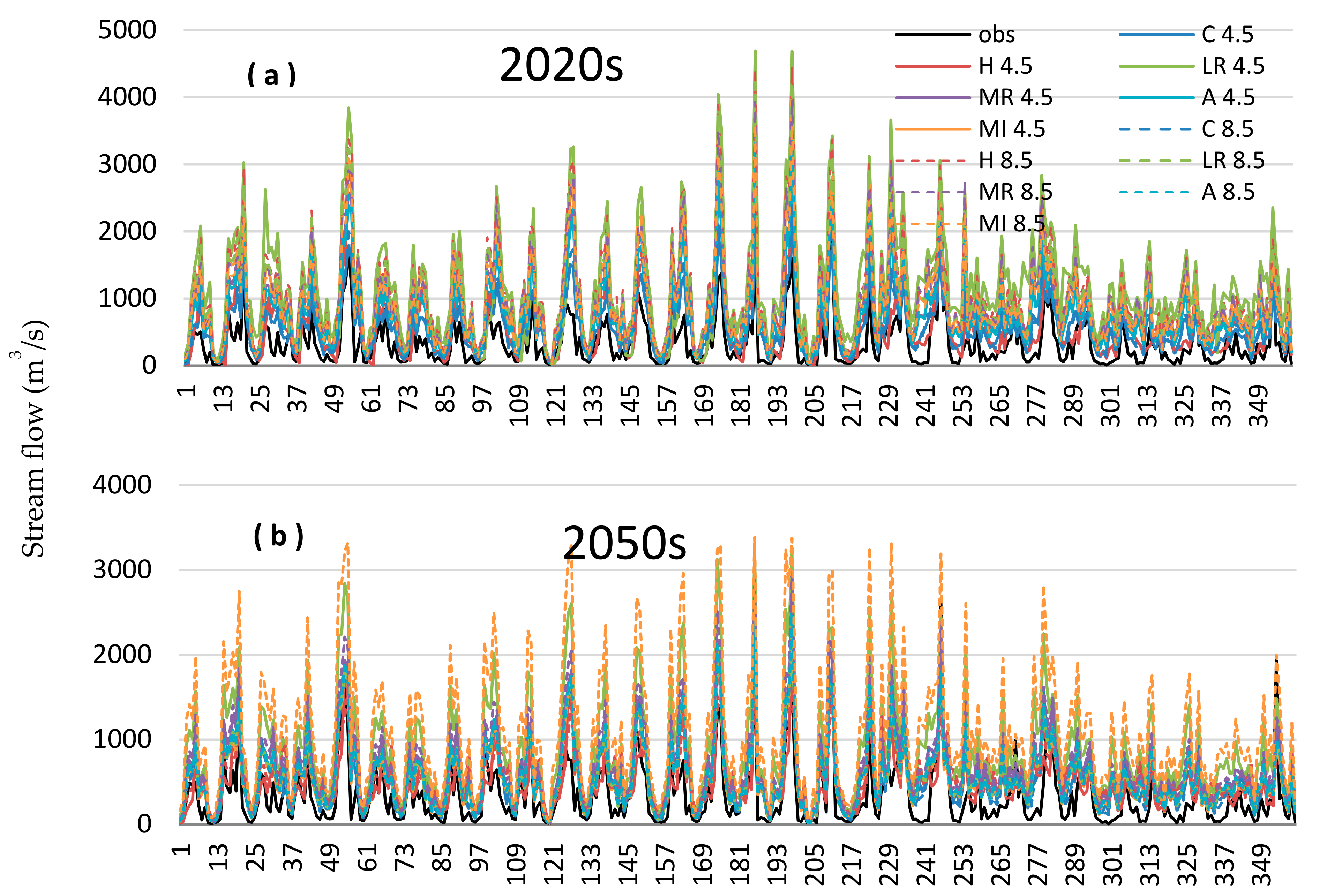
Calibration and validation of the SWAT indicated that evaluation indices e.g., NSE and R², were satisfactory within monthly timescale. The calibrated SWAT accurately reproduced stream flows in the Xin’anjiang watershed.

(2)

The downscaled results of the GCMs and RCPs showed that maximum and minimum temperature will continually increase in the future with a maximum increase during April to July. However, future projections of precipitations for six GCMs grow more uncertain and complex, for monthly and seasonal series shows overall increase in precipitation (except HadGEM2-ES, which shows decrease in monthly and seasonal series during some months and seasons) with maximum increase during the months of June and July for monthly series and in summer season for seasonal series. Overall, monthly and seasonal precipitation will apparently increase during this century with a maximum increase for the 2020s followed by 2080s, but 2050s appear to less increase in future precipitation amount. The average increase in precipitation for seasonal and monthly series is more significant under RCP4.5 as compared to RCP8.5 scenarios.

(3)

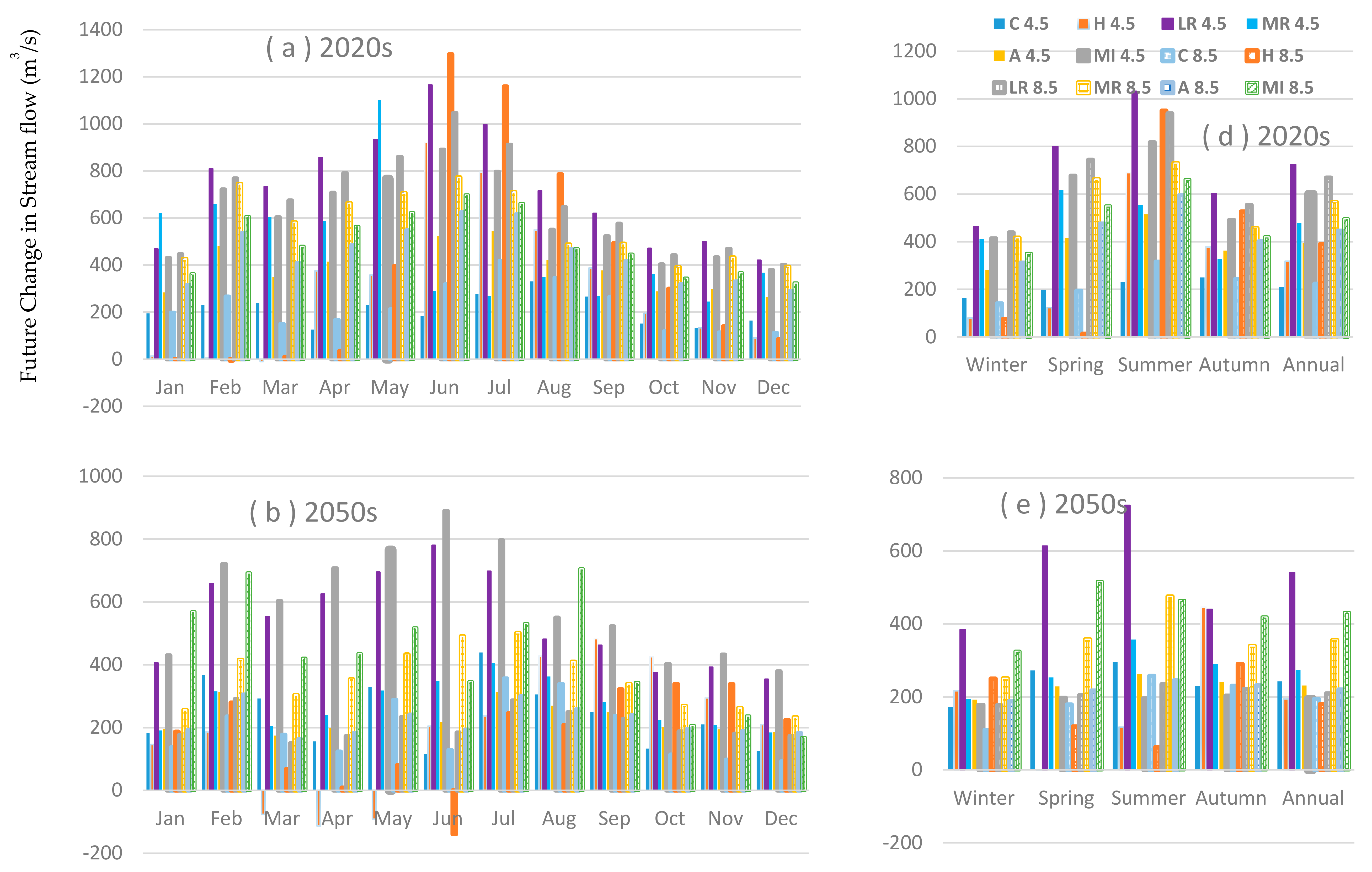
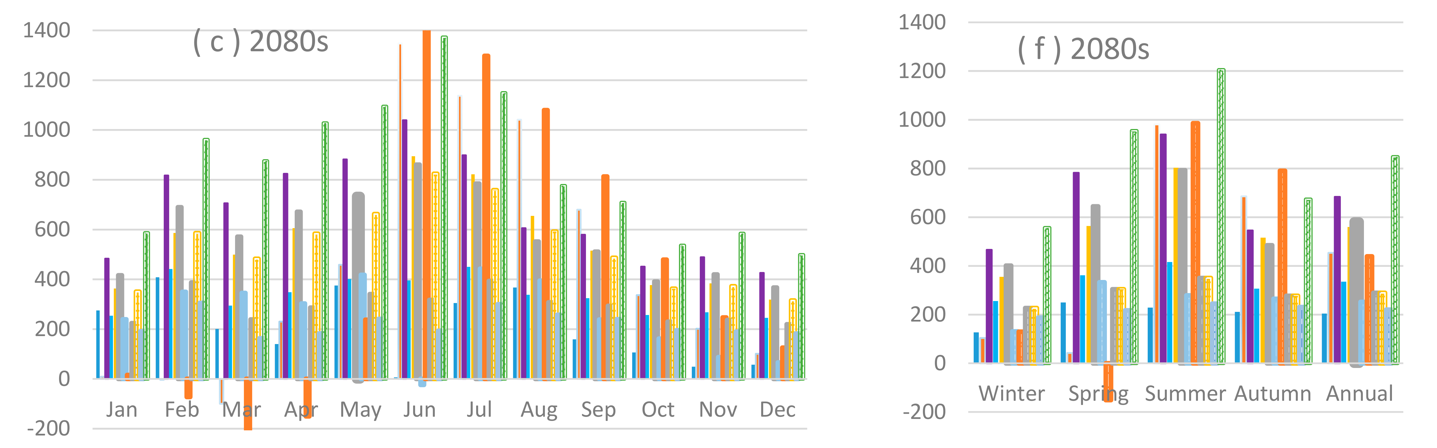
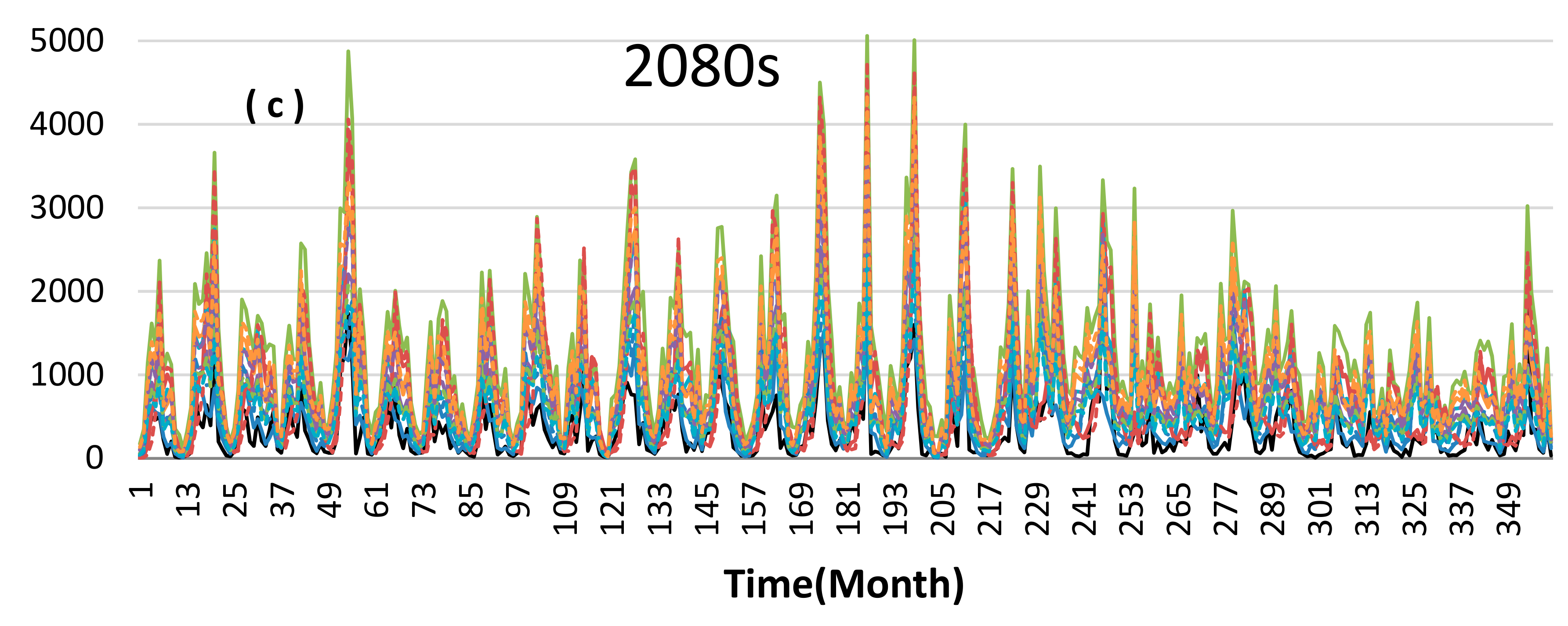
Six GCMs generated large magnitude increase in stream flows during summer and autumn than in winter and spring seasons. The average of six GCMs and RCPs for monthly series stated that mostly GCMs and RCPs exhibit increase in streamflow with maximum increase during June and July. The mean of multi GCMs and RCPs showed that stream flow exhibits a strong correlation with precipitation and clearly indicated that any change in stream flows is typically affected by simultaneous variations in precipitations. The results of streamflows indicated that maximum increase in the stream flow is during the 2020s and 2080s as precipitation amount increases, while the lesser increase is expected in precipitation and stream flows during 2050s. Moreover, MPI-ESM-LR generated the large magnitude of stream flows in the 21st century than any other GCMs.

(4)

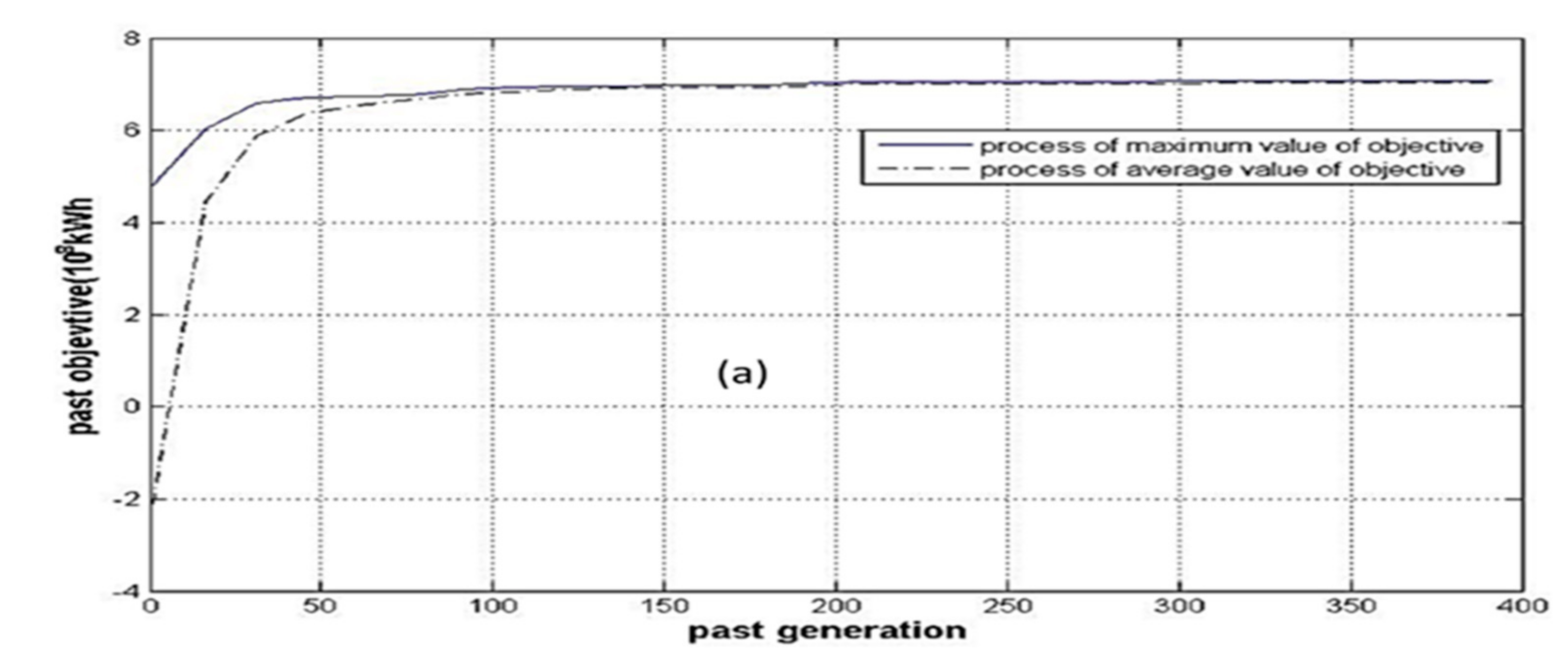
The ensemble optimization technique and mathematical model used for hydropower production for six GCMs under RCP scenarios can enhance the electricity amount than using the flows traditionally. The maximum amount of electricity generation is expected during the 2020s by optimal use of stream flows for GCMs. Results indicated that MPI-ESM-LR generated the maximum amount of electricity using 2020s flows under RCP8.5 and 4.5 followed by MIROC-ESM.

Therefore, based on these findings, a more assured GCMs ensemble scenario could be used to project the climatic parameters in the future. Nevertheless, further investigations of climate change scenarios is highly recommended to reduce the uncertainty from the future projections and explore the impact of climate change on optimal hydropower generation by considering the present hydropower production and scheduling.

References

1. Stocker, T. Change 2013: The Physical Science Basis: Working Group I Contribution to the Fifth Assessment Report of the Intergovernmental Panel on Climate Change; Cambridge University Press: Cambridge, UK, 2014. [Google Scholar]
2. Wang, G.Q.; Zhang, J.Y.; Jin, J.L.; Pagano, T.C.; Calow, R.; Bao, Z.X.; Liu, C.S.; Liu, Y.L.; Yan, X.L. Assessing water resources in China using PRECIS projections and a VIC model. Hydrol. Earth Syst. Sci. 2012, 16, 231–240. [Google Scholar] [CrossRef] [Green Version]
3. Solomon, S.; Intergovernmental Panel on Climate Change Working Group I. Climate Change 2007: The Physical Science Basis: Contribution of Working Group I to the Fourth Assessment Report of the Intergovernmental Panel on Climate Change; Cambridge University Press: Cambridge, UK, 2007. [Google Scholar]
4. Field, C.B.; Barros, V.R.; Intergovernmental Panel on Climate Change Working Group II. Climate Change 2014: Impacts, Adaptation, and Vulnerability: Working Group II Contribution to the Fifth Assessment Report of the Intergovernmental Panel on Climate Change; Cambridge University Press: Cambridge, UK, 2014. [Google Scholar]
5. Zhang, J.Y.; Wang, G. Impacts of Climate Change on Hydrology and Water Resources; Science Press: Beijing, China, 2007. (In Chinese) [Google Scholar]
6. Piao, S.; Ciais, P.; Huang, Y.; Shen, Z.; Peng, S.; Li, J.; Zhou, L.; Liu, H.; Ma, Y.; Ding, Y.; et al. The impacts of climate change on water resources and agriculture in China. Nature 2010, 467, 43–51. [Google Scholar] [CrossRef] [PubMed]
7. Ding, Y.; Ren, G.; Zhao, Z.; Xu, Y.; Luo, Y.; Li, Q.; Jin, Z. Detection, causes and projection of climate change over China: An overview of recent progress. Adv. Atmos. Sci. 2007, 24, 954–971. [Google Scholar] [CrossRef]
8. ECSNCCA. Second National Climate Change Assessment Report [Internet]. Beijing, 2011. Available online: http://unfccc.int/resource/docs/natc/chnnc2e.pdf (accessed on 2 February 2018).
9. Ding, Y.; Sun, Y.; Wang, Z.; Zhu, Y.; Song, Y. Inter-decadal variation of the summer precipitation in China and its association with decreasing Asian summer monsoon Part II: Possible causes. Int. J. Climatol. 2009, 29, 1926–1944. [Google Scholar] [CrossRef] [Green Version]
10. Wang, Y.; Zhou, L. Observed trends in extreme precipitation events in China during 1961–2001 and the associated changes in large-scale circulation. Geophys. Res. Lett. 2005, 32, L09707. [Google Scholar] [CrossRef]
11. Feng, L.; Zhou, T.; Wu, B.; Li, T.; Luo, J.-J. Projection of future precipitation change over China with a high-resolution global atmospheric model. Adv. Atmos. Sci. 2011, 28, 464–476. [Google Scholar] [CrossRef]
12. Xie, Z.-H.; Zeng, Y.-J.; Xia, J.; Qin, P.-H.; Jia, B.-H.; Zou, J.; Liu, S. Coupled modeling of land hydrology–regional climate including human carbon emission and water exploitation. Adv. Clim. Chang. Res. 2017, 8, 68–79. [Google Scholar] [CrossRef]
13. Ho, C.H.; Kim, J.H.; Lau, K.M.; Kim, K.M.; Gong, D.Y.; Lee, Y.B. Interdecadal Changes in Heavy Rainfall in China during the Northern Summer. Terr. Atmos. Ocean. Sci. 2005, 16, 1163–1176. [Google Scholar] [CrossRef]
14. Lieting, C.; Renguang, W. Interannual and decadal variations of snow cover over Qinghai-Xizang Plateau and their relationships to summer monsoon rainfall in China. Adv. Atmos. Sci. 2000, 17, 18–30. [Google Scholar] [CrossRef]
15. Zhou, T.; Gong, D.; Li, J.; Li, B. Detecting and understanding the multi-decadal variability of the East Asian Summer Monsoon Recent progress and state of affairs. Meteorol. Z. 2009, 18, 455–467. [Google Scholar] [CrossRef]
16. Wang, S.; Zhang, X.; Liu, Z.; Wang, D. Trend Analysis of Precipitation in the Jinsha River Basin in China. J. Hydrometeorol. 2013, 14, 290–303. [Google Scholar] [CrossRef]
17. Zhen, L.; Yan, Z.-W. Homogenized Daily Mean/Maximum/Minimum Temperature Series for China from 1960–2008. Atmos. Ocean. Sci. Lett. 2009, 2, 237–243. [Google Scholar] [CrossRef]
18. Xu, Z.; Liu, Z.; Fu, G.; Chen, Y. Trends of major hydroclimatic variables in the Tarim River basin during the past 50 years. J. Arid Environ. 2010, 74, 256–267. [Google Scholar] [CrossRef]
19. Xue, L.; Yang, F.; Yang, C.; Chen, X.; Zhang, L.; Chi, Y.; Yang, G. Identification of potential impacts of climate change and anthropogenic activities on streamflow alterations in the Tarim River Basin, China. Sci. Rep. 2017, 7. [Google Scholar] [CrossRef] [PubMed] [Green Version]
20. Luo, K.; Tao, F.; Moiwo, J.P.; Xiao, D. Attribution of hydrological change in Heihe River Basin to climate and land use change in the past three decades. Sci. Rep. 2016, 6. [Google Scholar] [CrossRef] [PubMed]
21. Xu, C. Climate Change and Hydrologic Models: A Review of Existing Gaps and Recent Research Developments. Water Resour. Manag. 1999, 13, 369–382. [Google Scholar] [CrossRef]
22. Kiely, G. Climate change in Ireland from precipitation and streamflow observations. Adv. Water Resour. 1999, 23, 141–151. [Google Scholar] [CrossRef]
23. Shen, Y.; Oki, T.; Utsumi, N.; Kanae, S.; Hanasaki, N. Projection of future world water resources under SRES scenarios: Water withdrawal/Projection des ressources en eau mondiales futures selon les scénarios du RSSE: Prélèvement d’eau. Hydrol. Sci. J. 2008, 53, 11–33. [Google Scholar] [CrossRef]
24. Arnell, N.W. Climate change and global water resources: SRES emissions and socio-economic scenarios. Glob. Environ. Chang. 2004, 14, 31–52. [Google Scholar] [CrossRef]
25. Su, B.; Huang, J.; Gemmer, M.; Jian, D.; Tao, H.; Jiang, T.; Zhao, C. Statistical downscaling of CMIP5 multi-model ensemble for projected changes of climate in the Indus River Basin. Atmos. Res. 2016, 178–179, 138–149. [Google Scholar] [CrossRef]
26. Leng, G.; Huang, M.; Tang, Q.; Leung, L.R. A modeling study of irrigation effects on global surface water and groundwater resources under a changing climate. J. Adv. Model. Earth Syst. 2015, 7, 1285–1304. [Google Scholar] [CrossRef] [Green Version]
27. Zeng, Y.; Xie, Z.; Zou, J. Hydrologic and Climatic Responses to Global Anthropogenic Groundwater Extraction. J. Clim. 2017, 30, 71–90. [Google Scholar] [CrossRef]
28. Christensen, J.; Hesselbjerg, B.; Hewitson, A.; Busuioc, A.; Chen, X.; Gao, R.; Held, R.J. Regional Climate Projections. In Climate Change, 2007: The Physical Science Basis. Contribution of Working Group I to the Fourth Assessment Report of the Intergovernmental Panel on Climate Change; Cambridge University Press: Cambridge, UK, 2007; Chapter 11; pp. 847–940. [Google Scholar]
29. Haerter, J.O.; Hagemann, S.; Moseley, C.; Piani, C. Climate model bias correction and the role of timescales. Hydrol. Earth Syst. Sci. 2011, 15, 1065–1079. [Google Scholar] [CrossRef] [Green Version]
30. Hayhoe, K.; Wake, C.; Anderson, B.; Liang, X.-Z.; Maurer, E.; Zhu, J.; Bradbury, J.; DeGaetano, A.; Stoner, A.M.; Wuebbles, D. Regional climate change projections for the Northeast USA. Mitig. Adapt. Strateg. Glob. Chang. 2008, 13, 425–436. [Google Scholar] [CrossRef]
31. Maurer, E.P.; Duffy, P.B. Uncertainty in projections of streamflow changes due to climate change in California. Geophys. Res. Lett. 2005, 32, L03704. [Google Scholar] [CrossRef]
32. Wood, A.W.; Leung, L.R.; Sridhar, V.; Lettenmaier, D.P. Hydrologic Implications of Dynamical and Statistical Approaches to Downscaling Climate Model Outputs. Clim. Chang. 2004, 62, 189–216. [Google Scholar] [CrossRef]
33. Maurer, E.P.; Ficklin, D.L.; Wang, W. Technical Note: The impact of spatial scale in bias correction of climate model output for hydrologic impact studies. Hydrol. Earth Syst. Sci. 2016, 20, 685–696. [Google Scholar] [CrossRef] [Green Version]
34. Basheer, A.K.; Lu, H.; Omer, A.; Ali, A.B.; Abdelgader, A.M.S. Impacts of climate change under CMIP5 RCP scenarios on the streamflow in the Dinder River and ecosystem habitats in Dinder National Park, Sudan. Hydrol. Earth Syst. Sci. 2016, 20, 1331–1353. [Google Scholar] [CrossRef] [Green Version]
35. Gudmundsson, L.; Bremnes, J.B.; Haugen, J.E.; Engen-Skaugen, T. Technical Note: Downscaling RCM precipitation to the station scale using statistical transformations—A comparison of methods. Hydrol. Earth Syst. Sci. 2012, 16, 3383–3390. [Google Scholar] [CrossRef]
36. Lafon, T.; Dadson, S.; Buys, G.; Prudhomme, C. Bias correction of daily precipitation simulated by a regional climate model: A comparison of methods. Int. J. Climatol. 2013, 33, 1367–1381. [Google Scholar] [CrossRef] [Green Version]
37. Maurer, E.P.; Das, T.; Cayan, D.R. Errors in climate model daily precipitation and temperature output: Time invariance and implications for bias correction. Hydrol. Earth Syst. Sci. 2013, 17, 2147–2159. [Google Scholar] [CrossRef]
38. Teutschbein, C.; Seibert, J. Is bias correction of regional climate model (RCM) simulations possible for non-stationary conditions? Hydrol. Earth Syst. Sci. 2013, 17, 5061–5077. [Google Scholar] [CrossRef] [Green Version]
39. Behera, S.; Panda, R.K. Evaluation of management alternatives for an agricultural watershed in a sub-humid subtropical region using a physical process based model. Agric. Ecosyst. Environ. 2006, 113, 62–72. [Google Scholar] [CrossRef]
40. Douglas-Mankin, K.R.; Srinivasan, R.; Arnold, J.G. Soil and Water Assessment Tool (SWAT) Model: Current Developments and Applications. Transactions of the ASABE. Am. Soc. Agric. Biol. Eng. 2010, 53, 1423–1431. [Google Scholar] [CrossRef]
41. van Griensven, A.; Breuer, L.; Di Luzio, M.; Vandenberghe, V.; Goethals, P.; Meixner, T.; Arnold, J.; Srinivasan, R. Environmental and ecological hydroinformatics to support the implementation of the European Water Framework Directive for river basin management. J. Hydroinform. 2006, 8, 239. [Google Scholar] [CrossRef]
42. Sun, H.; Cornish, P.S. Estimating shallow groundwater recharge in the headwaters of the Liverpool Plains using SWAT. Hydrol. Process. 2005, 19, 795–807. [Google Scholar] [CrossRef]
43. Mapfumo, E.; Chanasyk, D.S.; Willms, W.D. Simulating daily soil water under foothills fescue grazing with the soil and water assessment tool model (Alberta, Canada). Hydrol. Process. 2004, 18, 2787–2800. [Google Scholar] [CrossRef]
44. Ouyang, W.; Wang, X.; Fang, H.; Srinivasand, R. Temporal-spatial dynamics of vegetation variation on non-point source nutrient pollution. Ecol. Model. 2009, 220, 2702–2713. [Google Scholar] [CrossRef]
45. Gosain, A.K.; Rao, S.; Srinivasan, R.; Reddy, N.G. Return-flow assessment for irrigation command in the Palleru river basin using SWAT model. Hydrol. Process. 2005, 19, 673–682. [Google Scholar] [CrossRef]
46. Zaman, M.; Yuan, S.; Liu, J.; Ahmad, I.; Sultan, M.; Qamar, M.U.; Saifullah, M.; Adnan, M.; Anjum, M.N.; Nawaz, M.I.; et al. Investigating Hydrological Responses and Adaptive Operation of a Hydropower Station under a Climate Change Scenario. Pol. J. Environ. Stud. 2018, 27, 2337–2348. [Google Scholar] [CrossRef] [Green Version]
47. Huang, W.; Yuan, L. A drought early warning system on real-time multireservoir operations. Water Resour. Res. 2004, 40. [Google Scholar] [CrossRef] [Green Version]
48. Mousavi, S.; Karamouz, M. Fuzzy-state stochastic dynamic programming for reservoir operation. J. Water Resour. 2004, 130. [Google Scholar] [CrossRef]
49. Wurbs, R.A. Reservoir-System Simulation and Optimization Models. J. Water Resour. Plan. Manag. 1993, 119, 455–472. [Google Scholar] [CrossRef]
50. Ganji, A.; Karamouz, M.; Khalili, D. Development of stochastic dynamic Nash game model for reservoir operation II. The value of players’ information availability and cooperative behaviors. Adv. Water Resour. 2007, 30, 157–168. [Google Scholar] [CrossRef]
51. Labadie, J. Optimal operation of multireservoir systems: State-of-the-art review. J. Water Resour. Plan. Manag. 2004, 130, 93–111. [Google Scholar] [CrossRef]
52. Kucukmehmetoglu, M. A game theoretic approach to assess the impacts of major investments on transboundary water resources: The case of the Euphrates and Tigris. Water Resour. Manag. 2009, 23, 3069. [Google Scholar] [CrossRef]
53. Kennedy, J.; Eberhart, R. Particle Swarm Optimization. In Proceedings of the Proceedings of ICNN’95—International Conference on Neural Networks, Perth, WA, Australia, 27 November–1 December 1995. [Google Scholar]
54. Lima, C.A.S., Jr.; Lapa, C.M.F.; do NA Pereira, C.M.; da Cunha, J.J.; Alvim, A.C.M. Comparison of computational performance of GA and PSO optimization techniques when designing similar systems–Typical PWR core case. Ann. Nucl. Energy 2011, 38, 1339–1346. [Google Scholar] [CrossRef]
55. Rahi, O.; Chandel, A.; Sharma, M. Optimization of hydro power plant design by particle swarm optimization (PSO). Procedia Eng. 2012, 30, 418–425. [Google Scholar] [CrossRef]
56. Zaman, M.; Yuan, S.; Liu, J.; Ahmad, I.; Ali Buttar, N.; Saifullah, M.; Nawaz, M.I. Optimization of Mangla Hydropower Station, Pakistan, using Optimization Techniques. MATEC Web Conf. 2017, 136, 02010. [Google Scholar] [CrossRef]
57. Xu, Y.; Wang, S.; Bai, X.; Shu, D.; Tian, Y. Runoff response to climate change and human activities in a typical karst watershed, SW China. PLoS ONE 2018, 13, e0193073. [Google Scholar] [CrossRef] [PubMed]
58. Zeng, X.; Zhao, N.; Sun, H.; Ye, L.; Zhai, J. Changes and relationships of climatic and hydrological droughts in the Jialing River basin, China. PLoS ONE 2015, 10, e0141648. [Google Scholar] [CrossRef] [PubMed]
59. Gu, H.; Yu, Z.; Wang, G.; Wang, J.; Ju, Q.; Yang, C. Impact of climate change on hydrological extremes in the Yangtze River Basin, China. Stoch. Environ. Res. Risk Assess. 2015, 29, 693–707. [Google Scholar] [CrossRef]
60. Hu, X.; Lu, L.; Li, X.; Wang, J.; Guo, M. Land use/cover change in the middle reaches of the heihe river basin over 2000-2011 and its implications for sustainable water resource management. PLoS ONE 2015, 10, e0128960. [Google Scholar] [CrossRef] [PubMed]
61. Yang, P.; Xia, J.; Zhang, Y.; Hong, S. Temporal and spatial variations of precipitation in Northwest China during 1960–2013. Atmos. Res. 2017, 183, 283–295. [Google Scholar] [CrossRef]
62. Zhang, Y.; You, Q.; Chen, C.; Ge, J. Impacts of climate change on streamflows under RCP scenarios: A case study in Xin River Basin, China. Atmos. Res. 2016, 178–179, 521–534. [Google Scholar] [CrossRef]
63. Zaman, M.; Fang, G.; Saifullah, M.; Javed, Q. Seasonal and Annual Precipitation Trend Prediction in Xin’Anjiang China. Fresenius Environ. Bull. 2016, 25, 89–102. [Google Scholar]
64. Ouyang, F.; Zhu, Y.; Fu, G.; Lü, H.; Zhang, A.; Yu, Z.; Chen, L. Impacts of climate change under CMIP5 RCP scenarios on streamflow in the Huangnizhuang catchment. Stoch. Environ. Res. Risk Assess. 2015, 29, 1781–1795. [Google Scholar] [CrossRef]
65. Zhu, Y.; Lin, Z.; Wang, J.; Zhao, Y.; He, F. Impacts of Climate Changes on Water Resources in Yellow River Basin, China. Procedia Eng. 2016, 154, 687–695. [Google Scholar] [CrossRef]
66. Arnold, J.G.; Srinivasan, R.; Muttiah, R.S.; Williams, J.R. Large area hydrologic modeling and assessment part I: Model development. J. Am. Water Resour. Assoc. 1998, 34, 73–89. [Google Scholar] [CrossRef]
67. Cibin, R.; Chaubey, I.; Engel, B. Simulated watershed scale impacts of corn stover removal for biofuel on hydrology and water quality. Hydrol. Process. 2012, 26, 1629–1641. [Google Scholar] [CrossRef]
68. Te Chow, V.; Maidment, D.R.; Mays, L.W. Applied Hydrology; Tata McGraw-Hill Education: New Delhi, India, 2010. [Google Scholar]
69. Sloan, P.G.; Moore, I.D. Modeling subsurface stormflow on steeply sloping forested watersheds. Water Resour. Res. 1984, 20, 1815–1822. [Google Scholar] [CrossRef] [Green Version]
70. Arnold, J.G.; Allen, P.M. Automated methods for estimating baseflow and ground water recharge from streamflow records. J. Am. Water Resour. Assoc. 1999, 35, 411–424. [Google Scholar] [CrossRef]
71. George, H.; Hargreaves, G.H.; Zohrab, A.; Samani, Z.A. Reference Crop Evapotranspiration from Temperature. Appl. Eng. Agric. 1985, 1, 96–99. [Google Scholar] [CrossRef]
72. Jimmy, R.; Williams, J.R. Flood Routing with Variable Travel Time or Variable Storage Coefficients. Trans. ASAE 1969, 12, 100–103. [Google Scholar] [CrossRef]
73. Nash, J.E.; Sutcliffe, J.V. River flow forecasting through conceptual models part I—A discussion of principles. J. Hydrol. 1970, 10, 282–290. [Google Scholar] [CrossRef]
74. Moriasi, D.N.; Arnold, J.G.; Van Liew, M.W.; Bingner, R.L.; Harmel, R.D.; Veith, T.L. Model Evaluation Guidelines for Systematic Quantification of Accuracy in Watershed Simulations. Trans. ASABE 2007, 50, 885–900. [Google Scholar] [CrossRef]
75. Van Griensven, A.; Meixner, T.; Grunwald, S.; Bishop, T.; Diluzio, M.; Srinivasan, R. A global sensitivity analysis tool for the parameters of multi-variable catchment models. J. Hydrol. 2006, 324, 10–23. [Google Scholar] [CrossRef]
76. Abbaspoura, K.C.; Yanga, J.; Maximova, I.; Sibera, R.; Bognerb, K.; Mieleitnera, J.; Zobrista, J.; Srinivasanc, R. Modelling hydrology and water quality in the pre-alpine/alpine Thur watershed using SWAT. J. Hydrol. 2007, 333, 413–430. [Google Scholar] [CrossRef]
77. Arnold, J.G.; Moriasi, D.N.; Gassman, P.W.; KAbbaspour, K.C.; White, M.J.; Srinivasan, R.; Santhi, C.; Daren Harmel, R.; van Griensven, A.; Liew, M.; et al. SWAT: Model Use, Calibration, and Validation. Trans. ASABE 2012, 55, 1491–1508. [Google Scholar] [CrossRef]
78. Ma, L.; Ascough, J.C., II; Ahuja, L.R.; Shaffer, M.J.; Hanson, J.D.; Rojas, K.W. Root zone water quality model sensitivity analysis using monte carlo simulation. Trans. ASAE 2000, 43, 883–895. [Google Scholar] [CrossRef]
79. Willems, P.; Olsson, J.; Arnbjerg-Nielsen, K.; Beecham, S.; Pathirana, A.; Gregersen, I.B.; Madsen, H. Impacts of Climate Change on Rainfall Extremes and Urban Drainage Systems; IWA Publishing: London, UK, 2012; Volume 11. [Google Scholar] [CrossRef]
80. Library, W.O.; Tryhorn, L.; Degaetano, A. A comparison of techniques for downscaling extreme precipitation over the Northeastern United States. Int. J. Climatol. 2011, 31, 1975–1989. [Google Scholar] [CrossRef]
81. Teutschbein, C.; Seibert, J. Bias correction of regional climate model simulations for hydrological climate-change impact studies: Review and evaluation of different methods. J. Hydrol. 2012, 456–457, 12–29. [Google Scholar] [CrossRef]
82. Vonk, E. Dam Reoperation as an Adaptation Strategy for Shifting Patterns of Water Supply and Demand—A Case Study for the Xinánjiang—Fuchunjiang Reservoir Cascade, China. Master’s Thesis, University of Twente, Enschede, The Netherlands, 2013. [Google Scholar]
83. Knutti, R.; Sedláček, J. Robustness and uncertainties in the new CMIP5 climate model projections. Nat. Clim. Chang. Nat. Res. 2012, 3, 369–373. [Google Scholar] [CrossRef]
84. Qian, W.; Lin, X.; Zhu, Y.; Xu, Y.; Fu, J. Climatic regime shift and decadal anomalous events in China. Clim. Chang. 2007, 84, 167–189. [Google Scholar] [CrossRef]
85. Li, C.; He, J.; Zhu, J. A review of decadal/interdecadal climate variation studies in China. Adv. Atmos. Sci. 2004, 21, 425–436. [Google Scholar] [CrossRef]
86. Qian, W.H.; Qin, A. Precipitation division and climate shift in China from 1960 to 2000. Theor. Appl. Climatol. 2008, 93, 1–17. [Google Scholar] [CrossRef]
87. Fu, G.; Chen, S.; Liu, C.; Shepard, D. Hydro-climatic trends of the yellow river basin for the last 50 years. 2004, 65, 149–178. [Google Scholar] [CrossRef]
88. Zaman, M.; Fang, G.; Mehmood, K.; Saifullah, M. Trend Change Study of Climate Variables in Xin’anjiang-Fuchunjiang Watershed, China. Adv. Meteorol. 2015, 2015, 507936. [Google Scholar] [CrossRef]
89. Song, Y.; Achberger, C.; Linderholm, H.W. Rain-season trends in precipitation and their effect in different climate regions of China during 1961–2008. Environ. Res. Lett. 2011, 6. [Google Scholar] [CrossRef]
90. Tian, Y.; Xu, Y.; Booij, M.; Lin, S.; Zhang, Q. Detection of trends in precipitation extremes in Zhejiang, East China. Theor. Appl. 2012, 107, 201–210. [Google Scholar] [CrossRef]
Figure 1. (a) Digital elevation map along with locations of climatic and hydropower stations; (b) land use; (c) soil map of the study area (Maps are generated using GIS software and SWAT (http://swat.tamu.edu/software/arcswat/)).
Water 10 01296 g001
Figure 2. Work flow diagrame of SUFI2.
Water 10 01296 g002
Figure 3. Calibration (a) and validation (b) results for river flows using SWAT-CUP. (Blue line represents the Observed flows; Brown line represents the simulated flows and Green color represents the 95PPU).
Water 10 01296 g003
Figure 4. Comparison of mean monthly TMax among the observed and six GCM models, during 2020s (a), 2050s (b) and 2080s (c) for RCP4.5 and during, 2020s (d), 2050s (e) and 2080s (f) for RCP8.5.
Water 10 01296 g004aWater 10 01296 g004b
Figure 5. Comparison of mean monthly TMin among the observed and six GCM models, during 2020s (a), 2050s (b) and 2080s (c) for RCP4.5 and during 2020s (d), 2050s (e) and 2080s (f) for RCP8.5.
Water 10 01296 g005
Figure 6. Mean daily temperature (Temp) distribution for Six GCMs till the end of the 21st century for Base period (a), C 4.5 (b), H 4.5 (c), A 4.5 (d), MI 4.5 (e), MR 4.5 (f), LR 4.5 (g), C 8.5 (h), H 8.5 (i) A 8.5 (j), MI 8.5 (k), MR 8.5 (l) and LR 8.5 (m).
Water 10 01296 g006aWater 10 01296 g006b
Figure 7. Change in mean monthly (ac), seaosnal and annual (df) precipitation (Pr) for six GCMs under RCP4.5 and RCP8.5 scenarios. (gl) presents this change in the form of Box-plot and Violin plot. (Different colors for various months were selected for distinction, e.g., each month exhibits a unique color).
Water 10 01296 g007aWater 10 01296 g007bWater 10 01296 g007c
Figure 8. Change in monthly (ac), seaosnal and annual (df) streamflows for six GCMs under RCP4.5 and RCP8.5 scenarios.
Water 10 01296 g008aWater 10 01296 g008b
Figure 9. Comparison of Mean monthly (a) 2020s, (b) 2050s and (c) 2080s streamflow for six GCMs and RCPs with observed streamflows.
Water 10 01296 g009aWater 10 01296 g009b
Figure 10. Scatters plots of annual mean stream flows and annual mean precipitation for six GCMs under RCP4.5 and RCP8.5 scenarios.
Water 10 01296 g010aWater 10 01296 g010b
Figure 11. Total power generation and release of hydropower stations aimed at (a) base year, (b) six GCMs under RCP4.5 and (c) RCP8.5 scenarios for the rainy years flows using PSO.
Water 10 01296 g011aWater 10 01296 g011b