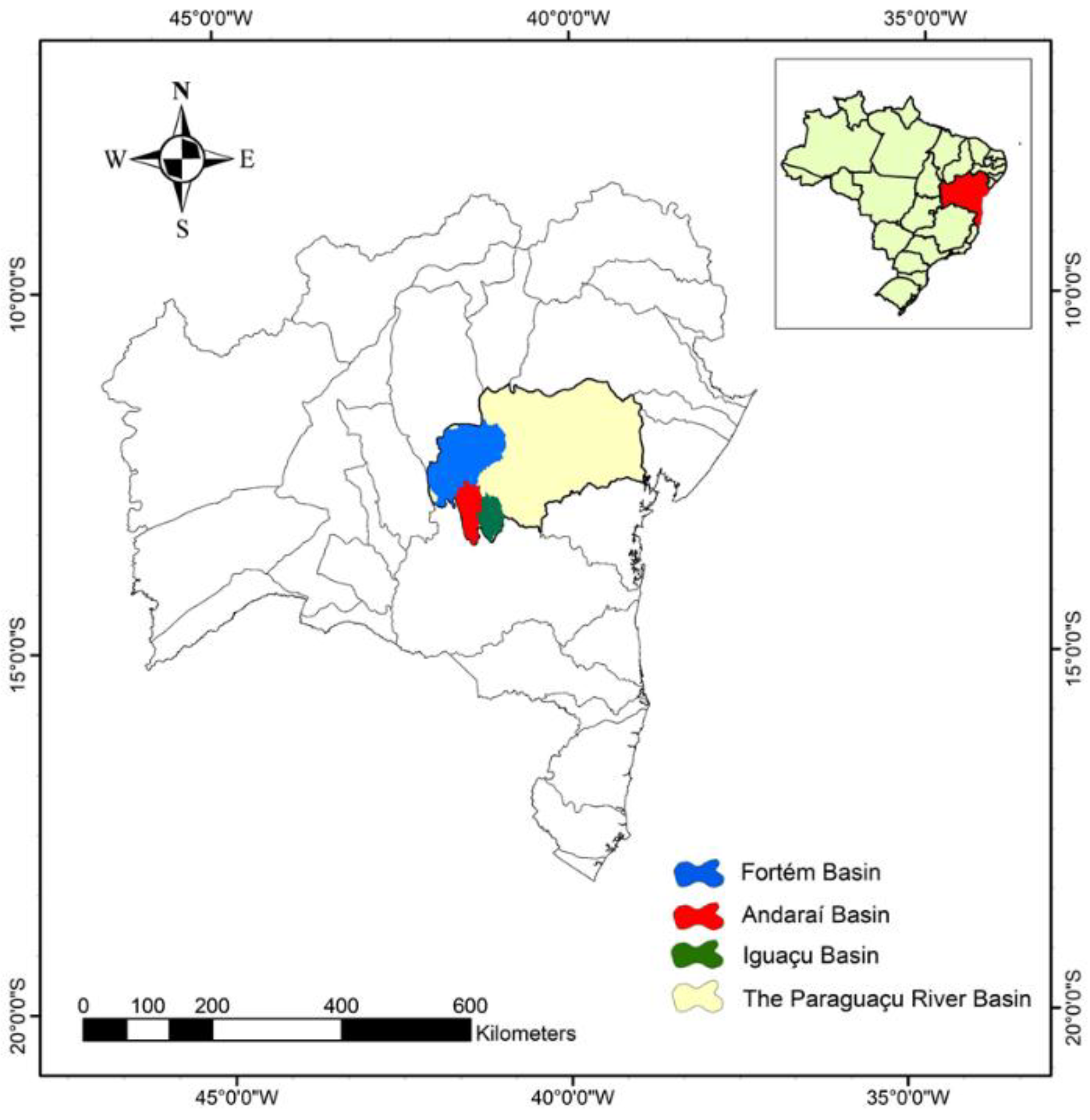
Article

Using a Hierarchical Approach to Calibrate SWAT and Predict the Semi-Arid Hydrologic Regime of Northeastern Brazil

1
Engineering Department, Instituto Federal da Bahia, Bahia 45030–220, Brazil
2
Centro de Ciência e Tecnologia do Ambiente e do Mar (MARETEC), Instituto Superior Técnico, Universidade de Lisboa, Lisboa 1049–001, Portugal
3
Instituto Superior Técnico, Universidade de Lisboa, Lisboa 1049–001, Portugal
*
Author to whom correspondence should be addressed.
Water 2018, 10(9), 1137; https://doi.org/10.3390/w10091137
Submission received: 13 July 2018 / Revised: 13 August 2018 / Accepted: 23 August 2018 / Published: 25 August 2018
(This article belongs to the Section Water Resources Management, Policy and Governance)

Abstract

:
The Paraguaçu watershed in northeastern Brazil faces increasing water scarcity, with water resources unable to meet the increasing demand. Accurate assessment of water availability is thus essential for efficient planning and management of local resources. In this work, the potential of the SWAT model for predicting daily and monthly variability of the hydrologic regime of the Paraguaçu River was assessed. Model calibration/validation followed: (i) A hierarchical framework; (ii) the assessment of maximum, average and minimum streamflow based on paired t-test and linear regression analysis; and (iii) the definition of permanence curves for streamflow with a probability of occurrence of 90% (Q90) and 95% (Q95). The goodness-of-fit indicators revealed a “satisfactory” model performance (model efficiency ranged from 0.42 to 0.83) when predicting streamflow in monitored sub-basins using a unique set of parameters for wet and dry conditions. The flow duration curves also showed that the model underestimated higher flows resulting from extreme events but performed well for flows with exceedance probabilities of <90%. The regression analysis and paired t-test demonstrated that the SWAT model can be used for estimating maximum, average and minimum monthly streamflow in a region where information is insufficient to support water authorities in the decision-making process. The SWAT model can thus be considered adequate for simulating monthly streamflow in the Paraguaçu watershed.

1. Introduction

The Paraguaçu watershed in northeastern Brazil faces increasing water scarcity due to population growth, agriculture consumption and climate change. The watershed is an essential part of Bahia’s fluvial system, with reservoirs supplying water to approximately 3.9 million people. Accurate assessment of streamflow at the watershed scale is of vital importance since the current seasonal and interannual discharge of the Paraguaçu River has not been able to meet the existing demand for water [1]. In this context, quantitative understanding of hydrological parameters (rainfall and streamflow) and their spatial and temporal variability are essential for an efficient planning and management of local water resources [2].
Hydrological modeling is normally considered as a powerful tool for accurately estimating water availability at the watershed scale. Physically-based hydrological models have shown to be particularly suitable for simulating basin response to changing conditions, including climate variability, land use and management practices [3,4,5]. The Soil and Water Assessment Tool (SWAT) [6] is here a good example, being widely applied to assess the impact of climate and land management on hydrological processes, including streamflow and sediment and nutrient dynamics at the watershed scale [7,8,9]. However, its application to the Brazilian semiarid region has been rather scarce, although interest has been rising in recent years.
The application of the SWAT model is often particularly challenging due to the need for calibrating a large number of parameters which aim to describe the processes under analysis. The most common approach used in model calibration is by optimizing its parameters until deviations between predictions and historical observation data are minimized. Validation then follows, with predictions being again compared with an independent dataset to assess the reliability of the optimized model parameters. Klemeš [10] discussed different validation tests and proposed a hierarchical testing framework in which different approaches are ordered according to the possibility of transferring model results to different land uses, climate and other forms of environmental changes. These calibration/validation tests are divided in four major categories: (i) The Split Sample test, in which the model is calibrated using data from a period and then applied with the same calibrated parameters for simulating a different period (validation); (ii) the Differential Split-Sample test, where the same approach is followed but data is divided in two periods with varying climate characteristics (e.g., high/low average precipitation); (iii) the Proxy-basin test, where the model is calibrated and validated in various sites, which may be in the same basin or not but with similar edapho-climatic characteristics; and (iv) the Proxy-Basin Differential Split-Sample test, which is applied in cases where the model is supposed to be both geographically and climatically (or land-use-wise) transposable.
While the SWAT model has been applied in many Brazilian watersheds, model calibration/validation has followed simple approaches that have limited its use in improving water resources management and planning at the watershed scale, namely in the Paraguaçu watershed. The choice of the hydrological model and the calibration/validation process is fundamental for the reliability of model results and for improving the decision-making process at the basin scale. It is necessary to emphasize that the longer the time interval used for calibrating/validating the model, the more reliable the results are [11]. This is especially true for studies of land use/cover and climate change conducted in semiarid regions where water resources management is even more critical and necessary. As such, few reliable studies exist for the Paraguaçu basin having carried out a comprehensive calibration and validation of the modeled processes, using different techniques and especially considering time periods of more than ten years.
The objective of this study was thus to verify the potential of the SWAT model for predicting the hydrologic regime and its possible use in the planning and management of streamflow in the Paraguaçu River basin. In this research, the SWAT model was calibrated/validated using different approaches: (i) The hierarchical scheme proposed by Klemeš [10]; (ii) the assessment of the maximum, average and minimum streamflow based on the paired t-test and linear regression analysis [12]; and (iii) the analysis of the permanence curve for the Q90 and Q95 flows. The evaluation techniques were tested in the three sub-basins of the Paraguaçu upstream region (Andaraím Fortém and Iguaçu), considering calibration/validation periods of not less than ten years and considering daily and monthly timescales. Results will allow improving water resources management and planning in the Paraguaçu watershed, with the calibration approach being transferable to other semiarid regions in the world.

2. Material and Methods

2.1. Study Area

The Paraguaçu watershed is located in the Bahia state, northeastern Brazil (Figure 1). The basin covers an area of 55,317 km2 (10.14% of the territory) and has an altitude ranging from 0 to 1800 m (11°17’–13°36’S; 38°50’–42°01’W). The Paraguaçu River is 614 km long, flowing in the west-east direction towards “Todos os Santos” bay. According to the Köppen classification, the climate in the Paraguaçu River Basin varies from semi-arid (BSh) in the central part (67% of the area) to equatorial (Af) in the west and southeast areas. As a result, annual rainfall varies between less than 600 mm in the former area to 1400 mm in the latter regions [13]. The Paraguaçu River further constitutes the most important fluvial system in the Bahia state and includes five reservoirs: Pedra do Cavalo (with a storage capacity of 5330 hm3), Bandeira de Melo (318 hm3), Apertado (204 hm3), França (59 hm3) and São José do Jacuípe (355 hm3).
The Paraguaçu watershed is composed of three regions: High, medium and low Paraguaçu River Basin. The study area was included in the high Paraguaçu (13,774 km2) region, being defined by three sub-basins: Andaraí (2313 km2), Iguaçu (2034 km2) and Fortém (9426 km2) (Figure 1). The Andaraí sub-basin is characterized by more intense agriculture activity than in the remaining sub-basins. The average annual precipitation value is also higher in Andaraí (866 mm) than in Fortém (788 mm) or Iguaçu (701 mm). The soil in the sub-basins are Ferrosols (77.15%), Lithic Leptosol (21.72%) and Regosols (1.14%) [14]. The main land-uses are pasture (26.0%), deciduous forest (21.0 %), cerrado (19.5%), caatinga (19.0%), mixed forest (13.0%) and agriculture (1.5%) (Table 1; Figure 2).

2.2. Soil and Water Assessment Tool

The SWAT (Soil and Water Assessment Tool) model version 2012 [6] was used to simulate the soil water balance between 1993 and 2012. SWAT is a continuous, time-dependent, long-term, physically based, semi-distributed model, developed to assess the impacts of climate and land management on hydrological processes, sediment loading and pollution transport. The hydrologic cycle is based on the computation of the daily water balance, as follows:
SW t = SW 0 + i = 1 t ( R day Q surf ET a Q deep Q gw )
where SWt is the final soil water content (mm), SW0 is the initial soil water content (mm), t is the simulation period (days), Rday is the precipitation (mm), Qsurf is the surface runoff (mm), ETa is the actual evapotranspiration (mm), Qdeep is the water drained into the deep aquifer (mm) and Qgw is the return flow (mm), all referring to day i.
The overall water balance is generated at the hydrologic response units (HRUs) level, that is, areas with the same land-use and soil characteristics [6]. In this study, potential evapotranspiration (ETp) rates were estimated using the Penman-Monteith method [15] and partitioned into potential plant transpiration (Tp) and potential soil evaporation (Ep) rates based on Ritchie [16]. Surface runoff was computed from daily precipitation using a modification of the Soil Conservation Service Curve Number (SCS-CN) method [17]. Groundwater recharge was estimated by combining a storage routing technique and a crack-flow model. The lateral flow was simulated using a kinematic storage method [6].

2.3. Model Data Inputs

The digital elevation model (DEM) was obtained from the Shuttle Radar Topography Mission (SRTM), with a spatial resolution of 30 m (Figure 3). Daily precipitation, maximum and minimum temperature, relative humidity, solar radiation and wind speed were used in model simulations for computing streamflow and evapotranspiration rates. Precipitation data were obtained from Agência Nacional de Águas (ANA), while the remaining weather variables were taken from the Instituto Nacional de Meteorologia (INMET) (Table 2). Quality control assessment for precipitation and streamflow data can be found in ANA [18]. The grid of meteorological variables from Xavier et al. [19] was also used due to the high rain spatial variability and a small number of pluviometric stations in the region. The daily discharge data at Andaraí, Iguaçu and Fortém hydrometric stations (Table 3) were obtained from Agência Nacional de Águas (ANA), while the extraction of water volumes from the river channel and reservoirs were taken from the Instituto de Meio Ambiente e Recursos Hídricos da Bahia [20]. The soil map (Figure 2) was downloaded from Empresa Brasileira de Pesquisas Agropecúarias [14], while the soil’s physical and chemical properties were collected from local literature [21,22,23,24]. The land cover map was obtained from Globcover 2009 [25]. The Brazilian Institute of Geography and Statistics—IBGE [26]—provided the crop information for the Mucugê and Ibicoará irrigated areas (Andarai basin) between 2004 and 2012. These regions represent the largest irrigated area of the Paraguaçu watershed.

2.4. Calibration and Validation

The SWAT model calibration/validation was carried out for daily and monthly timesteps, by comparing simulated and observed streamflows following a hierarchical approach proposed by Klemeš [10]. The following tests were performed:
(1) Split Sample Test: This test was carried out in the Andaraí basin. Two-time periods were selected for this analysis: a calibration period (1989–2001) and a validation period (2002–2013). Before, the model was warmed up using the data set from 1985–1988. This test included wet and dry years, being defined for civil years with average annual precipitation above and below the average for the 1989–2013 period (866 mm·year−1), respectively.
(2) Differential split-sample test: This test was also performed in the Andaraí basin and consisted of calibrating streamflow during wet years and validating it during dry years and vice versa. Two data periods were selected: the wet period from 2004–2006 and the dry period from 2007–2013. This test is required whenever a model is to be used for simulating the effect of climate change [27]. If the climatic change corresponds to a transition to a warmer wetter scenario, the model should be calibrated on a dry cool data set and then validated for the other extreme. Due to the temporal variation of the precipitation regime (Figure 4), the dataset chosen for the dry period included two years where precipitation was above the average (866 mm·year−1). A comparison between the first (2004–2006) and second (2007–2013) half of data series showed that the mean monthly precipitation decreased from 96 to 61 mm (Figure 4), corresponding to a reduction of 36%.
(3) Proxy–Basin Test: The Iguaçu and Fortém sub-basins were selected as having similar land use characteristics as those in Andaraí. The model was first calibrated in the Andaraí sub-basin and validated in Iguaçu and Fortém sub-basins. This test allowed to evaluate the model’s ability in predicting the impacts of land use changes in a region where flow data does not exist [10].
(4) Proxy–Basin differential split-sample Test: The model was first calibrated for wet conditions in the Andaraí sub-basin and then used to simulate streamflow for dry conditions in the Iguaçu basin and vice versa. Both watersheds share similar characteristics. The wet and dry years were identified from historical records, with the model being calibrated on three wet years (2004–2006) and validated on seven drier years (2007–2013) like before.
For each test, the SWAT model was calibrated by manually modifying one factor at a time with the aim of finding the set of factors that determined the best results in terms of global water balance in the basin (Table 4). The hydrograms were analyzed and the parameters that affected flow peaks and baseflow—that is, the behavior of the flow curve—were selected and modified until deviations between model outputs and measured flow data were minimized. The previously calibrated parameters were then validated by comparing results of simulations with an independent measurement set. Four commonly used goodness-of-fit indicators were used to evaluate model performance: the determination coefficient (R2), the percent bias (PBIAS), the ratio of the root mean square error to the standard deviation of measured data (RSR) and the Nash-Sutcliffe model efficiency (NSE) [28], as follows:
R 2 = [ i = 1 n ( O i O ¯ )   ( P i P ¯ ) ] 2 i = 1 n ( O i O ¯ ) 2 i = 1 n ( P i P ¯ ) 2
PBIAS = [ i = 1 n ( O i P i ) i = 1 n ( O ( i ) ) 100 ]
RSR = i = 1 n ( O i P i ) 2 i = 1 n ( O i P ¯ ) 2
NSE = 1 [ i = 1 n ( O i P i ) 2 i = 1 n ( O i O ¯ ) 2 ]
where P is the model simulated values, O is the observed data, the over bar describes the mean for the entire period of the evaluation, n is the number of data pairs and i = 1,2,…, n. R2 is an indicator of the strength of the relationship between the observed and simulated values and varies between 0 and 1. R2 values >0.5 are regarded as acceptable for model simulation [29]. The PBIAS measures the tendency of the simulated data to be larger or smaller than their observed counterparts. PBIAS values <10% are considered very good; values from 10% < PBIAS < 15% are considered good; values from ± 15% < PBIAS < 25% are considered satisfactory and ≥25% are unsatisfactory [29]. RSR incorporates the benefits of error index statistics and includes a scaling/normalization factor, so that the resulting statistic and reported values can apply to various constituents. RSR varies from the optimal value of 0, which indicates zero RMSE or residual variation and therefore perfect model simulation, to a large positive value. For monthly values, RSR values ≤0.5 are considered very good; values from 0.50 < PBIAS < 0.60 are considered good; values from 0.60 < PBIAS < 0.70 are considered satisfactory; and values >0.70 are considered unsatisfactory [29]. The NSE is a normalized statistic that determines the relative magnitude of the model variance compared to the measured data variance, ranging from 1 to −∞. A NSE value of 1 corresponds to the best fit between simulated and measured data; values >0.75 are considered excellent; values between 0.36 and 0.75 are considered satisfactory; and values <0.36 are unsatisfactory [29].
Additionally, streamflow data was submitted to the Kolmogorov-Smirnov (p < 0.05) normality test. Considering that the data presented normal distribution, the parametric T-paired test was used to verify the hypothesis that the observed and simulated flow data did not present a significant difference between them (p < 0.05) [12]. The data analysis further consisted of comparing simulated and observed streamflow values within each quartile to assess the ability of the model in describing the maximum, average and minimum streamflow. Governmental institutions generally use the first quartile (the lowest 25% of monthly streamflow) as a reference in assessing water resource availability for multiple uses.

3. Results and Discussion

3.1. Model Calibration and Validation

Table 4 lists the default and calibrated parameters used in model simulations of the water balance in the Paraguaçu River basin. The SWAT model was shown to be highly sensitive to surface runoff parameters (CN2, SOL_AWC, SOL_Z and SOL_K), in line with Neitsch et al. [6], who stated that these were some of the most sensitive parameters for river discharge simulations. The available water capacity of the soil layer (SOL_AWC), saturated hydraulic conductivity (SOL_K) and soil depth (SOL_Z) influenced soil moisture and thus surface runoff. The CN2 default values of 35–89 were calibrated to the range 45–78, which is still in line with USDA-SCS [17]. The greatest uncertainties were found in soil parameters due to the large spatial variability observed in the basin as well as the difficulties in obtaining accurate and reliable soil information; a common limitation in most regions of the world. For example, SOL_K was made to vary between 2–35 mm/h, while SOL_AWC suffered a relative large change with inputs being considered reliable nonetheless as soils in the region have coarse to medium textures in the top layers [14]. The calibration of groundwater flow and baseflow ended up being controlled by groundwater delay (GW_DELAY), revaporation coefficient (GW_REVAP) and deep aquifer recharge (GW_RCHRG_DP) parameters. Reducing GW_DELAY affected both the width of the peak discharge and quantity of water available for base flow [6]. GW_REVAP controlled the amount of water moving from the shallow aquifer to the root zone as a result of soil moisture depletion and the amount of direct groundwater uptake from deep-rooted trees and shrubs [6]. GW_RCHRG_DP controlled percolation from the root zone to the deep aquifer. Finally, the effective hydraulic conductivity of the main channel (CH_K2) governed the movement of water from streambed to the subsurface for ephemeral or transient streams, which, according to Veith et al. [30], is a highly sensitive parameter when the watershed is characterized by intense and inconsistent precipitation events like in the Andaraí sub-basin. Nonetheless, despite a relatively extensive model calibration, all parameters were adjusted within their physical meaning, indicating the reasonability of model inputs.

3.1.1. Split-Sample Test

The Split-Sample Test was carried out by first separating different time periods for calibration and validation purposes. For daily and monthly scales, the dataset was split in half (Figure 5), with the first 50% intending for calibration (1989–2001) while the remaining 50% being left for validation (2002–2013). Simulation started on January 1985 and included four years for model warmup.
Overall, the performance of the SWAT model was satisfactory, although underestimating streamflow peaks both during calibration and validation. The largest difference was found on March 2011, where the model simulated values of 16.0 m3/s while the observed ones reached 68.0 m3/s, that is, producing an error of 328% for that day. The underestimation of streamflow peaks was associated with the type of rainfall and representation of its spatial and temporal distribution. According to Vieira et al. [31], the precipitation that occurs in the region is orographic due to the high elevation observed in some areas of the watershed, while Cho et al. [32] refers that the sparse and heterogeneous spatial distribution of rain gauges often results in inaccurate precipitation inputs for SWAT, especially when modeling large river basins or those with different complex terrains like mountainous regions, where the assumption of spatially uniform rainfall is not valid.
For the Andaraí sub-basin, the NSE values calculated from daily results were 0.49 and 0.42, while the monthly data produced values of 0.86 and 0.76 for the calibration and validation periods, respectively (Table 5). These values suggest a satisfactory model performance for daily predictions and an excellent performance for monthly estimates [29]. The R2 values were above 0.5, indicating that the model explained the variability of the observed daily and monthly data. The PBIAS indicated slight deviations between the mean simulated and observed streamflow, showing that the model underestimated by 10% and 3–6% the daily and monthly observations during the calibration and validation periods, respectively. However, the RSR resulted in very good indicators (RSR < 0.5) for monthly flows. For daily simulations, RSR values were higher than 0.7. Thus, the performance of the SWAT model in estimating the mean streamflow showed to be excellent for monthly flows, with all goodness-of-fit indicators being also within the range of values reported in the literature for similar applications using this model [33,34]. As such, the model could be considered fit for improving management of streamflow in the Paraguaçu watershed.

3.1.2. Differential Split-Sample Test

The primary requirement of the Differential split-sample test is a long record of simulation data from which different periods can be chosen which different historical conditions. For this test, the model adequately represented the behavior of the observed flows, underestimating peaks during both calibration and validation periods though (Figure 6), in line with existing literature [35,36]. The NSE values reached 0.47 and 0.50 for daily results and 0.83 and 0.63 for monthly outputs during the calibration and validation periods (Table 6), respectively, which means that the model was again found appropriate for simulating streamflow. Concerning the PBIAS, the model overestimated streamflow by 2–3% during wetter years (calibration) and underestimated streamflow by 17–20% during drier years (validation). Likewise, the RSR produced very good results for the monthly dry period but only satisfactory for the drier one. Nonetheless, the model was considered to operate under wet and dry conditions within acceptable margins of error. Muleta [37] revealed that SWAT–calibrated parameters for the headwaters of the Little River watershed were largely different between dry and wet periods. Li et al. [38] using another model found that model efficiency in the dry period was consistently lower than that in the wet period. Finally, Lévesque et al. [39] followed the seasonal calibration scheme in which winter and summer data were used to calibrate the model in two watersheds in southeastern Canada. Those authors reported that the best performance was obtained in the dry period using summer observations to calibrate the model; however, when the wet period observations were used, no advantage was achieved compared with the traditional calibration method based on all available data. Regarding the Andaraí sub-basin, calibrated parameters were found to be conservative while applying for wet or dry periods.

3.1.3. Proxy-Catchment Test

The Proxy-catchment test returned NSE values (Table 7) ranging from 0.44 (Iguaçu) to 0.36 (Fortém) for daily outputs, while monthly results produced NSE values ranging from 0.75 (Iguaçu) to 0.80 (Fortém). The daily and monthly PBIAS values ranged from 10–12% and 8.5–9.1% in Fortém and Iguaçu, respectively, indicating an underestimation of observed data in both basins. The RSR values showed again very good simulations of monthly flows. Thus, the model had an overall good satisfactory in Iguaçu and Fortém concerning monthly calibration data and an excellent performance to monthly validation data [29].

3.1.4. Proxy-Catchment Differential Split-Sample Test

This test was performed in the same catchments as in the previous test. Table 8 shows the satisfactory performance of the SWAT model for simulating streamflow in dry and wet periods. The monthly PBIAS values ranged from 8–21% in wet and dry periods, respectively, indicating always an underestimation of observed data. RSR values oscillated between very good and satisfactory results. On the other hand, the NSE values varied between 0.50 and 0.80, indicating an acceptable model performance.

3.1.5. Soil Water Balance

After model calibration, the soil water balance was assessed to confirm the reliability of model estimates in the three simulated sub-basins (Table 9). Annual actual evapotranspiration was the main component of the soil water balance due to the characteristics of the semi-arid climate, varying between 69 and 86% of the total annual precipitation amount, in line with other semi-arid regions in the world [5,40,41,42]. ETa values further varied according to land use (Table 10) and obviously water availability. The highest ETa values were observed in Andaraí and Fortém due to the highest precipitation values registered. Yet, large variability was observed in ETa values, in line with precipitation. Runoff varied between 3.6 and 11.2% of the total annual precipitation amount, being fundamentally registered during storm events. Baseflow and lateral flow reached 7.4 to 14.3% of the total annual precipitation amount, being essential for maintaining river flow throughout the year. Similar results can be found in Bouraoui et al. [43].

3.2. Estimate of Maximum, Average and Minimum Monthly Streamflow

Figure 7 shows results of the regression analysis between monthly simulated and observed streamflow from the 1989—2013 period, with data separated by quartiles. The regression coefficient evidenced that the model tended to overestimate minimum streamflow between 4—7% (Figure 7(A1,B1,C1), the first quartile). The model also underestimated the average (Figure 7(B1,B2,B3), the second quartile) and maximum (Figure 7(C1,C2,C3), the third quartile) streamflow in all stations between 4–17%. Likewise, Table 11 shows the results of the paired t-test and regression analysis to observed and simulated monthly streamflow, also separated by quartiles. Differences between observations and simulations were not significant for first, second and third quartiles, except for Fortém station 2nd and 3rd quartiles. These results showed that the SWAT model can be used for the estimation of maximum, average and minimum monthly streamflow in this sub-basin, with potential use in hydrological studies and water management.
The analysis of the SWAT model results for improving management and planning of streamflow is usually also carried out by analyzing maximum, minimum and reference flow based on historical series [44]. The availability of hydrological data in the Paraguaçu watershed and other semiarid regions of Brazil is quite limited or even nonexistent, which makes the definition of a reference flow a difficult task when models are not used, thus enhancing the interest of the outcomes of this study as a valuable alternative. The permanence curve is one of the available tools to determine water availability in a river basin. Figure 8 shows the observed and simulated permanence curves given by the model in the calibration and validation stages for the period 1989 to 2013, on a monthly scale. The flow duration curves show that the model underestimated higher flows than lower ones in Andaraí, Iguaçu and Fortém. For example, the curve for simulated monthly data closely matched the observed evidence for exceedance probabilities of <90%. However, for streamflows with exceedance values >90% (i.e., low flows), apparent differences in predictive capabilities were evident. In all the sub-basins, flows with exceedance values Q90% and 95% were overestimated at maximum 24% and 16%, respectively (Table 12). The maximum error found for flows with exceedance values Q90% was for the Andaraí sub-basin, which has the largest irrigated area generating more uncertainties in the Q90% estimate due to farmers’ irrigation management at the plot scale, which remains partially unknown. In general, errors were of small magnitude for other areas. It was possible to verify that the SWAT model adequately simulated flow duration curves for the three sub-basins of the Paraguaçu watershed, demonstrating its quality as an auxiliary tool in water resources management. The model errors observed while simulating minimum and reference flows were within a range considered acceptable in hydrology [45]. However, errors in simulating maximum extreme values, which came close to 50%, indicated non-suitability of the model for estimating extreme events, precluding its use in dimensioning flood control infrastructure. Pereira et al. [45] stated that errors up to 30% in simulated flow are considered satisfactory for the concession of water use in irrigated areas of Brazil. Therefore, the SWAT model results in this study can be used for improving management and planning of streamflows at the watershed scale.

4. Conclusions

The SWAT model was able to reproduce long-term daily and monthly streamflow in the Paraguaçu watershed, northeastern Brazil, including nonstationary conditions and seasonality between wet and dry years. The goodness-of-fit indicators resulted in NSE values higher than 0.42 and 0.76 for daily and monthly streamflow, respectively, indicating a satisfactory performance at the daily scale and an excellent result at the monthly scale. The hierarchical calibration approach further showed that the calibrated parameters were transferable to other sub-basins with similar land use, being thus capable of predicting the impact of land use change at the watershed scale. Likewise, the regression analysis and paired t-test showed that the SWAT model was fit for estimating the maximum, average, minimum monthly streamflow in the studied sub-basins, with potential use in hydrological studies and water management plans. On the other hand, the flow duration curves showed that the model can be used as an auxiliary tool in the management of streamflow, with the model underestimating higher flows that result from extreme events but performing well for flows with exceedance probabilities of <90%. As such, the curve flows associated with different exceedances, especially Q90%, attested the applicability of the model as a tool for management and planning of streamflow in the three sub-basins of the Paraguaçu watershed.

Author Contributions

C.A.S. Santos set up the model, run the simulations and wrote the paper. The other authors made revisions and improvements to the draft version.

Funding

Acknowledges are due to the Institute Federal of Bahia. MARETEC acknowledges ERDF Funds of the Competitiveness Factors Operational Programme—COMPETE—and national funds from the Fundação para a Ciência e Tecnologia (FCT) (Project UID/EEA/50009/2013). T.B. Ramos was funded by FCT funds (SFRH/BPD/110655/2015).

Conflicts of Interest

The authors declare no conflict of interest.

References

  1. Silva, S.F. Análise da disponibilidade e demanda para o sistema de abastecimento de água de salvador frente a cenário de mudanças climáticas. Master’s Thesis, Universidade Federal da Bahia, Salvador, Brazil, 2012. [Google Scholar]
  2. Yu, X.; Duffy, C.J. Watershed hydrology: scientific advances and environmental assessments. Water 2018, 10, 288. [Google Scholar] [CrossRef]
  3. Zeiger, S.J.; Hubbart, J.A. Assessing environmental flow targets using pre-settlement land cover: A SWAT modeling application. Water 2018, 10, 791. [Google Scholar] [CrossRef]
  4. Yevenes, M.A.; Mannaerts, C.M. Seasonal and land use impacts on the nitrate budget and export of a mesoscale catchment in southern Portugal. Agric. Water Manag. 2011, 102, 54–65. [Google Scholar] [CrossRef]
  5. Brito, D.; Neves, R.; Branco, M.C.; Gonçalves, M.C.; Ramos, T.B. Modeling flood dynamics in a temporary river draining to an eutrophic reservoir in southeast Portugal. Environ. Earth Sci. 2017, 76, 377. [Google Scholar] [CrossRef]
  6. Neitsch, S.L.; Arnold, J.G.; Kiniry, J.R.; Williams, J.R. Soil and Water Assessment Tool Theoretical Documentation Version 2009; Technical Report No.406; Texas Water Resources Institute: Forney, TX, USA, 2011. [Google Scholar]
  7. de Souza Dias, V.; Pereira da Luz, M.; Medero, G.M.; Tarley Ferreira Nascimento, D.; Nunes de Oliveira, W.; Rodrigues de Oliveira Merelles, L. Historical streamflow series analysis applied to Furnas HPP reservoir watershed using the SWAT model. Water 2018, 10, 458. [Google Scholar] [CrossRef]
  8. Sánchez-Pérez, J.M.; Vervier, P.; Garabétian, F.; Sauvage, S.; Loubet, M.; Rols, J.L.; Bariac, T.; Weng, P. Nitrogen dynamics in the shallow groundwater of a riparian wetland zone of the Garonne, SW France: Nitrate inputs, bacterial densities, organic matter supply and denitrification measurements. Hydrol. Earth Syst. Sci. 2003, 7, 97–107. [Google Scholar] [CrossRef] [Green Version]
  9. Oeurng, C.; Sauvage, S.; Sánchez-Pérez, J.M. Temporal variability of nitrate transport through hydrological response during flood events within a large agricultural catchment in South-West France. Sci. Total Environ. 2010, 409, 140–149. [Google Scholar] [CrossRef] [PubMed] [Green Version]
  10. Klemeš, V. Operational testing of hydrological simulation models. Hydrol. Sci. J. 1986, 31, 13–24. [Google Scholar] [CrossRef] [Green Version]
  11. Arnold, J.G.; Moriasi, D.N.; Gassman, P.W.; Abbaspour, K.C.; White, M.J.; Srinivasan, R.; Santhi, C.; Harmel, R.D.; van Griensven, A.; Van Liew, M.W.; et al. SWAT: Model use, calibration and validation. Am. Soc. Agric. Biol. Eng. 2012, 55, 1491–1508. [Google Scholar]
  12. Fisher, R.A. Statistical Methods for Research Workers, 8th ed.; Oliver and Boyd: Edinburgh, UK, 1941. [Google Scholar]
  13. Instituto do Meio Ambiente e Recursos Hídricos. Comitê da bahia hidrográfica do paraguaçu. Available online: http://www.inema.ba.gov.br/gestao-2/comites-de-bacias/comites/cbh-paraguacu/ (accessed on 24 August 2018).
  14. Embrapa. Solo brasileiro agora tem mapeamento digital. Available online: https://www.embrapa.br/web/portal/busca-de-noticias/-/noticia/2062813/solo-brasileiro-agora-tem-mapeamento-digital (accessed on 24 August 2018).
  15. Allen, R.G.; Pereira, L.S.; Raes, D.; Smith, M. Crop Evapotranspiration—Guidelines for Computing Crop Water Requirements; FAO Irrigation and Drainage Paper 56; Food and Agriculture Organization of the United Nations: Rome, Italy, 1998. [Google Scholar]
  16. Ritchie, J.T. Model for predicting evaporation from a row crop with incomplete cover. Water Resour. Res. 1972, 8, 1204–1213. [Google Scholar] [CrossRef]
  17. United States Department of Agriculture. Estimation of direct runoff from storm rainfall. In National Engineering Handbook; United States Department of Agriculture: Washington, DC, USA.
  18. Agência Nacional de Água. Orientações para elaboração de estações hidrométricas; Agência Nacional de Água: Brasília, Brazil, 2011.
  19. Xavier, A.C.; King, C.W.; Scanlon, B.R. Daily gridded meteorological variables in Brazil (1980–2013). Int. J. Clim. 2015, 36, 2644–2659. [Google Scholar] [CrossRef]
  20. Instituto do Meio Ambiente e Recursos Hídricos (INEMA). NOTA TÉCNICA GVIMS/GGTES/ANVISA Nº 01/2015; Instituto do Meio Ambiente e Recursos Hídricos (INEMA): Salvador, Brazil, 2015; p. 12.
  21. Silva, R.M.; Medeiros, I.C. Análise hidrossedimentológica em ambiente SIG usando o modelo SWAT. GeoFocus 2014, 14, 211–231. Available online: http://geofocus.rediris.es/2014/Articulo11_2014.pdf (accessed on 24 August 2018).
  22. Xavier, F.V. Contribuições metodológicas ao estudo da produção e distribuição espacial de sedimentos na bacia hidrográfica do rio manso, utilizando o modelo avswat. Master’s Thesis, Universidade Federal de Mato Grosso, Cuiabá, Brazil, 2009. [Google Scholar]
  23. Mercuri, E.G.F.; Deppe, F.; Lohmann, M.; Simões, K. Metodologia da geração de dados de entrada e aplicação do modelo SWAT para bacias hidrográficas brasileiras. In Anais XIV Simpósio Brasileiro de Sensoriamento Remoto; Instituto Nacional De Pesquisas Espaciais: Natal, Brasil, 2009; pp. 4773–4780. [Google Scholar]
  24. Santana, S.O.; Santos, R.D.; Gomes, I.A.; Jesus, R.M.d.; Araujo, Q.R.d.; Mendonça, J.R.; Calderano, S.B.; Farias Filho, A.F. Solos da região sudeste da bahia: Atualização da legenda de acordo com o sistema brasileiro de classificação de solos; Embrapa Solos: Rio de Janeiro, Brasil, 2002; pp. 1–93. [Google Scholar]
  25. Bontemps, S.; Defourny, P.; Radoux, J.; Bogaert, E.V.; Lamarche, C.; Achard, F.; Mayaux, P.; Boettcher, M.; Brockmann, C.; Kirches, G.; et al. Globcover 2009 Product Description and Validation Report. 18 February 2011. Available online: http://due.esrin.esa.int/files/GLOBCOVER2009_Validation_Report_2.2.pdf (accessed on 24 August 2018).
  26. IBGE. Produção agrícola municipal. Available online: https://ww2.ibge.gov.br/home/estatistica/pesquisas/pesquisa_resultados.php?id_pesquisa=44 (accessed on 10 June 2015).
  27. Xu, C.Y. Operational testing of a water balance model for predicting climate change impacts. Agric. For. Meteorol. 1999, 98–99, 295–304. [Google Scholar] [CrossRef]
  28. Nash, J.E.; Sutcliffe, J.V. River flow forecasting through conceptual models part I—A discussion of principles. J. Hydrol. 1970, 10, 282–290. [Google Scholar] [CrossRef]
  29. Moriasi, D.N.; Arnold, J.G.; Van Liew, M.W.; Bingner, R.L.; Harmel, R.D.; Veith, T.L. Model evaluation guidelines for systematic quantification of accuracy in watershed simulations. Trans. ASABE 2007, 50, 885–900. [Google Scholar] [CrossRef]
  30. Veith, T.L.; Van Liew, M.W.; Bosch, D.D.; Arnold, J.G. Parameter sensitivity and uncertainty in SWAT: A comparison across five USDA-ARS watersheds. Trans. ASABE 2010, 53, 1477–1486. [Google Scholar] [CrossRef]
  31. Vieira, M.S.B.; Machado, E.C.M.N.; Furtunato, O.M. Análise de padrões de precipitação através da variabilidade espacial na bacia hidrográfica do rio paraguaçu. In Proceedings of the XIV Congresso Mundial da Água, Porto de Galinhas, Brazil, 25–29 September 2011. [Google Scholar]
  32. Cho, J.; Bosch, D.; Lowrance, R.; Strickland, T.; Vellidis, G. Effect of spatial distribution of rainfall on temporal and spatial uncertainty of SWAT output. Trans. ASABE 2009, 52, 1545–1556. [Google Scholar] [CrossRef]
  33. Awotwi, A.; Kumi, M.; Jansson, P.E.; Yeboah, F.; Nti, I.K. Predicting hydrological response to climate change in the White Volta catchment, West Africa. J. Earth Sci. Clim. Change 2015, 6, 1–7. [Google Scholar]
  34. Nie, W.; Yuan, Y.; Kepner, W.; Erickson, C.; Jackson, M. Hydrological impacts of mesquite encroachment in the upper San Pedro watershed. J. Arid Environ. 2012, 82, 147–155. [Google Scholar] [CrossRef]
  35. Pereira, D.D.R.; Martinez, M.A.; Pruski, F.F.; Silva, D.D.D. Hydrological simulation in a basin of typical tropical climate and soil using the SWAT model part I: Calibration and validation tests. J. Hydrol. Reg. Stud. 2016, 7, 14–37. [Google Scholar] [CrossRef]
  36. von Stackelberg, N.O.; Chescheir, G.M.; Skaggs, R.W.; Amatya, D.M. Simulation of the hydrologic effects of afforestation in the Tacuarembó river basin, Uruguay. Trans. ASABE 2007, 50, 455–468. [Google Scholar] [CrossRef]
  37. Muleta, M.K. Improving model performance using season-based evaluation. J. Hydrol. Eng 2012, 17, 191–200. [Google Scholar] [CrossRef]
  38. Li, H.; Sivapalan, M.; Tian, F. Comparative diagnostic analysis of runoff generation processes in Oklahoma DMIP2 basins: The Blue River and the Illinois River. J. Hydrol. 2012, 418–419, 90–109. [Google Scholar] [CrossRef]
  39. Lévesque, É.; Anctil, F.; Van Griensven, A.N.N.; Beauchamp, N. Evaluation of streamflow simulation by SWAT model for two small watersheds under snowmelt and rainfall. Hydrol. Sci. J. 2008, 53, 961–976. [Google Scholar] [CrossRef] [Green Version]
  40. Pilgrim, D.H.; Chapman, R.G.; Doran, D.G. Problems of rainfall-runoff modelling in arid and semiarid regions. Hydrol. Sci. J. 1988, 33, 379–400. [Google Scholar] [CrossRef] [Green Version]
  41. Gao, F.; Feng, G.; Ouyang, Y.; Wang, H.; Fisher, D.; Adeli, A.; Jenkins, J. Evaluation of reference evapotranspiration methods in arid, semiarid and humid regions. J. Am. Water Resourc. Assoc. 2017, 53, 791–808. [Google Scholar] [CrossRef]
  42. Santos, C.A.G.; Marques da Silva, R.; Silva, A.M.; Neto, R.M.B. Estimation of evapotranspiration for different land covers in a Brazilian semi-arid region: A case study of the Brígida River basin, Brazil. J. S. Am. Earth Sci. 2017, 74, 54–66. [Google Scholar] [CrossRef]
  43. Bouraoui, F.; Benabdallah, S.; Jrad, A.; Bidoglio, G. Application of the SWAT model on the Medjerda river basin (Tunisia). Phys. Chem. Earth 2005, 30, 497–507. [Google Scholar] [CrossRef]
  44. Viola, M.R.; Mello, C.R.; Acerbi, F.W., Jr.; da Silva, A.M. Hydrologic modeling in the Aiuruoca river basin, Minas Gerais State. Rev. Bras. Eng. Agríc. Ambient. 2009, 13, 581–590. [Google Scholar] [CrossRef]
  45. Pereira, D.D.R.; Martinez, M.A.; Almeida, A.Q.; Preuski, F.F.; Silva, D.D.; Zonta, J.H. Hydrological simulation using SWAT model in headwater basin in Southeast Brazil. Eng. Agríc. 2014, 34, 789–799. [Google Scholar] [CrossRef] [Green Version]
Figure 1. Localization of the Paraguaçu watershed and study area.
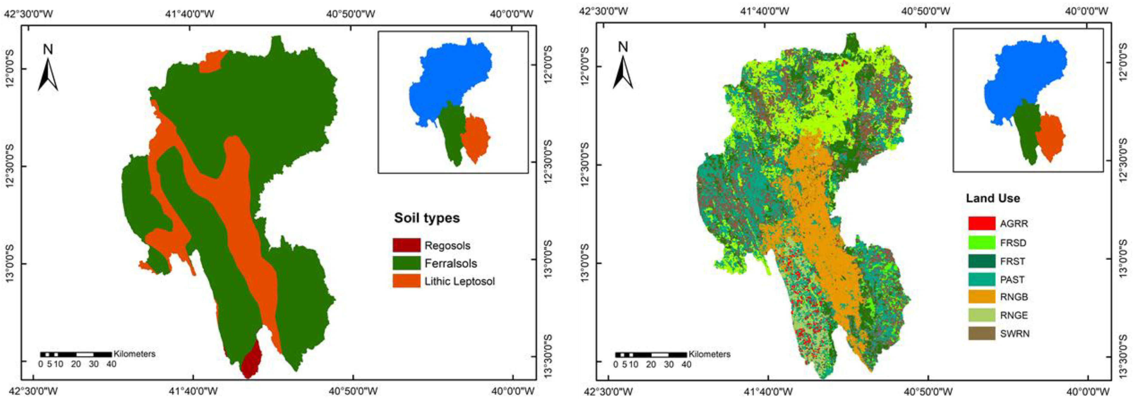
Water 10 01137 g001
Figure 2. Soil and Land use maps of the High Paraguaçu region.
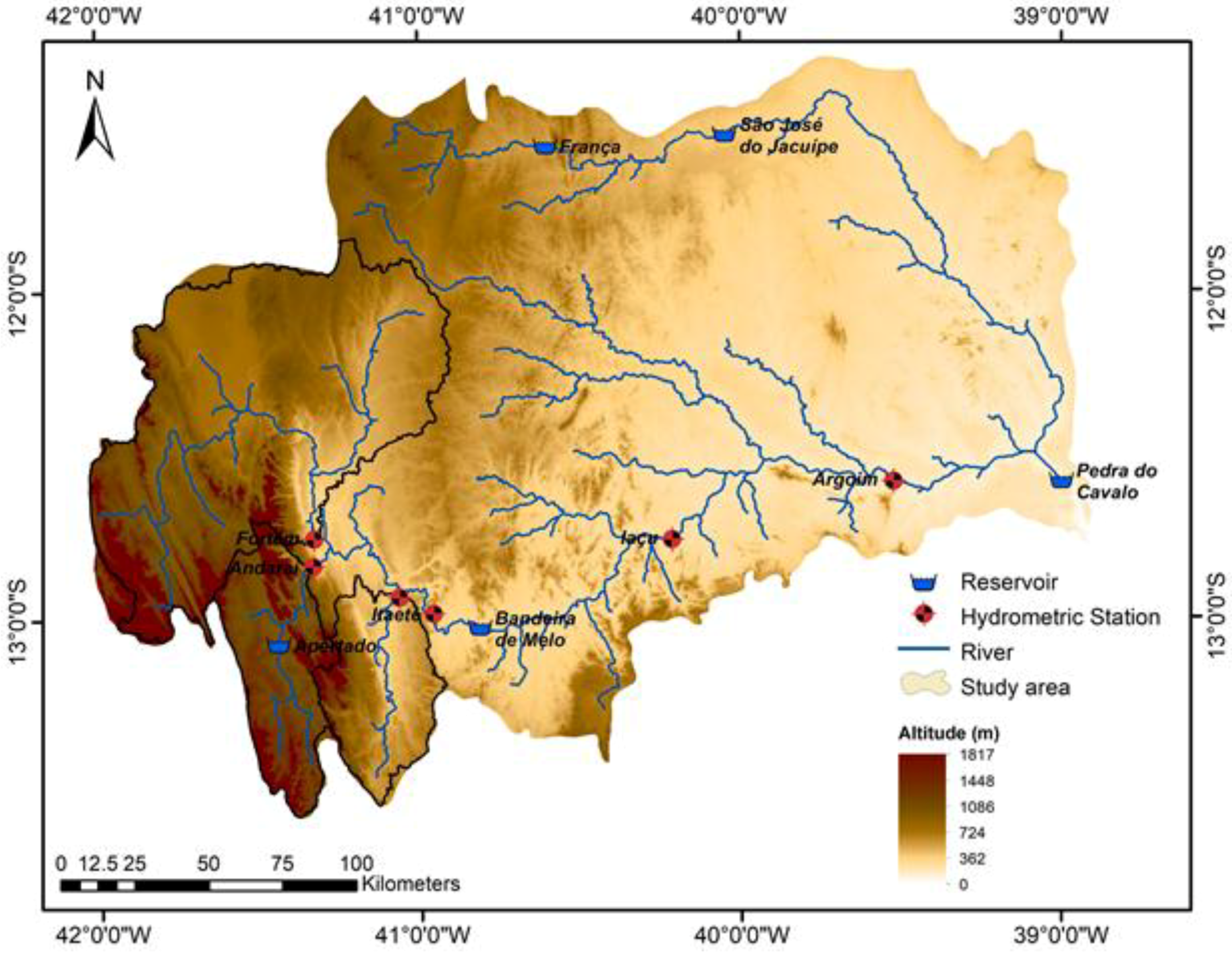
Water 10 01137 g002
Figure 3. Digital elevation model of the Paraguaçu watershed. Location of reservoirs and hydrometric stations.
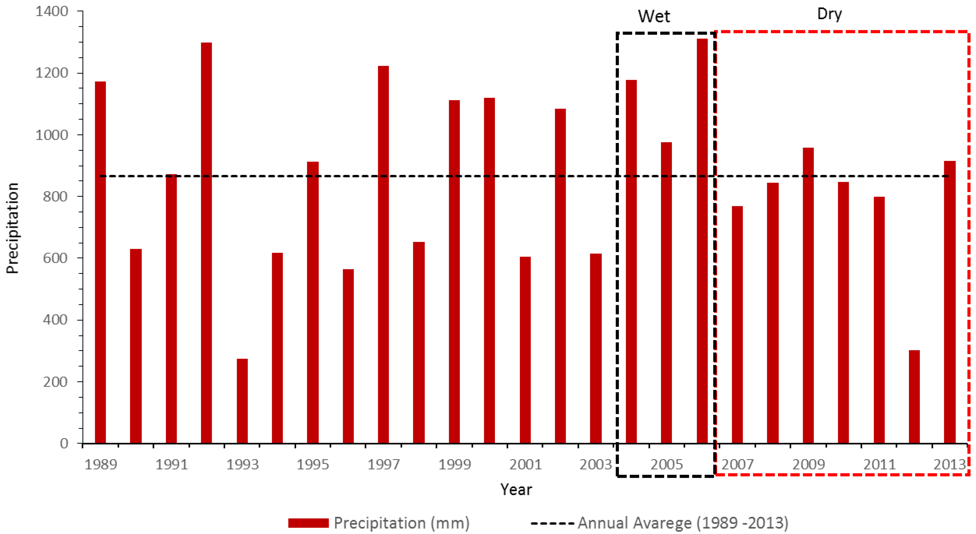
Water 10 01137 g003
Figure 4. Annual precipitation values for the Andarai sub-basin during 1989–2013. Wet and Dry periods chosen for the differential split-sample test.
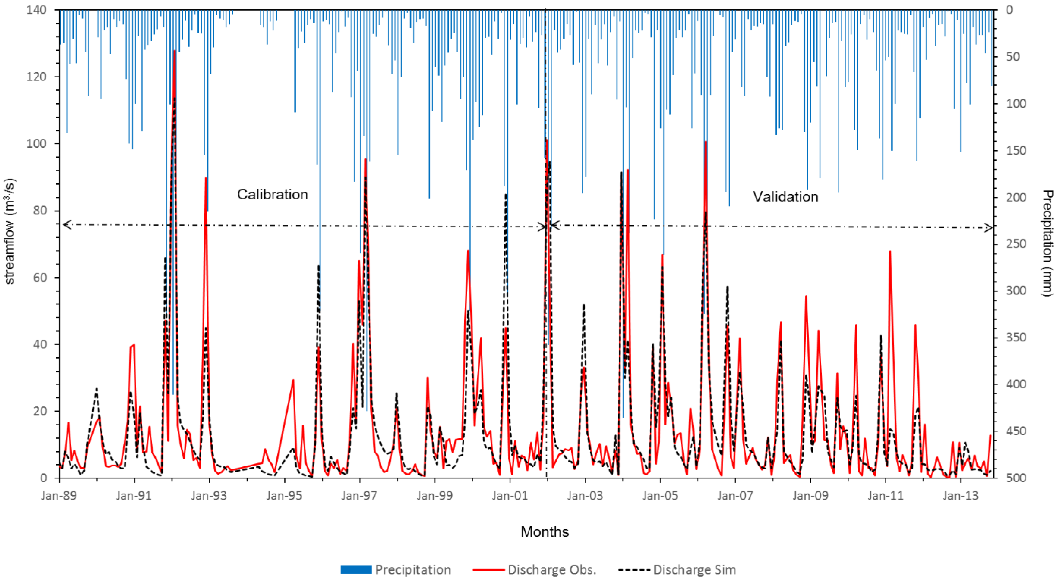
Water 10 01137 g004
Figure 5. Monthly simulated and observed streamflow values in the Andaraí sub-basin (calibration: 1989–2001; validation: 2002–2013).
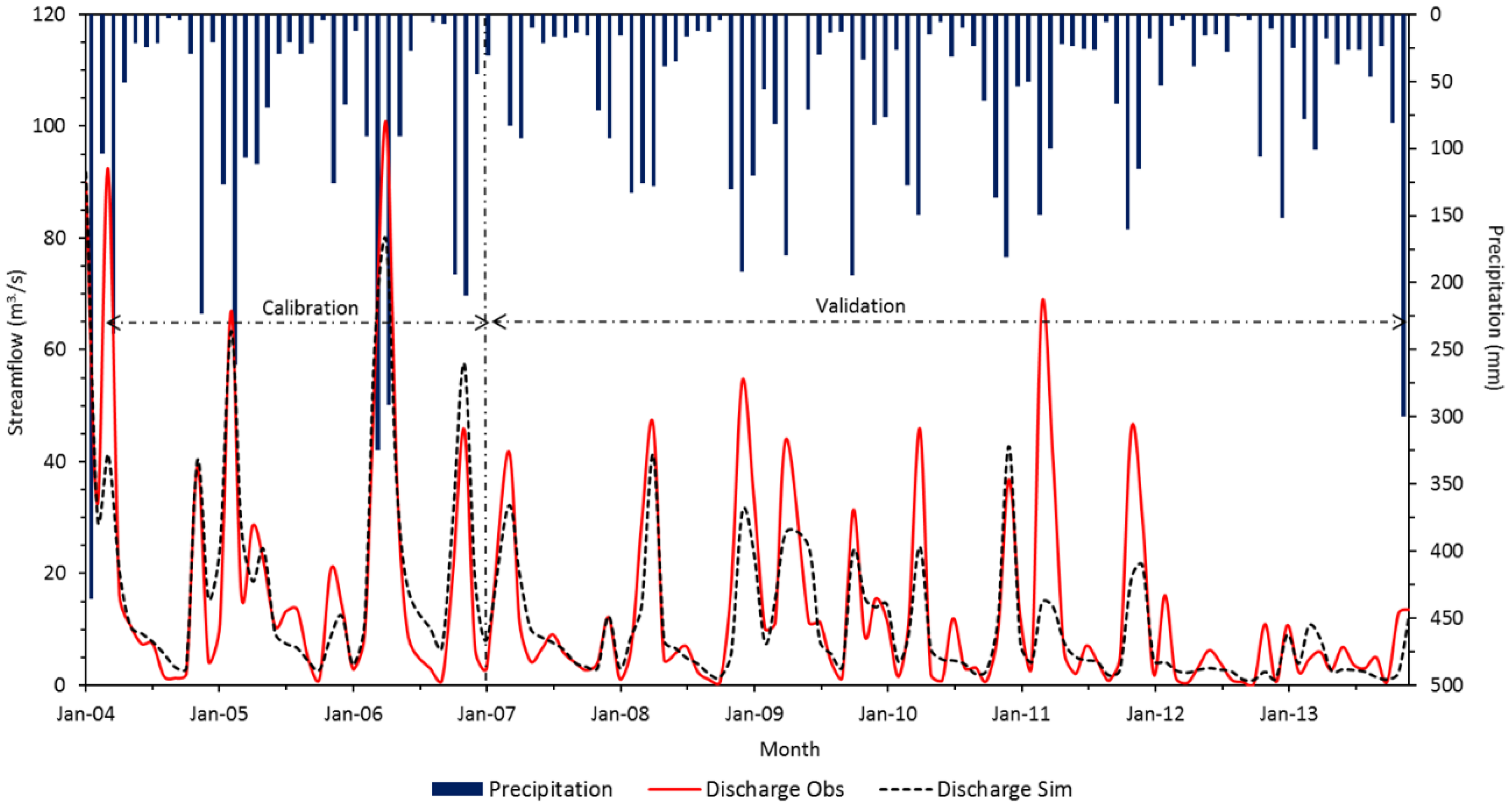
Water 10 01137 g005
Figure 6. Monthly simulated and observed streamflow values in the Andaraí sub-basin (calibration: 2004–2006; validation: 2007–2013).
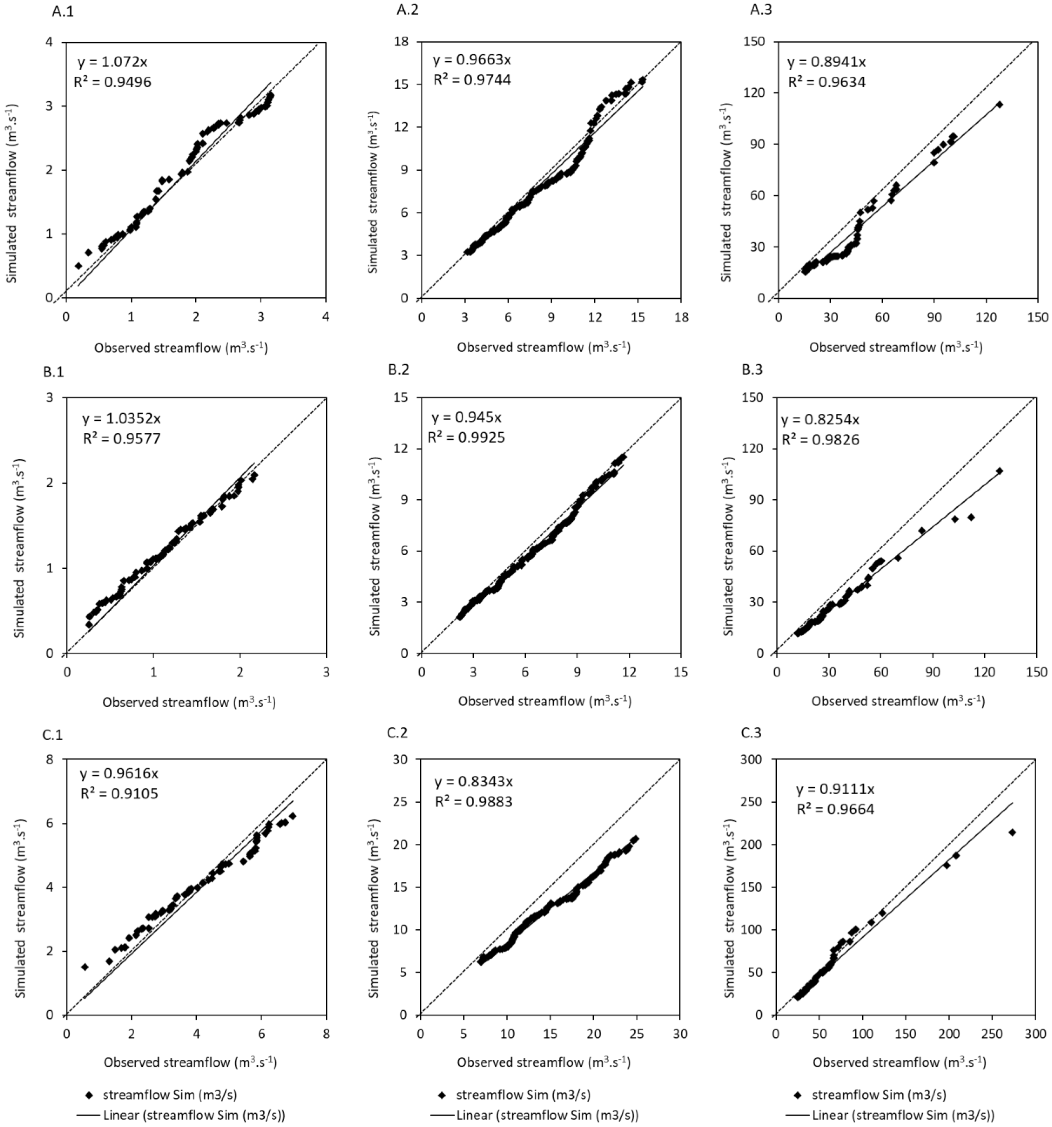
Water 10 01137 g006
Figure 7. Regression analysis between monthly simulated and observed streamflow among 1989–2013 separated for quartile (1—first, 2—second and 3—third quartiles). Sub-basins: Andaraí (A), Iguaçu (B) and Fortém (C).
Water 10 01137 g007
Figure 8. Observed and simulation monthly flow curves in Andaraí (a), Iguaçu (b) and Fortém (c) sub-basins.
Water 10 01137 g008
Table 1. Land use in the Andaraí, Iguaçu and Fortém sub-basins.
BasinAREA (km2)PAST (%)SWRN (%)FRST (%)FRSD (%)RNGE (%)RNGB (%)AGRR (%)
Andaraí2313.8024.583.964.593.2622.1434.646.82
Iguaçu2034.0326.5015.6322.5810.4824.400.240.17
Fortém9426.5025.8122.9812.8727.620.3410.110.27
PAST, pasture; SWRN, caatinga; FRST, mixed forest; FRSD, deciduous forest; RNGE, cerrado, RNGB, bushes cerrado; AGRR, agricultural land.
Table 2. Location of pluviometric and weather stations and sensors used for monitoring weather variables.
StationCode EntityCoordinatesAltitude (m)Sensors
Latitude (°)Longitude (°)
Andaraí *1241008ANA−12.80−41.33330raingauge (0.1 mm)
Usina Mucugê *1241033ANA−13.01−41.37870raingauge (0.1 mm)
Lençóis **83242INMET−12.57−41.38439***
Faz-Ribeiro *1241027ANA−12.06−41.12450raingauge (0.1 mm)
Utinga *1241028ANA−12.50−41.21357raingauge (0.1 mm)
* Pluviometric station; ** Meteorological station; *** sensors can be assessed at http://www.inmet.gov.br/portal/index.php?r=home/page&page=instrumentos.
Table 3. Location of the hydrometric station and sensors used for monitoring river discharge.
StationCodeCoordinatesSensors
Latitude (°)Longitude (°)
Andaraí51120000−12.84−41.33Pressure transducers (1 cm)
Iguaçu51230000−12.93−41.06Pressure transducers (1 cm)
Fortém51190000−12.76−41.33Pressure transducers (1 cm)
Table 4. Default and calibrated parameters used in model simulations.
ParameterDescriptionDefaultCalibrated Value
GW_DELAYGroundwater Delay (days)0–50031–365
GW_REVAPRevaporation coefficient (-)0.02–0.20.02–0.2
GW_RCHRG_DPDeep aquifer recharge (mm)0–10.05–0.25
Mgt1_CN2SCS runoff curve number for moisture condition II (-)35–8945–78
HRU_SLSOILHillslope length (m)0–1500–85
SOL_AWCAvailable water capacity of the soil layer (mm/mm soil)0.075–0.400.1–0.30
SOL_ZSoil depth (mm)-500–3000
SOL_KSaturated hydraulic conductivity (mm/h)-2–35
CH_K2hydraulic conductivity of channel (mm/h)0.01–5000.01–1.5
Table 5. Goodness-of-fit indicators obtained after comparison of model simulations and measured values in the Andaraí sub-basin based on the split-sample test (NSE, model efficiency; PBIAS, percent bias; R2, coefficient of determination).
SeasonDischarge Average (m3/s)Statistic DailyStatistic Monthly
ObservedSimulatedNSERSRPBIASR2NSERSRPBIASR2
1989–201315.1113.880.450.748.20.530.790.456.300.79
1989–200114.5913.050.490.7110.40.540.820.429.860.82
2002–201315.6214.720.420.766.00.520.760.493.410.76
Table 6. Goodness-of-fit indicators obtained after comparison of model simulations and measured values in the Andaraí sub-basin based on the differential split-sample test (NSE, model efficiency; PBIAS, percent bias; R2, coefficient of determination).
PeriodsDischarge Average (m3/s)Statistic DailyStatistic Monthly
ObservedSimulatedNSERSRPBIASR2NSERSRPBIASR2
Wet (2004–2006)23.2223.910.470.80−3.00.600.830.43−1.930.83
Dry (2007–2013)12.7710.200.500.7020.20.510.630.6116.50.66
Table 7. Goodness-of-fit indicators obtained after comparison of model simulations and measured values in the Iguaçu and Fortém sub-basins (validation period 2002–2013) based on the proxy-catchment test (NSE, model efficiency; PBIAS, percent bias; R2, coefficient of determination).
LocationDischarge Average (m3/s)Statistic DailyStatistic Monthly
ObservedSimulatedNSERSRPBIASR2NSERSRPBIASR2
Andaraí (calibration)14.5913.050.490.7210.40.540.820.459.860.82
Iguaçu (validation)11.259.900.440.7312.00.450.750.509.10.76
Fortém (validation)19.8917.880.360.8210.00.450.800.448.60.83
Table 8. Goodness-of-fit indicators obtained after comparison of model simulations and measured values in the Andaraí, Iguaçu and Fortém sub-basins based on the proxy-catchment differential split-sample test (NSE, model efficiency; PBIAS, percent bias; R2, coefficient of determination).
PeriodsDischarge Average (m3/s)Statistic DailyStatistic Monthly
ObservedSimulatedNSERSRPBIASR2NSERSRPBIASR2
Andaraí—Wet 23.2223.910.470.80−3.00.600.830.41−1.930.83
Iguaçu—Dry8.606.330.360.8026.00.390.500.7021.00.54
Iguaçu—Wet18.0816.860.470.726.70.480.800.468.100.83
Andaraí—Dry12.7710.200.500.7020.20.510.630.6116.50.66
Table 9. Soil water balance in Andaraí, Iguaçu and Fortém.
Total Amount (mm)Fraction of Precipitation (%)
AndaraíIguaçuFortémAndaraíIguaçuFortém
Precipitation866.5701.2784.3---
Evapotranspiration599.8541.4675.069.277.286.1
Runoff96.738.728.511.25.53.6
Lateral flow76.552.837.88.87.54.8
Base flow48.040.720.65.55.82.6
Soil storage45.527.622.45.33.92.9
Table 10. Minimum and actual annual actual evapotranspiration values in Andaraí, Iguaçu and Fortém per land use.
BasinRangePASTSWRNFRSTFRSDRNGERNGBAGRR
Annual Actual Evapotranspiration (mm)
AndaraíMinimum324312255284314278562
Maximum104072312221227725719810
IguaçuMinimum200210143177182191537
Maximum99164610441042644643727
FortémMinimum252303228243301278253
Maximum129411121411142011077741097
PAST, pasture; SWRN, caatinga; FRST, mixed forest; FRSD, deciduous forest; RNGE, cerrado, RNGB, bushes cerrado; AGRR, agricultural land.
Table 11. Results of the regression analysis and paired t-test on observed and simulated average monthly (1989–2013).
Fluviometric StationQuartilenatcaltcritR2
Andaraí710.891.14(ns)1.9770.96
2º and 3º1400.970.79(ns)1.9680.97
701.07−1.37(ns)1.9770.95
Iguaçu740.821.42(ns)1.9760.98
2º and 3º1480.951.13(ns)1.9780.99
741.04−0.94(ns)1.9760.96
Fortém680.910.59(ns)1.9780.97
2º and 3º1330.834.16 *1.9690.99
670.960.12(ns)1.9780.91
n—number of sample value; a—regression coefficient; tcal —paired t-test, calculated value; tcrit—paired t-test, two-tailed value; ns—not significant at 5% level of significance; * significant at the 5% level of significance.
Table 12. Comparison exceedance Q90 and Q95 values between observed and simulated monthly flow for the period to 1989–2013.
Station90% Exceedance95% Exceedance
QobsQsimError (%)QobsQsimError (%)
Andaraí1.471.8324.00.981.08.0
Fortém3.383.668.02.633.016.0
Iguaçu0.971.0710.00.610.7014.0

