Article

An Efficient Numerical Model to Predict the Mechanical Response of a Railway Track in the Low-Frequency Range

1
Université Paris-Saclay, CentraleSupélec, ENS Paris-Saclay, CNRS, LMPS—Laboratoire de Mécanique Paris-Saclay, 91190 Gif-sur-Yvette, France
2
SNCF Réseau, 6 Avenue François Mitterrand, 93574 La Plaine Saint-Denis, France
*
Author to whom correspondence should be addressed.
Vibration 2022, 5(2), 326-343; https://doi.org/10.3390/vibration5020019
Submission received: 6 April 2022 / Revised: 13 May 2022 / Accepted: 20 May 2022 / Published: 24 May 2022
(This article belongs to the Topic Dynamical Systems: Theory and Applications)

Abstract

:
With railway interoperability, new trains are allowed to move on the French railway network. These trains may present different designs from standard trains. This work aims to complete the current approach for vehicle admission on the railway network, which is defined in technical baselines. Historically, computation rules for traffic conditions are based on simplified analytical works, which are considerably qualitative. They have evolved through feedback and experimental campaigns to comply with the track structure evolution. An efficient methodology based on numerical simulation is needed to evaluate railway vehicle admission to answer this issue. A perspective to update these computation rules is to evaluate the structural fatigue in the rail. That is to say, fatigue is caused by bending and shear stresses. The complexity of the railway system has led to an investigation at first of the vertical response of the railway track and quantifying its contribution to the rail’s stress response. In that sense, this paper investigates the vertical track response to a moving railway vehicle at low frequencies. For this purpose, a lightweight numerical model for the track, a multi-body model for the vehicle, and a random vertical track irregularity are proposed. More explicitly, the track model consists of a two-layer discrete support model in which the rail is considered as a beam and sleepers are point masses. The rail pads and ballast layer are modelled as spring/damper couples. Numerical results show a negligible effect of track inertia forces due to high track stiffness and damping. Nevertheless, this assumption is valid for normal rail stresses but not for ballast loading, especially in the case of sleeper voids or unsupported sleepers. Hence, the prediction of the mechanical stress state in the rail for fatigue issues is achieved through a static track model where the equivalent loading is obtained from a dynamic study of a simplified vehicle model. A statistical analysis shows that the variability of the vertical track irregularity does not influence the output variabilities like the maximum in time and space of the normal and shear stress.

1. Introduction

Currently, the procedure for railway vehicle admission on a track of the French railway network is presented in a technical baseline. It is defined for conventional railway lines, which are highly heterogeneous in terms of mechanical resistance. The procedure consists of verifying the compatibility between the vehicle and the track regarding:
  • the type of vehicle and its static wheel loads,
  • the mechanical resistance of the track and its layout [1].
Then, for each combination of the track and the vehicle, the maximum allowed speed of the vehicle V max is identified. Conventional lines are limited to a maximum speed of 220 km/h. When coupled to track geometry irregularities (i.e., minimum wavelength of 3 m), a relevant frequency range of [0;20 Hz] is defined. This frequency range is also the scope of security and passenger comfort matters [2], which concerns the railway vehicle admission procedure. The current computation rules behind railway vehicle admission are derived from simplified analytical works aiming to classify the network’s tracks with respect to their flexural resistance [3]. These rules have evolved through feedback. However, with the strengthening of the railway interoperability strategy, new trains with different designs are allowed to move on the French railway network. Thus, the main objective of this work is to complete the current approach to cover new trains and potentially new track designs. Furthermore, increasing traffic density and enhancing the railway network’s exploitation performances requires improvement of the current railway vehicle admission rules. Finally, to ensure optimal network exploitation, it is necessary to provide quick decisions for railway vehicle admission. The main objective of this work is to propose an efficient methodology that supports the railway vehicle admission procedure and allows for the definition of new rules for traffic conditions based on the evaluation of fatigue in the rail. The proposed approach is based on numerical modelling of the railway track and the vehicle to combine accuracy and speed.
In this context, several numerical models of the track have been developed in the literature. 3D finite element (FE) models allow for a better representation of the track components and their constitutive laws, sometimes taking into account high speed configurations ([4,5,6]). For instance, Mei et al. [7] studied the impact of vertical track defects and moving railway heavy hauls on the dynamic stress at the subgrade surface modelled as a Mohr–Coulomb constitutive law. Varandas et al. [8] focused on the estimation of the ballast and sub-ballast long-term deformation through a 3D model where the ballast layer is assimilated to a non-linear material law. Sayeed and Shahin [9] investigated the critical speed of the railway track where ballast and interface layers were modelled as elastoplastic Mohr–Coulomb materials. Although accurate, 3D models remain hardly suitable for industrial exploitations because of the large computational time. Hence, reduced models have been proposed [10,11] where the analysis of the overall domain is restricted to a reference cell by taking advantage of the track periodicity. Then, reduction techniques are adopted to reduce the number of degrees of freedom of the system (DOFs). In that case, non-periodic track irregularities cannot be implemented. Other authors proposed 2D models with a plane stress formulation [12] or a plane strain formulation [13]. These models give a good approximation of the stress in the section of the track, but realistically, the stress response is heterogeneous with respect to the track width. All these models are useful when an accurate characterisation of the subgrade or ballast layer is required. Beam-like structured finite element models of the track are more convenient to study the response of the track upper structure {rail, sleeper} than moving vehicles which are represented by linear multi-body models. This model category is suitable for industrial exploitations in terms of the computational costs and effectively predicts the track dynamic response. For example, the computed vertical receptance curve in the work of Xie and Iwnicki [14] indicates resonance occurring in the high-frequency domain for a beam-like track model with two layers and discrete supports. It is essential to supply the vehicle and track models with correct values of damping and rigidity to gain representative results. This category of track models was used to study the dynamic effects of vehicles moving on periodic defects such as corrugated rails [14,15,16] or wheelflats [17], or non-periodic defects, including welded joint defects [18] and unsupported sleepers due to degradation of the ballast [15]. The effect of long-wavelength track geometry irregularities was also investigated in [19,20,21], where random track irregularities are generated from single-sided power spectral density functions. This category of track models is still relevant. For instance, the vertical dynamic response of a ballasted track under a moving multi-body vehicle model was studied in [22]. More specifically, a sensitivity analysis on axle loads showed a linear increase in the contact forces and transmitted forces of the track with axle loads. The train running security and passenger comfort were studied in [23] through the analysis of wheel–rail forces in a track–bridge model. In [24], the vertical interaction between a track and a bridge was investigated. Moreover, the influence of dynamic train loads and temperature variations in the damage state of a tram ballastless track was studied in [25]. In [26], the mechanical response of the different substructure layers was evaluated using a rheological model of the track substructure, including plasticity (i.e., slider elements). Furthermore, a 2D two-layer model of the track was used in [27] to analyse the critical velocity of the track and the instability of moving masses.
This paper is an intermediate step to answering the main objective. A beam-like structure finite element model of the track is developed to investigate the bending and shear stress response of the railway track and to quantify its contribution to the rail’s stress response. The objective is to predict the stress state in the rail when the track is subjected to the dynamic loading of a vehicle modelled as a multi-body system running on a track with irregularities. Indeed, the idea is to quickly provide relevant information on the capacity of the railway to bear the vehicle load.
The first section is dedicated to the description of the railway system model. It includes the finite element model of the track, the methodology used to generate random vertical track irregularities from existing measurements and a multi-body model of the railway vehicle. Then, numerical applications are presented to study the effect of track inertia forces on the mechanical stress response of the rail. The stress state in the rail is also analysed to verify the possible predominance (or not) of the normal stress over the shear stress. In the last section, a statistical analysis based on the Monte Carlo simulation is available to identify the effect of the track irregularity variability on the rail’s stress response.

2. Materials and Methods

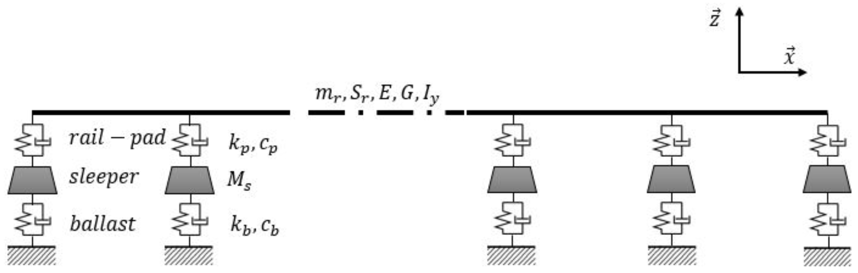
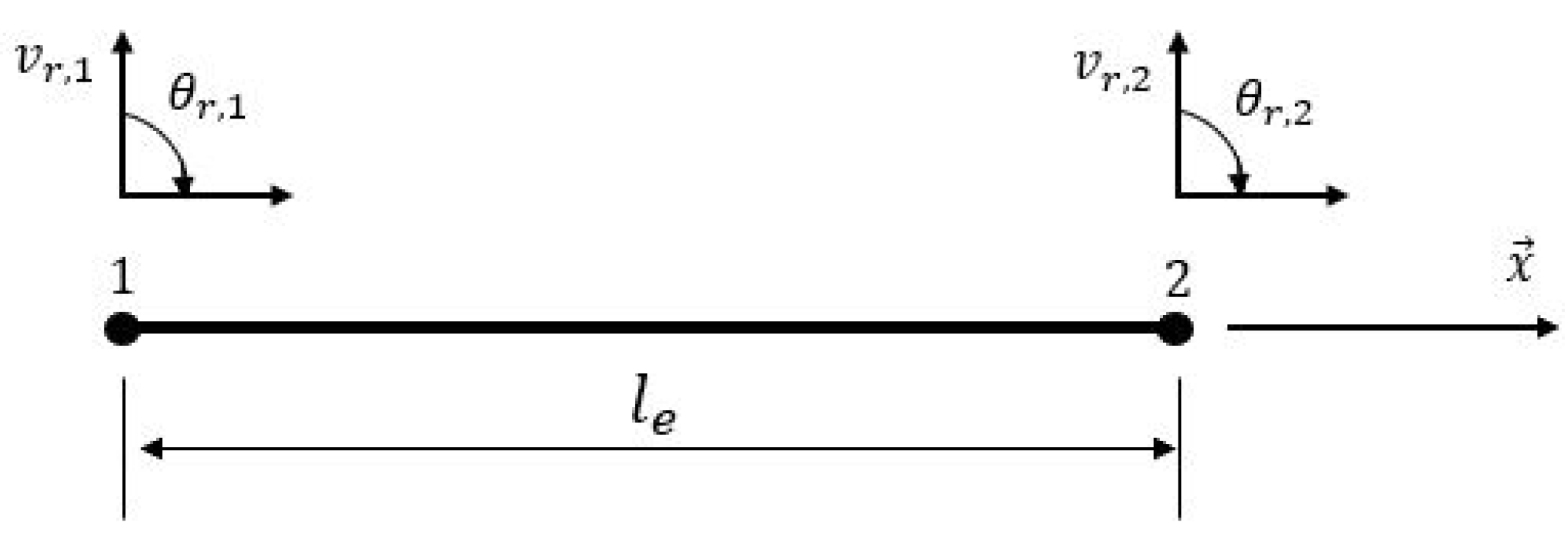
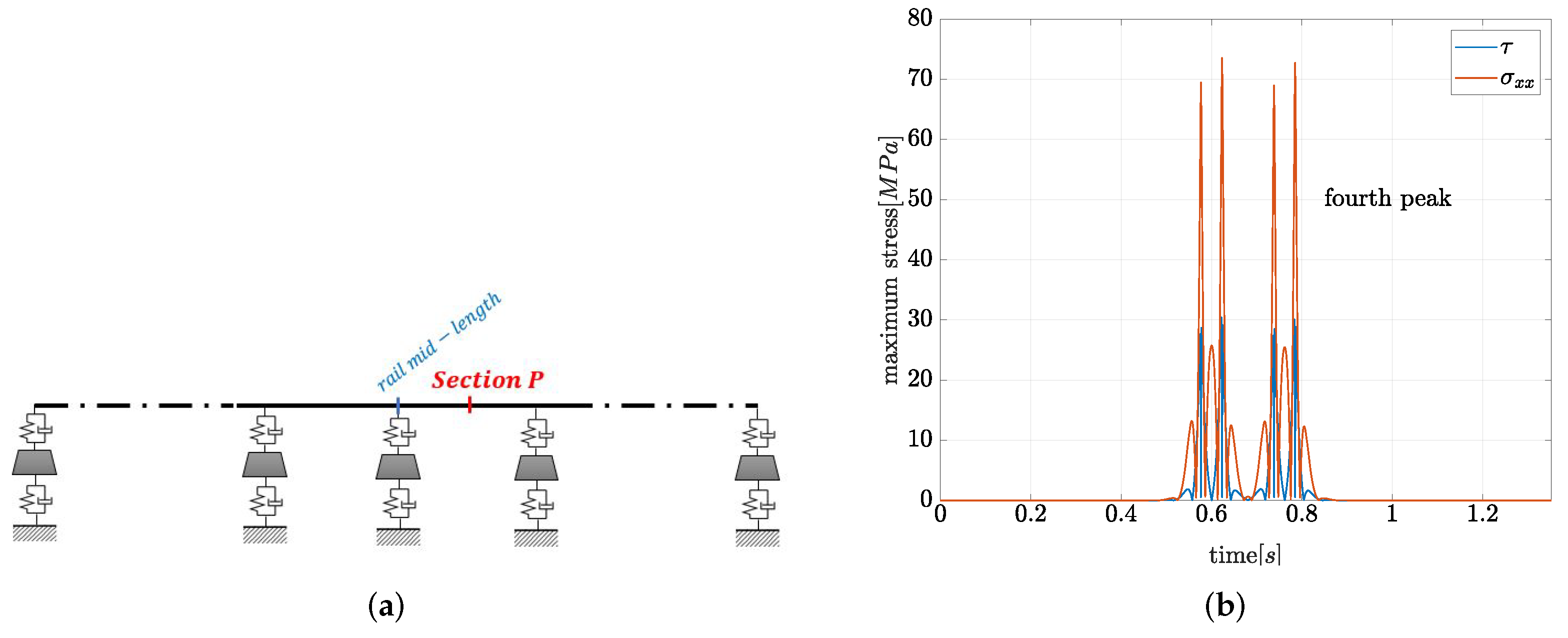
2.1. Finite Element Model of the Track

A lightweight finite element model of the track is developed. In the present work, regarding the symmetry of the track in its longitudinal direction, only half of the track is modelled (i.e., one rail). It describes a discretely supported rail on rail-pads and sleepers laying on a ballast layer as shown in Figure 1.
In particular, considering the negligible longitudinal displacement, the rail is discretised as two-node Timoshenko beam elements with two degrees of freedom each: a vertical displacement v r , i and a rotation θ r , i (Figure 2). The rail is also characterised by its specific mass m r , shear and Young modulus G and E, cross-section S r and moment of inertia I y concerning the y axis. The sleepers have only a vertical displacement v s , j . The sleepers are assumed to be rigid, and their inertia is neglected. Thus, in the dynamic calculation, they are only represented by point masses. They are linked to some rail nodes by parallel spring/damper couples representing the rail-pad behaviour between a sleeper and the rail. The ballast layer is also represented by parallel spring/damper couples.
Stiffness coefficients of the spring for rail-pads and the ballast are, respectively, k p , k b and damping coefficients are, respectively, c p , c b . The finite element method to compute degrees of freedom in the rail is recalled in Appendix A.

2.2. Track Loading

The vertical track response is studied in the low-frequency range [0;20 Hz] as it concerns railway vehicle admission on conventional lines, which deals with security and passenger comfort matters. It allows for uncoupling of the vehicle’s dynamic from the track’s dynamic. Indeed, according to [28,29,30], at a low-frequency range, track inertia forces are negligible compared to vehicle’s inertia and do not impact the vehicle’s dynamic behaviour. On the one hand, receptance measurements of the track show that the natural frequencies are much higher than the frequency range of interest ([0;20 Hz]). Indeed, a first resonance is in the frequency range [50;30 Hz], a second one is in the frequency range [200;600 Hz], and a third one is located around 1000 Hz as explained in [31]. On the other hand, natural vibrations of the vehicle motion are in the area of [0;20 Hz] [30,32]. Therefore, the vertical track loading is due to:
  • the static wheel loads of the vehicle,
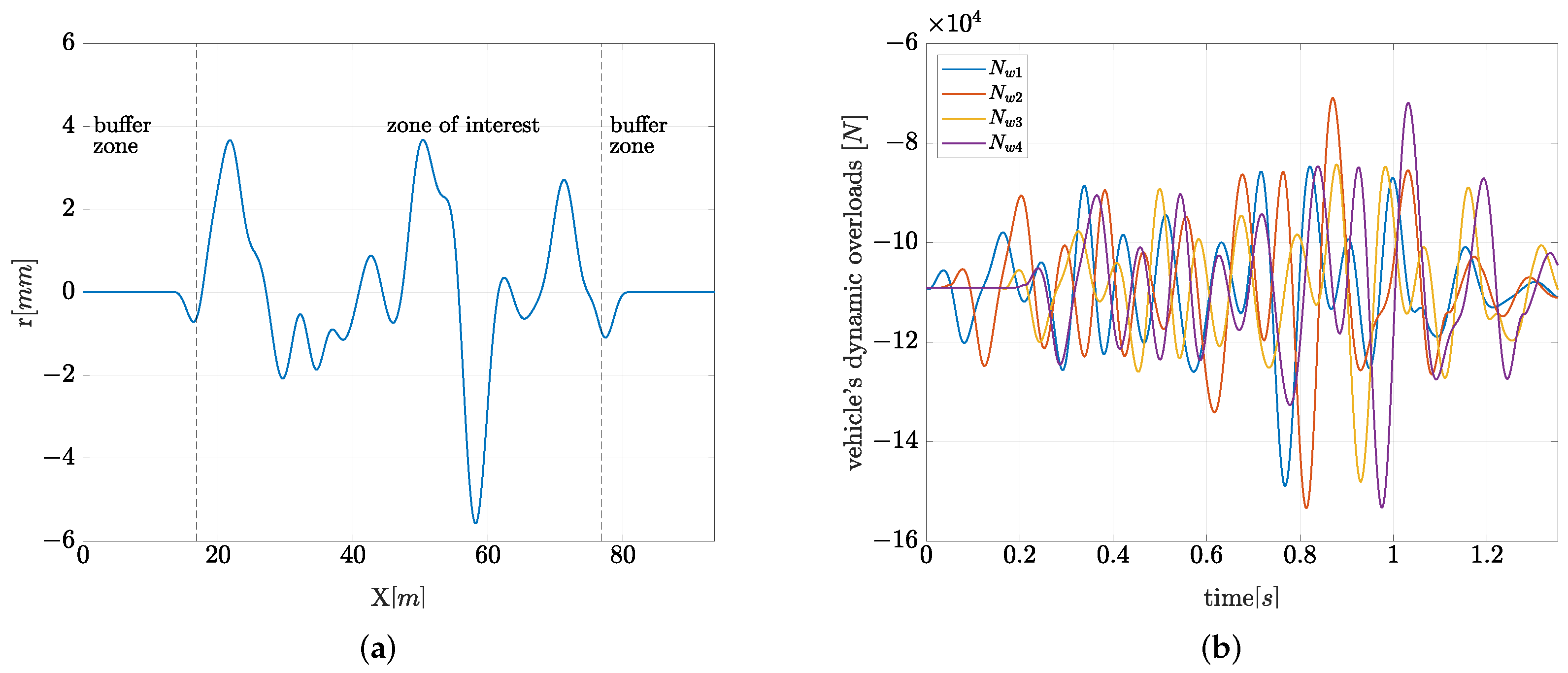
  • the vehicle’s dynamic overloads due to irregularities of the track vertical profile.

2.2.1. Simulation of a Random Irregularity of the Track Vertical Profile

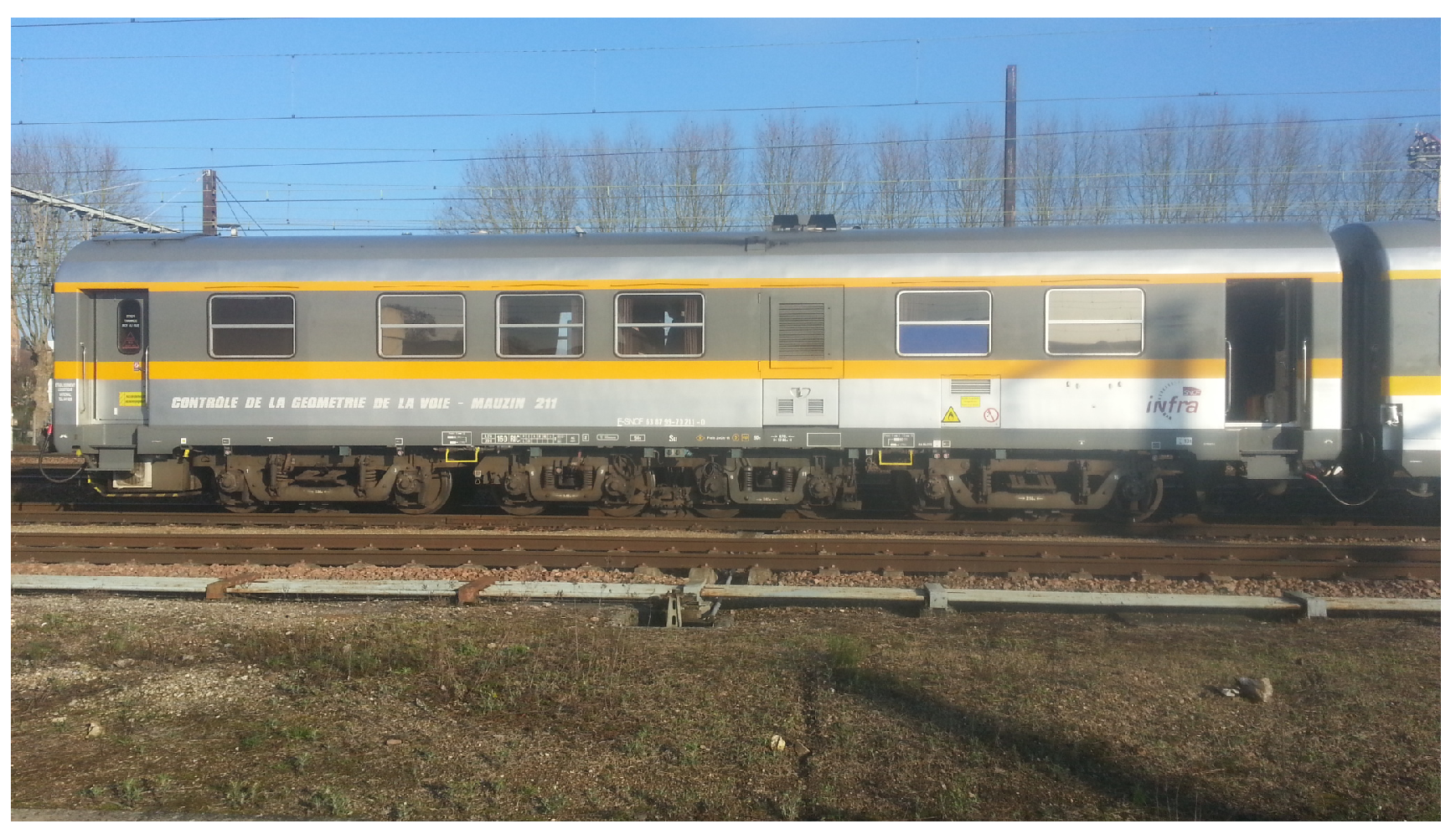
Track Inspection Techniques in the French Railway Network

For French conventional railway lines where speeds are limited to 220 km/h, track inspections are achieved by Mauzin cars (Figure 3). The vehicle includes 3 bogies, 8 wheelsets and an extremely rigid car body that constitutes the reference plane for track geometry measurements.
Several geometry irregularities are recorded (gauge, alignment, cross-level and vertical profile). Given the purpose of studying the vertical track response, only the vertical profile irregularity is introduced. The vertical profile of the track is measured by the variations between the vertical displacement of a wheel of the Mauzin car and the average of the vertical displacements of all the corresponding wheels [33]. Besides this geometrical measurement, track experts in France use a quality indicator for the track according to which maintenance operations are planned. In more detail, for the vertical profile, the longitudinal levelling (NL) is used. It is the standard deviation of the measured vertical profile for a distance of 200 m [12].

Methodology for Generating the Random Irregularity of Track Vertical Profile

Many authors proposed a theoretical modelling of the random irregularity for the track vertical profile [7,19,20,21,34,35]. Ref. [20] considered the vertical track profile irregularity as a stationary ergodic Gaussian random process that can be defined by a power spectral density (PSD) and a zero expectation. The defect sample is then recovered by inverse Fourier transform. This theoretical approach is simple to implement and gives a first estimation of geometrical irregularities. However, generated track irregularities are not well representative of real measurements in the French railway network. Generating the vertical track irregularity from the PSD requires that the track is free from turnouts or road crossing and that the railway line is free of track deterioration (e.g., ballast layer deterioration) [20], which is not always possible to satisfy, particularly when a local change in the track substructure is required. Besides, because of the interaction between the vehicle and the track, track irregularities are, in reality, neither Gaussian nor stationary, according to Perrin et al. [36].
A new approach is conducted in this paper to generate a random vertical track irregularity r ( x ) from vertical defect measurements r mes ( x ) on different zones in alignment of a given track. This allows us to create a sample representative of the measured track zones and characterised by the richest frequency content in terms of frequency bandwidth and magnitude response. It consists of the following steps:
  • A first preprocessing on the vertical measurements r mes ( x ) is achieved by removing track zones which are in curves since the modelled track is fully in alignment. N s is thus the total number of track zones in alignment.
  • For each track zone, a discrete Fourier transfom (DFT) of the measured signal r mes ( x ) is performed with zero padding, where N is the size of the longest signal, f n is the frequency and i is the imaginary number:
    H mes ( f n ) = k = 0 N 1 r mes ( x ( k ) ) e 2 π i N k n for 0 n N 1
  • At each spectral component f n between 0 and the Nyquist frequency (i.e., 0 n N 2 ), the maximum amplitude of the DFT H mes among the N s signals is extracted:
    | H ( f n ) | = max 1 α N s | H mes ( f n ) | α
  • By creating uniformly distributed random phases ϕ n = ϕ ( f n ) in [0; 2 π ] at each spectral component, one can construct the positive frequency domain signal:
    H ( f n ) = | H ( f n ) | e i ϕ n for 0 n N 2
    The negative frequency domain signal is calculated as the complex conjugate of the positive frequency domain signal. Hence, the DFT H of the random vertical track irregularity r ( x ) is built,
  • The track vertical irregularity r ( x ) is recovered by inverse fourier transform:
    r ( x ( n ) ) = 1 N k = 0 N 1 H ( f k ) e 2 π i N k n for 0 n N 1

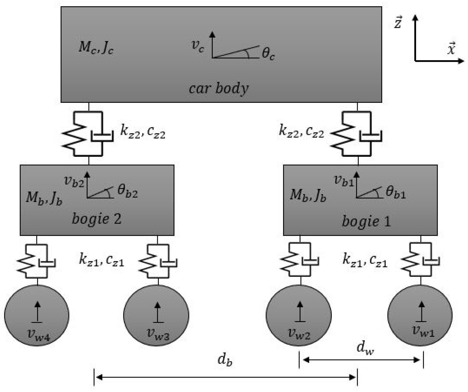
2.2.2. Multi-Body Model of the Railway Vehicle

A model of a half-locomotive is proposed in Figure 4 due to the ( x , z ) symmetry plane of the vehicle.
It consists of a multi-body system where the car body is defined by a vertical motion v c and a rolling motion θ c . Each bogie has a vertical motion v b i and a rolling motion θ b i . As mentioned in Section 2.2, the track’s vibration is supposed negligible in front of the irregularity amplitude. Thus, the vehicle is expected to follow the track irregularity profile and the vertical displacements of the wheels v w i can instantly be written as a function of the vertical irregularity profile r:
v w 1 = r ( V t ) v w 2 = r ( V t d w ) v w 3 = r ( V t d b ) v w 4 = r ( V t ( d w + d b ) )
where V is the speed of the vehicle, which is supposed to be constant, d w is the wheelbase and d b is the distance between the two bogie centrelines. The equations of motion of the vehicle system are solved with a static equilibrium as the initial condition:
[ M v ] { v ¨ } + [ C v ] { v ˙ } + [ K v ] { v } = { F } { v ( t = 0 ) } = [ K v ] 1 { F } { v ˙ ( t = 0 ) } = 0
The nodal displacement vector { v } and the force vector { F } are expressed by:
{ v } = v c θ c v b 1 θ b 1 v b 2 θ b 2 T { F } = M c g 0 M b g + c z 1 v ˙ w 1 + v ˙ w 2 + k z 1 v w 1 + v w 2 c z 1 d w 2 v ˙ w 1 v ˙ w 2 k z 1 d w 2 v w 1 v w 2 M b g + c z 1 v ˙ w 3 + v ˙ w 4 + k z 1 v w 3 + v w 4 c z 1 d w 2 v ˙ w 3 v ˙ w 4 k z 1 d w 2 v w 3 v w 4
The stiffness, damping and mass matrices are formulated as follows:
[ K v ] = 2 k z 2 0 k z 2 0 k z 2 0 0 2 d b 2 2 k z 2 + k θ d b 2 k z 2 k θ d b 2 k z 2 k θ k z 2 d b 2 k z 2 2 k z 1 + k z 2 0 0 0 0 k θ 0 2 d w 2 2 k z 1 + k θ 0 0 k z 2 d b 2 k z 2 0 0 2 k z 1 + k z 2 0 0 k θ 0 0 0 2 d w 2 2 k z 1 + k θ [ C v ] = 2 c z 2 0 c z 2 0 c z 2 0 0 2 d b 2 2 c z 2 + c θ d b 2 c z 2 c θ d b 2 c z 2 c θ c z 2 d b 2 c z 2 2 c z 1 + c z 2 0 0 0 0 c θ 0 2 d w 2 2 c z 1 + c θ 0 0 c z 2 d b 2 c z 2 0 0 2 c z 1 + c z 2 0 0 c θ 0 0 0 2 d w 2 2 c z 1 + c θ [ M v ] = M c 0 0 0 0 0 0 J c 0 0 0 0 0 0 M b 0 0 0 0 0 0 J b 0 0 0 0 0 0 M b 0 0 0 0 0 0 J b
In the above equations, M c is the half car body mass, and J c is the half car body moment of inertia concerning y axis. M b and J b are, respectively, the half bogie mass and the half bogie moment of inertia concerning y axis. k z 1 and c z 1 are, respectively, the vertical stiffness and damping of the primary suspension linking a bogie to a wheel. Finally, k z 2 and c z 2 are, respectively, the vertical stiffness and damping of the secondary suspension linking the car body to a bogie. An angular stiffness k θ and angular damping c θ are added at the level of the secondary suspension as a calibration of the system’s rotational behaviour.
The resolution of the dynamic problem (Equation (6)) and wheels motion equations allow for the calculation of the applied loads on the rail by each wheel of the vehicle. These loads are, in a second step, applied to the track model as the track loading represented by four variable loads, N w 1 ( t ) , N w 2 ( t ) , N w 3 ( t ) and N w 4 ( t ) , moving at a constant speed V.

3. Results

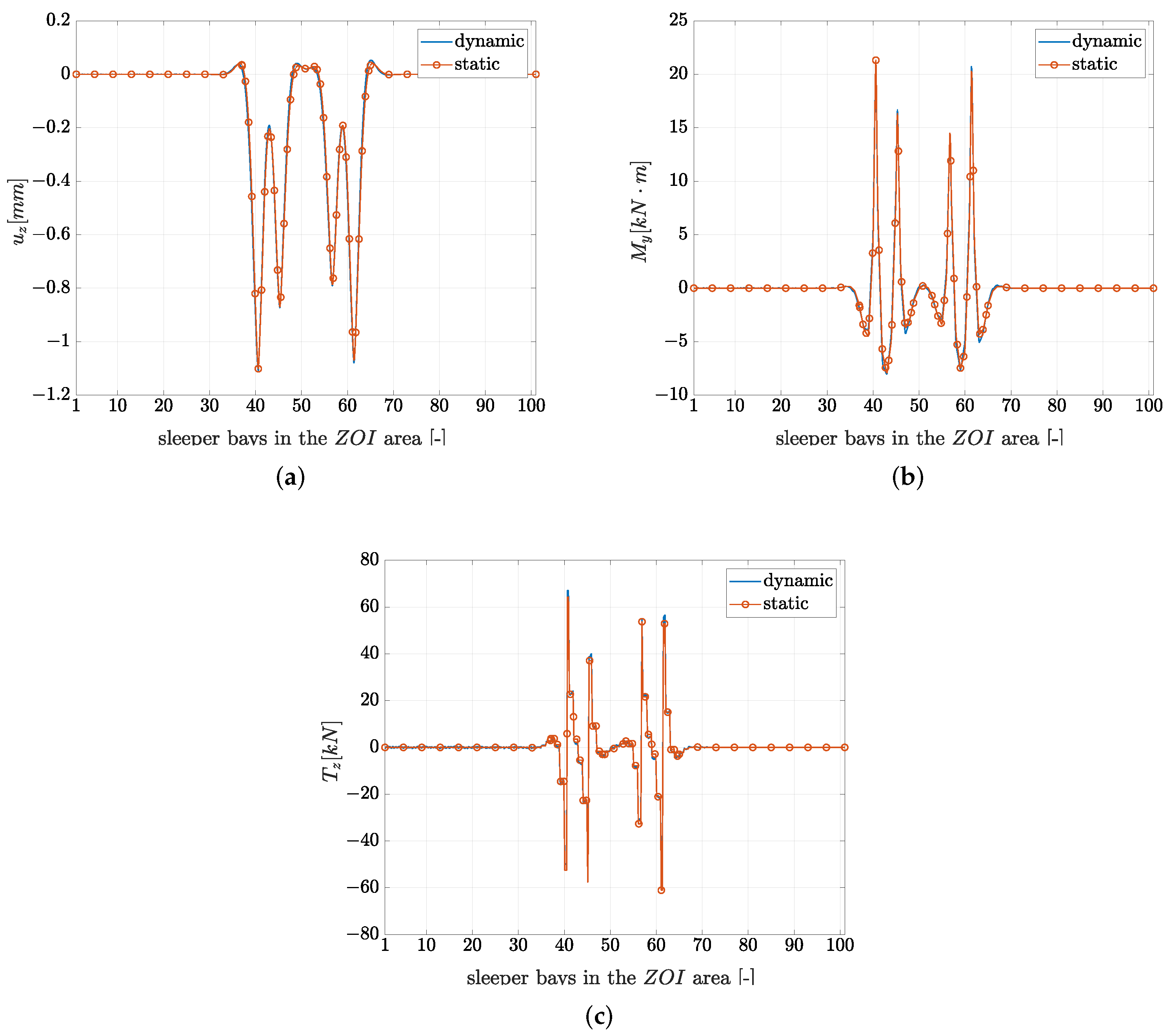
3.1. Vertical Track Response to a Moving Half Vehicle

Parameters of the studied vehicle and track are listed in Table 1. As defined in Section 2.2.1, a vertical track irregularity with wavelengths λ [3;30 m] is generated over a length corresponding to 100 sleeper bays of the track (Figure 5a). Taking into account the fact that only the track’s geometry is supposed to excite the vehicle’s dynamic, calculations are decoupled. For the given vertical track irregularity, the dynamic loads N w 1 ( t ) , N w 2 ( t ) , N w 3 ( t ) and N w 4 ( t ) applied by the vehicle on the track at the level of each wheel are at first computed using the Newmark integration method (average constant acceleration scheme) [37] (Figure 5b). The equivalent loads (at each time step, the position and the amplitude of the force change) are then implemented in the track model developed in Cast3M [38] in order to analyse its response. For the purpose of the study, the vehicle speed V is taken equal to 216 km/h.
The track behaviour is analysed over 100 sleeper bays (i.e., the irregularity’s length). 10 beam elements per sleeper bay are considered, and the time step is chosen so that 3 time steps are necessary for a wheel to move from a node i to a node i + 1 .
The finite length of the track model poses some challenges in efficiently representing the wave propagation problems in railway tracks because of wave reflection at the boundaries. To avoid wave reflection, some authors such as Nguyen [39] added absorbing boundary conditions. Indeed, some elements with high damping are introduced at the boundaries. Another methodology extends the domain significantly so that waves are attenuated before they reach the boundaries. The latter method can be expensive and is appropriate when damping in the structure is essential. For the current track model, a buffer zone without defects is added on both sides of the track (second strategy). The use of the second strategy is motivated by the fact that the modelled track has high vertical damping values. Besides, thanks to the buffer zone, the steady state of the track system is attained when the vehicle reaches the mid-zone area of the track (initial length of the track without the buffer zone), which is known as the zone of interest ZOI. A sensitivity analysis showed that a length equivalent to twice the vehicle’s length with a junction length (i.e., transition from defected to zero defect zone) for the buffer zone was sufficient. The comparison of the dynamic and static response of the track is then conducted.

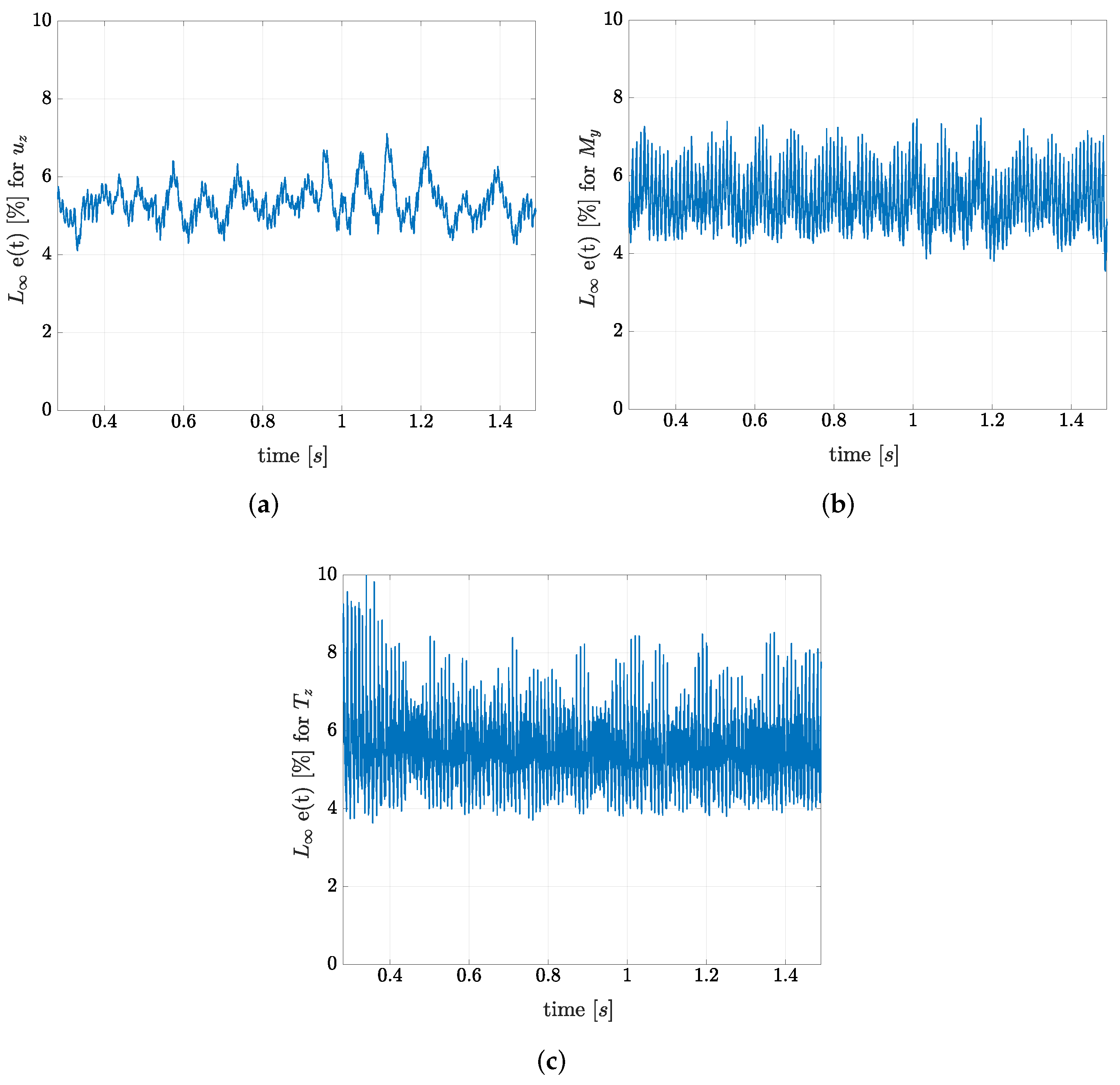
3.1.1. Validation of the Hypothesis of Negligible Inertial Forces at Low Frequency

A comparison of the track dynamic response and its static equivalent response is carried out (Equation (9)). More specifically, the shear force T z , the bending moment M y and the vertical deflection u z in the rail are investigated. Figure 6 shows that the two responses are very close.
[ K ] { u } i = { Q } i
An L norm error is then introduced to quantify the gap between the static response q sta and the dynamic response q dyn in the mid-region of the track between the simulation times t 1 and t 2 corresponding, respectively, to the entry of the first wheel in the ZOI and the exit of the fourth wheel from the ZOI (Equation (10)). As it is reported in Figure 7, the gap does not exceed 10 % .
e ( t ) = max x Z O I | q dyn ( x , t ) q sta ( x , t ) | max x Z O I | q dyn ( x , t ) | for q { T z ; M y ; u z }
The very close responses can be explained by the fact that vertically, the track’s stiffness and damping are very high on one side. On the other hand, the natural frequencies of the track are higher than the range frequency of interest ([0;20 Hz]) [40]. The stress state can thus be computed for a static track response to dynamic vehicle overloads. The buffer zone is consequently reduced to the vehicle’s length so that initially, all vehicle’s wheels are in the plane zone of the track.

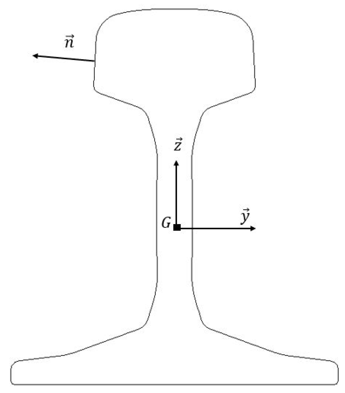
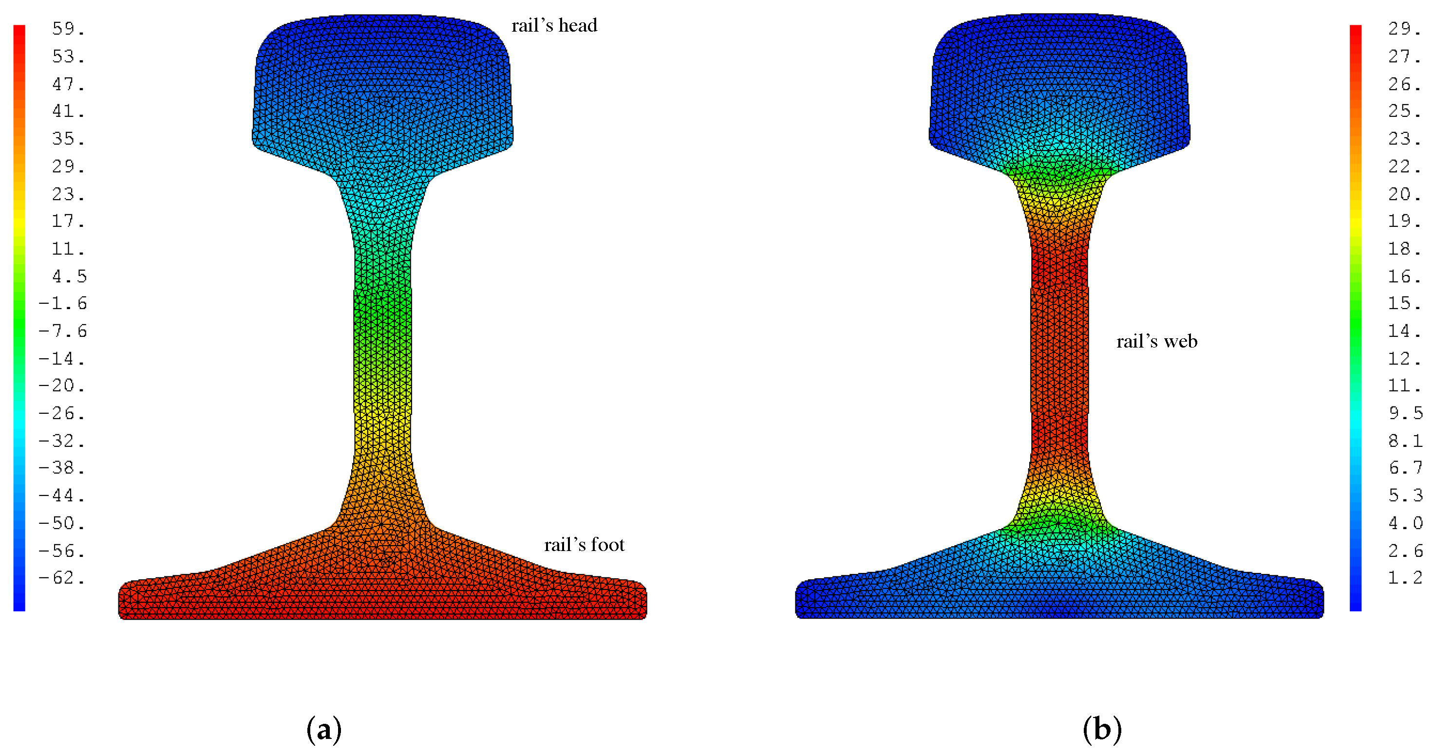
3.1.2. Stress State in the Rail

The normal and shear stress fields ( σ x x , τ ) are computed in the rail section at each node of the zone of interest ZOI and each time step using Equation (11):
σ x x ( x , z , t ) = z M y ( x , t ) I y τ ( x , y , z , t ) = T z ( x , t ) S r g ( y , z ) y 2 + T z ( x , t ) S r g ( y , z ) z 2
The determination of the shear stress τ requires computing before the warping function g ( y , z ) , independent of the value of the shear force T z . It only depends on the section itself and allows us to compute the axial warping displacement in the beam due to shear forces [41]. Classically, the warping function is the solution of the Poisson equation with a Neumann boundary condition (problem 12). The third condition in the problem formulation is to ensure the unicity of the solution.
Δ g = z S r I y ( in all the domain S r ) g y n y + g z n z = 0 ( null Neuman condition on the boundary of S r ) S r g d s = 0 ( unicity condition )
where z S r I y is a source term equivalent to a surface loading, n y and n z are the directional cosines of the rail section edge’s normal vector n defined in the principal coordinate system ( G , x , y , z ) , G being the center of gravity of the rail section as reported in Figure 8.
Unlike regular sections, the analytical computation of the warping function g ( y , z ) for the rail section is not possible. In this study, it is computed using the finite element method. The rail section is discretised into triangular linear plane elements, and the system (12) is solved by taking advantage of a thermic analogy observed in the stationary heat equation ( D Δ T = R , D is the conductivity matrice and T is the temperature field). Indeed, the implemented method consists of solving a fictive thermic problem for the meshed rail section. The conductivity coefficient is set to 1 to respect the equation form in the problem (12) and the source term is R = z S r I y . A fictive mass matrice is constructed to convert integral writing of quantities to matrice writing, which is useful in the finite element method. As an example, the y coordinate of the rail centre of gravity is written as:
y G = 1 S r S r y d S
Using finite element method, the y coordinates on the rail section are known at the level of mesh nodes. Thus, the y i = 1 : N n coordinate vector of the mesh is written, where N n is the number of nodes. The y coordinate of the center of gravity G becomes:
y G = 1 S r S r 1 N ( y , z ) y i = 1 : N n d S
where N i ( x , y ) are the shape functions and 1 is a unit function that can be expressed as:
1 = N ( y , z ) U = 1 T = U T N ( y , z ) T U = 1 i = 1 : N n
Finally, the y coordinate of the center of gravity G is expressed as:
y G = 1 S r U T M y i = 1 : N n
where M is the fictive mass matrice in question for a unit density:
M = S r N ( y , z ) T N ( y , z ) d S
The stress history of a rail Section P is examined. It is the first section located between two sleepers right after the mid-length point on the rail, as shown in Figure 9a. More specifically, Figure 9b shows the time evolution of the maximum stresses in this section P max ( y , z ) P σ x x and max ( y , z ) P τ . The shear stress and normal stress are seen to have the same order of magnitude. Obviously, the highest value of normal stress is observed when each vehicle’s wheel reaches Section P (the peak is observed under the wheel’s load). However, shear stress peaks are observed on both sides of the wheel’s load position due to the shear load discontinuity. It means that for Section P, the maximum shear stress is observed when a wheel is located in the previous Section P − 1 and when it is located in the following Section P + 1. The normal and shear stress fields in the rail section are hence shown in Figure 10 when the shear stress is maximum at the fourth peak. More specifically, extreme values of the normal stress are located on the rail’s foot (tension) and the rail’s head (compression). However, the shear stress is maximum in the rail’s web.

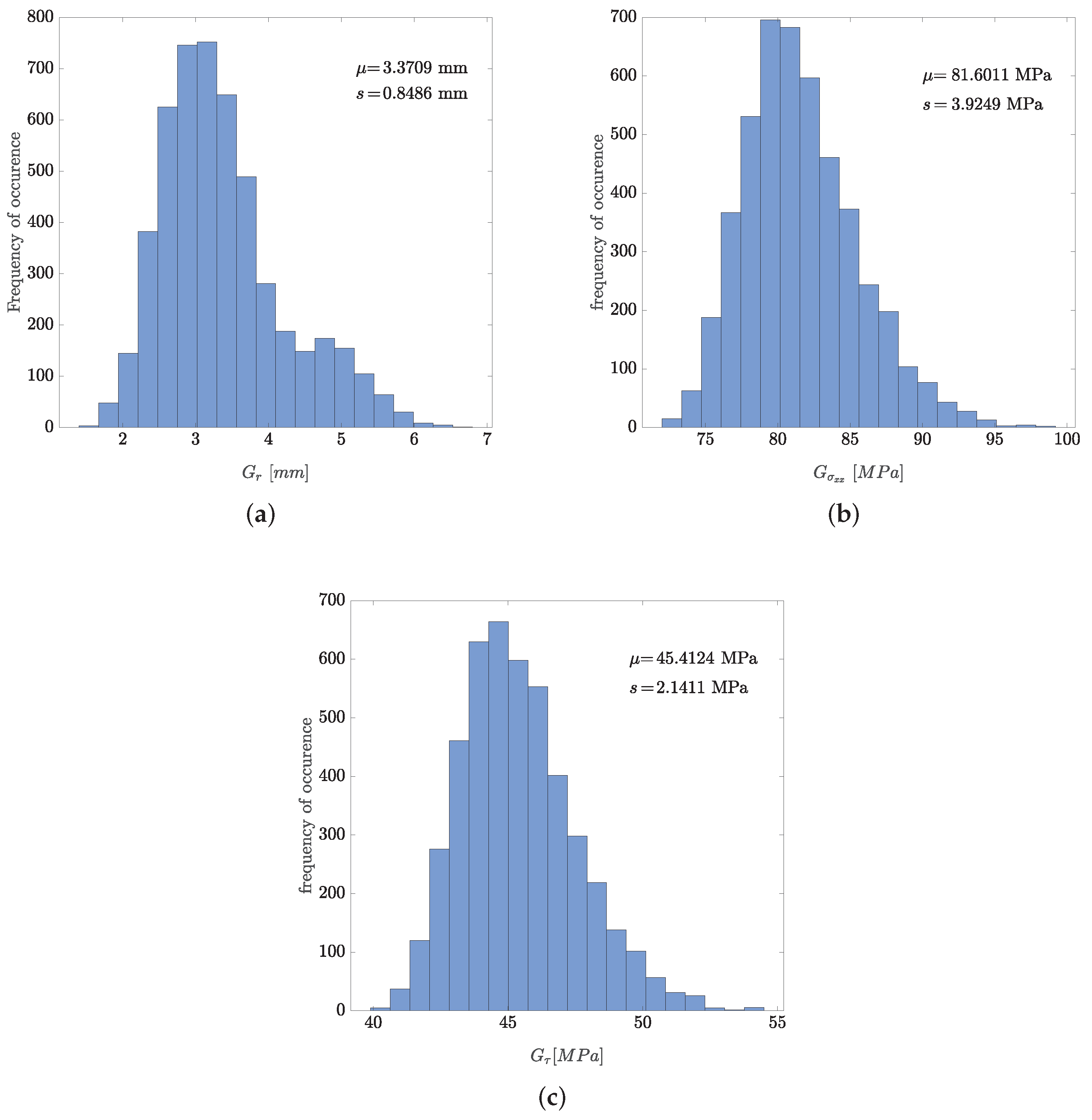
3.2. Statistical Analysis

A statistical analysis is realised in order to study the effect of the track irregularity variability on the rail’s stress response variability.
In accordance with Section 2.2.1, 5000 vertical track irregularities random samples are generated. One recalls that the random nature of the vertical track irregularity comes from the random phases. The random variable G r relative to the vertical track irregularity is chosen as the maximum amplitude along the track (Equation (18)).
G r = max x | r ( x ) |
Then, for each track irregularity sample, the maximum normal stress and the maximal shear stress in the rail with respect to time and space are computed:
G σ x x = max x , y , z , t | σ x x ( x , y , z , t ) | G τ = max x , y , z , t | τ ( x , y , z , t ) |
Distributions of the three random variables are presented in Figure 11.
The coefficient of variation C V is then computed for each distribution. Indeed, it allows for the characterisation of the relative dispersion of the samples with respect to the mean’s distribution μ :
C V = s μ
where s is the standard deviation of the distribution. The coefficients of variation associated with the vertical track irregularity and stress variables are reported in Table 2. Indeed, low values are obtained for the normal and shear stress variables compared to the track defect variable. It shows that the track defect dispersion does not affect the stress state as an output. Therefore, the stress state in the rail due to vertical loads of the vehicle can be characterised through one deterministic simulation of the numerical vehicle’s model and the track’s model.

4. Conclusions

In this paper, a lightweight and efficient finite element model of the track and a simplified multi-body model of the vehicle were implemented to analyse the vertical response of the rail under a moving vehicle in the context of the development of an efficient methodology to support the railway vehicle admission procedure in the French railway network. The frequency range of interest being in [0;20 Hz], the track model was uncoupled from the vehicle model as the track’s dynamic is negligible in front of the vehicle’s dynamic, and it has no impact on it. A random irregularity of the track vertical profile was generated from defect measurements on the French railway network. It was assimilated to an excitation source of the vehicle system to compute dynamic vehicle overloads. The normal and shear stresses were determined in the rail. It required the computation of the rail’s section warping function using the finite element method to estimate the shear stress.
A first investigation intending to compare the dynamic and static responses of the track showed negligible effects of track inertia forces on its response. Indeed, the track’s stiffness is more important than the vehicle’s stiffness in the vertical direction. The track’s natural frequencies are higher than the frequency domain of interest [0;20 Hz], in which dynamic railway phenomena are studied. Then, the stress state in the rail showed that normal and shear stresses have the same order of magnitude because the distance between two consecutive sleepers is relatively low compared to the section size. Finally, a statistical analysis aimed to quantify the effect of the vertical track irregularity variability on the rail’s stress response variability. It showed that track defect dispersion does not affect the stress state as an output, meaning that the stress response of the rail is relatively insensitive to the variability of vertical track irregularities.

5. Perspectives

Further investigations are intended to characterise the track’s lateral behaviour. This will be performed by adapting both the vehicle and track model to 3D loads and irregularities. Unlike the vertical direction, the dynamic response of the track in the lateral response is expected to be significant as the track is more flexible and less damped than in the vertical direction. Then, fatigue analysis of the rail can be predicted using the Dang Van Criterion. This will allow for the demonstration of the method in real practice for real vehicles used on French railways. A comparison with the conventional approach must also be performed. Thus, new admission rules based on this efficient numerical model can be formulated.

Author Contributions

Conceptualization, M.E.M., F.L., P.-A.B. and F.D.; methodology, M.E.M., F.L. and P.-A.B.; software, M.E.M. and F.L.; validation, M.E.M., F.L. and P.-A.B.; formal analysis, M.E.M.; investigation, M.E.M.; resources, F.L., P.-A.B. and F.D.; data curation, M.E.M., F.L., P.-A.B. and F.D.; writing—original draft preparation, M.E.M.; writing—review and editing, M.E.M.; visualisation, M.E.M.; supervision, F.L., P.-A.B., F.D., G.S. and D.S.; project administration, F.L., P.-A.B. and F.D.; funding acquisition, F.D., G.S. and D.S. All authors have read and agreed to the published version of the manuscript.

Funding

This work was partially funded by the ANRT (Association Nationale de la Recherche et de la Technologie).

Conflicts of Interest

The authors declare no conflict of interest.

Appendix A. Recall of the Finite Element Matrices of a Two Nodes Timoshenko Beam

Finite element theory allows us to interpolate the vertical displacement and the rotation in an element with respect to linear independant shape functions vector N i ( x ) :
v r ( x ) θ r ( x ) = N 1 ( x ) 0 N 2 ( x ) 0 0 N 3 ( x ) 0 N 4 ( x ) v r , 1 θ r , 1 v r , 2 θ r , 2 = ( 1 x l e ) 0 x l e 0 0 ( 1 x l e ) 0 x l e v r , 1 θ r , 1 v r , 2 θ r , 2
where l e is the element length. Then, the deformations ϵ x x and γ x z are expressed as:
ϵ x x = z θ r x = z 0 N 3 x 0 N 4 x v r , 1 θ r , 1 v r , 2 θ r , 2 = z { B F } v r , 1 θ r , 1 v r , 2 θ r , 2 γ x z = v r x θ r = N 1 x N 3 N 2 x N 4 v r , 1 θ r , 1 v r , 2 θ r , 2 = { B S } v r , 1 θ r , 1 v r , 2 θ r , 2
For a Timoshenko beam element, the stiffness matrix is a contribution of shear and bending:
[ K r e ] = E I y 0 l e { B F } T { B F } d x + G κ z S r 0 l e { B S } T { B S } d x = E I y l e 0 0 0 0 0 1 0 1 0 0 0 0 0 1 0 1 + G κ z S r l e 1 l e 2 1 l e 2 l e 2 l e 2 3 l e 2 l e 2 6 1 l e 2 1 l e 2 l e 2 l e 2 6 l e 2 l e 3 3
where κ z is the shear coefficient. The rail mass matrix is expressed as follows:
[ M r e ] = m r S r 0 l e { N } T { N } d x = l e 6 m r S r 2 2 1 1 2 2 1 1 1 1 2 2 1 1 2 2
Global mass matrix and global stiffness matrix of the rail are then obtained by assembling element matrices.
The beam elements of the rail in contact with the rail pads are vertically connected to the ground through the sleeper by spring-damper couples representing the behaviour of rail-pads and the ballast layer. In this way, the rail vertical deflections v r , i and the sleepers vertical deflections v s , j are involved. The stiffness, damping and mass matrix of a single elastic support are then represented by:
[ K s u p ] = k p k p k p k b + k p ; [ C s u p ] = c p c p c p c b + c p ; [ M s u p ] = 0 0 0 M s
where M s is the half-mass of a single sleeper.

References

  1. SNCF. Règles D’admission des Matériels Roulants sur le RFN en Fonction de la Sollicitation de la Voie; Internal Report; SNCF Division Interaction Véhicule Voie: La Plaine Saint-Denis, France, 2019. [Google Scholar]
  2. Kraft, S. Parameter Identification for a TGV Model. Ph.D. Thesis, Ecole Centrale de Paris, Paris, France, 2012. [Google Scholar]
  3. SNCF. Rapport de la Commission Demaux; Internal Report; SNCF: Paris, France, 1944. [Google Scholar]
  4. Ling, L.; Xiao, X.B.; Xiong, J.Y.; Zhou, L.; Wen, Z.F.; Jin, X.S. A 3D model for coupling dynamics analysis of high-speed train/track system. In China’s High-Speed Rail Technology; Springer: Singapore, 2018; pp. 309–339. [Google Scholar]
  5. Xu, Y.; Yang, C.; Zhendong, L.; Zhang, W.; Stichel, S. Long-Term High-Speed Train-Track Dynamic Interaction Analysis. In Proceedings of the 27th IAVSD Symposium on Dynamics of Vehicles on Roads and Tracks, Saint-Petersburg, Russia, 16–20 August 2021. [Google Scholar]
  6. Cai, W.; Chi, M. Study on steady-state responses of high-speed vehicle using infinite long track model. Shock Vib. 2020, 2020, 6878252. [Google Scholar] [CrossRef]
  7. Mei, H.; Leng, W.; Nie, R.; Liu, W.; Chen, C.; Wu, X. Random distribution characteristics of peak dynamic stress on the subgrade surface of heavy-haul railways considering track irregularities. Soil Dyn. Earthq. Eng. 2019, 116, 205–214. [Google Scholar] [CrossRef]
  8. Varandas, J.N.; Paixão, A.; Fortunato, E.; Coelho, B.Z.; Hölscher, P. Long-term deformation of railway tracks considering train-track interaction and non-linear resilient behaviour of aggregates—A 3D FEM implementation. Comput. Geotech. 2020, 126, 103712. [Google Scholar] [CrossRef]
  9. Sayeed, M.A.; Shahin, M.A. Three-dimensional numerical modelling of ballasted railway track foundations for high-speed trains with special reference to critical speed. Transp. Geotech. 2016, 6, 55–65. [Google Scholar] [CrossRef] [Green Version]
  10. Chebli, H.; Clouteau, D.; Schmitt, L. Dynamic response of high-speed ballasted railway tracks: 3D periodic model and in situ measurements. Soil Dyn. Earthq. Eng. 2008, 28, 118–131. [Google Scholar] [CrossRef]
  11. Arlaud, E. Modèles Dynamiques Réduits de Milieux Périodiques par Morceaux: Application aux Voies Ferroviaires. Ph.D. Thesis, École Nationale Supérieure d’Arts et Métiers, Paris, France, 2016. [Google Scholar]
  12. Rhayma, N.; Bressolette, P.h.; Breul, P.; Fogli, M.; Saussine, G. A probabilistic approach for estimating the behavior of railway tracks. Eng. Struct. 2011, 33, 2120–2133. [Google Scholar] [CrossRef]
  13. Fernandes, V.A.; Lopez-Caballero, F.; d’Aguiar, S.C. Probabilistic analysis of numerical simulated railway track global stiffness. Comput. Geotech. 2014, 55, 267–276. [Google Scholar] [CrossRef]
  14. Xie, G.; Iwnicki, S.D. Simulation of wear on a rough rail using a time-domain wheel–track interaction model. Wear 2008, 265, 1572–1583. [Google Scholar] [CrossRef]
  15. Nielsen, J.C.; Igeland, A. Vertical dynamic interaction between train and track influence of wheel and track imperfections. J. Sound Vib. 1995, 187, 825–839. [Google Scholar] [CrossRef]
  16. Ferrara, R.; Leonardi, G.; Jourdan, F. Numerical modelling of train induced vibrations. Procedia Soc. Behav. Sci. 2012, 53, 155–165. [Google Scholar] [CrossRef]
  17. Hou, K.; Kalousek, J.; Dong, R. A dynamic model for an asymmetrical vehicle/track system. J. Sound Vib. 2003, 267, 591–604. [Google Scholar] [CrossRef]
  18. Sun, Y.Q.; Dhanasekar, M. A dynamic model for the vertical interaction of the rail track and wagon system. Int. J. Solids Struct. 2002, 39, 1337–1359. [Google Scholar] [CrossRef]
  19. Zhang, Q.L.; Vrouwenvelder, A.; Wardenier, J. Numerical simulation of train–bridge interactive dynamics. Comput. Struct. 2001, 79, 1059–1075. [Google Scholar] [CrossRef]
  20. Lei, X.; Noda, N.A. Analyses of dynamic response of vehicle and track coupling system with random irregularity of track vertical profile. J. Sound Vib. 2002, 258, 147–165. [Google Scholar] [CrossRef]
  21. Au, F.T.K.; Wang, J.J.; Cheung, Y.K. Impact study of cable-stayed railway bridges with random rail irregularities. Eng. Struct. 2002, 24, 529–541. [Google Scholar] [CrossRef]
  22. Wang, Y.; Dimitrovová, Z.; Yau, J. Dynamic responses of vehicle ballasted track interaction system for heavy haul trains. MATEC Web Conf. 2018, 148, 05004. [Google Scholar] [CrossRef] [Green Version]
  23. Arvidsson, T.; Andersson, A.; Karoumi, R. Train running safety on non-ballasted bridges. Int. J. Rail Transp. 2019, 7, 1–22. [Google Scholar] [CrossRef] [Green Version]
  24. Martínez-Rodrigo, M.D.; Galvín, P.; Moliner, E.; Romero Ordóñez, A. Rail-Bridge Interaction Effects in Single-Track Multi-Span Bridges. Experimental Results versus Numerical Predictions under Operating Conditions. In Proceedings of the XI International Conference on Structural Dynamics, EURODYN 2020, Athens, Greece, 23–26 November 2020; Papadrakakis, M., Fragiadakis, M., Papadimitriou, C., Eds.; Institute of Structural Analysis and Antiseismic Research, School of Civil Engineering, National Technical University of Athens (NTUA): Athens, Greece, 2020; Volume I, pp. 1652–1665, ISBN 978-618-85072-0-3. [Google Scholar]
  25. Shan, Y.; Wang, B.; Zhang, J.; Zhou, S. The influence of dynamic loading and thermal conditions on tram track slab damage resulting from subgrade differential settlement. Eng. Fail. Anal. 2021, 128, 105610. [Google Scholar] [CrossRef]
  26. Punetha, P.; Nimbalkar, S.; Khabbaz, H. Simplified geotechnical rheological model for simulating viscoelasto-plastic response of ballasted railway substructure. Int. J. Numer. Anal. Methods Geomech. 2021, 45, 2019–2047. [Google Scholar] [CrossRef]
  27. Dimitrovová, Z. Two-layer model of the railway track: Analysis of the critical velocity and instability of two moving proximate masses. Int. J. Mech. Sci. 2022, 217, 107042. [Google Scholar] [CrossRef]
  28. Sysyn, M.; Przybylowicz, M.; Nabochenko, O.; Liu, J. Mechanism of Sleeper–Ballast Dynamic Impact and Residual Settlements Accumulation in Zones with Unsupported Sleepers. Sustainability 2021, 13, 7740. [Google Scholar] [CrossRef]
  29. Sysyn, M.; Przybylowicz, M.; Nabochenko, O.; Kou, L. Identification of Sleeper Support Conditions Using Mechanical Model Supported Data-Driven Approach. Sensors 2021, 21, 3609. [Google Scholar] [CrossRef] [PubMed]
  30. Knothe, K.L.; Grassie, S.L. Modelling of railway track and vehicle/track interaction at high frequencies. Veh. Syst. Dyn. 1993, 22, 209–262. [Google Scholar] [CrossRef]
  31. Iwnicki, S. Handbook of Railway Vehicle Dynamics; CRC Press: Boca Raton, FL, USA, 2006; pp. 147–165. [Google Scholar]
  32. Dumitriu, M. Analysis of the dynamic response in the railway vehicles to the track vertical irregularities. Part II: The numerical analysis. J. Eng. Sci. Technol. 2015, 8, 32–39. [Google Scholar] [CrossRef]
  33. Guerin, N. Approche Expérimentale et Numérique du Comportement du Ballast des Voies Ferrées. Ph.D. Thesis, École Nationale des Ponts et Chaussées, Champs-sur-Marne, France, 1996. [Google Scholar]
  34. Paixão, A.; Fortunato, E.; Calçada, R. The effect of differential settlements on the dynamic response of the train–track system: A numerical study. Eng. Struct. 2015, 88, 216–224. [Google Scholar] [CrossRef]
  35. Xu, L.; Zhai, W.; Gao, J. Extended applications of track irregularity probabilistic model and vehicle–slab track coupled model on dynamics of railway systems. Veh. Syst. Dyn. 2017, 88, 1686–1706. [Google Scholar] [CrossRef]
  36. Perrin, G.; Soize, C.; Duhamel, D.; Funfschilling, C. Track irregularities stochastic modeling. Probabilistic Eng. Mech. 2013, 34, 123–130. [Google Scholar] [CrossRef] [Green Version]
  37. Newmark, N.M. A method of computation for structural dynamics. J. Eng. Mech. 1959, 85, 67–94. [Google Scholar] [CrossRef]
  38. Cast3M. Available online: http://www-cast3m.cea.fr (accessed on 30 March 2022).
  39. Nguyen, V.H. Comportement Dynamique de Structures Non-Linéaires Soumises à des Charges Mobiles. Ph.D. Thesis, École Nationale des Ponts et Chaussées, Champs-sur-Marne, France, 2002. [Google Scholar]
  40. Cai, Z.; Raymond, G.P.; Bathurst, R.J. Natural vibration analysis of rail track as a system of elastically coupled beam structures on Winkler foundation. Comput. Struct. 1994, 53, 1427–1436. [Google Scholar] [CrossRef]
  41. Cambronero-Barrientos, F.; Díaz-del-Valle, J.; Martínez-Martínez, J.A. Beam element for thin-walled beams with torsion, distortion, and shear lag. Eng. Struct. 2017, 143, 571–588. [Google Scholar] [CrossRef]
Figure 1. Finite element model of the track.
Vibration 05 00019 g001
Figure 2. Degrees of freedom of a rail beam element.
Vibration 05 00019 g002
Figure 3. Mauzin car. Reproduced with permission from Jérémie Badinos and Thierry Vicol (SNCF Réseau); photo taken by Jérémie Badinos and Thierry Vicol, 2016.
Vibration 05 00019 g003
Figure 4. Simplified multi-body model of a railway half-vehicle (i.e., only one rail of the track is modelled).
Vibration 05 00019 g004
Figure 5. Random vertical track irregularity profile and its associated vehicle’s dynamic overloads. (a) Generated vertical track irregularity in the wavelength domain λ [3;30 m].; (b) Dynamic vehicle’s loads associated with the track defect for a vehicle speed of V = 216 km/h.
Vibration 05 00019 g005
Figure 6. Comparison of the dynamic and static responses of the track in the mid-region of the track ZOI when the vehicle reaches the rail mid-length. (a) Vertical displacement. (b) Bending moment. (c) Shear force.
Vibration 05 00019 g006
Figure 7. L norm error used to quantify the gap between the static and the dynamic responses of the track in its mid-region ZOI. (a) For vertical displacement. (b) For bending moment. (c) For shear force.
Vibration 05 00019 g007
Figure 8. Rail section edge: representation of its associated coordinate system ( G , x , y , z ) and the unitary normal vector to the rail section edge n .
Vibration 05 00019 g008
Figure 9. Stress history of a given rail Section P due to the moving vehicle. (a) Position of the rail Section P with respect to the track length. (b) Time evolution of the Maximum normal stress max ( y , z ) P σ x x and maximum shear stress max ( y , z ) P τ in Section P.
Vibration 05 00019 g009
Figure 10. Stress field in Section P when the fourth wheel reaches the section (i.e., at the time of the fourth peak in Figure 9b). (a) Normal stress σ x x [MPa]. (b) Shear stress τ [MPa].
Vibration 05 00019 g010
Figure 11. Statistical distribution of the vertical irregularity and stresses random variables. (a) Vertical irregularity variable G r . (b) Normal stress variable G σ x x . (c) Shear stress variable G τ .
Vibration 05 00019 g011
Table 1. Track [14] and vehicle parameters.
ParameterNotationNumerical Value
-Track system-
Rail density ρ r 7850 kg m 3
Rail Young’s modulusE 210 × 10 3 MPa
Rail cross section S r 7.67 × 10 3 m 2
Rail second moment of area I y 3.0383 × 10 6 m 4
Rail-pad vertical stiffness k p 350 M N m 1
Rail-pad vertical damping c p 50 MN s m 1
Half sleeper mass M s 162 kg
Sleeper spacingl 0.6 m
Ballast vertical stiffness k b 50 MN m 1
Ballast vertical damping c b 100 MN s m 1
-Half Vehicle system-
Half car body mass M c 23,400 kg
Half car body pitch moment of inertia J c 965,979.7 kg m 2
Half bogie mass M b 6742.5 kg
Half bogie pitch moment of inertia J b 5606.9 kg m 2
Wheel mass M w 1902.5 kg
Primary suspension vertical stiffness k z 1 7.32565 MN m 1
Primary suspension vertical damping c z 1 38.44 kN s m 1
Secondary suspension vertical stiffness k z 2 1.2313 MN m 1
Secondary suspension vertical damping c z 2 7.8164 kN s m 1
Secondary suspension pitch stiffness k θ 0.0098235 MN m r d 1
Secondary suspension pitch damping c θ 0.87128 kN m s r d 1
Wheel base d w 2.8 m
Distance between the two bogie centrelines d b 9.7 m
Table 2. Coefficients of variation of the vertical irregularity, maximum normal stress and maximum shear stress random variables.
CV r [ % ] CV σ xx [ % ] CV τ [ % ]
25.18 4.81 4.71
Publisher’s Note: MDPI stays neutral with regard to jurisdictional claims in published maps and institutional affiliations.

