SNAPScapes: Using Geodemographic Segmentation to Classify the Food Access Landscape


Department of Geography and Earth Sciences, University of North Carolina at Charlotte, Charlotte, NC 20836, USA
*
Authors to whom correspondence should be addressed.
Urban Sci. 2018, 2(3), 71; https://doi.org/10.3390/urbansci2030071
Submission received: 14 July 2018
/
Revised: 10 August 2018
/
Accepted: 13 August 2018
/
Published: 21 August 2018
(This article belongs to the Special Issue Urban Food Security)
Abstract
:Scholars are in agreement that the local food environment is shaped by a multitude of factors from socioeconomic characteristics to transportation options, as well as the availability and distance to various food establishments. Despite this, most place-based indicators of “food deserts”, including those identified as so by the US Department of Agriculture (USDA), only include a limited number of factors in their designation. In this article, we adopt a geodemographic approach to classifying the food access landscape that takes a multivariate approach to describing the food access landscape. Our method combines socioeconomic indicators, distance measurements to Supplemental Nutrition Assistance Program (SNAP) participating stores, and neighborhood walkability using a k-means clustering approach and North Carolina as a case study. We identified seven distinct food access types: three rural and four urban. These classes were subsequently prioritized based on their defining characteristics and specific policy recommendations were identified. Overall, compared to the USDA’s food desert calculation, our approach identified a broader swath of high-needs areas and highlights neighborhoods that may be overlooked for intervention when using simple distance-based methods.
1. Introduction
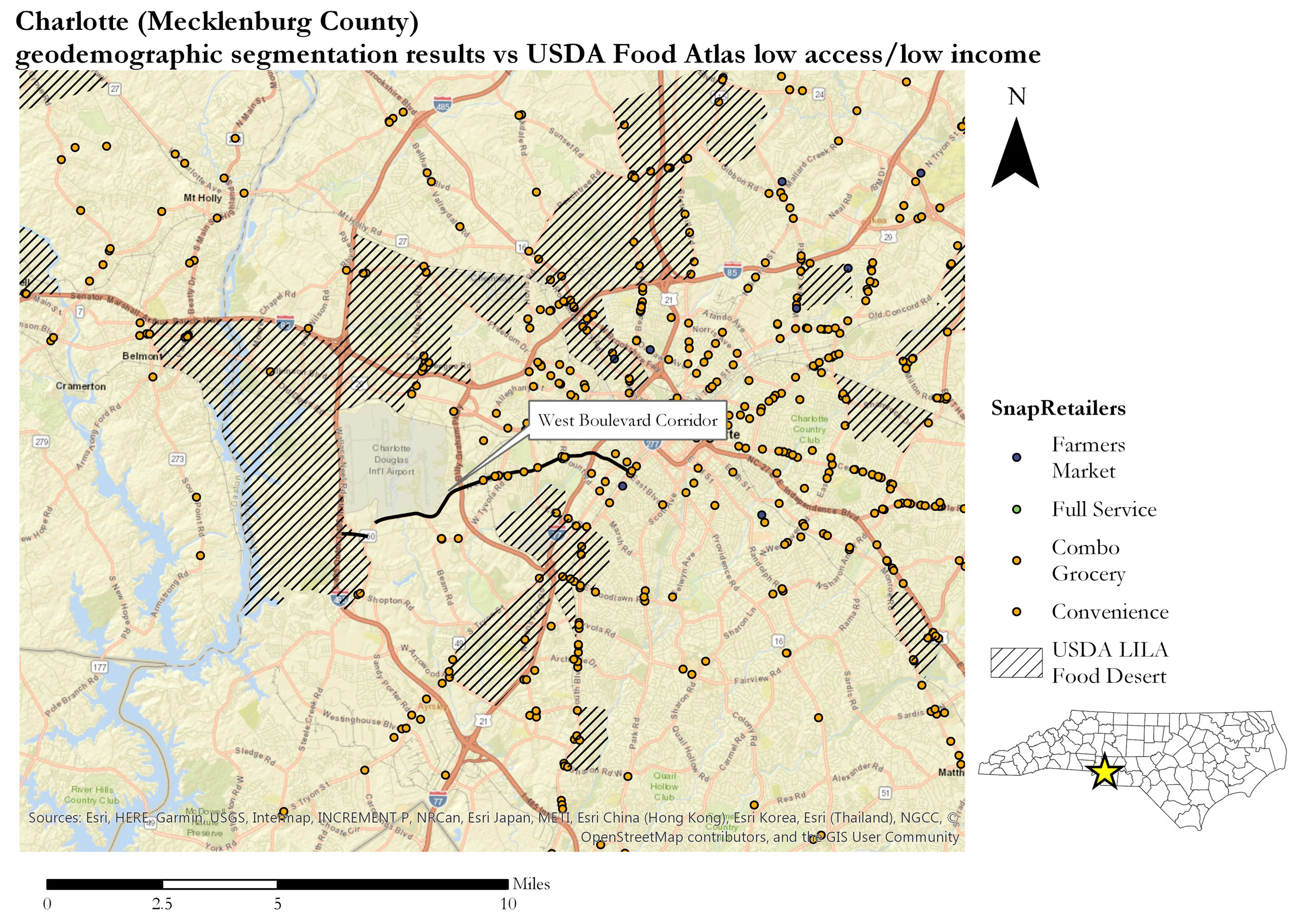
On 16 March 2017, The Charlotte Observer published an article highlighting the lack of grocery stores in the West Boulevard Corridor, a predominantly African-American neighborhood west of Charlotte’s city center (see Figure 1) [1]. In the article, the authors describe the route Tribonia Ponder takes to buy food for herself: “Ponder, who lives off of West Boulevard and does not have a car, typically takes the No. 10 bus uptown, then transfers to the No. 2, which drops her off at the Walmart Supercenter on Wilkinson Boulevard” [1]. It takes Ponder approximately an hour to get to the store, and an hour to return home with her groceries. The corridor is one of three areas identified in the Charlotte-Mecklenburg Food Policy Council’s State of the Plate initiative as a “high food insecurity risk area”. By their definition, a food-insecure household is one where a job loss or disruption in transportation could restrict that household’s access to healthy food. “Most food insecurity is episodic, not chronic. Hunger is not a huge problem in Charlotte, but food insecurity is… Maybe you lost your job and had to sell your car. Or suddenly you’re not working, so now you have to go far outside your neighborhood to buy milk” says Katherine Metzo, who co-authored the report. Metzo implies that access hinges on more than having the ability to purchase quality food at a fair price—you also need to be able to get to it. Local food environments—comprised of the nearby stock of grocery stores, convenience stores, and restaurants—are highly variable landscapes with a range of goods available. The quality of these goods is often tied to the socioeconomics of the area, with more disadvantaged areas tending to predict worse food options [2,3].
The most comprehensive classification of food environments in the United States is the US Department of Agriculture (USDA) Food Access Research Atlas, in which they publish a Food Desert Locator Map [4]. The USDA defines food deserts as “a part of the country vapid of fresh fruit, vegetables, and other healthy whole foods, usually found in impoverished areas” [5], measured at census tract level. The USDA identifies tracts they have found to be “low-income/low-access” (LILA) food deserts at a series of distance thresholds, the most common being one mile for urban areas and ten miles for rural. The USDA’s low-income/low-access tracts are a first step for researchers intending to explore food access in the United States. In Charlotte, most of the West Boulevard Corridor, however, is not represented on the Food Desert Locator as a LILA (Figure 1). This example, as well as recent work in the area of food access, calls the effectiveness of the USDA’s metric into question. If food insecurity is indeed episodic and caused by a number of factors, then food access metrics should account for more than just income and absolute distance to a store.
Recent articles published on the topic of food access have considered a broad range of techniques to observe different aspects of food inaccessibility including transit and daily mobility data [6,7,8,9,10], food diaries and surveys to investigate consumer behavior [11,12], and descriptive studies of food stores and the quality and pricing of their content [13,14]. This literature has consistently called into question the accuracy of food desert studies that only account for the minimum distance to a grocery store and do not consider daily patterns of mobility, citing the multidimensionality of food access and consumer behavior. The decisions that individuals or families make to determine what to buy, where to buy, how much to spend, and how to get to the store are complex and require more nuanced investigation. The local food environment, in turn, is shaped by socioeconomic circumstances of the neighborhood, the availability and variety of food stores, and the accessibility to them. From a policy perspective, the unique combination of these factors can give rise to place-specific remedies that address the particular conditions of that neighborhood.
In light of the multidimensionality of food insecurity, in this article, we implement a geodemographic segmentation approach to examine and map the food access landscape. This problem-specific geodemographic segmentation sorts neighborhoods according to their demographics, walkability, minimum distance to several varieties of food stores, and the concentration of food stores in the immediate vicinity. By following this multivariate approach, we create a data-rich portrait of local food environments that demonstrates their variability, revealing the types of food options that are in abundance as well as the ones that are missing. Further, we increase specificity (particularly in rural areas) by operating at a finer scale than the one used by the USDA and provide a method that utilizes recent and freely available data sources thereby ensuring the replicability across the United States. This place-based classification therefore addresses some of the limitations of the USDA’s singular metric definition and encompasses a broader set of factors in identifying food-insecure areas than those that focus on a single dimension of this issue [6,8].
In this analysis, we place particular emphasis on individuals taking part in the USDA Supplemental Nutrition Assistance Program (SNAP) using SNAP-approved stores to generate routes and store counts, and including demographic information related to SNAP in the clustering process. The SNAP program constitutes a large part of the federal safety net, and until recently participation in the program tracked with the federal unemployment rate. Approximately one in seven Americans buys groceries with the help of SNAP benefits [15]. To many of the most vulnerable, a store that does not participate in the SNAP program is not an accessible store, and areas with high SNAP participation are likely to have the most easily disrupted access to healthy food.
We illustrate our approach on both rural and urban areas of North Carolina and address the following questions: what specific types of food access problems exist in North Carolina? How distinct are neighborhoods from each other? How does this classification align with the USDA approach? The structure of the remainder of the article is as follows: the following section provides a brief overview of the state of food access studies. The methodology and study areas are then explained followed by results and a conclusion.
2. Previous Studies and Background
2.1. Food Access
A great deal of research concerning health and equitable access has centered on access to nutritious food. Access to healthcare providers, fresh foods, and other resources are conducive to healthy lifestyles for all people. However, common business practices tend to dictate that quality food stores, recreational areas, and medical facilities accumulate near population in higher tax brackets, leaving a disadvantaged population with little or no access to these goods and services. These disparities have been well documented since the 1990s, where specific areas deemed to be “food deserts” often intersect with already disadvantaged or minority groups [16,17]. The study of food deserts has become a common practice for communities trying to improve overall health and alleviate disparities in access. These studies have commonly deployed a geographic information systems (GIS) methodology to determine areas where the distance to a food store exceeds the threshold [16,17]. Frameworks developed by the authors of early accessibility studies vary based on the area being studied or the specific questions being asked, but generally sought to find specific neighborhoods or small areas where the majority of people had low purchasing power, having to go out of their way to shop at a grocery store with fresh and healthy food [16].
In the years since the first publications on food deserts, however, the conversation has diversified from straightforward discussions of neighborhoods with no stores within a certain distance to more descriptive explorations of food environments or ecosystems. More recent studies quantify good and bad options available to residents and try to capture the complex interactions that guide food purchases within these environments. Some authors have incorporated time budgets rather than simple measures of distance to create a space-time accessibility framework [7], while others have explored individual person-based approaches that contrast with the more common place-based approaches [10]. Recent researchers have interviewed or directly observed shoppers [14], analyzed mobile GPS data to document patterns of food purchase trips [11,12], mapped flows of SNAP grocery expenditures and accessibility [13,18,19], incorporated transit schedules into their estimations of access [8] and utilized Twitter data to understand local food environments [20]. A growing consensus of researchers agree that proximity- or density-based food desert methods that only account for trips originating from place of residence oversimplify food environments and the choices offered to shoppers within them, whether they are wealthy or comparatively disadvantaged.
Space-time GIS methods, which incorporate time budgets and interaction potential models to determine where shoppers can most effectively purchase food given the time allocated to them, have become very common in recent years as they are able to account for some of the variability implied by different trip patterns [21]. Traffic data [6], road networks [7], and bus schedules [8] create highly variable food accessibility landscapes over the course of a day, which can either improve or degrade the access level depending on the circumstances. Transit itself is increasingly being considered in studies of food environments [8,9]—public transit riders face the most restricted movement and therefore usually have the most limited options when it comes to food purchases. Several transit-based food access studies have revealed complex ebbs and flows of accessibility according to both location and time of day [6,7]. Low income residents in both cases were found to have better access according to the location of transit stops, although the times which these stops were functional severely curtailed temporal access. Details like these are important to stakeholders looking to improve food access for low-income and transit-using residents but would have been overlooked by the proximity measures of the past.
2.2. Geodemographic Segmentation
Geodemographics, or geodemographic segmentation, has been simplistically described as “the study of people by where they live” ([22], p. 16). More specifically, geodemographics is predicated on the idea that there is a telling relationship between people and their place of residence. Geodemographics has historically been used as a market segmentation technique in the private sector, but several researchers have recently attempted to bring it back into the academic fold and strengthen its theoretical underpinnings [23,24,25]. In the past ten years, specialized applications of geodemographic segmentation have proven useful for a number of spatial problems, particularly health-related ones [26,27,28]. For example, county-level diabetes rates have been used to examine lifestyle groups in the United States [28] and geocoded hospital admissions data have been used to target public health campaigns in the Southwark area of London [26].
Geodemographic segmentation is a process by which many variables from separate data sources are combined into a small-area analysis to reveal distinct groups across the landscape. The diversity of data sources is valued in the case of geodemographic segmentation, rather than avoided: “As a general rule, but within limits, the more variables that are used in the clustering algorithm and the more different sources they come from the more meaningful (nuanced not idiosyncratic) the resulting set of clusters is likely to be” ([24], p. 151). Typically, transformation, weighting and redundancy-reducing methods like principal components analysis (PCA) are applied to standardize the values of the variables found in each area (frequently a neighborhood). Once they are standardized, the values for each neighborhood are segmented using an algorithm that minimizes within-group differences and maximizes between-group differences.
Two popular families of clustering methods used in geodemographic segmentation studies include hierarchal methods (such as Ward’s hierarchical clustering) and partitioning approaches. Hierarchical clustering is a bottom-up approach in which each observation begins in its own cluster. At each step of the process, observations most similar to each other in attribute distance are merged until all observations ultimately belong to the same group. Partitioning methods on the other hand, require the number of clusters to be specified at the onset of the procedure. With this approach, an initial, random centroid corresponding to the specified k number of clusters is created. Observations are then allocated to the closest of these centroids (according to their attribute similarity). Once all observations are assigned to their closest centroid, the new centroid of these initial groups is computed, and the distance between each observation and the new centroid is calculated. Observations are then reassigned to their closest centroid, and this process continues until the procedure converges and no further swapping of observations takes place [29]. While both approaches have been used in geodemographic studies, partitioning methods such as k-means are more commonly employed because of their computational efficiency as compared to hierarchical methods [29]. Despite its widespread use, k-means does have a number of limitations. Most notably, the number of clusters needs to be identified first and the results of the analysis may change depending on the location of the initial, randomly assigned location. It is therefore necessary to run the analysis multiple times to examine various clustering solutions as k varies, and to determine the stability of the solution as the initial random centroids are changed.
3. Data and Methods
3.1. Data
The food access segmentation was conducted in the state of North Carolina at the block group level. Census block groups form statistical divisions of census tracts, containing between 600 and 3000 people, and are the smallest geographical unit for which the Census Bureau regularly publishes demographic sample data in the form of American Community Survey (ACS) tables [30]. ACS data has been critiqued for its large margins of errors, particularly for small geographic units [31,32] argue that one remedy for dealing with these large standard errors is to embrace a contextual perspective that de-emphasizes single variable estimates and their associated errors and instead focuses on the characteristics of places obtained by grouping variables. The methodology adopted here addresses this recommendation by blending multiple ACS variables with additional data sources to derive a circumstantial understanding of the local food environment.
Three sources of data were used at the input for this segmentation. Socioeconomic data at the block group level comes from the US Census Bureau’s American Community Survey 5-year estimates for 2015 [30]. The initial list of 27 variables collected and evaluated from the census is summarized in Table 1.
The second source of data was an analysis of the physical access to various types of stores from each census block group [20]. Here, we selected USDA’s SNAP-approved stores categorized as full-service grocery stores (comprised of stores identified as large grocery, supermarket, or superstore), combination and convenience stores, and farmer’s markets. Distances were calculated using the MapQuest Application Programming Interface (API) to establish a network-based origin-destination matrix between the population-weighted centroid of each block group (n = 6091) to each SNAP-approved food store (n = 9580). The routes were then aggregated to the block group so that a minimum distance, minimum travel time, and store count were estimated from each block group to each type of store. These measures paint an overall picture of what kind of stores are in the proximity of the block group, and what the block group is lacking. The variables derived from this analysis are also summarized in Table 1.
The third data source was a measure of the built environment and the ease with which people can walk in that environment. Walk Score® (Washington, DC, USA, 2007) computes validated and frequently updated measures of neighborhood walkability and transit access on a scale of 0–100. Walk scores are created using a patented system of route analysis measuring pedestrian friendliness. A score was obtained for each block group’s centroid using the Walk Score API and R package.
3.2. Methods
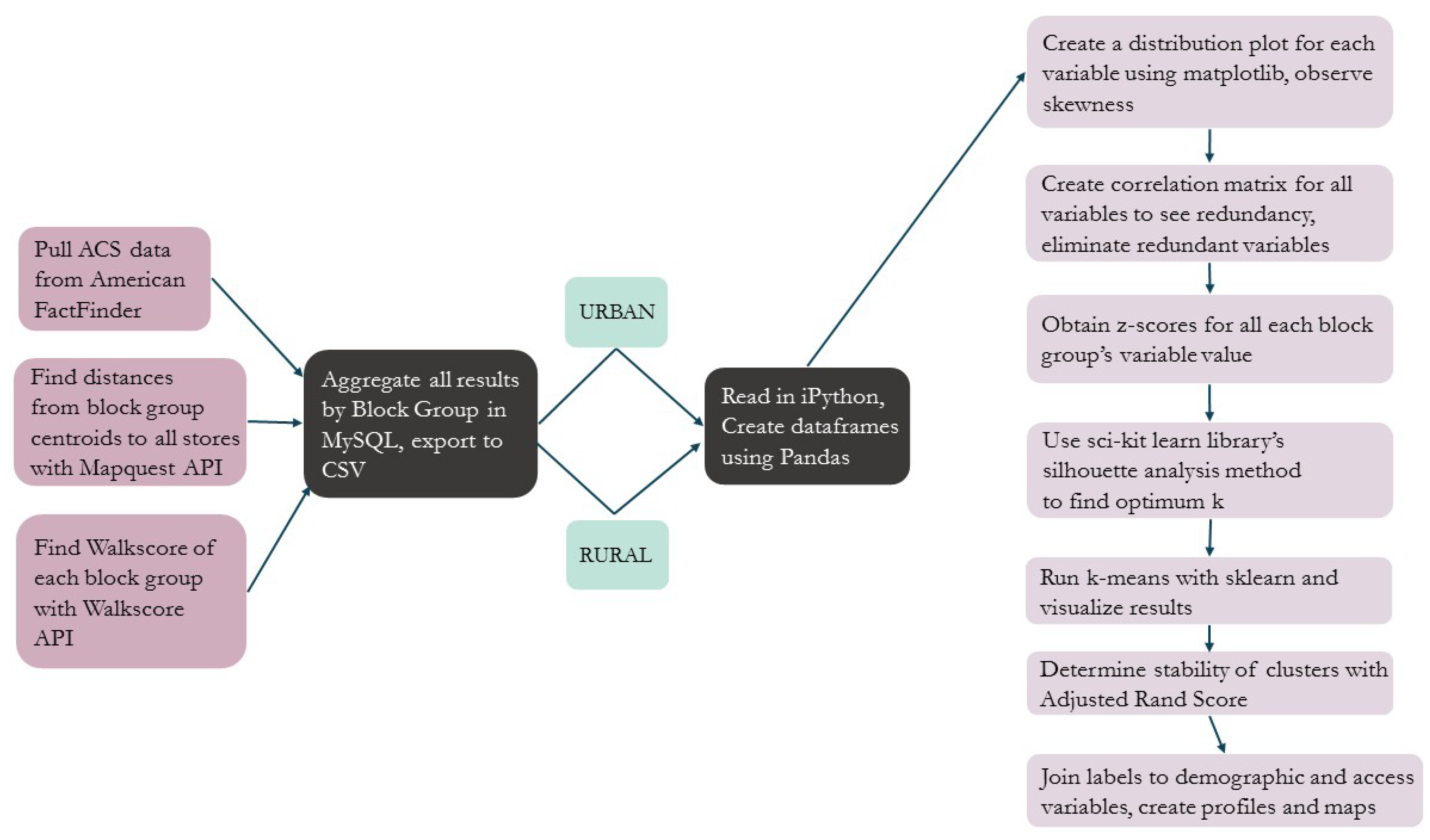
The analytical steps are illustrated in Figure 2, below and proceeded as follows. Following the data collection phase described in the previous section, the variables were aggregated to the census block group level. Because the distance thresholds and walk and transit scores were different for urban and rural block groups, the block groups were split up and variables for the two were treated separately until the final stages of the segmentation. This was to keep from losing detail: An urban block group with an unusually high number of convenience stores is still likely to have less than an average rural block group, because their distance thresholds are so different. Urban block groups were designated as so according to the US Census metropolitan statistical area definitions.
After the data were split between rural and urban areas, an initial pre-processing of the data was undertaken to check for redundancy in variables by examining their correlation. All variables were also standardized prior to entering them into the clustering procedure. The final set of selected and normalized variables were then entered into the k-means clustering algorithm where the optimal value of k was evaluated, as was the stability of the clusters. Finally, demographic and access variables for the final cluster were examined to characterize each group and create the resulting geodemographic segmentation. These steps are explained in more detail below.
3.2.1. Data Pre-Processing
Once the variables were collected from the three sources described above and in Table 1, a correlation analysis was performed to evaluate for redundancy among the initial set of indicates. Variables that show a strong correlation with other variables should not be included in the final analysis, as it would put undue emphasis on the redundant variables. The correlation analysis pointed to several redundancies and ultimately, pcHH60plus, pcSNAPdisability, pcCommuteCar, and pcCommuteCP were excluded from the analysis. After a pilot run of the k-means algorithm, all racial variables were excluded from the clustering because the algorithm created clusters that were distinct only with regard to race. In other words, their socioeconomic and access scores were very similar, but they were differentiated only by their dominant racial group. From a policy perspective, a prescription addressing a limitation of the local food environment should be the same regardless of the racial composition of the neighborhood. Of the initial twenty-seven variables collected, eighteen were used in the final clustering. In order to use variables based on different measurement scales in the clustering procedure, all variables were standardized by creating a z-score and these standardized variables were used in the analysis.
3.2.2. k-Means Analysis
Because the initial k-means assignment of categories is random, it impacts the results and it is therefore critical to run the analysis multiple times and compare until the results converge. In this case, the analysis was repeated 1000 times for both the urban and rural segmentations. The run that minimized the squared distance the most was selected as the final clustering solution [33]. The k-means clustering in this analysis was completed in Python using the machine learning library scikit-learn [34].
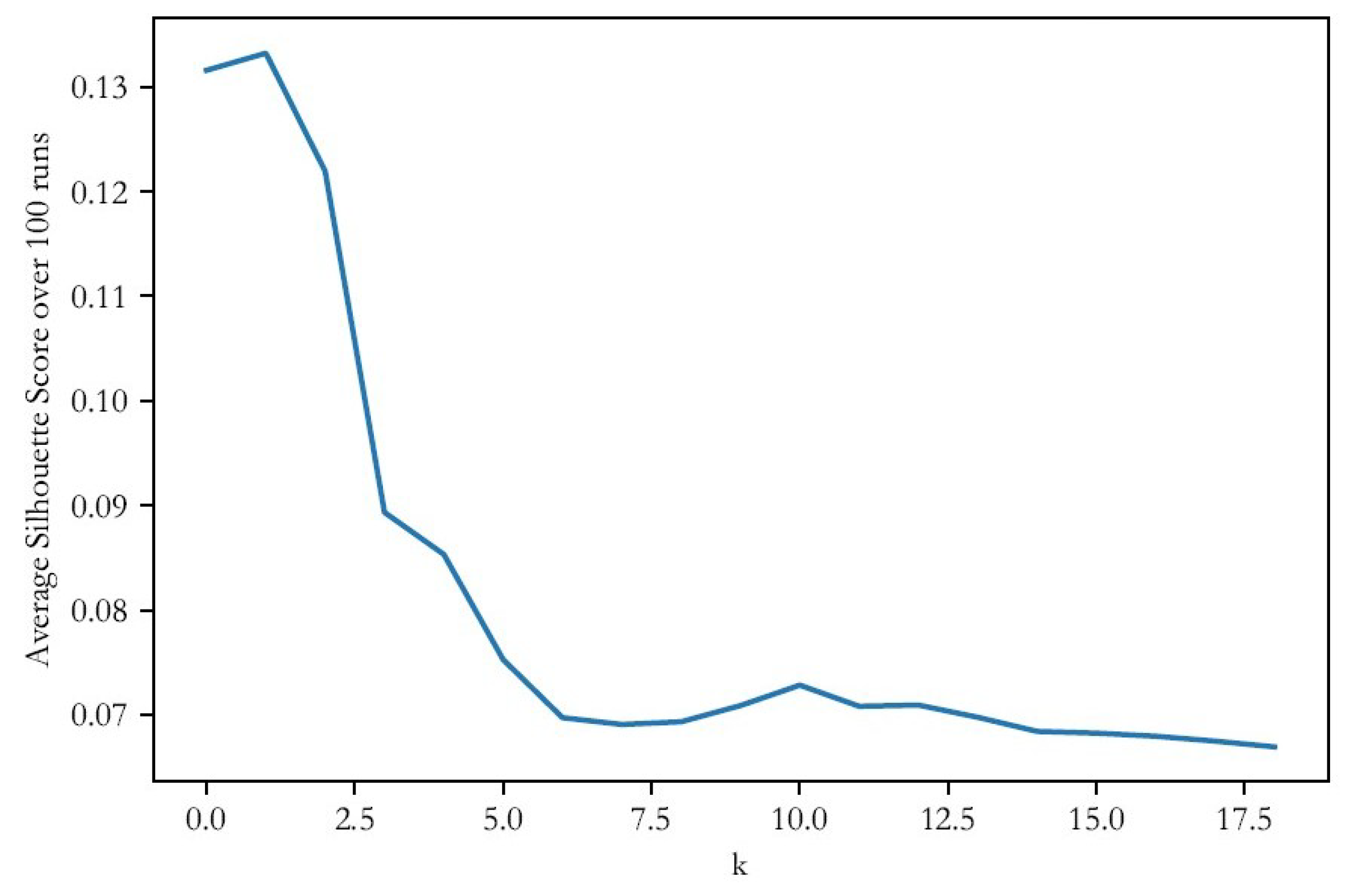
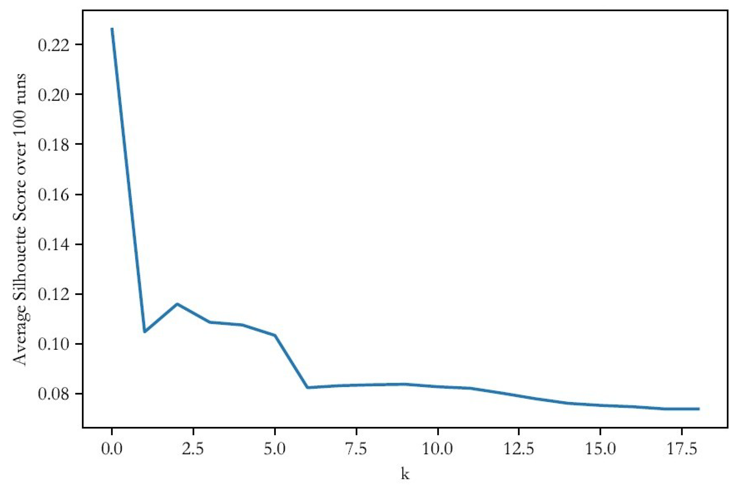
The number of clusters, k, was determined by an analysis of the average silhouette value, a measure of both cohesion and separation of clusters based on the difference between the average distance to points in the closest cluster and to points in the same cluster [35]. The silhouette analysis was also run 1000 times and an average silhouette score at each value of k was used to determine optimum k—see Figures 3 and 4.
In order to evaluate cluster stability, the Adjusted Rand Score was calculated to compare each run of the k-means algorithm to the run selected as the optimum cluster. This score computes a similarity measure between two clustering schemes by considering all of the pairs of samples and counting which pairs are in the same or different clusters [34]. It was used to evaluate whether k-means algorithm frequently converged to the same or a similar result, indicating the stability of the results.
Because a centroid was used as a proxy for the origin of all food buying trips within each block group, block groups that have a large area could potentially have a high margin of error with regard to their route distances. To see if this had a significant effect on the clustering scheme, distances were perturbed ten times by a function of an artificial radius for each block group, the k-means was recalculated, and the Adjusted Rand Score was used to compare the perturbed and centroid-based labeling schemes. Specifically:
with D the perturbed distance, d the original distance, r the artificial radius derived by treating each tract like a circle with r = sqrt(A/pi), with A the area of the circle encompassing the block group, and p the probability value between −1 and 1 selected using a random number generator following a normal distribution. The p variable was included to introduce stochasticity into the resulting distance, as an alternative to randomly resampling a point from each block group and using that to generate the route. The distances were perturbed using this function ten times. Ideally, this perturbation would have been conducted one hundred or one thousand times. However, due to computational constraints, ten perturbations were used to assess the validity of results.
D = d + (r × p)
4. Results and Discussion
To determine the optimal number of clusters, the silhouette analysis was run one thousand times for k = 2 through k = 20. Average values at each k for the thousand runs were calculated and plotted in Figure 3 and Figure 4, below. Based on the results of the silhouette analysis, k = 3 (silhouette score of 0.133) was selected for the rural set and k = 4 (average silhouette score of 0.115) was selected for the urban set. In both cases, silhouette scores at the chosen k spiked at these values and dropped for the remainder of the k-values.
According to the Adjusted Rand Score, the clustering solutions proved to be very stable with each simulation. For rural block groups, 985 of the 1000 runs had an Adjusted Rand Score of 0.9 or higher, meaning that 90% or more of the labels were in agreement with the optimum result’s labels. For the urban block groups, 391 of the 1000 cluster schemes were between 0.3 and 0.4, and 553 were above 0.9. Although this is less stable than the rural result, it still indicates that the k-means tended to converge to a labeling scheme similar to the one selected as the optimum result. The clustering solution after perturbing the distance calculations also showed an overall high agreement. The rural clusters were found to be more stable with respect to distance perturbation than the urban clusters. This was surprising because urban block groups are smaller, and therefore the radii being used to perturb the distance were smaller than the radii in rural block groups. The lower scores for urban block groups cluster validity may have been due to the comparative lack of stability in running k-means on the urban block groups. The high validity score for rural block groups where the total area from which people start their shopping trips is larger, is encouraging. The margin of error in these block groups was expected to be relatively high, and yet the clustering based on perturbed distances yielded 80% agreement with the clustering based on centroid distances. For the urban cases, the algorithm only produced a labeling scheme that matched the optimum result for half of the runs.
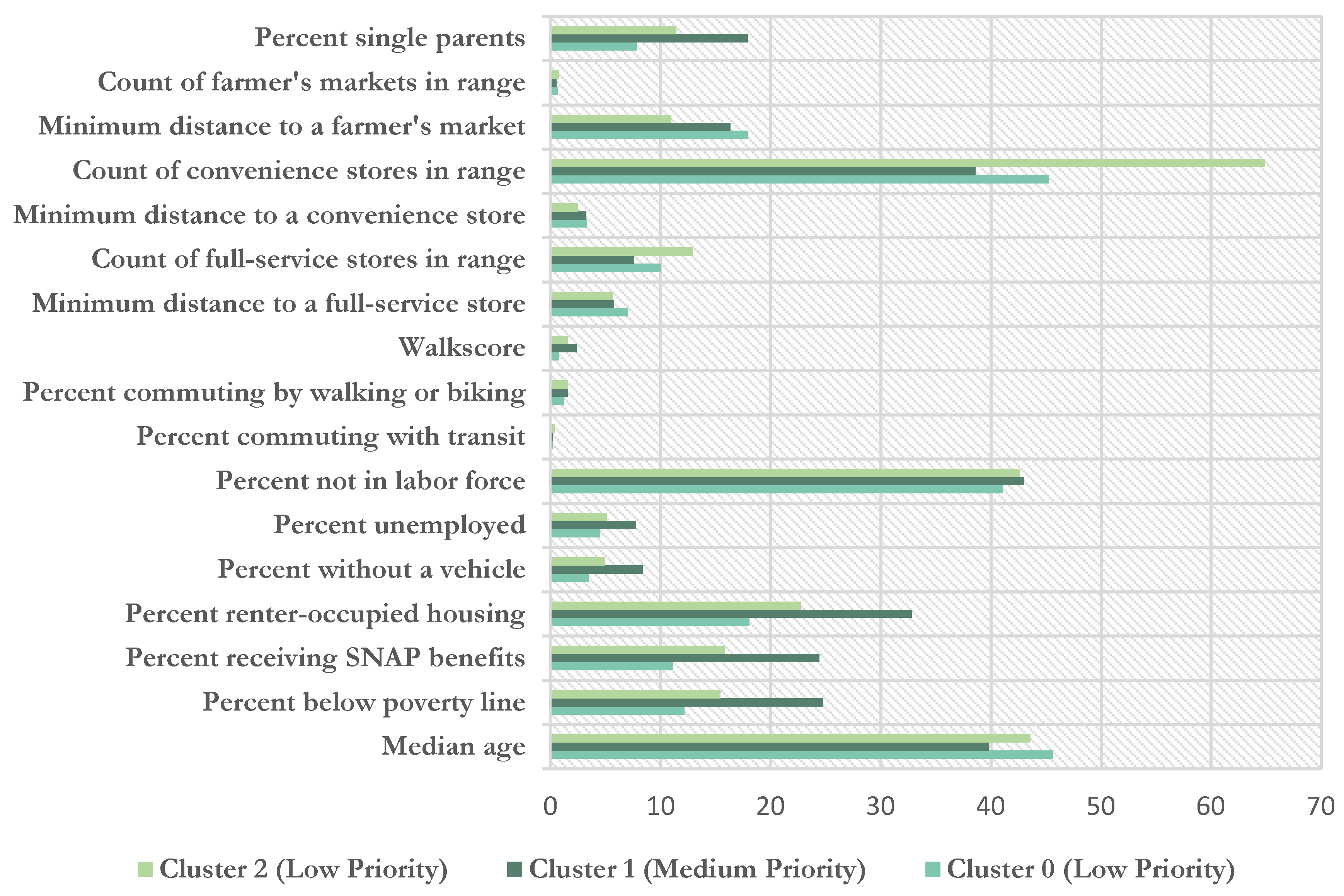
Descriptions of each of the groups are obtained by examining the distribution of each variable in each cluster. Summary statistics are visualized in Figure 5 and Figure 6, and summarized in Table 2 and Table 3. Based on the typical landscape in each group, a priority level was assigned (i.e., low/medium/high). Of the three rural groups, Cluster 1 was identified as the group most in need. It has the highest percentage of people below the poverty line, using SNAP benefits (24%), unemployed (7%), and without access to a vehicle (8%). Among households with children, approximately 18% are single parent households. The ratio of convenience stores to full services grocery stores is 5.1:1 and on average, the nearest grocery stores is 5.75 miles away. This group represents a middle range of values for all food access variables, but given the relatively large share of residents without access to a vehicle, the traditional 10-mile definition of food access would not apply. Overall, this group has the largest economic barrier to healthy food.
Clusters 0 and 2 are considered lower-priority groups for rural areas. Cluster 0 is the wealthiest with the lowest share of single parents, but they are on average farthest from a full-service grocery store or farmer’s market. Given the high share of residents with a car, a targeted strategy to improve access would be of lower priority than for other areas. Finally, Cluster 3 has middle range values for social and economic indicators, but the best access. Neighborhoods are generally not walkable, but 95% of residents have a car. Within 10 miles, this group has more both full-service (n = 12) and convenience stores (n = 64) in range. Of the 139 block groups included, only 1 did not have access to a full-service store in a 10-mile radius.
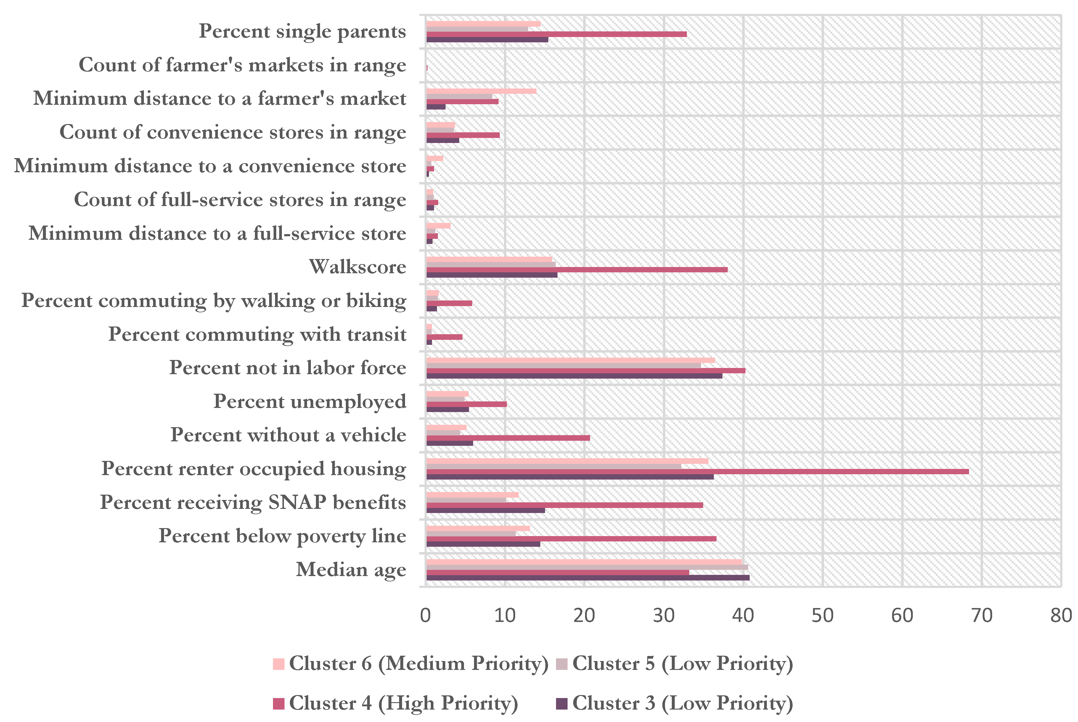
For the urban groups, Cluster 4 possesses the most precarious socioeconomic circumstances with the highest share of renters, poverty rates, SNAP participants, low car ownership and a relatively high share of transit riders and reliance on non-motorized transport. Neighborhoods are more walkable than any other group, but the closest grocery store is on average 1.5 miles away, 150% of the threshold distance allotted by the USDA for urban residents. A full 246 out of 961 block groups do not have access to a full-service store within this threshold distance. These neighborhoods have an overabundance of conveniences stores with a ratio of convenience to full-service stores close to 6:1 and are deemed the highest priority neighborhoods in urban areas for mitigation strategies. Neighborhoods belonging to this cluster would be ideal candidates for a number of place-based strategies that tackle the multidimensionality of their food access problems. They possess a trifecta of limitations covering transportation, poor socioeconomic conditions, and few food options that all need to be addressed in seeking a solution for these neighborhoods.
Of the remaining three urban clusters, Cluster 6 is identified as a medium priority group. These neighborhoods have average socioeconomic conditions, but are furthest from stores. They are on average 3.2 miles from a grocery store and 2.2 miles from a convenience stores with a ratio of convenience to full-service of 3:9. Almost exactly half do not have access to a full-service store within the 1-mile threshold suggested by the USDA. Therefore, while those in this group have high vehicle ownership rates and relatively high purchasing power, they would likely benefit from an increase in nearby food options.
The final two urban Clusters, 3 and 5, are deemed the lowest priority for place-based food access measures. Cluster 3 has the closest distances to food stores with an average minimum distance of 0.43 to convenience stores and 0.88 to full-service stores. The majority of the population has access to a private vehicle (94%) and as a group, their socioeconomic conditions are relatively high. Cluster 5 similarity has high car access, is primarily not using SNAP benefits (90%) and is largely employed (95%), suggesting that residents of these block groups have both the purchasing power and the transportation necessary to buy food on their own terms.
Cluster Mapping and Food Desert Comparison
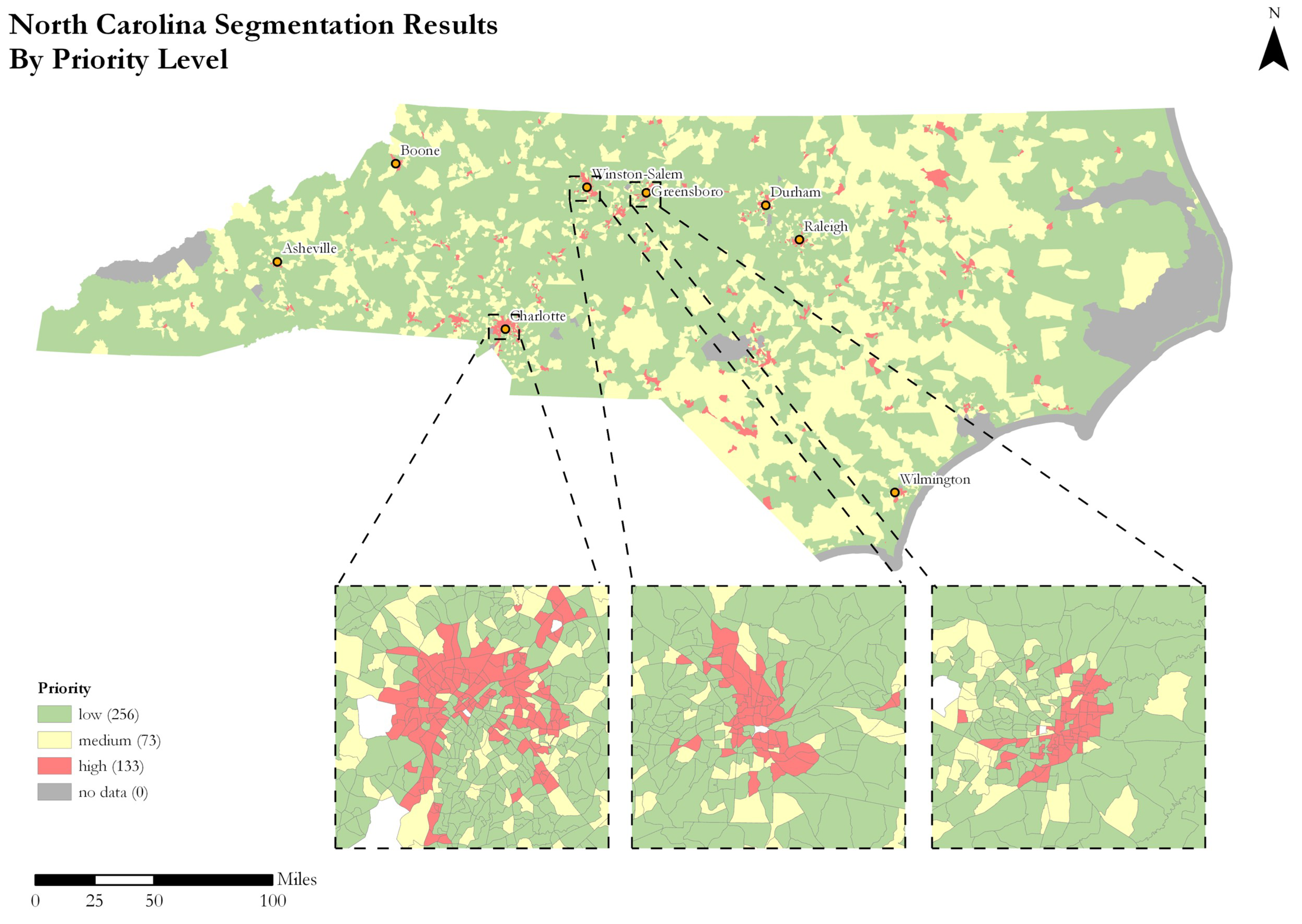
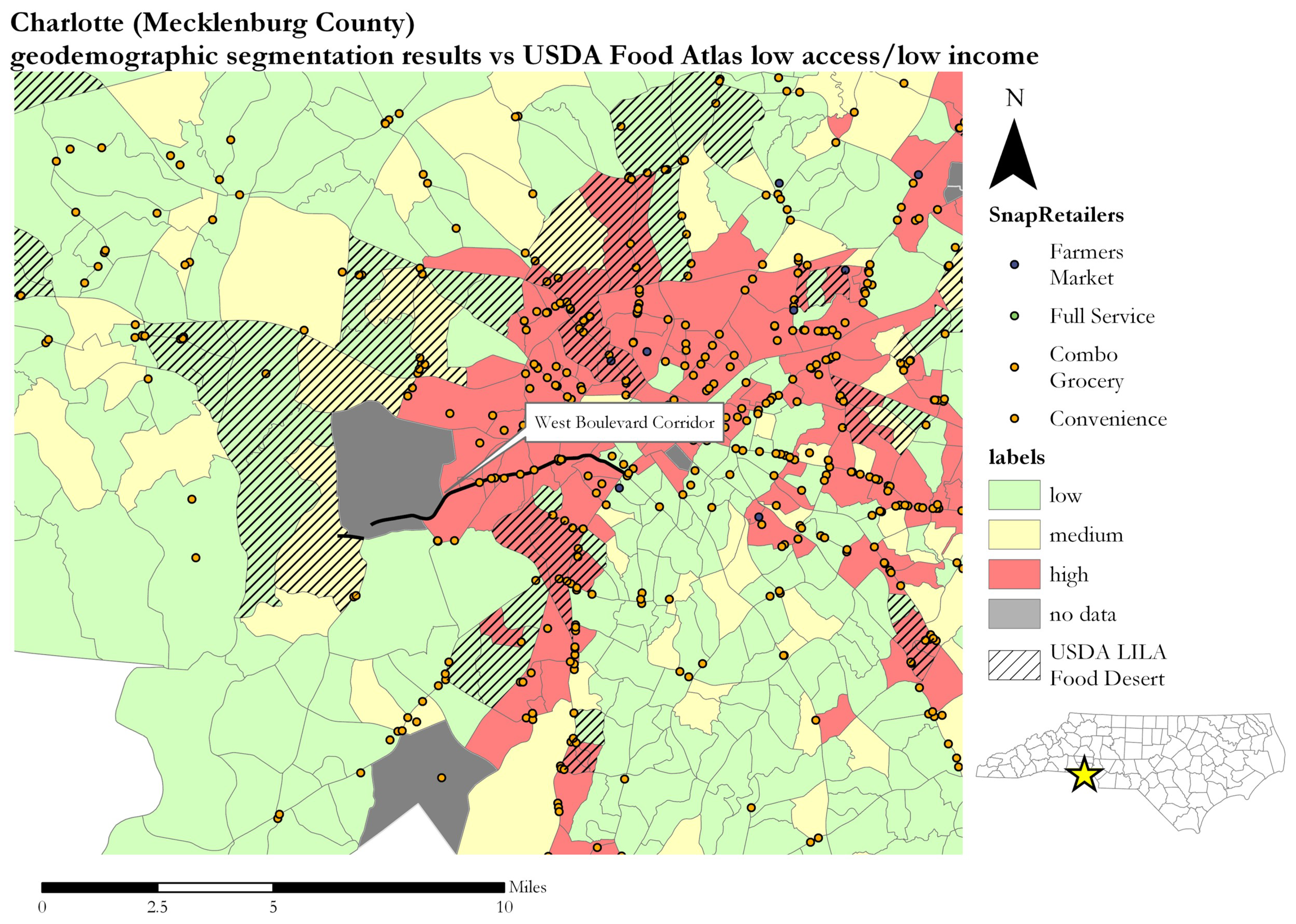
Figure 7 shows the spatial distribution of the seven classes throughout the state of North Carolina while Figure 8 shows this same area reclassified into the low/medium/high priority scale. The results are compared to the USDA’s low-income low-access measure at 1 mile urban/10 miles rural. The USDA releases census tracts that it considers to be food deserts as part of its Food Research Atlas. The result, showing Charlotte/Mecklenburg County, is shown in Figure 6. There is overlap between the food deserts and the high-priority cluster. However, in this case, the high-priority cluster also captures the West Boulevard Corridor, Charlotte’s most-cited food-insecure area [1] and the neighborhood where Tribonia Parker lives, which the USDA measures fail to highlight with their metric. This indicates that the high-priority group identified with this method serves its purpose in teasing out neighborhood areas that have limited access compounded with other factors that make purchasing healthy food difficult that are overlooked by the USDA’s approach.
To more fully compare our results with the USDA Food Atlas, we computed the percentage of overlap between our seven clusters and the four USDA categories: low income census tract where a significant share of residents is more than (1) 1 mile in an urban area or 10 miles in a rural area from the nearest supermarket; (2) a half mile in an urban area or 10 miles in an urban area; (3) 1 mile in an urban area or 20 miles in a rural area; and (4), where more than 100 housing units do not have a vehicle and are more than a half mile from the nearest supermarket in an urban area or a significant share of residents are more than 20 miles from the nearest supermarket in a rural area.
The USDA’s Food Atlas is published at the census tract level, a larger geographic unit compared to our census block group. The results do not perfectly map onto one another for comparison’s sake. We therefore computed the percentage of area overlap between our clusters and their groups as shown in Table 4 to gauge the compatibility of the two approaches. Overall, the highest amount of agreement is between our highest priority urban cluster and the USDA groups with nearly 40% overlap between the second USDA category and our urban high-priority cluster. As is evident in the map in Figure 9, however, our high-priority urban cluster is more encompassing that the USDA’s food desert tracts which are based on income and a single measurement of distance. Based on the anecdotal example provided above, such a simple definition of food insecurity does not capture the multidimensionality of the problem and hence our approach identifies a much larger area as having a restricted local food environment.
5. Conclusions
The purpose of this article was to implement a novel, place-based index for examining food access landscapes considering the multidimensionality of this issue. We adopted a geodemographic segmentation approach for categorizing the food access landscape that incorporated three distinct sources and categories of data: socioeconomic indicators from the American Community Survey of the US Census, distance measurements to grocery stores, farmer’s markets, and convenience stores, and a walkability index. A k-means clustering procedure was used to establish the segmentations, and ultimately seven different clusters—three rural, four urban—were identified throughout the state of North Carolina. The clusters were subsequently prioritized as high, medium, or low based on the characteristics of the variables associated with each group. The high-priority urban cluster, Cluster 4, had the greatest SNAP participation, the highest walkability, the highest percent without a car, and an average distance of one and a half miles to a full-service food store. Block groups in this cluster would be an ideal location to try to attract a supermarket, set up a community co-op or farmer’s market, or encourage urban gardening. Cluster 6 is also urban, considered medium priority, and had a much greater distance to food stores than all other urban clusters: an average of 3.2 miles to a convenience store. While most people have a car in these tracts, it would be ideal to improve transit connectivity or set up ridesharing for grocery trips to accommodate for those who do not have one or temporarily cannot use one. A similar solution might be helpful for rural Cluster 1, which was an average of 5.75 miles from a store and 10 percent of its population was without access to a car.
Overall, we found our highest priority cluster to be much more encompassing than the USDA food desert groups which are based on income and a single measure of grocery store distance. We were further able to tease out more specific policy recommendations when examining the problem from a more multidimensional perspective while also providing a prioritization for policy makers.
By embracing a contextual perspective on local food environments that considers the proximity and concentration of different types of stores, walkability, as well as various socioeconomic indicators, our approach overcomes some of the limitations that accompany a single variable strategy to defining food deserts, such as the USDA’s Food Desert Atlas. Our approach incorporates recent and publicly available datasets that make it replicable in other geographic areas. It also proved robust to alternative ways of measuring the average distance to stores from an aerial geographic unit. Clustering multiple attributes to paint a holistic portrait of the local food environment helps to de-emphasize the contribution of individual variables that may be error prone and thereby reduces the overall uncertainty of the results [32].
This paper has relied on several assumptions that may affect the validity of our approach. First, recent descriptive analyses of food deserts have placed an emphasis on incorporating the quality and pricing of food into determinations of access [11,12,18]. However, beyond differentiating between different types of stores, there is no estimation of food pricing or quality incorporated into this research. Perceived quality and price can create barriers to healthy foods in the same way that distance can, and this should be accounted for in future work. Second, this study would have benefitted from an estimation of transit coverage, to provide a better idea of how capable people without cars are of getting to a store with ease. Walk Score™ also has a Transit Score metric but only has data on a limited number of cities. Third, the demographic information used in this study is based on sample data from the ACS published in 2015. These samples are estimated based on a small number of answers from people living in the block group and although they are calculated to be representative, sampling bias is likely to play a role in the resulting values. Fourth, adding data on additional food programs would also help to make results both more realistic and more useful: SNAP is certainly the largest food assistance program in the United States, but it is by no means the only important one. The USDA’s Food and Nutrition Service has a number of other programs such as the Emergency Food Assistance Program (TEFAP) and the Food Distribution Program on Indian Reservations (FDPIR). Additionally, myriad state and local services also work to connect families with healthy food in a variety of ways, ranging from vouchers to food-growing co-ops. Moving toward more complete resources describing food programs would dramatically increase the effectiveness of research like that presented here. As a place-based metric, the idiosyncrasies of individuals such as daily space-time mobility patterns or food preferences were not incorporated, but could be an avenue for future improvement. Finally, further research on the validity of our results is warranted beyond the case study highlighted in this article. How well our results comport with real-world experiences of residents and their local food environment would provide additional validation to our analysis.
Our approach can help decision makers sort through the noise of small-area demographic and physical access data to find patterns on which they can base broad mitigation strategies. The results can also serve as a first step for investigation into regionally specific food access problems, highlighting potential problem areas for further investigation. Future implementations of food access geodemographic segmentations have the potential to improve upon these initial results and create more cohesive and impactful segmentations to use to guide planning and policy. However, the results presented in this North Carolina case study demonstrate a significant need for changes at a statewide level—over 900 block groups were found to be in the high-priority low-access group in cities throughout North Carolina. While these findings suggest the need for statewide oversight, they leave room for individual cities and counties to explore high-priority block groups and perhaps challenge their narrow conceptualizations of “food deserts” as determined by the USDA.
Author Contributions
Conceptualization, E.M.; Methodology, E.M., E.C.D. and E.D.; Formal Analysis, E.M.; Writing—Original Draft Preparation, E.M.; Writing—Review & Editing, E.M., E.C.D. and E.D.; Visualization, E.M., E.C.D. and E.D.; Supervision, E.C.D. and E.D.
Funding
This research received no external funding.
Conflicts of Interest
The authors declare no conflicts of interest.
References
- Peralta, K.; Off, G. Charlotte’s Grocery Wars Leave Poor Neighborhoods behind. The Charlotte Observer, 16 March 2017. Available online: https://www.charlotteobserver.com/news/business/article138771028.html (accessed on 28 April 2017).
- Raja, S.; Changxing, M.; Yadav, P. Beyond Food Deserts: Measuring and Mapping Racial Disparities in Neighborhood Food Environments. J. Plan. Educ. Res. 2008, 27, 469–482. [Google Scholar] [CrossRef]
- Richardson, A.S.; Meyer, K.A.; Howard, A.G.; Boone-Heinonen, J.; Popkin, B.M.; Evenson, K.R.; Kiefe, C.I.; Lewis, C.E.; Gordon-Larsen, P. Neighborhood Socioeconomic Status and Food Environment: A 20-Year Longitudinal Latent Class Analysis among CARDIA Participants. Health Place 2014, 11, 145–153. [Google Scholar] [CrossRef] [PubMed]
- USDA. Food Access Research Atlas. Available online: https://www.ers.usda.gov/data-products/food-access-research-atlas/ (accessed on 8 August 2018).
- Gallagher, M. USDA defines food deserts. Nutr. Dig. 2011, 38. Available online: http://americannutritionassociation.org/newsletter/usda-defines-food-deserts (accessed on 11 April 2017).
- Widener, M.J.; Farber, S.; Neutens, T.; Horner, M.W. Using Urban Commuting Data to Calculate a Spatiotemporal Accessibility Measure for Food Environment Studies. Health Place 2013, 21, 1–9. [Google Scholar] [CrossRef] [PubMed] [Green Version]
- Horner, M.W.; Wood, B.S. Capturing Individuals’ Food Environments Using Flexible Space-Time Accessibility Measures. Appl. Geogr. 2014, 51, 99–107. [Google Scholar] [CrossRef]
- Farber, S.; Morang, M.; Widener, M.J. Temporal Variability in Transit-Based Accessibility to Supermarkets. Appl. Geogr. 2014, 53, 149–159. [Google Scholar] [CrossRef]
- Widener, M.J.; Minaker, L.; Farber, S.; Allen, J.; Vitali, B.; Coleman, P.; Cook, B. How do changes in the daily food and transportation environments affect grocery store accessibility? Appl. Geogr. 2017, 83, 46–62. [Google Scholar] [CrossRef]
- Shannon, J.; Christian, W.J. What Is the Relationship between Food Shopping and Daily Mobility? A Relational Approach to Analysis of Food Access. GeoJournal 2017, 82, 769–785. [Google Scholar]
- LeClair, M.S.; Aksan, A.-M. Redefining the Food Desert: Combining GIS with Direct Observation to Measure Food Access. Agric. Hum. Values 2014, 31, 537–547. [Google Scholar]
- Mabli, J.; Worthington, J. The Food Access Environment and Food Purchase Behavior of SNAP Households. J. Hunger Environ. Nutr. 2015, 10, 132–149. [Google Scholar] [CrossRef]
- Ghirardelli, A.; Quinn, V.; Foerster, S. Using Geographic Information Systems and Local Food Store Data in Califorinia’s Low-Income Neighborhoods to Inform Community Initiatives and Resources. Am. J. Public Health 2010, 100, 2156–2162. [Google Scholar] [CrossRef] [PubMed]
- Bridle-Fitzpatrick, S. Food Deserts or Food Swamps?: A Mixed-Methods Study of Local Food Environments in a Mexican City. Soc. Sci. Med. 2015, 142, 202–213. [Google Scholar] [CrossRef] [PubMed]
- Andrews, M.; Smallwood, D. What’s Behind the Rise in SNAP Participation? Amber Waves 2012, 10, 1–6. [Google Scholar]
- Kaufman, P.R. Rural Poor Have Less Access to Supermarkets, Large Grocery Stores. Rural Dev. Perspect. 1999, 13, 19–26. [Google Scholar]
- Zenk, S.N.; Schulz, A.J.; Israel, B.A.; James, S.A.; Bao, S.; Wilson, M.L. Neighborhood Racia Composition, Neighborhood Poverty, and the Spatial Accessibility of Supermarkets in Metropolitan Detroit. Am. J. Public Health 2005, 95, 660–667. [Google Scholar] [CrossRef] [PubMed]
- Shannon, J. What Does SNAP Benefit Usage Tell Us about Food Access in Low-Income Neighborhoods? Soc. Sci. Med. 2014, 107, 89–99. [Google Scholar] [CrossRef] [PubMed]
- Racine, E.F.; Delmelle, E.; Major, E.; Solomon, C.A. Accessibility Landscapes of Supplemental Nutrition Assistance Program−Authorized Stores. J. Acad. Nutr. Diet. 2018, 118, 836–848. [Google Scholar] [CrossRef] [PubMed]
- Widener, M.J.; Li, W. Using Geolocated Twitter Data to Monitor the Prevalence of Healthy and Unhealthy Food References across the US. Appl. Geogr. 2014, 54, 189–197. [Google Scholar] [CrossRef]
- Kwan, M.P. Gender and individual access to urban opportunities: A study using space-time measures. Prof. Geogr. 1999, 51, 210–227. [Google Scholar] [CrossRef]
- Sleight, P. Targeting Customers: How to Use Geodemographic and Lifestyle Data in Your Business, 2nd ed.; NTC Publications: Henley-on-Thames, UK, 1997. [Google Scholar]
- Burrows, R.; Gane, N. Geodemographics, Software and Class. Sociology 2006, 40, 793–812. [Google Scholar] [CrossRef]
- Harris, R.; Sleight, P.; Webber, R. Geodemographics, GIS and Neighbourhood Targeting; John Wiley and Sons: Hoboken, NJ, USA, 2005. [Google Scholar]
- Dibb, S.; Simkin, L. Bridging the Segmentation Theory/Practice Divide. J. Mark. Manag. 2010, 25, 219–225. [Google Scholar] [CrossRef]
- Petersen, J.; Gibin, M.; Longley, P.; Mateos, P.; Atkinson, P.; Ashby, D. Geodemographics as a Tool for Targeting Neighbourhoods in Public Health Campaigns. J. Geogr. Syst. 2011, 13, 173–192. [Google Scholar] [CrossRef]
- Hamano, T.; Fujisawa, Y.; Ishida, Y.; Subramanian, S.V.; Kawachi, I.; Shiwaku, K. Social Capital and Mental Health in Japan: A Multilevel Analysis. PLoS ONE 2010, 5, e13214. [Google Scholar] [CrossRef] [PubMed]
- Grubesic, T.H.; Miller, J.; Murray, A.T. Geospatial and Geodemographic Insights for Diabetes in the United States. Appl. Geogr. 2014, 55, 117–126. [Google Scholar] [CrossRef]
- Delmelle, E.C. Five decades of neighborhood classifications and their transitions: A comparison of four US cities, 1970–2010. Appl. Geogr. 2015, 57, 1–11. [Google Scholar] [CrossRef]
- United States Census Bureau. American Community Survey. Available online: https://www.census.gov/programs-surveys/acs (accessed on 8 August 2018).
- Spielman, S.; Folch, D.; Nagle, N. Patterns and causes of uncertainty in the American Community Survey. Appl. Geogr. 2014, 46, 147–157. [Google Scholar] [CrossRef] [PubMed] [Green Version]
- Spielman, S.E.; Singleton, A. Studying neighborhoods using uncertain data from the American community survey: A contextual approach. Ann. Am. Assoc. Geogr. 2015, 105, 1003–1025. [Google Scholar] [CrossRef]
- Nanetti, L.; Cerliani, L.; Gazzola, V.; Renken, R.; Keysers, C. Group Analyses of Connectivity-Based Cortical Parcellation Using Repeated K-Means Clustering. NeuroImage 2009, 47, 1666–1677. [Google Scholar] [CrossRef] [PubMed]
- Skikit-learn. Scikit-learn-Machine Learning in Python. Available online: http://scikit-learn.org/stable/ (accessed on 8 August 2018).
- Zaki, M.J.; Meira, W., Jr.; Meira, W. Data Mining and Analysis: Fundamental Concepts and Algorithms; Cambridge University Press: Cambridge, UK, 2014. [Google Scholar]
Figure 1.
USDA’s Low Income/Low Access tracts (LILAs) in the Charlotte Mecklenburg area.

Figure 2.
Flowchart of Analytical Procedure.

Figure 3.
Average silhouette values for different values of k, rural block groups.

Figure 4.
Average silhouette values for different values of k, urban block groups.

Figure 5.
Average values of each variable belonging to the three rural clusters.

Figure 6.
Average values of each variable belonging to the four urban clusters.

Figure 7.
Spatial distribution of food access groups in North Carolina.

Figure 8.
Geodemographic groups reclassified into low, medium, and high-priority groups.

Figure 9.
Charlotte (Mecklenburg County) geodemographic segmentation results vs USDA Food Atlas low-access/low-income areas.
Figure 9.
Charlotte (Mecklenburg County) geodemographic segmentation results vs USDA Food Atlas low-access/low-income areas.


Table 1.
Variables used in geodemographic segmentation analysis.
| Variable Name | Source | Used in Final? | Description |
|---|---|---|---|
| MedAge | ACS 2015 (US Census Bureau, Washington DC, USA, 2015) | Yes | Median age of block group (of total pop.) |
| MedIncome | Yes | Median income of block group (of total households) | |
| PcHHBelowPov | Yes | Percent of households below the federal poverty line | |
| PcHH60plus | No | Percent of households with a person over age 60 | |
| PcSNAPHH | Yes | Percent of households receiving SNAP benefits | |
| PcSNAPHHdisability | No | Percent of households receiving SNAP with a disabled person | |
| PcHHrentocc | Yes | Percent of households who rent their homes | |
| PcHHNoVehicle | Yes | Percent of households who do not own a car | |
| PcWhite | No | Percent of total population that identifies as white | |
| PcBlack | No | Percent of total population that identifies as black | |
| PcHisp | No | Percent of total population that identifies as Hispanic | |
| PcAsian | No | Percent of total population that identifies as Asian | |
| PcNatAm | No | Percent of total population that identifies as Native American | |
| PcTwoRaces | No | Percent of total population who identify themselves as belonging to two races | |
| PcUnemploy | Yes | Percent of work eligible persons (over age 16) who are unemployed | |
| PcNotInLabor | Yes | Percent of work eligible persons (over age 16) who are not in the workforce | |
| PcCommuteCar | No | Percent of workers who commute by car | |
| PcCommuteCP | No | Percent of workers who commute in a carpool | |
| PcWalkBike | Yes | Percent of workers who walk or bike to their job | |
| PcTransit | Yes | Percent of workers who commute via public transit | |
| PcSingPar | Yes | Percent of households with children that are headed by a single parent of any gender | |
| Walkscore | Walk Score™ (Washington, USA, 2007) | Yes | Index describing walkability of neighborhoods, on a 0–100 scale |
| Min_mqdist_fs | MapQuest (Colorado, USA, 1967) | Yes | Minimum distance from block group’s population-weighted centroid to a full-service grocery store |
| Min_mqdist_concom | Yes | Minimum distance from block group’s population-weighted centroid to a convenience store or combo grocery | |
| Min_mqdist_fm | Yes | Minimum distance from block group’s population-weighted centroid to a farmer’s market | |
| Count_pp_fs | Yes | Total number of full-service stores within USDA food deserts range, divided by total pop. | |
| Count_pp_concom | Yes | Total number of convenience stores/combo groceries within USDA food desert range, divided by total pop. | |
| Count_pp_fm | Yes | Total number of farmer’s markets within USDA food desert range, divided by total pop. |
Table 2.
Average and standard deviation of variables belonging to three rural clusters.
| Variable | Metric | Cluster 0 n = 1238 | Cluster 1 n = 762 | Cluster 2 n = 139 |
|---|---|---|---|---|
| Median age | Average | 45.6222 | 39.7852 | 43.5741 |
| Standard Deviation | 7.1335 | 7.1066 | 7.4038 | |
| Percent below poverty line | Average | 12.1730 | 24.7355 | 15.4179 |
| Standard Deviation | 6.7422 | 9.0593 | 8.6482 | |
| Percent receiving SNAP benefits | Average | 11.1408 | 24.4011 | 15.8322 |
| Standard Deviation | 6.8400 | 10.1031 | 11.2097 | |
| Percent renter-occupied housing | Average | 18.0459 | 32.8212 | 22.7337 |
| Standard Deviation | 8.7674 | 11.1320 | 10.9185 | |
| Percent without a vehicle | Average | 3.5004 | 8.3587 | 4.9459 |
| Standard Deviation | 3.7080 | 6.5698 | 5.1283 | |
| Percent unemployed | Average | 4.4598 | 7.7809 | 5.1404 |
| Standard Deviation | 3.0318 | 4.7352 | 3.8901 | |
| Percent not in labor force | Average | 41.0416 | 42.9901 | 42.6050 |
| Standard Deviation | 10.0047 | 9.9739 | 10.2158 | |
| Percent commuting with transit | Average | 0.2047 | 0.2251 | 0.4108 |
| Standard Deviation | 0.9129 | 0.9991 | 2.0100 | |
| Percent commuting by walking or biking | Average | 1.2325 | 1.5924 | 1.6391 |
| Standard Deviation | 2.9092 | 3.3704 | 3.7216 | |
| Median income | Average | $44,229.78 | $41,258.28 | $40,265.20 |
| Standard Deviation | 24,712.32 | 20,285.45 | 14,684.70 | |
| Walkscore | Average | 0.8296 | 2.4108 | 1.5827 |
| Standard Deviation | 3.0493 | 7.3969 | 5.6897 | |
| Minimum distance to a full-service store | Average | 7.0337 | 5.7553 | 5.6433 |
| Standard Deviation | 4.7185 | 3.7983 | 3.0613 | |
| Count of full-service stores in range | Average | 9.9935 | 7.6024 | 12.8921 |
| Standard Deviation | 10.1896 | 7.5365 | 11.7036 | |
| Minimum distance to a convenience store | Average | 3.2766 | 3.2279 | 2.5184 |
| Standard Deviation | 2.4705 | 2.1410 | 1.5077 | |
| Count of convenience stores in range | Average | 45.2318 | 38.6076 | 64.8921 |
| Standard Deviation | 39.0225 | 31.7546 | 56.8120 | |
| Minimum distance to a farmer’s market | Average | 17.9316 | 16.3320 | 10.9763 |
| Standard Deviation | 12.3904 | 10.2971 | 5.8327 | |
| Count of farmer’s markets in range | Average | 0.7060 | 0.5801 | 0.7914 |
| Standard Deviation | 1.0645 | 0.8661 | 0.8689 | |
| Percent single parents | Average | 7.8368 | 17.9333 | 11.4207 |
| Standard Deviation | 6.2778 | 9.6056 | 9.0809 |
Table 3.
Average and standard deviation of variables belonging to four urban clusters.
| Variable | Metric | Cluster 3 n = 139 | Cluster 4 n = 961 | Cluster 5 n = 2083 | Cluster 6 n = 767 |
|---|---|---|---|---|---|
| Median age | Average | 40.7928 | 33.1637 | 40.5831 | 39.8280 |
| Standard Deviation | 8.2748 | 8.2138 | 8.4934 | 9.3201 | |
| Percent below poverty line | Average | 14.4240 | 36.6012 | 11.3437 | 13.1438 |
| Standard Deviation | 11.3427 | 14.4803 | 8.4311 | 9.6833 | |
| Percent receiving SNAP benefits | Average | 15.0163 | 34.9327 | 10.1078 | 11.6977 |
| Standard Deviation | 14.8804 | 16.8864 | 8.8113 | 10.3026 | |
| Percent renter-occupied housing | Average | 36.2608 | 68.3857 | 32.1779 | 35.5951 |
| Standard Deviation | 23.0801 | 17.0172 | 20.3527 | 22.3081 | |
| Percent without a vehicle | Average | 5.9877 | 20.7033 | 4.3440 | 5.1724 |
| Standard Deviation | 6.3230 | 13.1125 | 4.8434 | 5.9454 | |
| Percent unemployed | Average | 5.4701 | 10.2192 | 4.9098 | 5.4216 |
| Standard Deviation | 4.0155 | 6.4191 | 3.5562 | 3.8776 | |
| Percent not in labor force | Average | 37.3674 | 40.2774 | 34.6687 | 36.4324 |
| Standard Deviation | 11.3758 | 13.4624 | 11.2841 | 12.4056 | |
| Percent commuting with transit | Average | 0.8092 | 4.6457 | 0.7550 | 0.8128 |
| Standard Deviation | 2.2915 | 7.1180 | 2.0540 | 2.3157 | |
| Percent commuting by walking or biking | Average | 1.4185 | 5.8811 | 1.5386 | 1.6616 |
| Standard Deviation | 2.8334 | 9.5058 | 3.4404 | 3.8422 | |
| Median income | Average | $51,608.18 | $47,538.04 | $51,040.18 | $50,699.21 |
| Standard Deviation | 26,604.81 | 27,103.28 | 28,406.72 | 27,928.46 | |
| Walkscore | Average | 16.6043 | 38.0187 | 16.3874 | 15.9387 |
| Standard Deviation | 17.9698 | 20.1399 | 17.6144 | 16.6794 | |
| Minimum distance to a full-service store | Average | 0.8806 | 1.5394 | 1.2000 | 3.1583 |
| Standard Deviation | 0.5567 | 0.9583 | 0.5673 | 1.4061 | |
| Count of full-service stores in range | Average | 1.0504 | 1.5963 | 1.0307 | 0.9622 |
| Standard Deviation | 1.1526 | 1.9967 | 1.2877 | 1.5821 | |
| Minimum distance to a convenience store | Average | 0.4393 | 1.0421 | 0.7356 | 2.2044 |
| Standard Deviation | 0.2736 | 0.7551 | 0.3998 | 1.1596 | |
| Count of convenience stores in range | Average | 4.2230 | 9.3413 | 3.5607 | 3.7106 |
| Standard Deviation | 4.3083 | 6.0916 | 3.9686 | 5.6612 | |
| Minimum distance to a farmer’s market | Average | 2.4976 | 9.1647 | 8.3929 | 13.9345 |
| Standard Deviation | 4.6527 | 8.5506 | 7.8369 | 12.2955 | |
| Count of farmer’s markets in range | Average | 0.0504 | 0.2539 | 0.0696 | 0.0443 |
| Standard Deviation | 0.3246 | 0.5966 | 0.2947 | 0.2616 | |
| Percent single parents | Average | 15.4316 | 32.8695 | 12.9241 | 14.4575 |
| Standard Deviation | 11.8546 | 17.3353 | 10.2853 | 11.5918 |
Table 4.
Percentage overlap between four USDA food desert definitions and the seven clusters identified in this analysis.
Table 4.
Percentage overlap between four USDA food desert definitions and the seven clusters identified in this analysis.
| Cluster Label | Classification | Priority Level | Total Area (mi2) | Area Overlap in mi2 (%) | |||
|---|---|---|---|---|---|---|---|
| LILA at 1 mi Urban, 10 mi Rural | LILA at 0.5 mi Urban, 10 mi Rural | LILA at 1 mi Urban, 20 mi Rural | LILA with Vehicle Access at 20 mi | ||||
| 0 | Rural | Low | 24,873.3 | 248.6 (1.0%) | 248.6 (1.0%) | 72.3 (0.3%) | 482.4 (1.94%) |
| 1 | Rural | Medium | 14,808.4 | 244.5 (1.7%) | 244.5 (1.7%) | 84.9 (0.6%) | 824.0 (5.56%) |
| 2 | Rural | Low | 2490.1 | 21.5 (0.9%) | 21.5 (0.9%) | 13.5 (0.5%) | 78.8 (3.2%) |
| 3 | Urban | Low | 255.4 | 20.6 (8.1%) | 29.4 (11.5%) | 20.6 (8.1%) | 21.4 (8.4%) |
| 4 | Urban | High | 913.9 | 199.5 (21.8%) | 350.2 (38.3%) | 199.5 (21.8%) | 295.6 (32.3%) |
| 5 | Urban | Low | 4607.6 | 281.0 (6.1%) | 365.6 (7.9%) | 281.0 (6.1%) | 234.1 (5.1%) |
| 6 | Urban | Medium | 1773.6 | 234.1 (13.2%) | 158.5 (8.9%) | 234.1 (13.2%) | 103.8 (5.9%) |
© 2018 by the authors. Licensee MDPI, Basel, Switzerland. This article is an open access article distributed under the terms and conditions of the Creative Commons Attribution (CC BY) license (http://creativecommons.org/licenses/by/4.0/).
Share and Cite
MDPI and ACS Style
Major, E.; Delmelle, E.C.; Delmelle, E. SNAPScapes: Using Geodemographic Segmentation to Classify the Food Access Landscape. Urban Sci. 2018, 2, 71. https://doi.org/10.3390/urbansci2030071
AMA Style
Major E, Delmelle EC, Delmelle E. SNAPScapes: Using Geodemographic Segmentation to Classify the Food Access Landscape. Urban Science. 2018; 2(3):71. https://doi.org/10.3390/urbansci2030071
Chicago/Turabian StyleMajor, Elizabeth, Elizabeth C. Delmelle, and Eric Delmelle. 2018. "SNAPScapes: Using Geodemographic Segmentation to Classify the Food Access Landscape" Urban Science 2, no. 3: 71. https://doi.org/10.3390/urbansci2030071