Observational Constraints on Dynamical Dark Energy with Pivoting Redshift


1
Department of Physics, Liaoning Normal University, Dalian 116029, China
2
Department of Mathematics, Presidency University, 86/1 College Street, Kolkata 700073, India
3
Jodrell Bank Center for Astrophysics, School of Physics and Astronomy, University of Manchester, Oxford Road, Manchester M13 9PL, UK
4
Department of Physics, National Technical University of Athens, Zografou Campus, GR 157 73 Athens, Greece
5
Department of Astronomy, School of Physical Sciences, University of Science and Technology of China, Hefei 230026, China
6
National Observatory of Athens, Lofos Nymfon, 11852 Athens, Greece
*
Author to whom correspondence should be addressed.
Universe 2019, 5(11), 219; https://doi.org/10.3390/universe5110219
Submission received: 6 September 2019
/
Revised: 24 October 2019
/
Accepted: 13 November 2019
/
Published: 16 November 2019
(This article belongs to the Special Issue Probing the Dark Universe with Theory and Observations)
Abstract
:We investigate the generalized Chevallier–Polarski–Linder (CPL) parametrization, which contains the pivoting redshift as an extra free parameter, in order to examine whether the evolution of the dark energy equation of state can be better described by a different parametrization. We use various data combinations from cosmic microwave background (CMB), baryon acoustic oscillations (BAO), redshift space distortion (RSD), weak lensing (WL), joint light curve analysis (JLA), and cosmic chronometers (CC), and we include a Gaussian prior on the Hubble constant value, in order to extract the observational constraints on various quantities. For the case of free we find that for all data combinations it always remains unconstrained, and there is a degeneracy with the value of the dark energy equation of state at . For the case where is fixed to specific values, and for the full data combination, we find that with increasing the mean value of slowly moves into the phantom regime, however the cosmological constant is always allowed within 1 confidence-level. In fact, the significant effect is that with increasing , the correlations between and (the free parameter of the dark energy equation of state quantifying its evolution with redshift), change from negative to positive, with the case corresponding to no correlation. The fact that the two parameters describing the dark energy equation of state are uncorrelated for justifies why a non-zero pivoting redshift needs to be taken into account.
1. Introduction
According to observational evidences from various sources it has been established that our universe entered a dark energy-dominated era and began a period of accelerated expansion roughly billion years ago [1]. In order to provide an explanation, physicists follow two main directions. The first is to maintain general relativity as the gravitational theory and introduce new, exotic fluids in the universe content, dubbed as the dark energy sector [2,3]. The second way is to modify the gravitational sector, constructing extended theories of gravity that possess general relativity as a particular limit, but which, in general, present extra degrees of freedom, capable of describing the universe behavior [4,5,6,7,8].
However, both approaches can be quantified by the introduction of an equation-of-state parameter for the dark energy perfect fluid (effective in the case of modified gravity), namely , where , are respectively the pressure and the energy density. Hence, introducing various parametrizations of allows us to describe the universe evolution in a phenomenological way, even if the microphysical origin of the cause of acceleration is unknown. Following this, a large number of parametrizations have been introduced in recent years, namely the one-parameter dark energy parametrizations [9,10], or the two-parameter family, such as the Chevallier–Polarski–Linder (CPL) parametrization [11,12], the Linear parametrization [13,14,15], the Logarithmic parametrization [16], the Jassal–Bagla–Padmanabhan parametrization (JBP) [17], the Barboza–Alcaniz (BA) parametrization [18], etc. (see for instance [19,20,21,22,23,24,25,26,27,28,29,30,31,32,33,34,35,36,37,38,39,40,41,42,43,44,45,46,47] and the references therein).
In most of the above dark energy equation-of-state parametrizations with a two-parameter description, one sets the “pivoting redshift” to zero, namely the point in which the two parameters describing are uncorrelated. However, due to possible rotational correlations between the two parameters of the two-parameter models, in principle one could avoid setting the pivoting redshift to zero straightaway, and let it as a free parameter [48,49,50].
In the present work we are interested in investigating the observational constraints on the most well-known parametrization, namely the CPL one, incorporating however the pivoting redshift as an extra parameter, assuming it to be either fixed or free. The motivation of this choice is to examine if the evolution of the dark energy equation of state can be better described by introducing more freedom in this parametrization. A first examination towards this direction was performed in [51], however in the present work we provide a robust analysis with the latest cosmological data. In particular, we will use data from cosmic microwave background (CMB), baryon acoustic oscillations (BAO), redshift space distortion (RSD), weak lensing (WL), joint light curve analysis (JLA), and cosmic chronometers (CC), while we will include a Gaussian prior on the Hubble constant value. Among all the datasets mentioned above, some are related to the background evolution, such as JLA and CC, while CMB data play a very important role concerning the information of the model at the level of perturbations.
The plan of the work is as follows: In Section 2 we present the basic equations of a parametrized dark energy model at the background and perturbative levels. Section 3 describes the various data sets used in this work. In Section 4 we perform the observational confrontation, extracting the constraints on the model parameters and on various cosmological quantities. In Section 5 we proceed to a comparison of the various generalized CPL parametrization, with and without pivoting redshift. Finally, we summarize the obtained results in Section 6.
2. Dynamical Dark Energy with Pivoting Redshift
In this section we briefly review the basic equations for a non-interacting cosmological scenario both at background and perturbative levels, and we introduce the pivoting redshift dark energy parametrization. We consider the homogeneous and isotropic Friedmann–Lemaître–Robertson–Walker (FLRW) line element
where is the scale factor and corresponds to open, closed, and flat geometry, respectively. Additionally, we consider that the universe is filled with baryons, cold dark matter, radiation, and the (effective) dark energy fluid. Hence, the evolution of the universe is determined by the Friedmann equations, which are written as
where G is Newton’s gravitational constant and is the Hubble function, with dots denoting derivatives with respect to the cosmic time t. Moreover, in the above equations we have introduced the total energy density and pressure of the universe, reading as and , with the symbols corresponding to radiation, baryon, cold dark matter, and dark energy fluid, respectively. In the following we focus our analysis on the spatially flat case (), which is the one favored by observations.
In the case where the above sectors do not present mutual interactions, we can write the conservation equation of each fluid as
where is known as the equation-of-state parameter of the i-th fluid (). For radiation, , for baryons , for cold dark matter , and is time dependent in general. Thus, using the conservation Equation (4), one could easily extract that , , , where () is the present value of (). In the case of the dark energy fluid, the solution of (4) is
where is the current value of and is the value of the scale factor today which is set to unity by definition. Thus, inserting the evolution laws of the different components of the universe, one can explicitly express the Hubble function (2) as:
From the expression (5) one can deduce that the evolution of the dark energy component is highly dependent on the form of its equation-of-state parameter . In the simplest case where the dark energy fluid evolves as . Nevertheless, for dynamical one may consider various parametrizations in terms of the scale factor or the redshift z, where . Thus, in the literature one can find many forms of such parametrizations.
One of the well known parametrizations of the dark energy equation-of-state parameter is the Chevallier–Polarski–Linder (CPL) one, given by [11,12]
where is the current value of and at . One can see that the CPL parametrization can be generalized by introducing a new parameter in the following way [48,49,50]
where , and . The parameter describes the dark energy equation-of-state at . In the case where the extra parameter , we obtain , and thus we recover the standard CPL model (7). The parameter is called the “pivoting redshift” or decorrelation redshift with its corresponding scale factor, and indicates the point in which the two parameters describing , i.e., and , are uncorrelated, minimizing the error on . Essentially, marks the point in which is most tightly constrained, given the data [48,49,50]. We note that the pivot redshift is chosen in such a way so that the parameters and become uncorrelated. In particular, it is known that in the above parametrization , and thus , depend on the probing method, the fiducial scenario, and the imposed priors [48]. Hence, in principle one could avoid setting straightaway, and let it as a free parameter. Thus, can be more precisely determined than , and actually it is indeed the most precisely determined value of . In this work we are interested in investigating the generalized CPL parametrization (8), namely incorporating the pivoting redshift as an extra parameter, assuming it to be either fixed or free.
We proceed by providing the cosmological equations at the perturbation level. In the synchronous gauge the perturbed FLRW metric reads as
where is the unperturbed and the perturbed metric, and is the conformal time. Using the above perturbed metric one can solve the conservation equations . Thus, for a mode with wavenumber k the perturbed equations can be written as [52,53,54]
where primes denote derivatives with respect to the conformal time, and is the conformal Hubble factor. Additionally, is the density perturbation for the i-th fluid, is the divergence of the i-th fluid velocity, is the trace of the metric perturbations , and is the anisotropic stress of the i-th fluid. Note that in the following we set for all i, since we assume zero anisotropic stress for all fluids. If we denote the sound speed of the i-th fluid by , then it is given by the relation and the adiabatic speed of sound of the i-th fluid is given by , which is related to the equation of state as . For barotropic fluids, and in addition if constant, then . Now, for the dark energy fluid with equation of state , if it is assumed to be purely adiabatic, then , that means we have an imaginary value of and hence there appear instabilities in the perturbations. To fix this problem, it is necessary to impose and it is natural to set by hand [55].
3. Observational Data
In this section we present the various observational data sets that are going to be used in order to confront dark energy parametrizations with pivoting redshift. In our analysis we incorporate the data by varying nine cosmological parameters: the baryon energy density (where is the actual baryon density and is the critical density1 of the universe), the cold dark matter energy density , the reionization optical depth , the spectral index of the scalar perturbations , the logarithm of the amplitude of the primordial power spectrum , the ratio between the sound horizon and the angular diameter distance at decoupling , the two free parameters of the extended CPL parametrization (8), namely, and , and the pivot redshift . Furthermore, we explore all parameters within the range of the conservative flat priors shown in Table 1.
Let us now present in detail the data sets that we will use.
- Cosmic microwave background (CMB): We constrain the parameters by analyzing the full range of the 2015 Planck temperature and polarization power spectra () [56,57]. This dataset is identified as the Planck TTTEEE + lowTEB. At the time of writing only the Planck 2015 likelihood was publicly available, however we do not expect the conclusions of this paper to change significantly given the similarities between the Planck 2015 and Planck 2018 results [58,59].
- Baryon acoustic oscillations (BAO): We consider the baryon acoustic oscillations as was done in [60]. They are the 6 dF Galaxy Survey (6dFGS) measurement at [61], the Main Galaxy Sample of Data Release 7 of Sloan Digital Sky Survey (SDSS-MGS) at [62], and the CMASS and LOWZ samples from the Data Release 12 (DR12) of the Baryon Oscillation Spectroscopic Survey (BOSS) at and at [63].
- Redshift space distortion (RSD): We add two redshift space distortion data. In particular, we include the data from CMASS and LowZ galaxy samples. The CMASS sample consists of 777,202 galaxies having the effective redshift of [64], whereas the LOWZ sample consists of 361,762 galaxies having an effective redshift of [64].
- Joint light curve analysis (JLA): We consider the joint light curve analysis sample [68] consisting of 740 luminosity distance measurements of Supernovae Type Ia data in the redshift interval .
- Cosmic chronometers (CC): We add the thirty measurements of the cosmic chronometers in the redshift interval . The CC data have been summarized in [69].
- We include a Gaussian prior on the Hubble constant value from Riess et al. [70] (i.e., ), referred to as HST.
In order to incorporate statistically the several combinations of datasets and extract the observational constraints, we use our modified version of the publicly available Monte Carlo Markov Chain package Cosmomc [71], which is an efficient Monte Carlo algorithm equipped with a convergence diagnostic based on the Gelman and Rubin statistic [72]. It implements an efficient sampling of the posterior distribution using the fast/slow parameter decorrelations [73] and additionally it includes the support for the Planck data release 2015 Likelihood Code [57]2.
4. Observational Constraints
In this section we provide the observational constraints on the generalized CPL parametrization with pivoting redshift. We consider two separate cosmological scenarios, namely one where the pivoting redshift is handled as a free parameter, and one where we fix the pivoting redshift to specific values in the region . Moreover, in order to acquire a complete picture of the behavior of the scenario, we consider different combinations of the observational datasets described above.
4.1. Pivoting Redshift as a Free Parameter
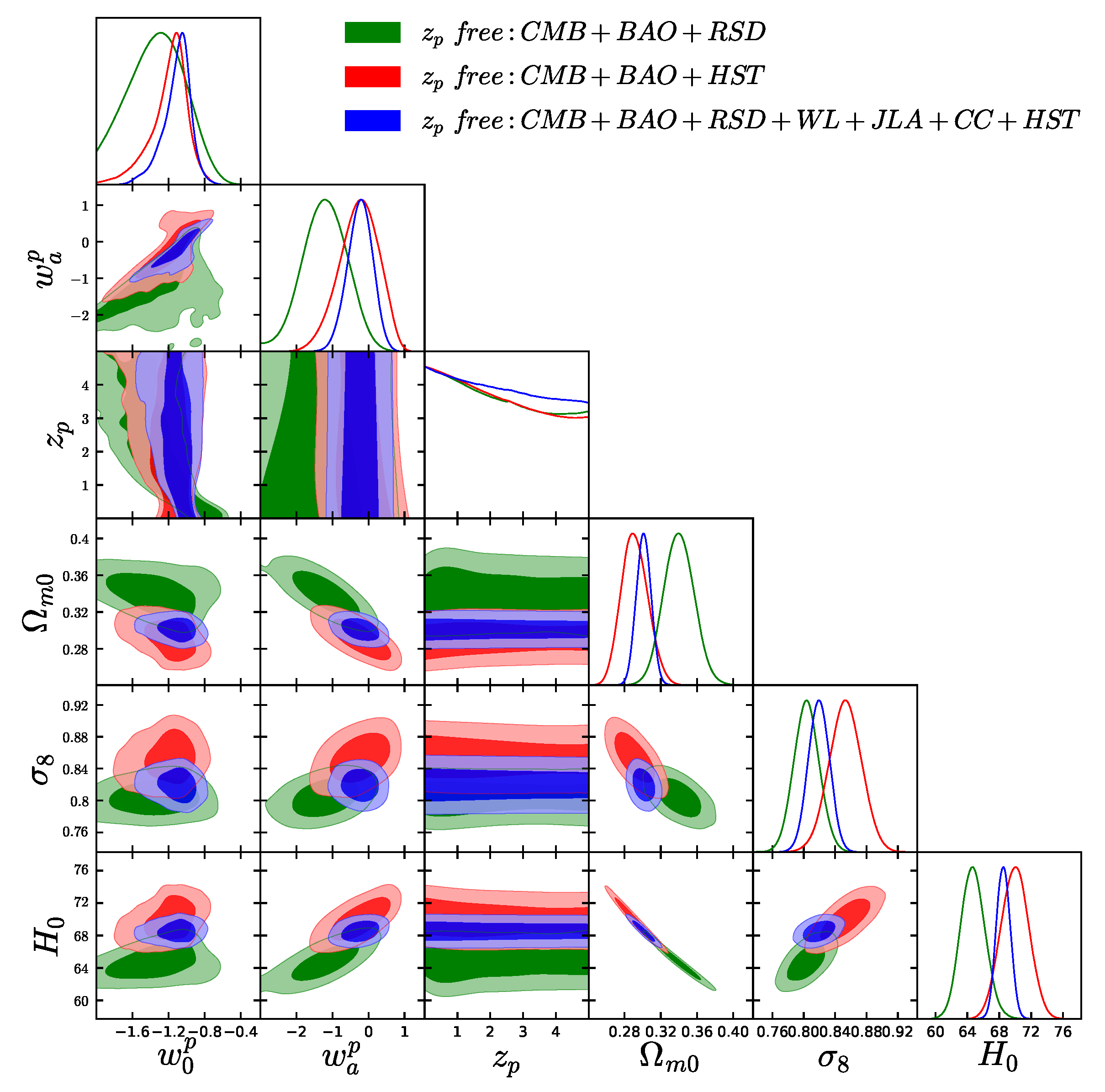
We desire to impose observational constraints on the generalized CPL parametrization (8), handling the pivoting redshift as a free parameter. The results of the analysis can be seen in Table 2, where we display the 68% (1) confidence level (CL) constraints for various quantities, while the full contour plots are presented in Figure 1.
For the case where only CMB data are used, the Hubble constant value at present increases and its error bars are strikingly large ( at 68% CL). Moreover, the dark energy equation-of-state parameter for this free is found to lie deeply in the phantom region, with at 68% CL.
When the BAO and RSD data are added to CMB (shown in Table 2 as the CBR combination), decreases ( at 68% CL) as well as its error bar, while the matter density increases significantly ( (at 68% CL). Additionally, in this data combination we obtain changes in the dark energy constraints. In particular, although the mean value of the dark energy equation-of-state parameter for free is in the phantom regime at 68% CL, however, the quintessence regime is allowed too, in contrast to the constraints from CMB only.
When the BAO and the HST data are added to CMB (i.e., the combined analysis CMB + BAO + HST called CBH in Table 2), the value of increases again. Concerning we also see that a phantom mean value is favored, nevertheless the quintessence regime is allowed within 1. In addition, the parameter increases significantly in comparison to its CMB and CMB + BAO + RSD constraints. However, as can be seen in Figure 1, note that the contour plots of the combination of CMB + BAO + RSD data (green contours) are in tension with CMB + BAO + HST ones (red contours).
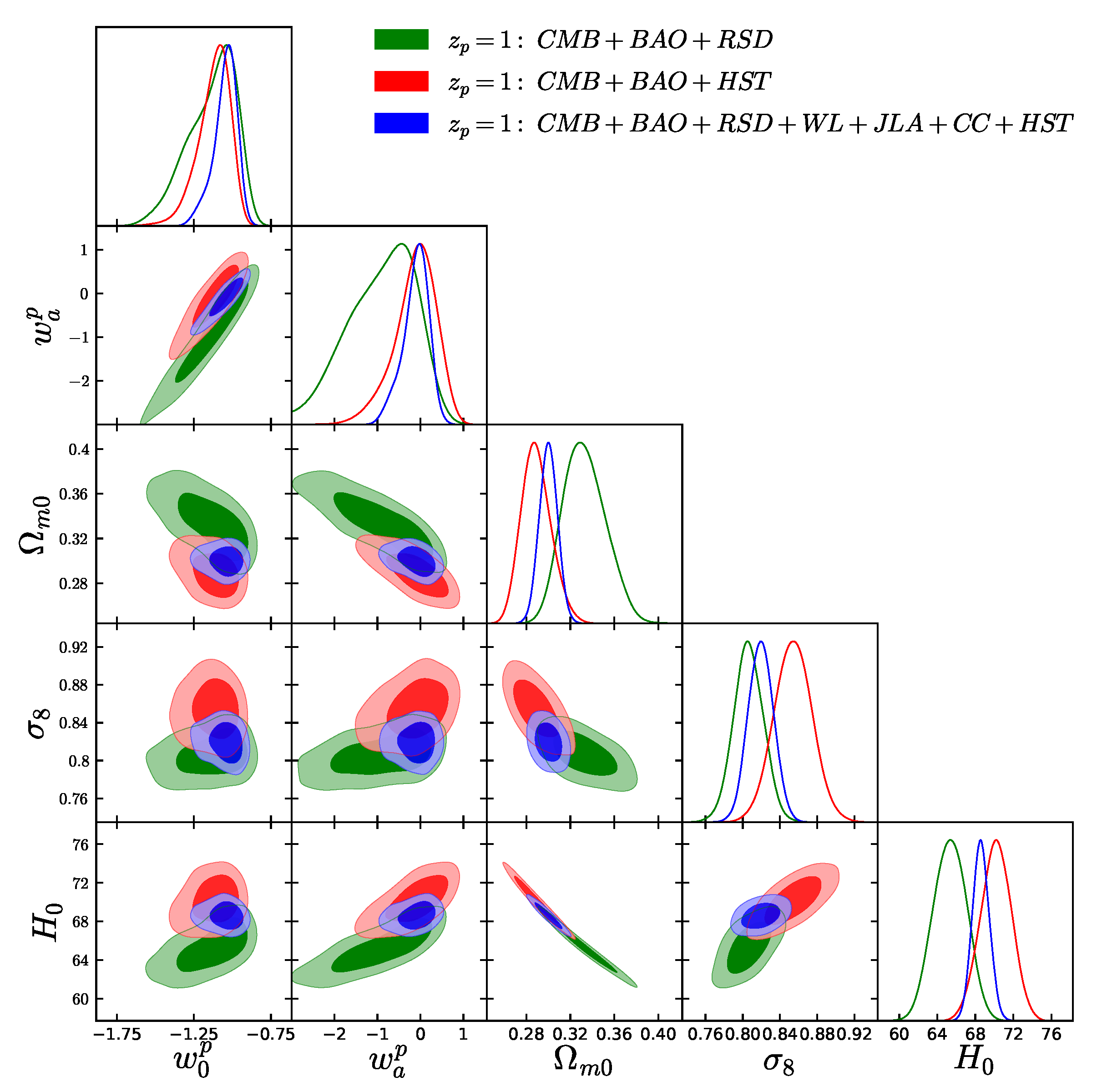
Finally, for the full analysis with all data sets (i.e., CMB + BAO + RSD + WL + JLA + CC + HST named collectively as CBRWJCH), summarized in the last column of Table 2, we find that the error bars on decrease compared to the other three analyses. Furthermore, the value of is in agreement with the cosmological constant within , which can also be seen in Figure 1.
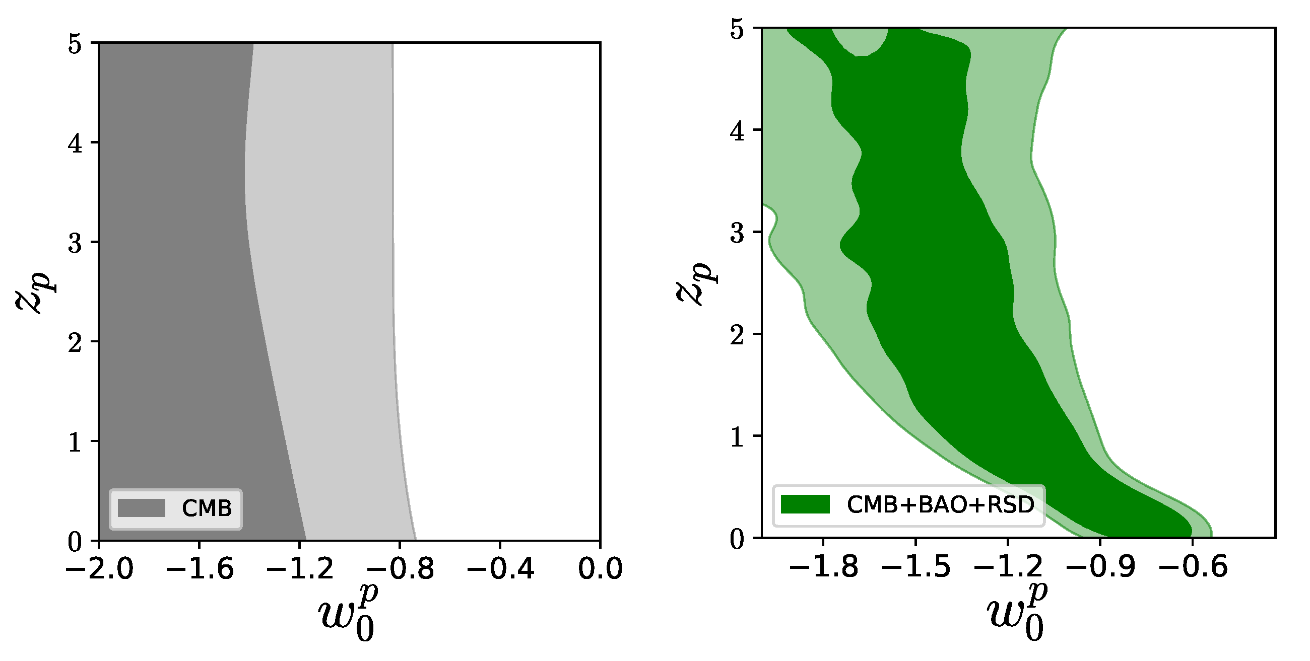
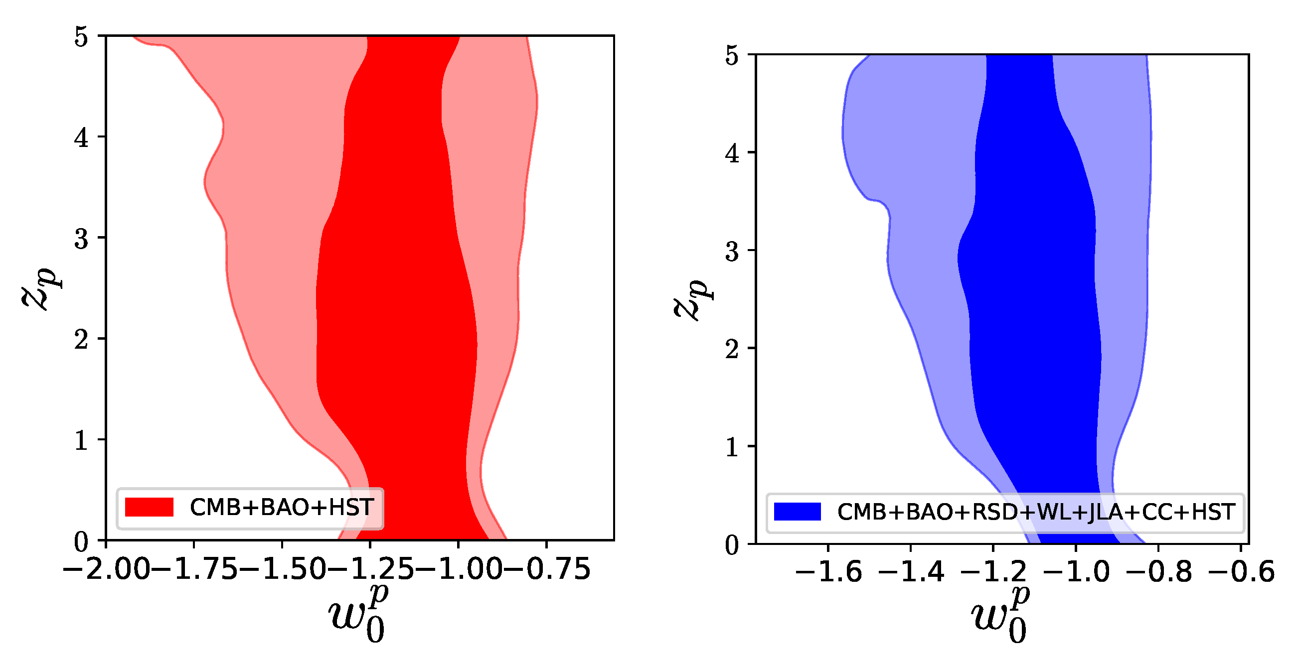
As we observe, for all combinations of data used, the pivoting redshift remains unconstrained in the range , since remains uncorrelated with most of the cosmological parameters, with the exception of the current dark energy equation of state . In order to provide the latter behavior in a clearer way in Figure 2 we present the corresponding contour plots in the plane. Hence, it is of great importance to examine the cosmological constraints on the generalized CPL model, handling as a fixed parameter, but still with a value different than which is its standard CPL value. This is performed in the next subsection.
4.2. Fixed Pivoting Redshifts
In this subsection we proceed to the investigation of the generalized CPL parametrization (8), handling as a fixed parameter in the range . In particular, we consider six different values of , namely , and 1, in order to examine how the observational constraints will change. Moreover, to be uniform we consider the same data combinations with the previous subsection.
4.2.1. Pivoting Redshift
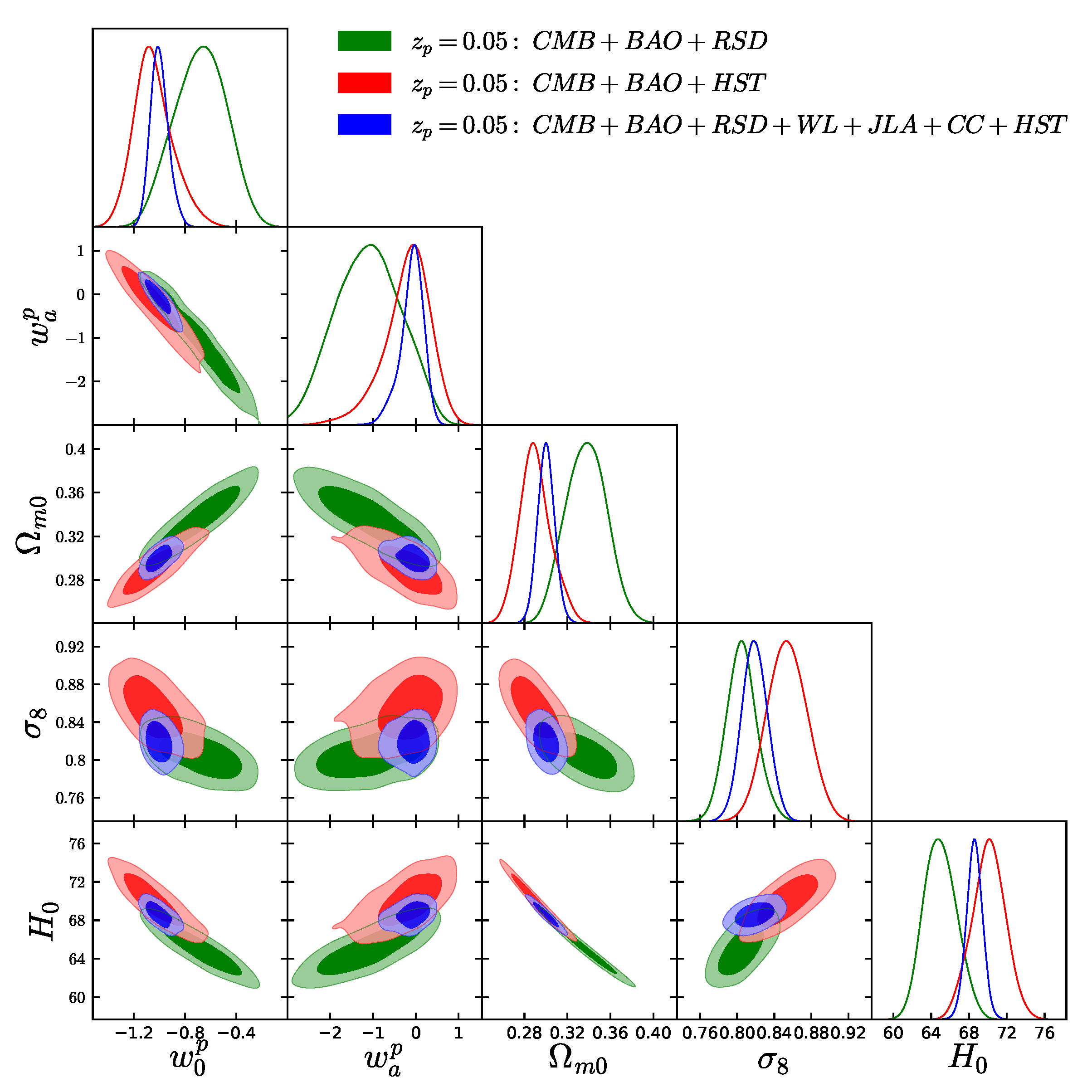
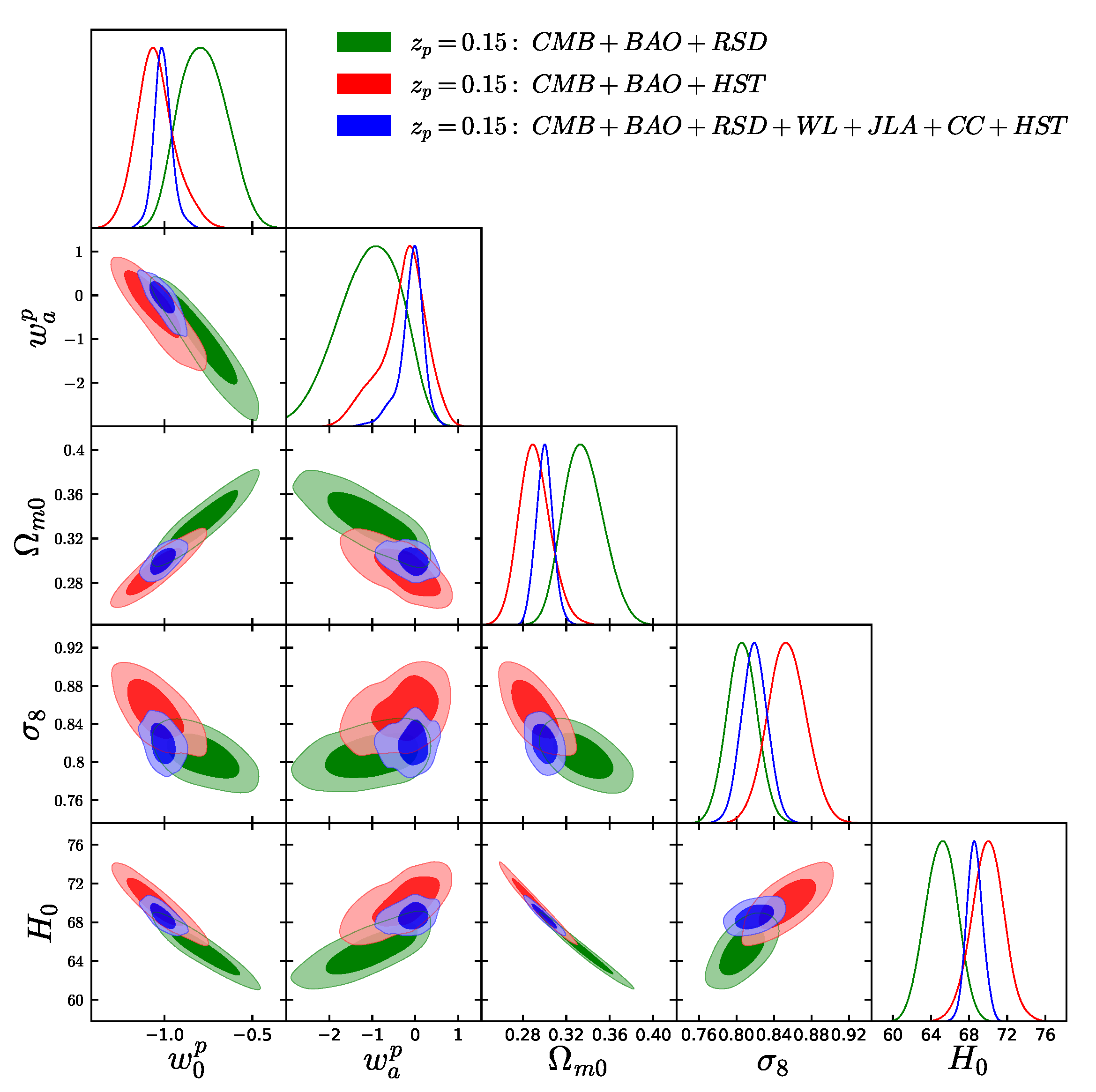
We begin our analysis choosing a very small value and we perform the observational fittings considering several data combinations. The results are summarized in Table 3 and the 68% and 95% CL contour plots are displayed in Figure 3.
In the case where we use the CMB data only, the current Hubble constant acquires a large value (at 68% CL), with significantly large error bars. Concerning the dark energy equation-of-state parameter at this pivoting redshift, that means where , its mean value lies in the phantom regime ( at 68% CL), nevertheless it is consistent with the cosmological constant within one standard deviation.
In the case where we include BAO and RSD to CMB data (this combination is named as CBR in Table 3) we obtain lower values ( at 68% CL) and its error bars are significantly reduced. Moreover, lies in the quintessence regime in more than 1 ( at 68% CL), however (or ) appears to be different from zero at more than one standard deviation ( at 68% CL), due to its strong anti-correlation with . Finally, for this data combination the matter density parameter at present is rather large ( at 68% CL) compared to the Planck 2015 results [64].
On the other hand, including BAO and HST to CMB data (this combination is denoted as CBH in Table 3) decreases with respect to the sole CMB case ( at 68% CL), but it acquires a higher value with respect to the dataset CBR, in a similar way to what we observed in the free analysis presented in Section 4.1. Additionally, is in agreement with the cosmological constant value at 68% CL, while the parameters and are in better agreement with the Planck 2015 findings comparing to the previous data combination CBR above.
Finally, the full combined analysis CMB + BAO + RSD + WL + JLA + CC + HST produces stronger constraints on the parameters, and the results are in significantly better agreement with CDM cosmology. Concerning the dark energy equation-of-state parameter at this particular pivoting redshift we obtain and at 68% CL. These values clearly show that for such low value of the pivoting redshift , the value of is extremely close to that of the cosmological constant boundary and in addition the strength of is decreased.
4.2.2. Pivoting Redshift
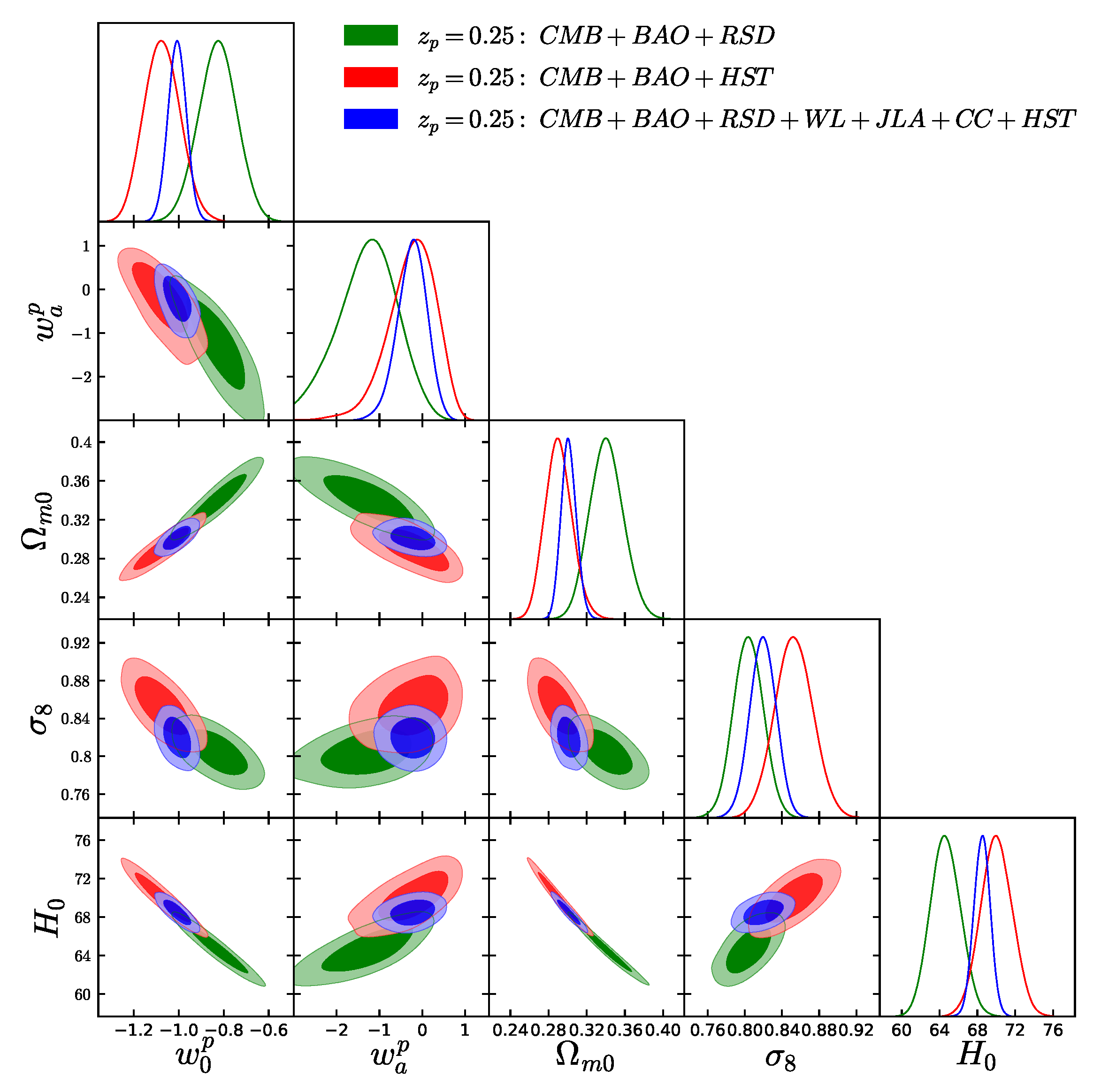
We proceed to the case where the pivot redshift is fixed to a slightly larger value, namely . The results of the observational confrontation for various datasets are summarized in Table 4, and the 68% and 95% CL contour plots are presented in Figure 4.
For the case of CMB data only the increased , comparing to the analysis of the previous paragraph, leads to smaller values ( at 68% CL). On the other hand, and increase in comparison to the previous, , analysis.
In the combined analysis CMB + BAO + RSD we also see that is slightly shifted towards the cosmological constant comparing to the case. Furthermore, for the last two combinations of datasets, namely, CMB + BAO + HST (CBH in Table 4) and the full CMB + BAO + RSD + WL + JLA + CC + HST (CBRWJCH in Table 4) we find that the observational constraints are very similar to those obtained for the case with .
4.2.3. Pivoting Redshift
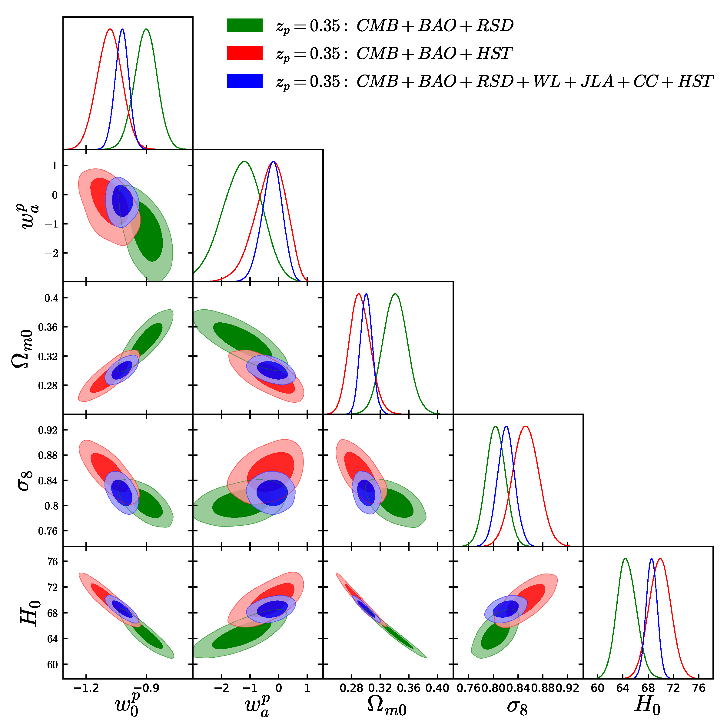
We fix the pivoting redshift to and in Table 5 we summarize the fitting results, while in Figure 5 we present the corresponding 68% and 95% CL contour plots.
For the case of CMB data only, is very similar to that obtained for the analysis with . However, at more than 68% CL, while in the previous analyses with and we had found at 1. Additionally, concerning we observe that its mean value lies in the middle between the value obtained for and .
When we add external data sets to CMB we find significant improvements in the estimations of the Hubble parameter, and its error bars are one order of magnitude smaller. The pattern of the analysis for the combined dataset CMB + BAO + RSD remains the same as the previous two analyses with the pivoting redshifts and . In fact, is in the quintessential regime at more than one standard deviation, and the matter density parameter shifts towards higher values. A significant improvement appears when we consider the two combinations of data sets, namely, CMB + BAO + HST and CMB + BAO + RSD + WL + JLA + CC + HST, where the various quantities exhibit similar trends with the previous two fixed pivoting redshifts. We mention that the two key parameters of the dark energy parametrization, namely and , are now in perfect agreement with the cosmological constant.
4.2.4. Pivoting Redshift
We now consider a slightly higher pivot redshift value, namely , and we summarize the fitting results in Table 6, while in Figure 6 we show the corresponding 68% and 95% CL contour plots.
The observational pattern for this parametrization is the same as the previous cases. We find that the CMB data only constrain at more than 68% CL, and we recover the cosmological constant scenario as soon as we add more external datasets to CMB. In this case, it appears an indication for at one standard deviation also for the CMB + BAO + HST case. Moreover, the results with the full combination of datasets are very stable and robust towards changing the fixed pivot redshift.
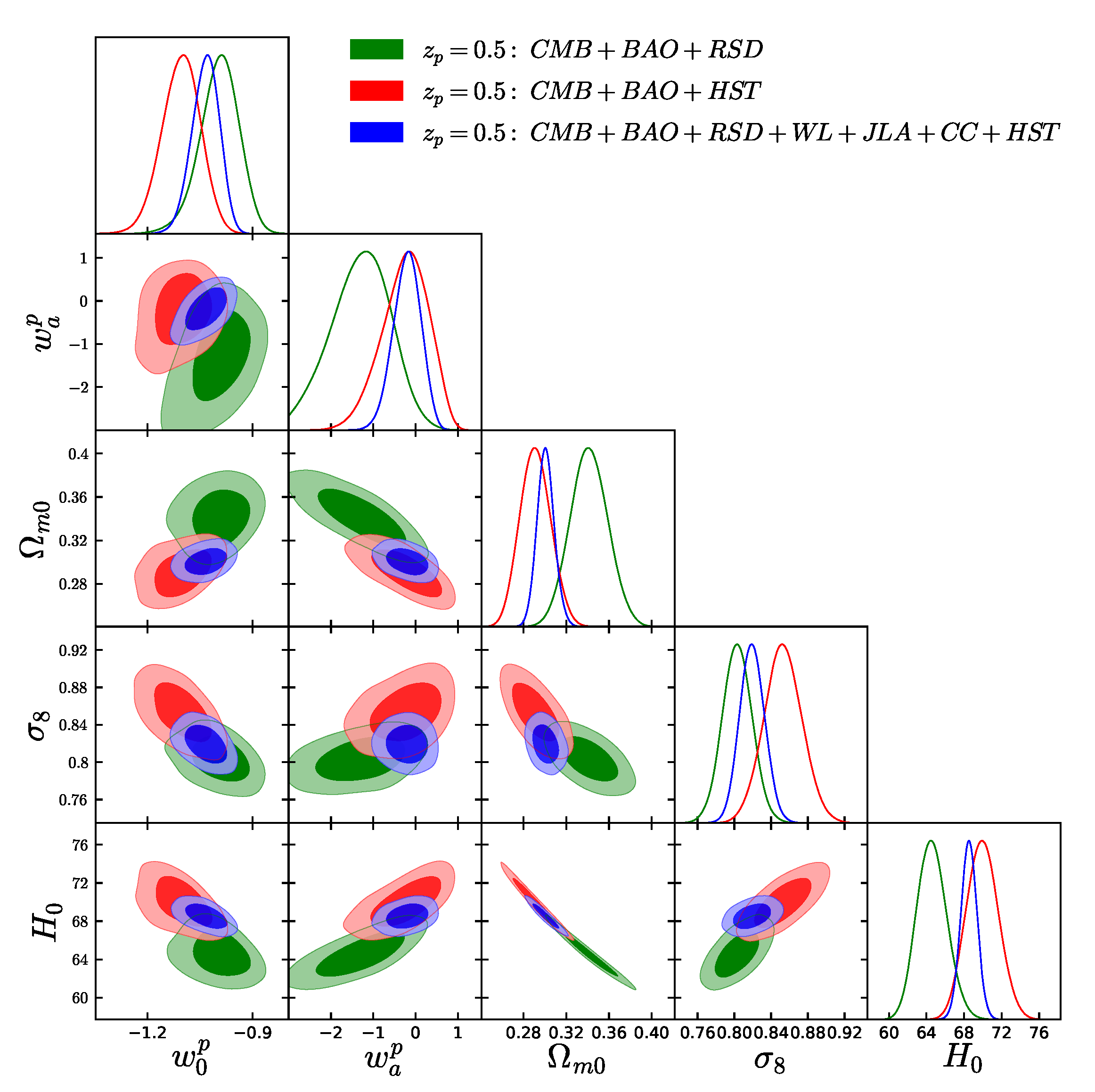
4.2.5. Pivoting Redshift
For the case , we summarize the fitting results in Table 7 and in Figure 7 we present the corresponding 68% and 95% CL contour plots. As we see, the constraints on the parameters are very similar to the case . In particular, we have the preference for a phantom regime at one standard deviation for the CMB and the CMB + BAO + HST cases, while on the other hand for the combinations CMB + BAO + RSD and CMB + BAO + RSD + WL + JLA + CC + HST the parametrization is in agreement with the cosmological constant.
4.2.6. Pivoting Redshift
Finally, we consider the last fixed pivoting redshift in this series, namely . In Table 8 we summarize the fitting results while in Figure 8 we depict the corresponding 68% and 95% CL contour plots. The overall results are similar with respect to the previous fixed pivot redshift cases, however, one can clearly see that for CMB + BAO + RSD data sets has a mean value in the phantom regime ( at 68% CL). Therefore, with the increment of the pivoting redshift we find a successive change in the estimation of . One can further notice that for the CMB data only is always favored, but all the other combinations of data recover the cosmological constant within 68% CL.
5. Statistical Comparison of All Parametrizations
In this section we proceed to a comparison of the various generalized CPL parametrizations, with and without the pivoting redshift. Hence, for completeness we perform a similar observational confrontation with the previous section for the standard CPL parametrization, namely without pivoting redshift (i.e., ), and we summarize the results in Table 9.
We can now perform the model comparison following the summarizing tables given above, namely Table 2 (varying ), Table 3 (), Table 4 (), Table 5 (), Table 6 (), Table 7 (), Table 8 (), and Table 9 (no pivoting redshift, i.e., ).
First of all, from all the analyses we find that the CMB data alone do not provide stringent constraints on the free parameters, however, we observe that the addition of any external datasets leads to a refinement of the constraints by reducing their error bars in a significant way. Furthermore, we find that the CMB + BAO + RSD combination returns slightly different constraints compared to the remaining two datasets, nevertheless for this combination we find an interesting pattern in the parameter, where we observe that with increasing , eventually approaches towards the cosmological constant value and finally for large () it crosses the boundary. Concerning the remaining two datasets, namely CMB + BAO + HST and CMB + BAO + RSD + WL + JLA + CC + HST, we find that the cosmological constraints are similar, with the best constraints definitely achieved for the final combination. Thus, in this section we focus on the observational datasets CMB + BAO + RSD and CMB + BAO + RSD + WL + JLA + CC + HST, in order to provide a statistical comparison between the cosmological models for free and fixed pivoting redshift .
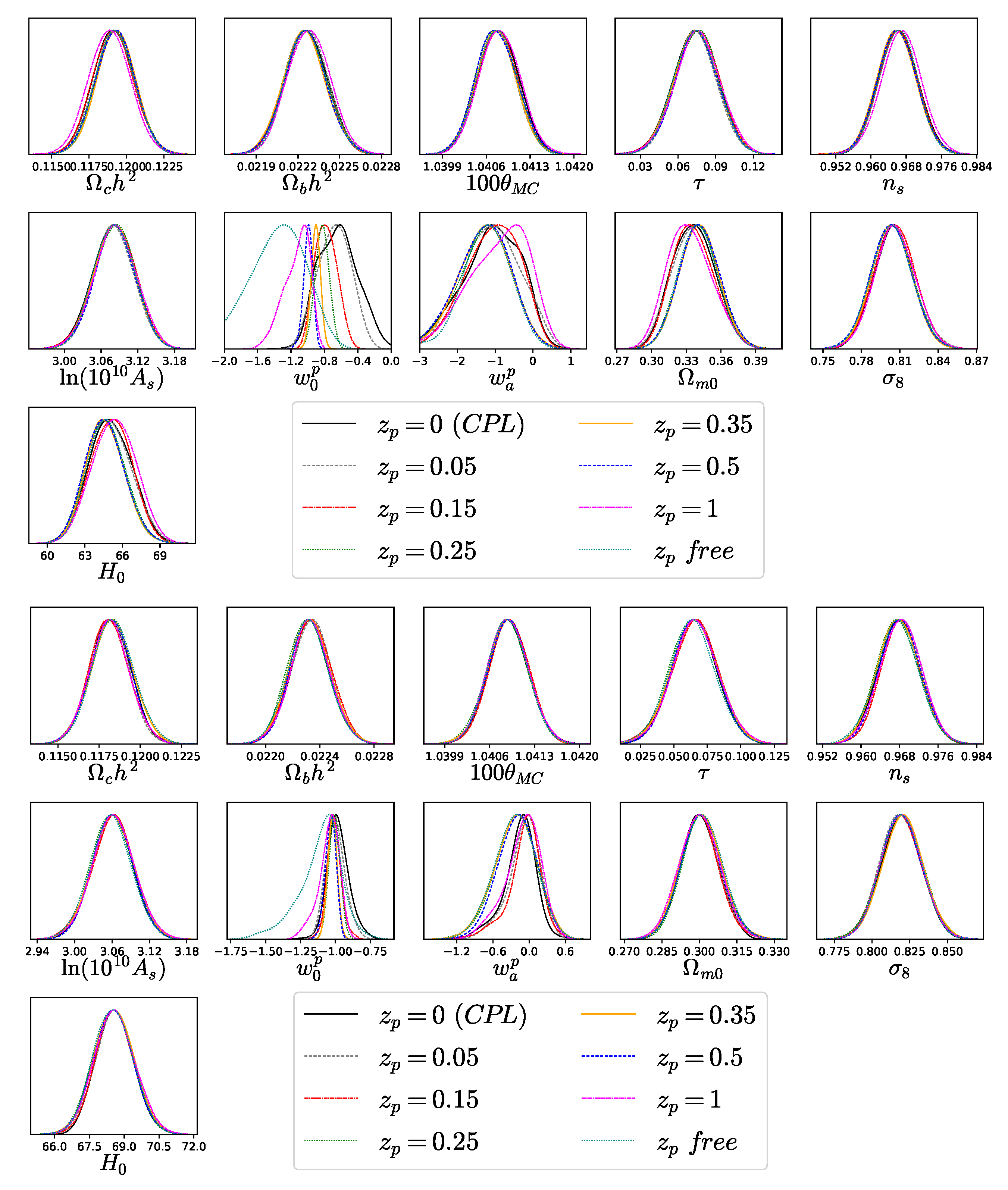
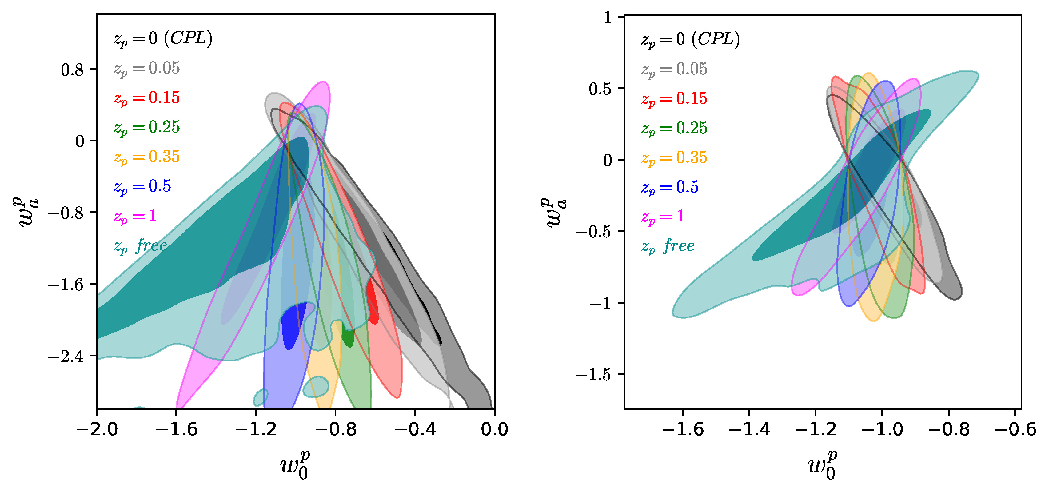
In order to proceed towards the statistical comparisons of the models, in Table 10 we depict the constraints on the basic model parameters for different values of (free and fixed). Furthermore, in Figure 9 we present the one-dimensional marginalized posterior distributions for the free parameters. In particular, the upper part of Figure 9 corresponds to the CMB + BAO + RSD dataset, while the lower part to the full combination CMB + BAO + RSD + WL + JLA + CC + HST. From both parts of Figure 9 we can clearly notice that all parameters present the same behavior independently of the pivoting redshift , apart from and . Hence, in order to examine in more detail the effect of on , , in Figure 10 we depict the contour plots in the plane for various , for the combinations CMB + BAO + RSD (left panel of Figure 10) and CMB + BAO + RSD + WL + JLA + CC + HST (right panel of Figure 10).
As we observe in Figure 10 for both datasets, by changing the values of the correlations between and change significantly. In particular, starting from a negative correlation present for (the original CPL parametrization), increasing the values leads to a rotation of the direction of the degeneracy between these two parameters. Therefore, we find a positive correlation for , as well as in the case where is left free. Finally, we can identify the value of the pivoting redshift for which and are no more correlated, and this is approximately for both datasets (the contours corresponding to (yellow) are vertical, showing no degeneracy). The changing of the correlations from negative to positive is one of the main results of this work.
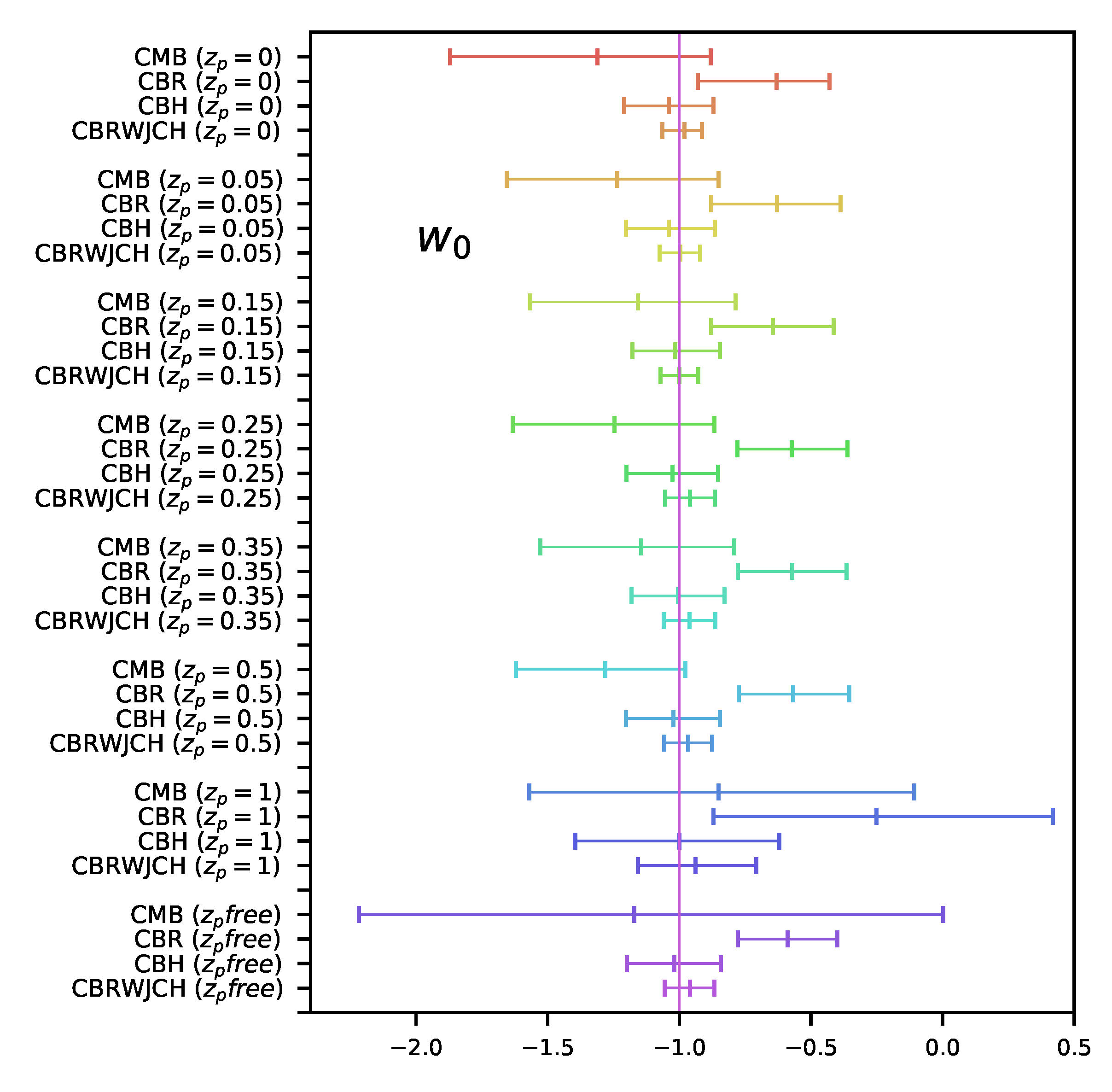
Lastly, in order to provide the obtained results in a more transparent way, in Figure 11 we provide the whisker plot for the equation-of-state parameter at present, namely , for all the examined cases of the generalized CPL parametrization (see Table 11 for the numerical values of at 68% CL that we have extracted using the values of , through , and the corresponding pivot redshift).
6. Concluding Remarks
Dynamical dark energy parametrizations are an effective approach to understanding the evolution of the universe, without needing to know the microphysical origin of the dark energy and whether it corresponds to new fields or to gravitational modification. Hence, a large number of such dark energy equation-of-state parametrizations have been introduced in the literature, with the Chevallier–Polarski–Linder (CPL) being one of the most studied.
However, in most of the above two-parameter parametrizations one considers the “pivoting redshift” to correspond to zero, namely the point in which the two parameters describing are uncorrelated, minimizing the error on this. Due to possible rotational correlations between the two parameters, in principle one could avoid setting the pivoting redshift to zero straightaway, handling it as a free parameter.
In the present work we investigated the observational constraints on such a generalized CPL parametrization, namely incorporating the pivoting redshift as an extra parameter, assuming it to be either fixed or free. For this, we used various data combinations from cosmic microwave background (CMB), baryon acoustic oscillations (BAO), redshift space distortion (RSD), weak lensing (WL), joint light curve analysis (JLA), and cosmic chronometers (CC), and we additionally included a Gaussian prior on the Hubble constant value. We considered two different cases, namely one in which is handled as a free parameter, and one in which it is fixed to a specific value. For the later case we considered various values of , in order to examine how the fixed value affects the results.
For the case of free , we found that for all data combinations always remains unconstrained, and there is a degeneracy with the dark energy equation of state (see Figure 2). On the other hand, in the case where is fixed we did not find any degeneracy in the parameter space, as expected. In particular, the mean values of lie always in the phantom regime, and for higher values of (), at more than 1 while for lower values of () the quintessence regime is also allowed at 1.
The inclusion of any external data set to sole CMB data, such as BAO + RSD, BAO + HST, and BAO + RSD + WL + JLA + CC + HST, significantly improves the CMB constraints by reducing the error bars on the various quantities. For instance, irrespectively of the different fixed values, the CMB data always return high values for the present Hubble constant with large error bars, which both decrease for the combined data cases.
Concerning the constraints on , for the CMB + BAO + RSD dataset we saw that they depend on the values of . In particular, for low () the mean values of are always quintessential, while for the mean value of lies in the phantom regime. Nevertheless, a common characteristic is that for all values is allowed within 68% CL (note that for within 68% CL is strictly greater than ). Furthermore, for the CMB + BAO + HST dataset we saw that the obtained -values for different are in better agreement with the cosmological constant. Additionally, for the last full combination of CMB + BAO + RSD + WL + JLA + CC + HST, we also found that is consistent with the cosmological constant, independently of the values. As expected, compared to all the analyses performed in this work, the cosmological constraints obtained for the full data combination, namely CMB + BAO + RSD + WL + JLA + CC + HST, are much more stringent, as it was summarized in the whisker plot of Figure 11.
Finally, in the above analysis we were able to reveal a correlation between the parameters and for different (see Figure 10). In particular, we found that with increasing the correlations between and change from negative to positive (the direction of degeneracy is rotating from negative to positive), and for the case , and are uncorrelated. Hence, has a special interest because for this particular value of the redshift the aforementioned parameters become uncorrelated. This is one of the main results of the present work. Since the pivoting redshift is defined as the point in which and are considered uncorrelated, and having found that this is not true for but for indeed justifies why a non-zero pivoting redshift needs to be taken into account.
Author Contributions
W.Y. and S.P. worked on the main idea of this paper. E.D.V. worked on the observational data section and on the tension between the datasets that can be considered for joint analyses. W.Y. ran all the chains for different variations of the observational datasets. E.D.V. and S.P. worked on the results section together with E.N.S. E.N.S. finalized the paper from the beginning.
Funding
W.Y. has been supported by the National Natural Science Foundation of China under Grants No. 11705079 and No. 11647153. S.P. acknowledges the research grant under Faculty Research and Professional Development Fund (FRPDF) Scheme of Presidency University, Kolkata, India. S.P. and W.Y. thank G. Pantazis for many discussions. E.D.V. acknowledges support from the European Research Council in the form of a Consolidator Grant with number 681431. This article is based upon work from CANTATA COST (European Cooperation in Science and Technology) action CA15117, EU Framework Programme Horizon 2020.
Conflicts of Interest
The authors declare no conflict of interest.
References
- Frieman, J.A.; Turner, M.S.; Huterer, D. Dark Energy and the Accelerating Universe. Ann. Rev. Astron. Astrophys. 2008, 46, 385–432. [Google Scholar] [CrossRef]
- Copeland, E.J.; Sami, M.; Tsujikawa, S. Dynamics of dark energy. Int. J. Mod. Phys. D 2006, 15, 1753–1935. [Google Scholar] [CrossRef]
- Cai, Y.F.; Saridakis, E.N.; Setare, M.R.; Xia, J.Q. Quintom Cosmology: Theoretical implications and observations. Phys. Rep. 2010, 493, 1–60. [Google Scholar] [CrossRef]
- Nojiri, S.; Odintsov, S.D. Introduction to modified gravity and gravitational alternative for dark energy. Int. J. Geom. Methods Mod. Phys. 2007, 4, 115–145. [Google Scholar] [CrossRef]
- De Felice, A.; Tsujikawa, S. f(R) theories. Living Rev. Relativ. 2010, 13, 3. [Google Scholar] [CrossRef]
- Capozziello, S.; De Laurentis, M. Extended Theories of Gravity. Phys. Rep. 2011, 509, 167–321. [Google Scholar] [CrossRef]
- Cai, Y.F.; Capozziello, S.; De Laurentis, M.; Saridakis, E.N. f(T) teleparallel gravity and cosmology. Rep. Prog. Phys. 2016, 79, 106901. [Google Scholar] [CrossRef] [PubMed]
- Nojiri, S.; Odintsov, S.D.; Oikonomou, V.K. Modified Gravity Theories on a Nutshell: Inflation, Bounce and Late-time Evolution. Phys. Rep. 2017, 692, 1–104. [Google Scholar] [CrossRef]
- Gong, Y.; Zhang, Y.Z. Probing the curvature and dark energy. Phys. Rev. D 2005, 72, 043518. [Google Scholar] [CrossRef]
- Yang, W.; Pan, S.; Di Valentino, E.; Saridakis, E.N.; Chakraborty, S. Observational constraints on one-parameter dynamical dark energy parametrizations and the H0 tension. Phys. Rev. D 2019, 99, 043543. [Google Scholar] [CrossRef]
- Chevallier, M.; Polarski, D. Accelerating universes with scaling dark matter. Int. J. Mod. Phys. D 2001, 10, 213–223. [Google Scholar] [CrossRef]
- Linder, E.V. Exploring the expansion history of the universe. Phys. Rev. Lett. 2003, 90, 091301. [Google Scholar] [CrossRef] [PubMed]
- Cooray, A.R.; Huterer, D. Gravitational lensing as a probe of quintessence. Astrophys. J. 1999, 513, L95. [Google Scholar] [CrossRef]
- Astier, P. Can luminosity distance measurements probe the equation of state of dark energy. Phys. Lett. B 2001, 500, 8–15. [Google Scholar] [CrossRef]
- Weller, J.; Albrecht, A. Future supernovae observations as a probe of dark energy. Phys. Rev. D 2002, 65, 103512. [Google Scholar] [CrossRef]
- Efstathiou, G. Constraining the equation of state of the universe from distant type Ia supernovae and cosmic microwave background anisotropies. Mon. Not. R. Astron. Soc. 1999, 310, 842–850. [Google Scholar] [CrossRef]
- Jassal, H.K.; Bagla, J.S.; Padmanabhan, T. Observational constraints on low redshift evolution of dark energy: How consistent are different observations? Phys. Rev. D 2005, 72, 103503. [Google Scholar] [CrossRef]
- Barboza, E.M., Jr.; Alcaniz, J.S. A parametric model for dark energy. Phys. Lett. B 2008, 666, 415–419. [Google Scholar] [CrossRef]
- Ma, J.Z.; Zhang, X. Probing the dynamics of dark energy with novel parametrizations. Phys. Lett. B 2011, 699, 233–238. [Google Scholar] [CrossRef]
- Nesseris, S.; Perivolaropoulos, L. A Comparison of cosmological models using recent supernova data. Phys. Rev. D 2004, 70, 043531. [Google Scholar] [CrossRef]
- Linder, E.V.; Huterer, D. How many dark energy parameters? Phys. Rev. D 2005, 72, 043509. [Google Scholar] [CrossRef]
- Feng, B.; Li, M.; Piao, Y.S.; Zhang, X. Oscillating quintom and the recurrent universe. Phys. Lett. B 2006, 634, 101–105. [Google Scholar] [CrossRef]
- Zhao, G.B.; Xia, J.Q.; Li, H.; Tao, C.; Virey, J.M.; Zhu, Z.H.; Zhang, X. Probing for dynamics of dark energy and curvature of universe with latest cosmological observations. Phys. Lett. B 2007, 648, 8–13. [Google Scholar] [CrossRef]
- Nojiri, S.; Odintsov, S.D. The Oscillating dark energy: Future singularity and coincidence problem. Phys. Lett. B 2006, 637, 139–148. [Google Scholar] [CrossRef]
- Saridakis, E.N. Theoretical Limits on the Equation-of-State Parameter of Phantom Cosmology. Phys. Lett. B 2009, 676, 7–11. [Google Scholar] [CrossRef]
- Dutta, S.; Saridakis, E.N.; Scherrer, R.J. Dark energy from a quintessence (phantom) field rolling near potential minimum (maximum). Phys. Rev. D 2009, 79, 103005. [Google Scholar] [CrossRef]
- Lazkoz, R.; Salzano, V.; Sendra, I. Oscillations in the dark energy EoS: New MCMC lessons. Phys. Lett. B 2010, 694, 198–208. [Google Scholar] [CrossRef]
- Feng, L.; Lu, T. A new equation of state for dark energy model. J. Cosmol. Astropart. Phys. 2011, 2011, 034. [Google Scholar] [CrossRef]
- Saridakis, E.N. Phantom evolution in power-law potentials. Nucl. Phys. B 2009, 819, 116–126. [Google Scholar] [CrossRef]
- De Felice, A.; Nesseris, S.; Tsujikawa, S. Observational constraints on dark energy with a fast varying equation of state. J. Cosmol. Astropart. Phys. 2012, 2012, 029. [Google Scholar] [CrossRef]
- Saridakis, E.N. Quintom evolution in power-law potentials. Nucl. Phys. B 2010, 830, 374–389. [Google Scholar] [CrossRef] [Green Version]
- Feng, C.J.; Shen, X.Y.; Li, P.; Li, X.Z. A New Class of Parametrization for Dark Energy without Divergence. J. Cosmol. Astropart. Phys. 2012, 2012, 023. [Google Scholar] [CrossRef] [Green Version]
- Basilakos, S.; Solá, J. Effective equation of state for running vacuum: ‘mirage’ quintessence and phantom dark energy. Mon. Not. R. Astron. Soc. 2014, 437, 3331–3342. [Google Scholar] [CrossRef] [Green Version]
- Umiltà, C.; Ballardini, M.; Finelli, F.; Paoletti, D. CMB and BAO constraints for an induced gravity dark energy model with a quartic potential. J. Cosmol. Astropart. Phys. 2015, 2015, 017. [Google Scholar] [CrossRef]
- Ballardini, M.; Finelli, F.; Umiltà, C.; Paoletti, D. Cosmological constraints on induced gravity dark energy models. J. Cosmol. Astropart. Phys. 2016, 2016, 067. [Google Scholar] [CrossRef] [Green Version]
- Pantazis, G.; Nesseris, S.; Perivolaropoulos, L. Comparison of thawing and freezing dark energy parametrizations. Phys. Rev. D 2016, 93, 103503. [Google Scholar] [CrossRef] [Green Version]
- Di Valentino, E.; Melchiorri, A.; Silk, J. Reconciling Planck with the local value of H0 in extended parameter space. Phys. Lett. B 2016, 761, 242–246. [Google Scholar] [CrossRef]
- Chávez, R.; Plionis, M.; Basilakos, S.; Terlevich, R.; Terlevich, E.; Melnick, J.; Bresolin, F.; González-Morán, A.L. Constraining the dark energy equation of state with H II galaxies. Mon. Not. R. Astron. Soc. 2016, 462, 2431–2439. [Google Scholar] [CrossRef] [Green Version]
- Zhao, G.B.; Raveri, M.; Pogosian, L.; Wang, Y.; Crittenden, R.G.; Handley, W.J.; Percival, W.J.; Beutler, F.; Brinkmann, J.; Chuang, C.H.; et al. Dynamical dark energy in light of the latest observations. Nat. Astron. 2017, 1, 627. [Google Scholar] [CrossRef] [Green Version]
- Yang, W.; Nunes, R.C.; Pan, S.; Mota, D.F. Effects of neutrino mass hierarchies on dynamical dark energy models. Phys. Rev. D 2017, 95, 103522. [Google Scholar] [CrossRef] [Green Version]
- Di Valentino, E.; Melchiorri, A.; Linder, E.V.; Silk, J. Constraining Dark Energy Dynamics in Extended Parameter Space. Phys. Rev. D 2017, 96, 023523. [Google Scholar] [CrossRef] [Green Version]
- Di Valentino, E. Crack in the cosmological paradigm. Nat. Astron. 2017, 1, 569. [Google Scholar] [CrossRef]
- Di Valentino, E.; Linder, E.V.; Melchiorri, A. Vacuum phase transition solves the H0 tension. Phys. Rev. D 2018, 97, 043528. [Google Scholar] [CrossRef] [Green Version]
- Yang, W.; Pan, S.; Paliathanasis, A. Latest astronomical constraints on some nonlinear parametric dark energy models. Mon. Not. R. Astron. Soc. 2018, 475, 2605–2613. [Google Scholar] [CrossRef] [Green Version]
- Marcondes, R.J.F.; Pan, S. Cosmic chronometers constraints on some fast-varying dark energy equations of state. arXiv 2017, arXiv:1711.06157. [Google Scholar]
- Pan, S.; Saridakis, E.N.; Yang, W. Observational Constraints on Oscillating dark energy Parametrizations. Phys. Rev. D 2018, 98, 063510. [Google Scholar] [CrossRef] [Green Version]
- Vagnozzi, S.; Dhawan, S.; Gerbino, M.; Freese, K.; Goobar, A.; Mena, O. Constraints on the sum of the neutrino masses in dynamical dark energy models with w(z)≥−1 are tighter than those obtained in ΛCDM. Phys. Rev. D 2018, 98, 083501. [Google Scholar] [CrossRef] [Green Version]
- Linder, E.V. Biased Cosmology: Pivots, Parameters, and Figures of Merit. Astropart. Phys. 2006, 26, 102–110. [Google Scholar] [CrossRef] [Green Version]
- Sahni, V.; Starobinsky, A. Reconstructing Dark Energy. Int. J. Mod. Phys. D 2006, 15, 2105–2132. [Google Scholar] [CrossRef]
- Huterer, D.; Shafer, D.L. Dark energy two decades after: Observables, probes, consistency tests. Rep. Prog. Phys. 2018, 81, 016901. [Google Scholar] [CrossRef] [Green Version]
- Scovacricchi, D.; Bonometto, S.A.; Mezzetti, M.; La Vacca, G. Constraints on Dark Energy state equation with varying pivoting redshift. New Astron. 2014, 26, 106–111. [Google Scholar] [CrossRef] [Green Version]
- Mukhanov, V.F.; Feldman, H.A.; Brandenberger, R.H. Theory of cosmological perturbations. Phys. Rep. 1992, 215, 203–333. [Google Scholar] [CrossRef] [Green Version]
- Ma, C.P.; Bertschinger, E. Cosmological perturbation theory in the synchronous and conformal Newtonian gauges. Astrophys. J. 1995, 455, 7. [Google Scholar] [CrossRef] [Green Version]
- Malik, K.A.; Wands, D. Cosmological perturbations. Phys. Rep. 2009, 475, 1–51. [Google Scholar] [CrossRef] [Green Version]
- Gordon, C.; Hu, W. A Low CMB quadrupole from dark energy isocurvature perturbations. Phys. Rev. D 2004, 70, 083003. [Google Scholar] [CrossRef] [Green Version]
- Adam, R.; et al. [Planck Collaboration] Planck 2015 results. I. Overview of products and scientific results. Astron. Astrophys. 2016, 594, A1. [Google Scholar]
- Aghanim, N.; et al. [Planck Collaboration] Planck 2015 results. XI. CMB power spectra, likelihoods, and robustness of parameters. Astron. Astrophys. 2016, 594, A11. [Google Scholar]
- Akrami, Y.; et al. [Planck Collaboration] Planck 2018 results. I. Overview and the cosmological legacy of Planck. arXiv 2018, arXiv:1807.06205. [Google Scholar]
- Aghanim, N.; et al. [Planck Collaboration] Planck 2018 results. VI. Cosmological parameters. arXiv 2018, arXiv:1807.06209. [Google Scholar]
- Ade, P.A.; et al. [Planck Collaboration] Planck 2015 results. XIII. Cosmological parameters. arXiv 2016, arXiv:1502.01589. [Google Scholar]
- Beutler, F.; Blake, C.; Colless, M.; Jones, D.H.; Staveley-Smith, L.; Campbell, L.; Parker, Q.; Saunders, W.; Watson, F. The 6dF Galaxy Survey: Baryon Acoustic Oscillations and the Local Hubble Constant. Mon. Not. R. Astron. Soc. 2011, 416, 3017–3032. [Google Scholar] [CrossRef]
- Ross, A.J.; Samushia, L.; Howlett, C.; Percival, W.J.; Burden, A.; Manera, M. The clustering of the SDSS DR7 main Galaxy sample I. A 4 per cent distance measure at z = 0.15. Mon. Not. R. Astron. Soc. 2015, 449, 835–847. [Google Scholar] [CrossRef] [Green Version]
- Gil-Marín, H.; Percival, W.J.; Cuesta, A.J.; Brownstein, J.R.; Chuang, C.H.; Ho, S.; Kitaura, F.S.; Maraston, C.; Prada, F.; Rodríguez-Torres, S.; et al. The clustering of galaxies in the SDSS-III Baryon Oscillation Spectroscopic Survey: BAO measurement from the LOS-dependent power spectrum of DR12 BOSS galaxies. Mon. Not. R. Astron. Soc. 2016, 460, 4210–4219. [Google Scholar] [CrossRef] [Green Version]
- Gil-Marín, H.; Percival, W.J.; Verde, L.; Brownstein, J.R.; Chuang, C.H.; Kitaura, F.S.; Rodríguez-Torres, S.A.; Olmstead, M.D. The clustering of galaxies in the SDSS-III Baryon Oscillation Spectroscopic Survey: RSD measurement from the power spectrum and bispectrum of the DR12 BOSS galaxies. Mon. Not. R. Astron. Soc. 2017, 465, 1757–1788. [Google Scholar] [CrossRef] [Green Version]
- Heymans, C.; Grocutt, E.; Heavens, A.; Kilbinger, M.; Kitching, T.D.; Simpson, F.; Benjamin, J.; Erben, T.; Hildebrandt, H.; Hoekstra, H.; et al. CFHTLenS tomographic weak lensing cosmological parameter constraints: Mitigating the impact of intrinsic galaxy alignments. Mon. Not. R. Astron. Soc. 2013, 432, 2433–2453. [Google Scholar] [CrossRef]
- Erben, T.; Hildebrandt, H.; Miller, L.; van Waerbeke, L.; Heymans, C.; Hoekstra, H.; Kitching, T.D.; Mellier, Y.; Benjamin, J.; Blake, C.; et al. CFHTLenS: The Canada-France-Hawaii Telescope Lensing Survey—Imaging Data and Catalogue Products. Mon. Not. R. Astron. Soc. 2013, 433, 2545–2563. [Google Scholar] [CrossRef]
- Asgari, M.; Heymans, C.; Blake, C.; Harnois-Deraps, J.; Schneider, P.; Van Waerbeke, L. Revisiting CFHTLenS cosmic shear: Optimal E/B mode decomposition using COSEBIs and compressed COSEBIs. Mon. Not. R. Astron. Soc. 2017, 464, 1676–1692. [Google Scholar] [CrossRef] [Green Version]
- Betoule, M.; et al. [SDSS Collaboration] Improved cosmological constraints from a joint analysis of the SDSS-II and SNLS supernova samples. Astron. Astrophys. 2014, 568, A22. [Google Scholar] [CrossRef]
- Moresco, M.; Pozzetti, L.; Cimatti, A.; Jimenez, R.; Maraston, C.; Verde, L.; Thomas, D.; Citro, A.; Tojeiro, R.; Wilkinson, D. A 6% measurement of the Hubble parameter at z∼0.45: direct evidence of the epoch of cosmic re-acceleration. J. Cosmol. Astropart. Phys. 2016, 2016, 014. [Google Scholar] [CrossRef] [Green Version]
- Riess, A.G.; Macri, L.M.; Hoffmann, S.L.; Scolnic, D.; Casertano, S.; Filippenko, A.V.; Tucker, B.E.; Reid, M.J.; Jones, D.O.; Silverman, J.M.; et al. A 2.4% Determination of the Local Value of the Hubble Constant. Astrophys. J. 2016, 826, 56. [Google Scholar] [CrossRef]
- Lewis, A.; Bridle, S. Cosmological parameters from CMB and other data: A Monte Carlo approach. Phys. Rev. D 2002, 66, 103511. [Google Scholar] [CrossRef] [Green Version]
- Gelman, A.; Rubin, D. Inference from iterative simulation using multiple sequences. Stat. Sci. 1992, 7, 457–472. [Google Scholar] [CrossRef]
- Lewis, A. Efficient sampling of fast and slow cosmological parameters. Phys. Rev. D 2013, 87, 103529. [Google Scholar] [CrossRef] [Green Version]
| 1. | The critical density is defined as the density needed for the universe to be spatially flat. |
| 2. | This code is publicly available at http://cosmologist.info/cosmomc/. |
Figure 1.
The 68% and 95% confidence level (CL) 2-dimensional (2D) contour plots for several combinations of various quantities and using various combinations of the observational data sets, for the generalized CPL parametrization (8) in the case where the pivoting redshift is handled as a free parameter, and the corresponding 1-dimensional (1D) marginalized posterior distributions. Cosmic microwave background (CMB), baryon acoustic oscillations (BAO), redshift space distortion (RSD), weak lensing (WL), joint light curve analysis (JLA), cosmic chronometers (CC).

Figure 2.
The 68% and 95% CL contour plots in the plane using various combinations of the observational data sets, for the generalized CPL parametrization (8) in the case where the pivoting redshift is handled as a free parameter.
Figure 2.
The 68% and 95% CL contour plots in the plane using various combinations of the observational data sets, for the generalized CPL parametrization (8) in the case where the pivoting redshift is handled as a free parameter.


Figure 3.
The 68% and 95% CL 2D contour plots for several combinations of various quantities and using various combinations of the observational data sets, for the generalized CPL parametrization (8) in the case where the pivoting redshift is fixed at , and the corresponding 1D marginalized posterior distributions.

Figure 4.
The 68% and 95% CL 2D contour plots for several combinations of various quantities and using various combinations of the observational data sets, for the generalized CPL parametrization (8) in the case where the pivoting redshift is fixed at , and the corresponding 1D marginalized posterior distributions.

Figure 5.
The 68% and 95% CL 2D contour plots for several combinations of various quantities and using various combinations of the observational data sets, for the generalized CPL parametrization (8) in the case where the pivoting redshift is fixed at , and the corresponding 1D marginalized posterior distributions.

Figure 6.
The 68% and 95% CL 2D contour plots for several combinations of various quantities and using various combinations of the observational data sets, for the generalized CPL parametrization (8) in the case where the pivoting redshift is fixed at , and the corresponding 1D marginalized posterior distributions.

Figure 7.
The 68% and 95% CL 2D contour plots for several combinations of various quantities and using various combinations of the observational data sets, for the generalized CPL parametrization (8) in the case where the pivoting redshift is fixed at , and the corresponding 1D marginalized posterior distributions.

Figure 8.
The 68% and 95% CL 2D contour plots for several combinations of various quantities and using various combinations of the observational data sets, for the generalized CPL parametrization (8) in the case where the pivoting redshift is fixed at , and the corresponding 1D marginalized posterior distributions.

Figure 9.
One-dimensional marginalized posterior distributions of various parameters of the generalized CPL parametrization, for free and fixed pivoting redshift , for the combined analyses CMB + BAO + RSD (upper three rows) and CMB + BAO + RSD + WL + JLA + CC + HST (lower three rows). One can observe that the various parameters behave similarly, apart from and .

Figure 10.
The 68% and 95% CL contour plots in the plane, for the generalized CPL parametrization (8) for various pivoting redshifts , and for the data combinations CMB + BAO + RSD (left graph) and CMB + BAO + RSD + WL + JLA + CC + HST (right graph).
Figure 10.
The 68% and 95% CL contour plots in the plane, for the generalized CPL parametrization (8) for various pivoting redshifts , and for the data combinations CMB + BAO + RSD (left graph) and CMB + BAO + RSD + WL + JLA + CC + HST (right graph).

Figure 11.
Whisker plot for the present value of the equation-of-state parameter , calculated through . Here, CBR = CMB + BAO + RSD, CBH = CMB + BAO + HST, and CBRWJCH = CMB + BAO + RSD + WL + JLA + CC + HST.
Figure 11.
Whisker plot for the present value of the equation-of-state parameter , calculated through . Here, CBR = CMB + BAO + RSD, CBH = CMB + BAO + HST, and CBRWJCH = CMB + BAO + RSD + WL + JLA + CC + HST.


Table 1.
The flat priors on the cosmological parameters used in the present analyses.
| Parameter | Prior |
|---|---|
Table 2.
Summary of the 68% CL constraints on the generalized CPL parametrization (8), in the case where the pivoting redshift is handled as a free parameter, using various combinations of the observational data sets. Here, CBR = CMB + BAO + RSD, CBH = CMB + BAO + HST, and CBRWJCH = CMB + BAO + RSD + WL + JLA + CC + HST.
| Parameters | CMB | CBR | CBH | CBRWJCH |
|---|---|---|---|---|
| < | ||||
| 12,960.50 | 12,969.720 | 12,975.612 | 13,723.308 |
Table 3.
Summary of the 68% CL constraints on the generalized CPL parametrization (8), in the case where the pivoting redshift is fixed at , using various combinations of the observational data sets. Here, CBR = CMB + BAO + RSD, CBH = CMB + BAO + HST, and CBRWJCH = CMB + BAO + RSD + WL + JLA + CC + HST.
| Parameters | CMB | CBR | CBH | CBRWJCH |
|---|---|---|---|---|
| 12,961.940 | 12,971.976 | 12,976.132 | 13,724.29 |
Table 4.
Summary of the 68% CL constraints on the generalized CPL parametrization (8), in the case where the pivoting redshift is fixed at , using various combinations of the observational data sets. Here, CBR = CMB + BAO + RSD, CBH = CMB + BAO + HST, and CBRWJCH = CMB + BAO + RSD + WL + JLA + CC + HST.
| Parameters | CMB | CBR | CBH | CBRWJCH |
|---|---|---|---|---|
| 12,961.990 | 12,970.624 | 12,978.076 | 13,723.892 |
Table 5.
Summary of the 68% CL constraints on the generalized CPL parametrization (8), in the case where the pivoting redshift is fixed at , using various combinations of the observational data sets. Here, CBR = CMB + BAO + RSD, CBH = CMB + BAO + HST, and CBRWJCH = CMB + BAO + RSD + WL + JLA + CC + HST.
| Parameters | CMB | CBR | CBH | CBRWJCH |
|---|---|---|---|---|
| 12,959.762 | 12,970.200 | 12,975.904 | 13,722.720 |
Table 6.
Summary of the 68% CL constraints on the generalized CPL parametrization (8), in the case where the pivoting redshift is fixed at , using various combinations of the observational data sets. Here, CBR = CMB + BAO + RSD, CBH = CMB + BAO + HST, and CBRWJCH = CMB + BAO + RSD + WL + JLA + CC + HST.
| Parameters | CMB | CBR | CBH | CBRWJCH |
|---|---|---|---|---|
| 12,961.850 | 12,969.596 | 12,976.574 | 13,721.112 |
Table 7.
Summary of the 68% CL constraints on the generalized CPL parametrization (8), in the case where the pivoting redshift is fixed at , using various combinations of the observational data sets. Here, CBR = CMB + BAO + RSD, CBH = CMB + BAO + HST, and CBRWJCH = CMB + BAO + RSD + WL + JLA + CC + HST.
| Parameters | CMB | CBR | CBH | CBRWJCH |
|---|---|---|---|---|
| 12,960.794 | 12,969.644 | 12,975.328 | 13,723.156 |
Table 8.
Summary of the 68% CL constraints on the generalized CPL parametrization (8), in the case where the pivoting redshift is fixed at , using various combinations of the observational data sets. Here, CBR = CMB + BAO + RSD, CBH = CMB + BAO + HST, and CBRWJCH = CMB + BAO + RSD + WL + JLA + CC + HST.
| Parameters | CMB | CBR | CBH | CBRWJCHST |
|---|---|---|---|---|
| 12,960.778 | 12,969.896 | 12,975.270 | 13,721.972 |
Table 9.
Summary of the 68% CL constraints on the standard CPL parametrization (7), namely without any pivoting redshift (), using various combinations of the observational data sets. Here, CBR = CMB + BAO + RSD, CBH = CMB + BAO + HST, and CBRWJCH = CMB + BAO + RSD + WL + JLA + CC + HST.
Table 9.
Summary of the 68% CL constraints on the standard CPL parametrization (7), namely without any pivoting redshift (), using various combinations of the observational data sets. Here, CBR = CMB + BAO + RSD, CBH = CMB + BAO + HST, and CBRWJCH = CMB + BAO + RSD + WL + JLA + CC + HST.
| Parameters | CMB | CBR | CBH | CBRWJCH |
|---|---|---|---|---|
| 12,958.172 | 12,968.590 | 12,976.962 | 13,723.702 |
Table 10.
Summary of the constraints on the dark energy parametrization (8), for various values of the pivot redshift (free/fixed), using the observational data CBR =CMB + BAO + RSD (upper half of the table) and CBRWJCH=CMB + BAO + RSD + WL + JLA + CC + HST (lower half of the table). CPL parametrization corresponds to , and .
| Datasets | Parameter | Free | (CPL) | ||
|---|---|---|---|---|---|
| CBR | |||||
| CBR | |||||
| CBRWJCH | |||||
| CBRWJCH | |||||
| Datasets | Parameter | ||||
| CBR | |||||
| CBR | |||||
| CBRWJCH | |||||
| CBRWJCH |
Table 11.
The numerical estimation of the current value of the dark energy equation-of-state, , through , for different variations of the model at 68% CL. Here, CBR = CMB + BAO + RSD, CBH = CMB + BAO + HST, CBRWJCH = CMB + BAO + RSD + WL + JLA + CC + HST.
Table 11.
The numerical estimation of the current value of the dark energy equation-of-state, , through , for different variations of the model at 68% CL. Here, CBR = CMB + BAO + RSD, CBH = CMB + BAO + HST, CBRWJCH = CMB + BAO + RSD + WL + JLA + CC + HST.
| Datasets | Parameter | Free | (CPL) | ||||||
|---|---|---|---|---|---|---|---|---|---|
| CMB | |||||||||
| CBR | |||||||||
| CBH | |||||||||
| CBRWJCH |
© 2019 by the authors. Licensee MDPI, Basel, Switzerland. This article is an open access article distributed under the terms and conditions of the Creative Commons Attribution (CC BY) license (http://creativecommons.org/licenses/by/4.0/).
Share and Cite
MDPI and ACS Style
Yang, W.; Pan, S.; Di Valentino, E.; Saridakis, E.N. Observational Constraints on Dynamical Dark Energy with Pivoting Redshift. Universe 2019, 5, 219. https://doi.org/10.3390/universe5110219
AMA Style
Yang W, Pan S, Di Valentino E, Saridakis EN. Observational Constraints on Dynamical Dark Energy with Pivoting Redshift. Universe. 2019; 5(11):219. https://doi.org/10.3390/universe5110219
Chicago/Turabian StyleYang, Weiqiang, Supriya Pan, Eleonora Di Valentino, and Emmanuel N. Saridakis. 2019. "Observational Constraints on Dynamical Dark Energy with Pivoting Redshift" Universe 5, no. 11: 219. https://doi.org/10.3390/universe5110219
Note that from the first issue of 2016, this journal uses article numbers instead of page numbers. See further details here.