Freelance Model with Atangana–Baleanu Caputo Fractional Derivative

Abstract

As technology advances and the Internet makes our world a global village, it is important to understand the prospective career of freelancing. A novel symmetric fractional mathematical model is introduced in this study to describe the competitive market of freelancing and the significance of information in its acceptance. In this study, fixed point theory is applied to analyze the uniqueness and existence of the fractional freelance model. Its numerical solution is derived using the fractional Euler’s method, and each case has been presented graphically as well as tabular. Further, the results have been compared with the classic freelance model and real data to show the importance of this model.

1. Introduction

Although fractional calculus has a similar history to integer calculus, it was not formally introduced until 1819 in the form of definitions and functions. Its theory was developed by numerous scientists, researchers, and mathematicians, including Lacroix, Euler, Abel, Laplace, Weyl, Liouville, Fourier, Lévy, Grunwald, Riemann, Riesz, and Letnikov ([1,2,3,4,5]).

Fractional calculus was not as widely known in other scientific fields, such as integer calculus, because it was first created theoretically and had no real-world applications. Fractional calculus theory, on the other hand, emerged quickly after Professor Mandelbrot’s “fractal” theory and quickly became a popular issue among all researchers worldwide.

The current theories of nonlinear science appear to be solely concerned with the theories of fractional order calculus, chaos, and stochastic structure [6]. Fascinatingly, fractional calculus describes the memory and inheritance of any physical phenomenon. As a result, it is currently more widely used as compared to the integer calculus in fields such as image processing, control and signal theory, economics, mathematical biology, fluid dynamics, and quantum physics. Fractional differential equations have proven to be the most effective in explaining the models that depict real life cases in many areas of engineering and science [7,8]. Integer order models does not describe memory and heredity, they sometimes lack of providing a thorough and precise description of physical phenomena.

Therefore, using the Atangana–Baleanu–Caputo (ABC) fractional derivative, the integer model in [9] is converted into a fractional mathematical model. The COVID-19 epidemic made freelancing a popular job choice for many young people. After the pandemic especially, people started to view it as a serious source of income, and a spike in freelancers was seen. Freelancers are entrepreneurs that put in a lot of effort to market their services on a variety of websites, such as Upwork, Fiverr, PeoplePerHour, Behance, etc. [10,11].

It was noted that the newbie freelancers were those who either heard about freelancing from someone else or saw how much other freelancers were making and decided to give it a try. They just heard about it, decided they would try it, and learned from their mistakes without any formal training. If they are successful, they will promote freelancing positively and inspire others; if they are unsuccessful, they will disseminate unfavorable information about it, harming others around them, and the people around them will not even consider it as a career. The importance of information in this subject is due to the fact that it is not taught in schools or discussed by professionals, just by word of mouth. Additionally, those who are trying to teach this as a course do not care about how it will affect other people; rather, it is a method for them to profit from others who genuinely want to acquire new skills or launch an online business. A detailed introduction about freelancing and its earning statistics can be seen in [9].

Up till now, not much work has been performed on this topic by mathematicians, therefore, this is the first mathematical model that is predicting the future progress of freelancers after [9]. In Pakistan, freelancing is being taught by the government and efforts have been made by the ministry to trained the youngsters to provide them some earning opportunity and now researchers are working on the aspects of freelancing, see [12,13,14,15,16,17,18,19], and other related studies, see [20,21,22,23,24,25].

Section 1 of this study discusses earlier research on fractional calculus as well as the justification for taking the fractional Freelance model into consideration. The fundamental fractional calculus principles that will be applied in this study are presented in Section 2. The description of the fractional freelance model is the foundation of Section 3. The existence of a fixed point theory solution to the fractional freelance model is demonstrated in Section 4. The calculation of the fractional Euler’s technique for the ABC fractional derivative and its application to the fractional freelance are both covered in Section 5. The explanation of the findings and the conclusion of the paper are included in the last section.

2. Basic Definitions of Atangana–Baleanu–Caputo Fractional Derivative (ABC Derivative)

Definition 1. 

Caputo derivative was initially introduced by [26] as

$$D_t^{\alpha }\left(y\left(t\right)\right)=\frac{G\left(\alpha \right)}{1-\alpha }{\int }_q^t{y}^{\prime }\left(x\right)e^{\frac{-\alpha }{1-\alpha }(t-x)}dx,$$

(1)

where $y\in H^1(p,q)$ and $q>p$, also $\alpha \in [0,1]$, i.e., $G\left(\alpha \right)$ is the normalization function that follows the condition $G\left(0\right)=G\left(1\right)=1$. If $y\left(x\right)$ does not belong to $H^1(p,q)$ then its derivative is written as

$$D_t^{\alpha }\left(y\left(t\right)\right)=\frac{\alpha G\left(\alpha \right)}{1-\alpha }{\int }_q^t\left(y\left(t\right)-y\left(x\right)\right)e^{\frac{-\alpha }{1-\alpha }(t-x)}dx,$$

(2)

For $\rho =\frac{1-\alpha }{\alpha }$ where $\rho \in [0,\infty )$ and $\alpha =\frac{1}{1+\rho }$ where $\alpha \in [0,1]$ then Equation (1) becomes

$$D_t^{\rho }\left(y\left(t\right)\right)=\frac{G\left(\rho \right)}{\rho }{\int }_q^t{y}^{\prime }\left(x\right)e^{\frac{-(t-x)}{\rho }}dx,$$

(3)

satisfies $G\left(0\right)=G(\infty )=1$ where $\rho =\frac{1-\alpha }{\alpha }\in [0,\infty )$, also $\alpha =\frac{1}{1+\rho }\in [0,1]$.

It was believed at first that due to the exponential kernel, this definition represents the memory effect in dynamic systems more accurately; however, then it was observed that when $\alpha =1$, it does not give the same value as an ordinary derivative; therefore, [27] modified this definition and the kernel. This modified definition with a modified kernel is given as

Definition 2. 

Let the new fractional derivative be defined in [27] as

$${}_q^{ABC}{D}_t^{\alpha }\left(y\left(t\right)\right)=\frac{G\left(\alpha \right)}{1-\alpha }{\int }_q^t{y}^{\prime }\left(x\right)E_{\alpha }^{\frac{\alpha }{\alpha -1}{(t-x)}^{\alpha }}dx,$$

(4)

In Equation (4), $E_{\alpha }$ is known as the generalized Mittag–Lefler function usually written as $E_{\alpha }=E_{\alpha }(-t^{\alpha })={\sum }_{k=0}^{\infty }\frac{{(-t)}^{\alpha k}}{\Gamma (\alpha k+1)}$. Furthermore, in Equation (4), $y\in H^1(p,q)$, $q>p$ also $\alpha \in [0,1]$. Moreover, the properties are the same for $G\left(\alpha \right)$ as defined in [26].

If we apply Equation (4) on a constant its fractional derivative becomes zero; however, if we take $\alpha =0$, the function do not respond the way it should so we consider the following definition to avoid this problem.

Definition 3. 

The definition of modified derivative is given as

$${}_q^{ABR}{D}_t^{\alpha }\left(y\left(t\right)\right)=\frac{G\left(\alpha \right)}{1-\alpha }{\int }_q^{t}y\left(x\right)E_{\alpha }^{\frac{-\alpha }{1-\alpha }{(t-x)}^{\alpha }}dx,$$

(5)

In Equation (5), $E_{\alpha }$ is known as the generalized Mittag–Lefler function usually written as $E_{\alpha }=E_{\alpha }(-t^{\alpha })={\sum }_{k=0}^{\infty }\frac{{(-t)}^{\alpha k}}{\Gamma (\alpha k+1)}$. Further, in Equation (5), $y\in H^1(p,q)$, $q>p$ also $\alpha \in [0,1]$. In addition, the properties are the same for $G\left(\alpha \right)$ as defined in [26].

Definition 4. 

Let the corresponding fractional integral be given as

$${}_q^{ABC}{I}_t^{\alpha }\left(y\left(t\right)\right)=\frac{1-\alpha }{G\left(\alpha \right)}y\left(t\right)+\frac{\alpha }{G\left(\alpha \right)}{\int }_q^t\frac{{(t-x)}^{\alpha -1}}{\Gamma \left(\alpha \right)}y\left(x\right)dx.$$

(6)

Both of these definitions have kernels that are non-local. We use definitions in Equations (4)–(6) for our calculations. For relations and properties of this derivative, readers can see [28]

3. Freelance Model

Ref. [28] was the first to define the freelance model, where N represents the population that are working but not as a freelancer. F represents the freelancer population and I represents the information spread about freelancers, whether positive or negative. Parameters in this model are the interactions among these populations, such as $\gamma$, describes the new entries in the earners population of N and is a constant. $ϵ$ shows the transfer of N members to F members by being inspired with their opportunities. $\delta$ is the death rate or inactivity in both populations of N and F. a describes the spread of positive news among freelancers whereas b shows the spread of negative news among populations by members who had a bad experience with freelancing. The classic freelance model is given as

$$\begin{array}{cc}\hfill \frac{dN}{dt}& =\gamma -ϵNI-\delta N+\mu F,\hfill \\ \hfill \frac{dF}{dt}& =ϵNI-\delta F-\mu F,\hfill \\ \hfill \frac{dI}{dt}& =aF-bI.\hfill \end{array}$$

(7)

4. Fractional Freelance Model

This model explains how information plays a part in the spreading of both positive and negative news regarding freelancing. People are undoubtedly encouraged and motivated to try their hand at freelancing when they witness nearby freelancers making more money than their wages while spending less time on the road, growing weary in traffic, and spending more time with their families than non-freelancers. This concept is based on an epidemiological model since the feeling is similar to an epidemic. Here, $D_t^{\alpha }$ is the fractional derivative of ABC kind. The reason for using this derivative is that it retains the memory better than most of the fractional derivative due to its exponential kernel [27]. So, this model is reformulated into fractional model by using the definition of ABC fractional derivative and its integral for order $\alpha -1$ as

$$\begin{array}{cc}\hfill {}^{ABC}{D}_t^{\alpha -1}\frac{dN\left(t\right)}{dt}& {=}^{ABC}{D}_t^{\alpha -1}{I}_t^{-(\alpha -1)}\left(\gamma -ϵNI-\delta N+\mu F\right),\hfill \\ \hfill {}^{ABC}{D}_t^{\alpha -1}\frac{dF\left(t\right)}{dt}& {=}^{ABC}{D}_t^{\alpha -1}{I}_t^{-(\alpha -1)}\left(ϵNI-\delta F-\mu F\right),\hfill \\ \hfill {}^{ABC}{D}_t^{\alpha -1}\frac{dI\left(t\right)}{dt}& {=}^{ABC}{D}_t^{\alpha -1}{I}_t^{-(\alpha -1)}\left(aF-bI\right).\hfill \end{array}$$

(8)

By keeping the parameters and variables same as classic freelance model, and solving Equation (8) it is written as

$$\begin{array}{cc}\hfill D_t^{\alpha }N\left(t\right)& =\gamma -ϵNI-\delta N+\mu F,\hfill \\ \hfill D_t^{\alpha }F\left(t\right)& =ϵNI-\delta F-\mu F,\hfill \\ \hfill D_t^{\alpha }I\left(t\right)& =aF-bI.\hfill \end{array}$$

(9)

The trivial equilibrium points is the same as classic one i.e., $({\displaystyle \frac{\gamma }{\delta }},0,0)$. The nontrivial equilibrium point is $({\displaystyle \frac{b(\delta +\mu )}{aϵ}},{\displaystyle \frac{a\gamma ϵ-b\delta (\delta +\mu )}{a\delta ϵ}},{\displaystyle \frac{a\gamma ϵ-b\delta (\delta +\mu )}{\delta ϵ}}).$

5. Existence and Uniqueness

With initial conditions $N\left(0\right)=m_1$, $F\left(0\right)=m_2$, $I\left(0\right)=m_3$, where a, b, $\gamma$, $\delta$, $\mu$, and $ϵ$ are positive constants.

$$\begin{array}{cc}\hfill P(t,N,F,I)& =\gamma -ϵNI-\delta N+\mu F,\hfill \\ \hfill Q(t,N,F,I)& =ϵNI-\delta F-\mu F,\hfill \\ \hfill R(t,N,F,I)& =aF-bI.\hfill \end{array}$$

(10)

Then, this system becomes

$$\begin{array}{cc}\hfill D_t^{\alpha }N\left(t\right)& =P(t,N,F,I),\hfill \\ \hfill D_t^{\alpha }F\left(t\right)& =Q(t,N,F,I),\hfill \\ \hfill D_t^{\alpha }I\left(t\right)& =R(t,N,F,I).\hfill \end{array}$$

(11)

Applying fractional integral and using initial conditions, we have

$$\begin{array}{cc}\hfill N\left(t\right)& =m_1+\frac{1}{\Gamma \left(\alpha \right)}{\int }_0^t{(t-\tau )}^{\alpha -1}P(t,N,F,I)d\tau ,\hfill \\ \hfill F\left(t\right)& =m_2+\frac{1}{\Gamma \left(\alpha \right)}{\int }_0^t{(t-\tau )}^{\alpha -1}Q(t,N,F,I)d\tau ,\hfill \\ \hfill I\left(t\right)& =m_3+\frac{1}{\Gamma \left(\alpha \right)}{\int }_0^t{(t-\tau )}^{\alpha -1}R(t,N,F,I)d\tau .\hfill \end{array}$$

(12)

Let $G\left(t\right)=\left\{\begin{array}{c}N\left(t\right)\hfill \\ F\left(t\right)\hfill \\ I\left(t\right)\hfill \end{array}\right.$, $M=\left\{\begin{array}{c}{m}_1,\hfill \\ m_2\hfill \\ m_3\hfill \end{array}\right.$, and $H(t,G\left(t\right))=\left\{\begin{array}{c}P(t,N,F,I)\hfill \\ Q(t,N,F,I)\hfill \\ R(t,N,F,I)\hfill \end{array}\right.$. This system in canonical form can be written as

$$G\left(t\right)=M+\frac{1}{\Gamma \left(\alpha \right)}{\int }_0^t{(t-\tau )}^{\alpha -1}H(\tau ,G\left(\tau \right))d\tau ,$$

(13)

Consider a Banach Space $\varphi =C[0,\tau ]\times [0,\tau ]$ with a norm $\parallel (N,F,I)\parallel ={\displaystyle \underset{t\in [0,\tau ]}{max}}\parallel (N,F,I)\parallel$. Then, the mapping $\psi =\varphi \to \varphi$ be defined as

$$\psi \left[G\left(t\right)\right]=M+\frac{1}{\Gamma \left(\alpha \right)}{\int }_0^t{(t-\tau )}^{\alpha -1}H(\tau ,G\left(\tau \right))d\tau ,$$

(14)

Now, we impose two conditions as follows:

• For any two constant ${\rho }_1$ and ${\rho }_2$, $H(t,G\left(t\right))\le {\rho }_1\left|G\left(t\right)\right|+{\rho }_2$.
• For a constant $L>0$, there exits $G_1\left(t\right),G_2\left(t\right)\in \varphi$ such that $|H(t,G_1\left(t\right))-H(t,G_2\left(t\right))|\le L|G_1\left(t\right)-G_2\left(t\right)|.$

Theorem 1. 

If condition (1) holds, then System (9) has at least one local solution.

Proof.  

To prove this, we have to show that $\psi$ is bounded and completely continuous only then System (9) has at least one local solution. For $\psi$ to be bounded, consider $\Omega =\{G\in \Omega |\omega \ge G\}$. Where $\omega$ is a closed and convex subset of $\varphi$ defined as

$$\omega =\underset{t\in [0,\tau ]}{max}\frac{M+\left(\frac{{\rho }_2{T}^{\alpha }}{\Gamma (\alpha +1)}\right)}{1-\left(\frac{{\rho }_1{T}^{\alpha }}{\Gamma (\alpha +1)}\right)}.$$

(15)

Now take,

$$\begin{array}{cc}\hfill \psi \left[G\right(t\left)\right]& =\underset{t\in [0,\tau ]}{max}|M+\frac{1}{\Gamma \left(\alpha \right)}{\int }_0^t{(t-\tau )}^{\alpha -1}H(\tau ,G\left(\tau \right))|d\tau \hfill \\ \hfill & \le \left|M\right|+\frac{1}{\Gamma \left(\alpha \right)}{\int }_0^t{(t-\tau )}^{\alpha -1}\left|H(\tau ,G\left(\tau \right))\right|d\tau \hfill \\ \hfill & \le \left|M\right|+\frac{1}{\Gamma \left(\alpha \right)}{\int }_0^t{(t-\tau )}^{\alpha -1}|{\rho }_1\left|G\left(t\right)\right|+{\rho }_2|d\tau \hfill \\ \hfill & \le \left|M\right|+[{\rho }_1\parallel G\left(t\right)\parallel +{\rho }_2]\left(\frac{T^{\alpha }}{\Gamma (\alpha +1)}\right)\hfill \\ \hfill & \le \omega .\hfill \end{array}$$

(16)

This implies that $G\in \Omega$, which shows that $\psi \left(\omega \right)\subset \omega$, which proves that $\psi$ is bounded.

Now for $\psi$ to be completely continuous, take $t_1<t_2\in [0,T]$, then we have

$$\begin{array}{cc}\hfill \parallel \psi \left(G\right)\left(t_2\right)-\psi \left(G\right)\left(t_1\right)\parallel =& \frac{1}{\Gamma \left(\alpha \right)}{\int }_0^{t_2}{(t_2-\tau )}^{\alpha -1}H(\tau ,G\left(\tau \right))d\tau -\hfill \\ & \frac{1}{\Gamma \left(\alpha \right)}{\int }_0^{t_1}{(t_1-\tau )}^{\alpha -1}H(\tau ,G\left(\tau \right))d\tau \hfill \\ \hfill & \le [t_2^{\alpha }-t_1^{\alpha }]\left(\frac{[{\rho }_1\parallel G\left(t\right)\parallel +{\rho }_2]}{\Gamma (\alpha +1)}\right).\hfill \end{array}$$

(17)

so it can be observed that if $t_2\to t_1$ then $\parallel \psi \left(G\right)\left(t_2\right)-|\psi \left(G\right)\left(t_1\right)\parallel \to 0$ therefore by Arzela–Ascoli theorem $\psi$ is completely continuous.

Hence, by the above properties proven and Schauder’s theorem, it is proved that System (9) has at least one local solution. □

Theorem 2. 

To prove the uniqueness of its solution we use Banach fixed point theorem, that is if condition 2 is satisfied System (9) has a local unique solution.

Proof. 

Let $G_1,G_2\in \varphi$ take

$$\begin{array}{cc}\hfill \parallel \psi \left(G_1\right)-\psi \left(G_2\right)\parallel =& \underset{t\in [0,\tau ]}{max}|\frac{1}{\Gamma \left(\alpha \right)}{\int }_0^t{(t-\tau )}^{\alpha -1}H(\tau ,G_1\left(\tau \right))d\tau -\hfill \\ & \frac{1}{\Gamma \left(\alpha \right)}{\int }_0^t{(t-\tau )}^{\alpha -1}H(\tau ,G_2\left(\tau \right))d\tau |\hfill \\ \hfill & \le \frac{T^{\alpha }}{\Gamma (\alpha +1)}L|G_1-G_2|.\hfill \end{array}$$

(18)

Hence, theorem is proved. □

6. Numerical Approximation of Fractional Freelance Model

Fareeha et al. derived fractional Euler’s method for Atangana–Baleanu Caputo fractional derivative in [9]. Let the initial value problem

$${}^{ABC}{D}_t^{\alpha }\left(g\left(t\right)\right)=G(t,g\left(t\right)),g\left(0\right)=g_0,0\le \alpha \le 1t>0$$

(19)

be defined on the interval $[0,w)$. Let v be the sub intervals of equal width be $h=\frac{w}{v}$ by using nodes $t_i=ih$ for $i=0,1,\cdots ,v$. The iterative equation in [28] is given as

$$g\left(t_1\right)=g\left(t_0\right)+G(t_0,g\left(t_0\right))\frac{\alpha {(h-w)}^{\alpha }}{\Gamma (\alpha +1)G\left(\alpha \right)},$$

(20)

where $G(t_0,f\left(t_0\right)){=}^{ABC}{D}_t^{\alpha }\left(g\left(t_0\right)\right)$, h is the stepsize calculated as in the classical Euler’s method. For solving this model numerically, we consider the same parameters and initial values as given in [9]. According to [28], the parameters have value $\gamma =10$, $ϵ=0.0002$, $\delta =0.02$, $\mu =0.03$, $a=0.05$, and $b=0.06$. Now, the fractional freelance model in Equation (9) with the iterative formula, Equation (20) becomes

$$\begin{array}{cc}\hfill & N\left(t_{i+1}\right)=300+\frac{\alpha {(h-w)}^{\alpha }}{\Gamma (\alpha +1)G\left(\alpha \right)}\left(10-0.0002NI-0.02N+0.03F\right),\hfill \\ & F\left(t_{i+1}\right)=200+\frac{\alpha {(h-w)}^{\alpha }}{\Gamma (\alpha +1)G\left(\alpha \right)}\left(0.0002NI-0.02F-0.03F\right),\hfill \\ & I\left(t_{i+1}\right)=166.667+\frac{\alpha {(h-w)}^{\alpha }}{\Gamma (\alpha +1)G\left(\alpha \right)}\left(0.05F-0.06I\right),\hfill \end{array}$$

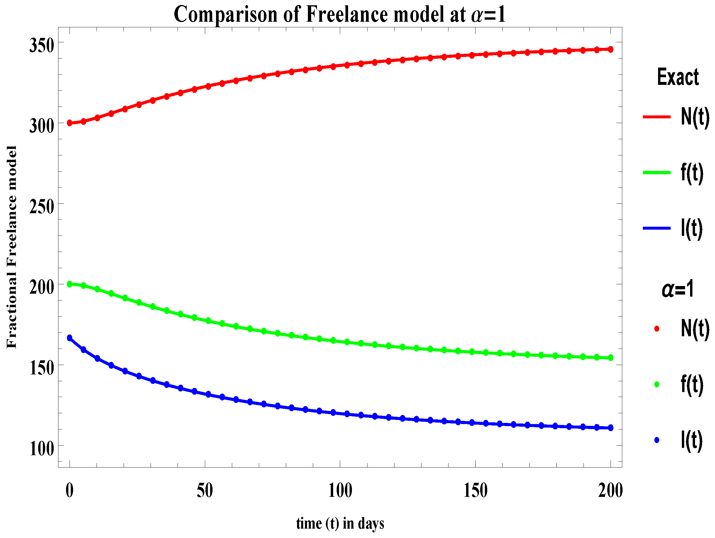
Results obtained graphically describes the impact of information on population about freelance. As in Figure 1, the comparison of fractional freelance model at $\alpha =1$ is given with the numerical solution of this model in [9] by keeping the parameters and initial values same in both papers. If we consider $a<b$, then it means that the negative information is prevailing among communities about freelancing and therefore we can observe the decline in $I\left(t\right)$ and $F\left(t\right)$. If people hear about bad experiences related to freelancing then they would not like to take risks with their stable income and therefore would not also suggest someone engage in freelancing. Hence, the population on $N\left(t\right)$ will increase.

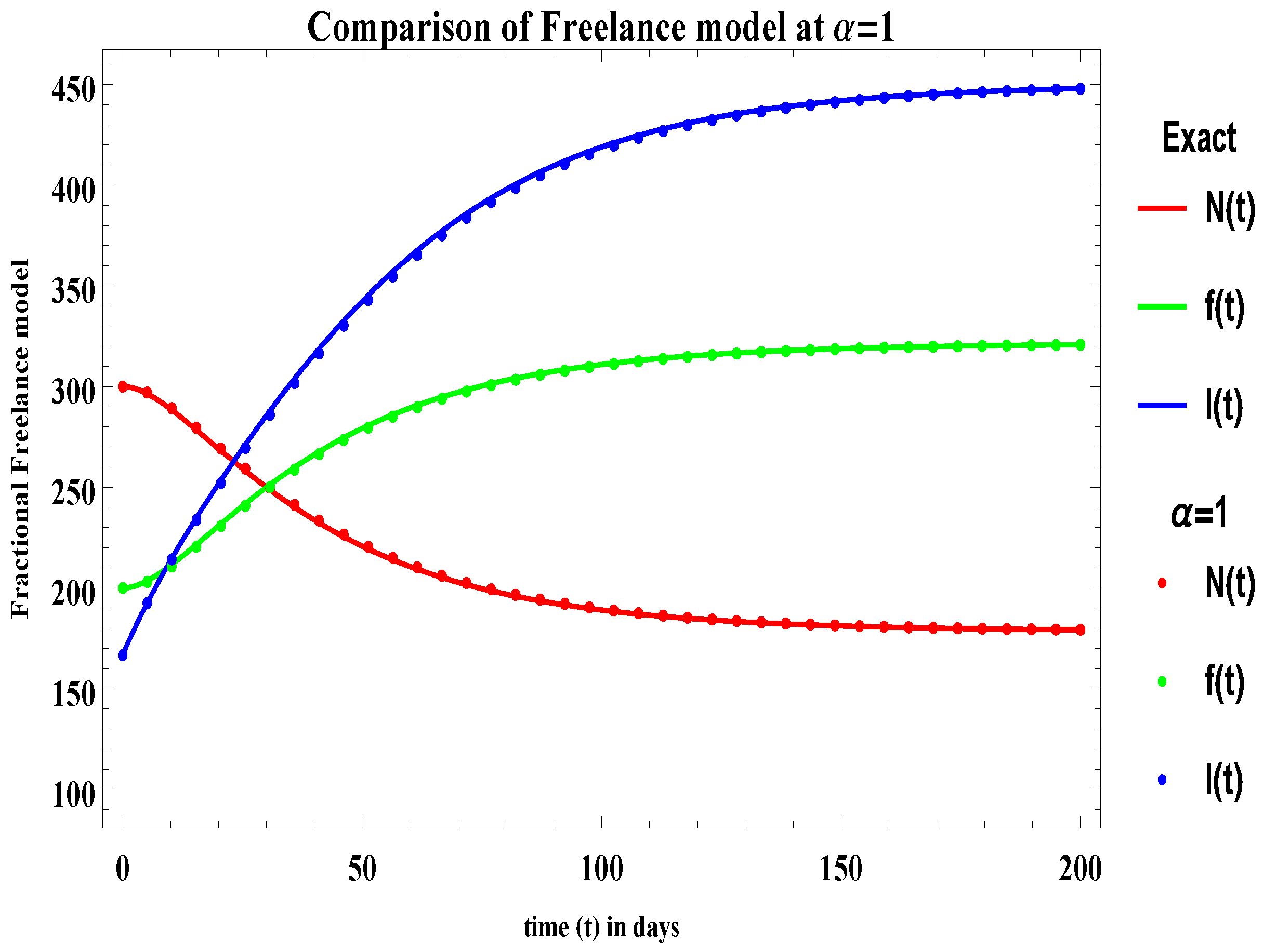
However, if we look at Figure 2, the situation where $a>b$ represents the increment in $F\left(t\right)$ and decrease in $N\left(t\right)$ by spreading the perks and positive impression of $I\left(t\right)$. Which is only possible if people around them observe freelancers doing well. Since freelancing is based on skills; therefore, to do well in this field one must have expertise to earn well thorough freelancing. It is actually a virtual business world and there are some techniques that one must learn to tackle the customer or how to enter the process and win the deal.

Figure 1 and Figure 2 and

Table 1. Comparison of freelance model variables in [9] with fractional freelance variable results at $\alpha =1$ for $a>b$.

t	$\mathit{N}\left(\mathit{t}\right)$	$\mathit{N}\left(\mathit{t}\right)$ at $\mathit{\alpha }=1$	$\mathit{F}\left(\mathit{t}\right)$	$\mathit{F}\left(\mathit{t}\right)$ at $\mathit{\alpha }=1$	$\mathit{I}\left(\mathit{t}\right)$	$\mathit{I}\left(\mathit{t}\right)$ at $\mathit{\alpha }=1$
0	300	300	200	200	166.667	166.667
50	220.736	221.575	279.264	278.425	342.343	340.503
100	189.051	189.096	310.949	310.904	418.945	418.808
150	181.172	181.135	318.828	318.865	441.948	442.06
200	179.22	179.199	320.78	320.801	447.969	448.036

clearly shows that this model is verified not only theoretically but graphically as well. So, this comparison clearly shows that we obtain the same results on $\alpha =1$ as on the model given in [9].

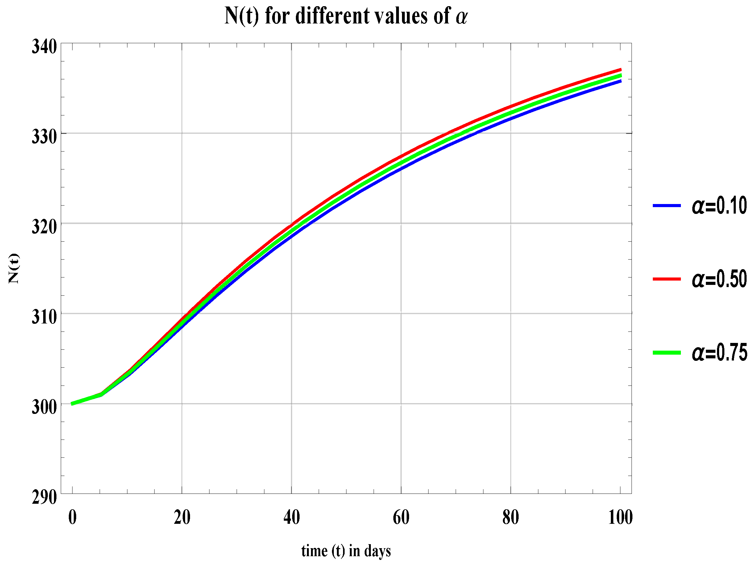
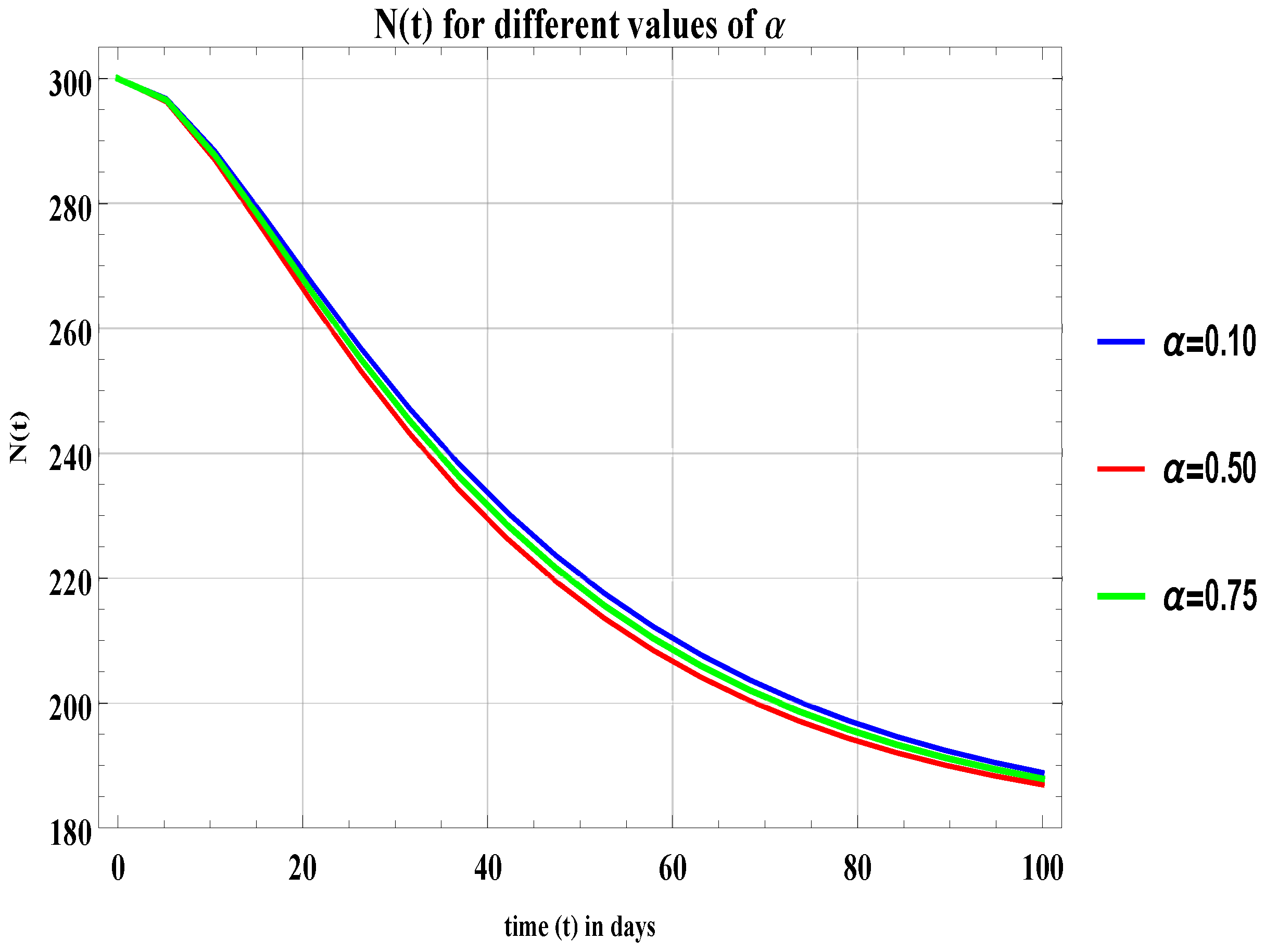
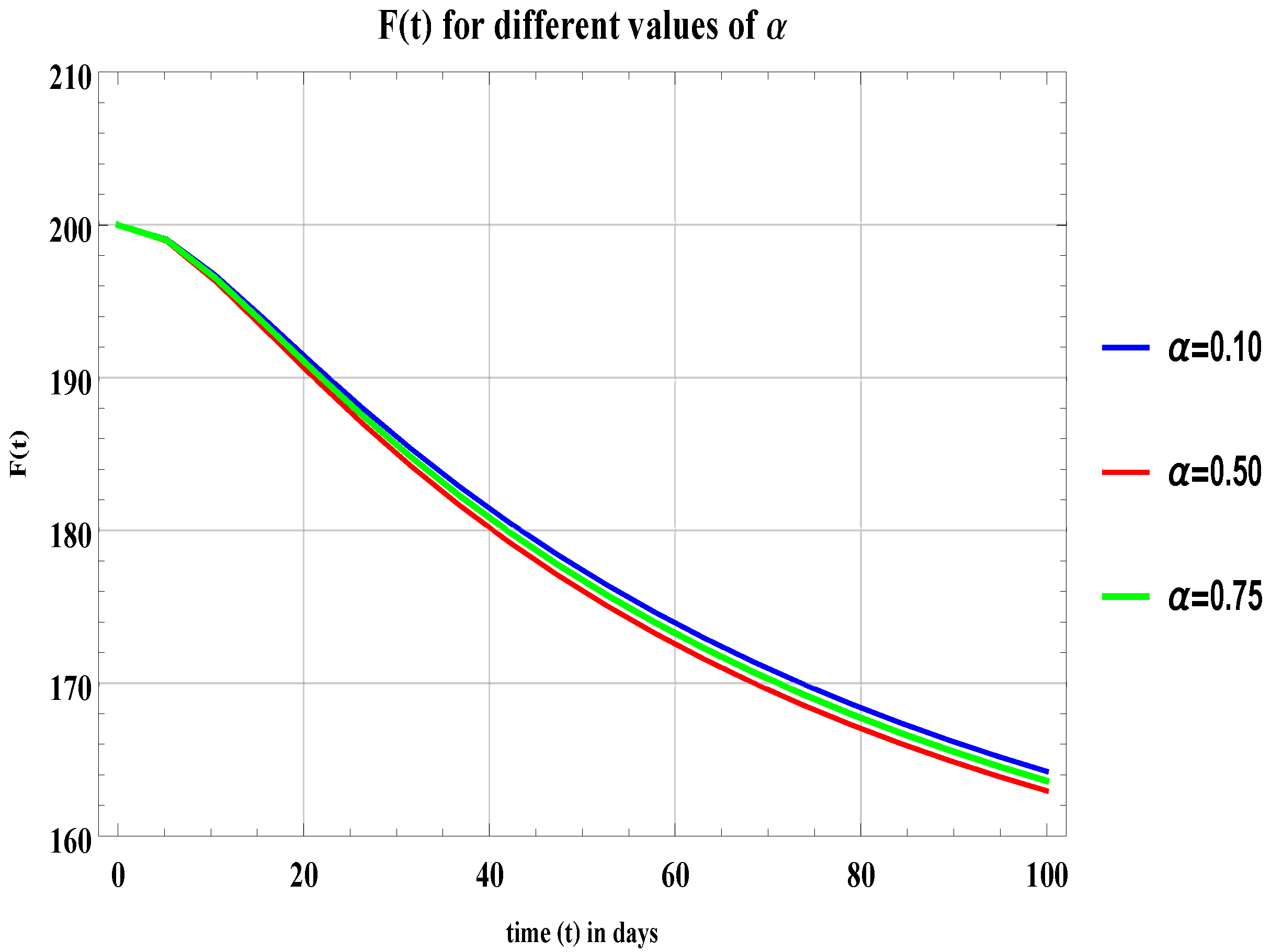
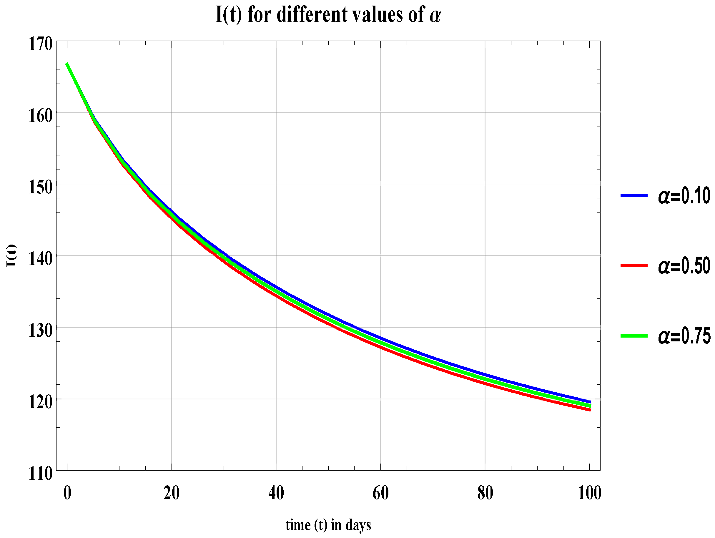
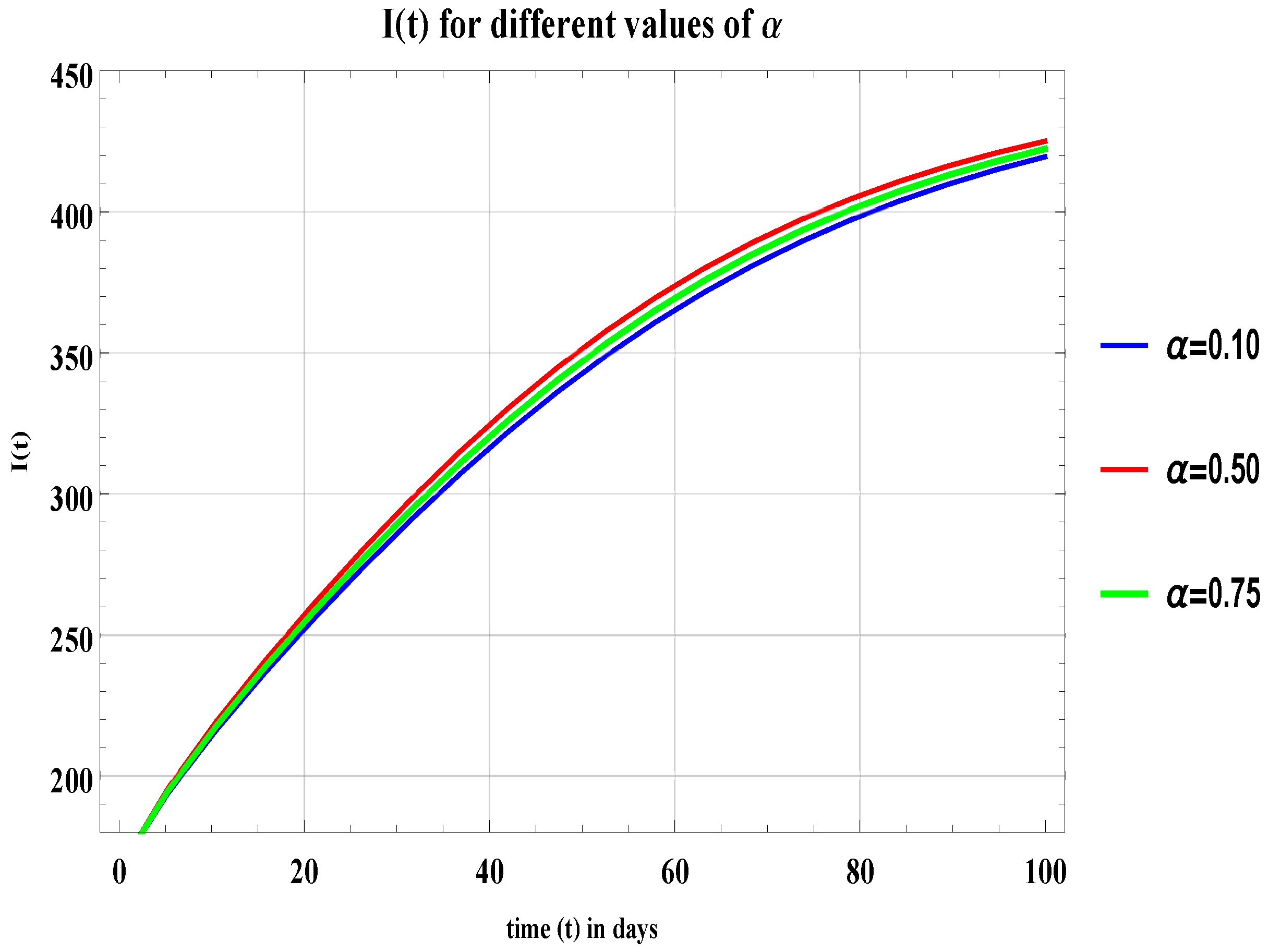
The graphical results in Figure 3 and Figure 4 and

Table 2. Results of $N\left(t\right)$ for different values of $\alpha$ for $a>b$.

t	$\mathit{\alpha }=0.2$	$\mathit{\alpha }=0.4$	$\mathit{\alpha }=0.6$	$\mathit{\alpha }=0.8$	$\mathit{\alpha }=1.0$
0	300	300	300	300	300
50	216.656	214.723	215.117	217.47	220.736
100	186.75	185.917	186.083	187.116	189.051
150	180.327	180.066	180.117	180.446	181.172
200	178.95	178.876	178.89	178.984	179.22

show the behavior of population of non-freelancers for different values of $\alpha$. As the graph shows, there is no significant change from $(0,1)$ for $\alpha =0.1, 0.5, 0.75$. The results of Figure 5, Figure 6, Figure 7 and Figure 8 are similar, i.e., if $a<b$ then $I\left(t\right)$ and $F\left(t\right)$ will decrease and if $a>b$ then $I\left(t\right)$ and $F\left(t\right)$ will increase.

Table 3. Results of $F\left(t\right)$ for different values of $\alpha$ for $a>b$.

t	$\mathit{\alpha }=0.2$	$\mathit{\alpha }=0.4$	$\mathit{\alpha }=0.6$	$\mathit{\alpha }=0.8$	$\mathit{\alpha }=1.0$
0	200	200	200	200	200
50	283.344	285.277	284.883	282.53	279.264
100	313.25	314.083	313.917	312.884	310.949
150	319.673	319.934	319.883	319.554	318.828
200	321.05	321.124	321.11	321.016	320.78

and

Table 4. Results of $I\left(t\right)$ for different values of $\alpha$ for $a>b$.

t	$\mathit{\alpha }=0.2$	$\mathit{\alpha }=0.4$	$\mathit{\alpha }=0.6$	$\mathit{\alpha }=0.8$	$\mathit{\alpha }=1.0$
0	166.667	166.667	166.667	166.667	166.667
50	351.021	355.262	354.392	349.253	342.343
100	425.449	427.849	427.37	424.403	418.945
150	444.537	445.344	445.186	444.17	441.948
200	448.813	449.043	448.999	448.705	447.969

also show the numerical values for the case $a>b$ for different values of $\alpha$.

For different values of $\alpha$ in all graphs and in Table 2, Table 3 and Table 4, an infinitesimal change can be observed, which means the populations of this field do not make random decisions and their behavior is not abrupt—they make informed decisions and then give time to things to work out. If it would not go in their favor or they want to switch the fields from freelancer to non-freelancer or from non-freelancer to freelancer then they do it permanently.

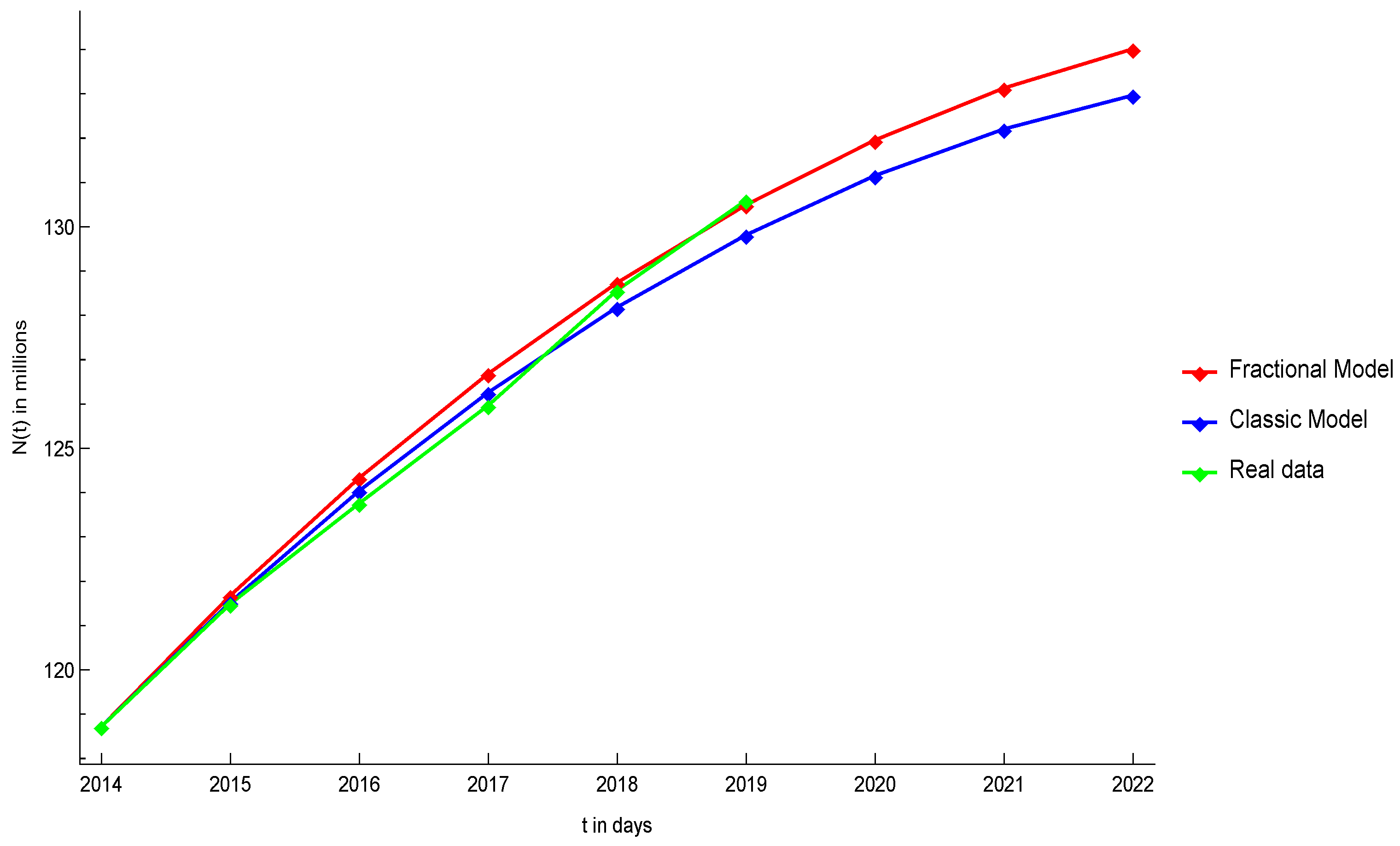
To verify the importance of this model in the real world as compared to the classical freelance model, we consider the real life data of US employees that are freelancers or non-freelancers.

Table 5. Number of freelancers and full time employees in the US.

Year	No of Freelancers (in Million) [30]	No of Employees (in Million) [29]
2014	53	118.72
2015	53.7	121.49
2016	55	123.76
2017	57.3	125.97
2018	56.7	128.57
2019	57	130.6

describes the data taken from [29,30] of freelancers and employees that are non-freelancers in the US; therefore, the parameter selection also varies according to the real data—parameters have value $\gamma =3.3$, $ϵ=0.0008$, $\delta =0.0008697$, $\mu =0.00089$, $a=0.06$, and $b=0.05$. In addition, for this solution, we consider, $N\left(0\right)=118.72,F\left(0\right)=53,I\left(0\right)=3$. All calculations are performed in the millions. Figure 9 shows the pattern of employees from 2014 to 2020 and shows that the fractional model is predicting it more accurately than the classic model of freelance. Figure 10 shows the pattern of freelancers from 2014 to 2020 and shows that the fractional model is predicting it more accurately than the classic model of freelance.

7. Conclusions

In this work, a new mathematical fractional model is formed by the fractional derivatives of Atangana–Baleanu–Caputo type. The uniqueness and existence of the solutions is proven by the Banach fixed point theory. For this, we use Schauder’s theorem to prove the existence of solution and fixed point theory to prove the uniqueness of this solution.

Numerically, the fractional freelance model is solved by using fractional Euler’s method based on ABC type fractional derivative. Two of its cases have been depicted graphically as well as in table form. If the positive information (i.e., $a>b$) is passed on or taught properly in institutions related to freelancing, then more people will choose freelancing as a career, which mathematically means $F\left(t\right), I\left(t\right)$ will increase with time and $N\left(t\right)$ will decrease with time. On the other hand, if negative information (i.e., $b>a$) is passed on, then not many people will join freelancing as a career and mathematically it means $F\left(t\right), I\left(t\right)$ will decrease with time and $N\left(t\right)$ will increase with time.

In addition, the comparison of this model at $\alpha =1$ with the classic freelance model and real data of US freelancers and non-freelancers is given in this work and clearly shows that the fractional model yields better predictions than the classic freelance model.

References

- Chang, F.X.; Chen, J.; Huang, W. The anomalous diffusion and fractional convection diffusion equation. Acta Phys. Sin. 2005, 54, 1113–1117. [Google Scholar] [CrossRef]
- Podlubny, I. Fractional Differential Equations; Academic Press: San Diego, CA, USA; Boston, MA, USA; New York, NY, USA, 1990. [Google Scholar]
- Povstenko, Y.Z. Fractional radial diffusion in a cylinder. J. Mol. Liq. 2008, 137, 46–50. [Google Scholar] [CrossRef]
- Wang, Z.T. Singular diffusion in fractal porous media. Appl. Math. Mech. 2000, 21, 1033–1038. [Google Scholar]
- Weeks, E.R.; Urbach, J.S.; Harry, L.S. Anomalous diffusion in asymmetric random walks with a quasi-geostrophic flow example. Phys. D Nonlinear Phenom. 1996, 97, 291–310. [Google Scholar] [CrossRef]
- Li, B.; Chen, Z.J.; Zhao, H.W. Application and development of rheology. Contemp. Chem. Ind. 2008, 37, 221–224. [Google Scholar]
- Khalid, M.; Khan, F.K. A fractional numerical solution and stability analysis of Facebook users mathematical model. In Proceedings of the 14th International Conference on Statistical Sciences, Karachi, Pakistan, 14–16 March 2016; Volume 29, pp. 323–334. [Google Scholar]
- Khalid, M.; Khan, F.S.; Iqbal, A. Perturbation iteration algorithm to solve fractional giving up smoking mathematical model. Int. J. Comput. Appl. 2016, 142, 1–6. Available online: https://www.ijcaonline.org/archives/volume142/number9/khalid-2016-ijca-909891.pdf (accessed on 2 August 2022). [CrossRef]
- Fareeha, S.K.; Khalid, M.; Ali, A.H.; Bazighifan, O.; Nofal, T.A.; Nonlaopon, K. Does freelancing have a future? Mathematical analysis and modeling. Math. Biosci. Eng. 2022, 19, 9357–9370. [Google Scholar]
- Upwork. Freelance Forward 2020; Edelman Intelligence/Upwork Inc.: Chicago, IL, USA, 2020. [Google Scholar]
- Payoneer. Freelancing in 2020: An Abundance of Opportunities; Payoneer: New York, NY, USA, 2020. [Google Scholar]
- National Freelancing Conference 2021 in Bhurban; Ministry of Information Technology and Telecommunication: Islamabad, Pakistan, 2021. Available online: https://Digitalpakistan.Pk. (accessed on 2 August 2022).
- National Freelancing Facilitation Policy 2021 Consultation Draft. (2021); Ministry of Information Technology and Telecommunication: Islamabad, Pakistan, 2021. Available online: https://moitt.gov.pk (accessed on 2 August 2022).
- Rawoof, H.A.; Ahmed, K.A.; Saeed, N. The role of online freelancing: Increasing women empowerment in Pakistan. Int. J. Disaster Recovery Bus. Continuity 2021, 12, 1179–1188. Available online: http://sersc.org/journals/index.php/IJDRBC/article/view/36681 (accessed on 2 August 2022).
- Masood, F.; Naseem, A.; Shamim, A.; Khan, A.; Qureshi, M.A. A systematic literature review and case study on influencing factor and consequences of freelancing in Pakistan. Int. J. Sci. Eng. Res. 2018, 9, 275–280. [Google Scholar]
- Saez-Marti, M. Siesta: A Theory of Freelancing; University of Zurich Department of Economics Working Paper; University of Zurich: Zurich, Switzerland, 2011. [Google Scholar] [CrossRef] [Green Version]
- Gupta, V.; Fernandez-Crehuet, J.M.; Gupta, C.; Hanne, T. Freelancing models for fostering innovation and problem solving in software startups: An empirical comparative study. Sustainability 2020, 12, 10106. [Google Scholar] [CrossRef]
- Gubachev, N.; Titov, V.; Korshunov, A. Remote occupation and freelance as modern trend of employment. In Proceedings of the 12th International Management Conference, Bucharest, Romania, 1–2 November 2018; pp. 725–732. Available online: http://conferinta.management.ase.ro/archives/2018/pdf/4_13.pdf (accessed on 2 August 2022).
- Kirchner, J.; Mittelhamm, E. Employee or freelance worker. In Key Aspects of German Employment and Labour Law; Springer: Berlin/Heidelberg, Germany, 2010; pp. 37–43. [Google Scholar] [CrossRef]
- Rasheed, M.; Ali, A.H.; Alabdali, O.; Shihab, S.; Rashid, A.; Rashid, T.; Abed Hamad, S.H. The Effectiveness of the Finite Differences Method on Physical and Medical Images Based on a Heat Diffusion Equation. J. Phys. Conf. Ser. 2021, 1999, 012080. [Google Scholar] [CrossRef]
- Qaraad, B.; Bazighifan, O.; Nofal, T.A.; Ali, A.H. Neutral Differential Equations with Distribution Deviating Arguments: Oscillation Conditions. J. Ocean. Eng. Sci. 2022; in press. [Google Scholar]
- Sultana, M.; Arshad, U.; Ali, A.H.; Bazighifan, O.; Al-Moneef, A.A.; Nonlaopon, K. New Efficient Computations with Symmetrical and Dynamic Analysis for Solving Higher-Order Fractional Partial Differential Equations. Symmetry 2022, 14, 1653. [Google Scholar] [CrossRef]
- Moaaz, O.; Chalishajar, D.; Bazighifan, O. Asymptotic Behavior of Solutions of the Third Order Nonlinear Mixed Type Neutral Differential Equations. Mathematics 2020, 8, 485. [Google Scholar] [CrossRef]
- Moaaz, O.; Bazighifan, O. Oscillation Criteria for Second-Order Quasi-Linear Neutral Functional Differential Equation. Discrete Contin. Dyn. Syst. Ser. S 2020, 13, 2465–2473. [Google Scholar] [CrossRef] [Green Version]
- Tunc, C.; Bazighifan, O. Some new oscillation criteria for fourth-order neutral differential equations with distributed delay. Electr. J. Math. Anal. Appl 2019, 7, 235–241. [Google Scholar]
- Caputo, M.; Fabrizio, M. A New Definition of Fractional Derivative without Singular Kernel. Progr. Fract. Differ. Appl. 2015, 1, 73–85. [Google Scholar]
- Atangana, A.; Baleanu, D. New fractional derivatives with non-local and non-singular kernel: Theory and application to heat transfer model. Therm. Sci. 2016, 20, 763–769. [Google Scholar] [CrossRef] [Green Version]
- Khan, F.S.; Khalid, M.; Bazighifan, O.; El-Mesady, A. Euler’s Numerical Method on Fractional DSEK Model under ABC Derivative. Complexity 2022, 2022, 4475491. [Google Scholar] [CrossRef]
- Statista Research Department. Number of Full-Time Employees in the United States from 1990–2021. Statista 2022. Available online: https://www.statista.com/statistics/192356 (accessed on 2 August 2022).
- Statista Research Department. Number of Freelance Workers in the United States from 2014 to 2020. Statista 2022. Available online: https://www.statista.com/statistics/685468/amount-of-people-freelancing-us/ (accessed on 2 August 2022).
Figure 1.
Comparison of fractional freelance model at and with its ODE numerical solution [9] for and .
Figure 2.
Comparison of fractional freelance numerical solution at and with its ODE numerical solution [9] for and .
Figure 3.
Graph of for , , and .
Figure 4.
Figure 5.
Figure 6.
Figure 7.
Figure 8.
Figure 9.
Comparison of fractional freelance at model, classical freelance model, and actual data collected in Table 5 for the number of workers in US that are non-freelancers.
Figure 10.
Comparison of fractional freelance at , classical freelance model, and actual data collected in Table 5 for the number of freelancers in the US. Further, predicting the future trend for freelancers in the US.