
LARO: Opposition-Based Learning Boosted Artificial Rabbits-Inspired Optimization Algorithm with Lévy Flight


1
Electronic Information and Electrical Engineering College, Shangluo University, Shangluo 726000, China
2
College of Mathematics and Computer Application, Shangluo University, Shangluo 726000, China
3
Department of Applied Mathematics, Xi’an University of Technology, Xi’an 710054, China
*
Author to whom correspondence should be addressed.
Symmetry 2022, 14(11), 2282; https://doi.org/10.3390/sym14112282
Submission received: 8 October 2022
/
Revised: 24 October 2022
/
Accepted: 26 October 2022
/
Published: 31 October 2022
Abstract
:The artificial rabbits optimization (ARO) algorithm is a recently developed metaheuristic (MH) method motivated by the survival strategies of rabbits with bilateral symmetry in nature. Although the ARO algorithm shows competitive performance compared with popular MH algorithms, it still has poor convergence accuracy and the problem of getting stuck in local solutions. In order to eliminate the effects of these deficiencies, this paper develops an enhanced variant of ARO, called Lévy flight, and the selective opposition version of the artificial rabbit algorithm (LARO) by combining the Lévy flight and selective opposition strategies. First, a Lévy flight strategy is introduced in the random hiding phase to improve the diversity and dynamics of the population. The diverse populations deepen the global exploration process and thus improve the convergence accuracy of the algorithm. Then, ARO is improved by introducing the selective opposition strategy to enhance the tracking efficiency and prevent ARO from getting stuck in current local solutions. LARO is compared with various algorithms using 23 classical functions, IEEE CEC2017, and IEEE CEC2019 functions. When faced with three different test sets, LARO was able to perform best in 15 (65%), 11 (39%), and 6 (38%) of these functions, respectively. The practicality of LARO is also emphasized by addressing six mechanical optimization problems. The experimental results demonstrate that LARO is a competitive MH algorithm that deals with complicated optimization problems through different performance metrics.
1. Introduction
Most practical applications of problem processing often go to the appropriate solution of an optimization problem by their very nature [1]. Therefore, the optimization problem has been a problem that has received much attention from the beginning, and the exploration of various efficient methods for complicated optimization problems (COPs) has captured the attention of scholars in many fields. Among them, the traditional mathematical optimization method as an optimization strategy requires that the associated objective function needs meet convexity and separability. This property requirement guarantees that it approximates the optimal solution theoretically. However, traditional mathematical strategies are complicated in dealing with highly complex and demanding optimization problems [2]. Newton’s method and the branch-and-bound method are typical deterministic algorithms. Although such algorithms are superior to metaheuristic nature-inspired algorithms in solving some single-parameter tests in terms of functional tests, deterministic algorithms tend to fall into local optimal solutions when faced with more demanding objective functions and constraint functions. Deterministic methods may not be effective when facing multimodal, discrete, non-differentiable, or non-convex problems, or with a comprehensive search space. In addition, deterministic algorithms sometimes require a derivative. Therefore, deterministic algorithms often do not work in solving engineering problems [3].
MH techniques have recently attracted more scholarly attention because of their unique idea of providing a suitable candidate to handle various complex and realistic optimization problems. In general, MH methods have some available advantages over traditional mathematical optimization methods: MH algorithms are an efficient search, low-complexity global optimization method, and different solutions can be searched for in each iteration, making these other solutions highly competitive in obtaining optimal solutions [4].
Depending on the object of construction, experts tend to classify MH algorithms into four parts: evolution-based algorithms, group-intelligence-based algorithms, physical- or chemical-based algorithms, and human-behavior-based algorithms (HBAs) [5]. Evolution-based algorithms imitate the natural evolutionary laws of the biological world; examples of this category include genetic algorithms [6], evolutionary strategies [7], differential evolution [8] which is a variation, crossover, and selection-based garlic algorithm, and evolutionary planning (EP) [9].
Group-intelligence-based (GIB) algorithms are often motivated by the cooperative conduct of various plants and animals in natural environments that live in groups and work together to find food/prey. This GIB category includes aphid–ant mutualism (AAM) [10], bottlenose dolphin optimizer (BDO) [11], beluga whale optimization (BWO) [12], capuchin search algorithm (CapSA) [13], sand cat swarm optimization (SCSO) [14], manta ray foraging optimization algorithm (MRFO) [15], black widow optimization algorithm (BWOA) [16], and chimp optimization algorithm (CHOA) [17].
A physical- or chemical-based algorithm simulates the physical laws and chemical phenomena of biological nature, usually following a generic set of rules to discriminate the influence of interactions between candidate solutions. The type includes the gravitational search algorithm [18], a popular physical- or chemical-based algorithm motivated by Newton’s law of gravity. According to some gravitational force, subjects are attracted to each other according to the law of gravitation. Examples include atom search optimization [19], ion motion algorithm [20], equilibrium optimizer [21], and water cycle algorithm (WCA) [22].
In the last case of the four types, HBAs are exploited by taking advantage of various characteristics associated with humans. The main types of this category include human mental search [23], poor and rich optimization algorithm [24], and teaching learning-based optimization [25].
Dealing with COPs usually consists of two steps: exploration and exploitation. Exploration and exploitation are two opposite strategies. The algorithm searches for a better solution in the global discovery domain in the exploration step. In the development step, the algorithm tends to locate the best solution found so far by exploring the vicinity of the candidate solutions. The trade-off between exploration and exploitation is considered one of the most common problems in current metaheuristic algorithms [26]. This general problem forces the optimization search process to utilize one of the search mechanisms at the expense of the other strategy. In this context, many scholars have proposed algorithms to balance such mechanisms. For example, Zamani proposed a quantum-based avian navigation optimizer algorithm inspired by the navigation behavior of migratory birds [27]. In addition, Nadimi-Shahraki introduced the proposed multi-trial vector approach and archiving mechanism to the differential evolution algorithm, thus proposing a diversity-maintained differential evolution algorithm [28]. ARO was suggested as a newly developed metaheuristic technique with steps inspired by the laws of rabbit survival in the natural world [29].
Regarding the no-free-lunch theory [30], no nature-inspired method can optimally handle every realistic COP [31]. The above facts imply that optimization methods are applied to solve specific COPs but may not be valid for solving other COPs, and experimental results tend to reveal that artificial rabbits optimization has poor convergence accuracy and tends to get stuck in local solutions when handling complicated or high-latitude issues. Therefore, based on the importance of the above two reasons, this paper suggests a hybrid artificial rabbit optimization with Lévy flight and selective opposition strategy, called enhanced ARO algorithm (LARO). LARO is a variant of the ARO algorithm. First, to enhance the worldwide finding capability of ARO, the Lévy flight strategy is fully utilized [32]. The Lévy flight strategy helps LARO to design local solution avoidance and international exploration. Secondly, local exploitation of LARO is achieved by using a selective opposition strategy with improved convergence accuracy [33]. The innovative points and the major contributions of this paper are given below:
- (i)
- The Lévy flight strategy is introduced in the random hiding phase to improve the diversity and dynamics of the population, which further improves the convergence accuracy of ARO.
- (ii)
- The introduced selection opposition strategy extends the basic opposition strategy and adaptively re-updates the algorithm to improve the ability to jump out of the local optimum.
- (iii)
- Numerical experiments are tested on 23 standard test functions, the CEC2017 test set, and the CEC2019 test set.
- (iv)
- LARO is implemented and tested on six engineering design cases.
The remainder of this study is organized as given below. Section 2 describes the ARO mathematical model. The Lévy flight strategy, selective opposition strategy, and LARO algorithm are introduced in Section 3. Section 4 presents the numerical results and discussion of the proposed algorithm, mainly applied to 23 benchmark functions and the CEC2019 test set. An application of LARO to six real engineering problems is described in Section 5. Section 6 concludes this research work and discusses future prospects.
2. Artificial Rabbits Optimization (ARO)
The ARO algorithm is proposed mainly by referring to two laws of rabbit survival in the natural world: detour foraging and random hiding [29]. Among them, detour foraging is an exploration strategy to prevent detection by natural predators by having rabbits eat the grass near the nest. Random hiding is a strategy in which rabbits move to other burrows, mainly to hide further. The beginning of any search algorithm relies on the initialization process. Considering that the size of the design variable has dimension d, the size of the artificial rabbit colony is N, and the upper and lower limits are ub and lb. Then the initialization is done as follows.
where denotes the position of the jth dimension of the ith rabbit and r is a random number that we are given along with it.
The metaheuristic algorithm mainly considers the two processes of exploration and exploitation, while detour foraging mainly considers the exploration phase. Detour foraging is the tendency of each rabbit to stir around the food source and explore another rabbit location randomly chosen in the group to obtain enough food. The updated formula for detour foraging is given below.
where denotes the new position of the artificial rabbit, i,j = 1, …, N. denotes the position of the ith artificial rabbit, and represents artificial rabbits at other random positions. Tmax is the maximum number of iterations. [·] symbolizes the ceiling function, which represents rounding to the nearest integer, and randp represents a stochastic arrangement from 1 to d random permutation of integers. r1, r2, and r3 are stochastic numbers from 0 to 1. L represents the running length, which is movement speed when detour foraging. n1 obeys the standard normal distribution. The perturbation is mainly reflected by the normal distribution random number of n1. The perturbation of the last term of Equation (2) can help ARO avoid local extremum and perform a global search.
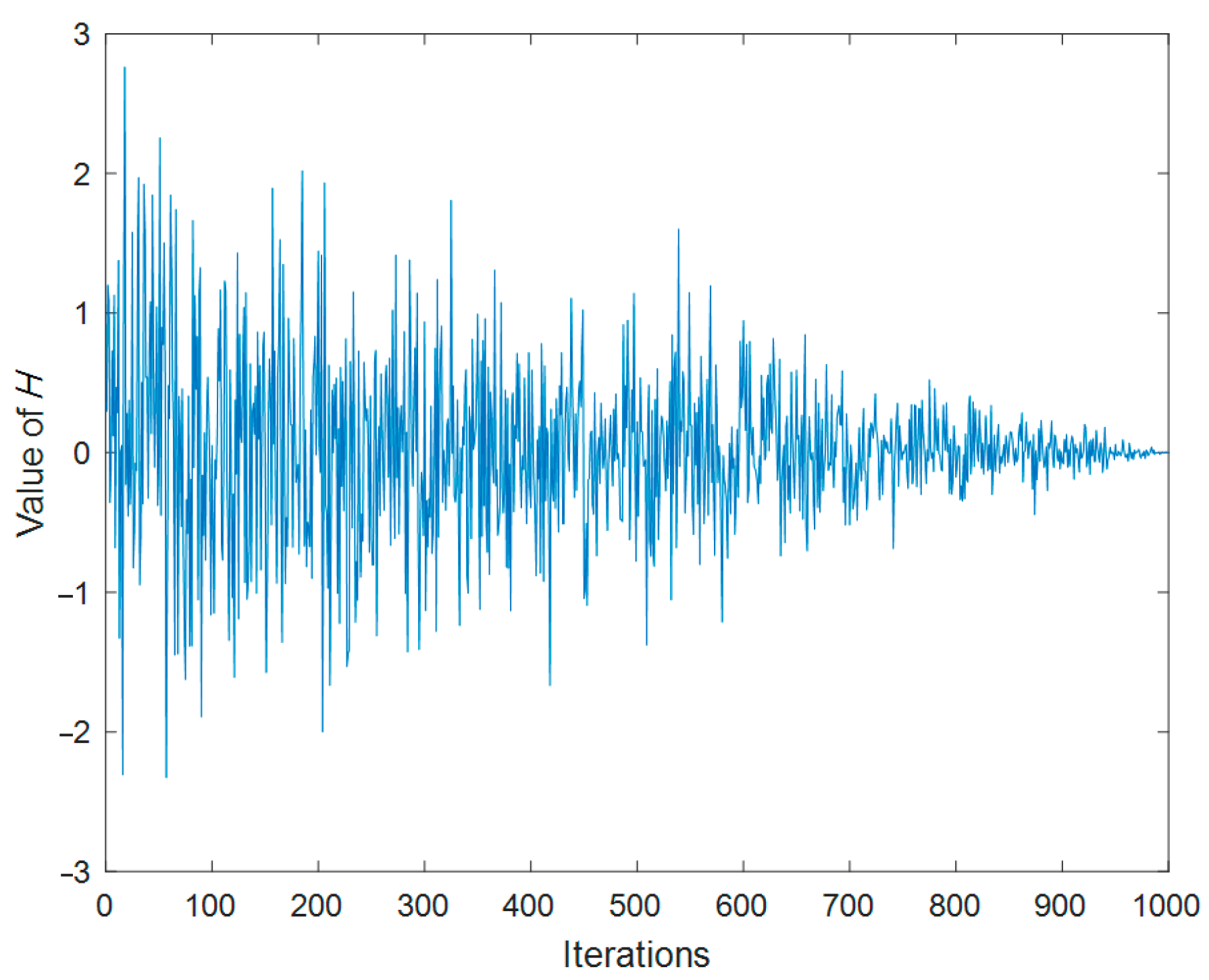
Random hiding is mainly modeled after the exploration stage of the algorithm, where rabbits usually dig several burrows around their nests and randomly choose one to hide in to reduce the probability of being predated. We first define the process by which rabbits randomly generate burrows. The ith rabbit produces the jth burrow by:
where i = 1, …, N and j = 1, …, d, and n2 follows the standard normal distribution. H denotes the hidden parameter that decreases linearly from 1 to 1/Tmax with stochastic perturbations. Figure 1 shows the change in the value of an over the course of 1000 iterations. In the figure, the H value trend generally decreases, thus maintaining a balanced transition from exploration to exploitation throughout the iterations.
The update formula for the random hiding method is shown below.
where is the new position of the artificial rabbit, represents a randomly selected burrow among the d burrows generated by the rabbit for hiding, and r4 and r5 represent the random number given by us in the interval 0 to 1. R is given by Equations (3)–(6).
After the two update strategies are implemented, we renew the position of the ith artificial rabbit by Equation (15).
This equation represents an adaptive update. The rabbit automatically chooses whether to stay in its current position or move to a new one based on the adaptation value.
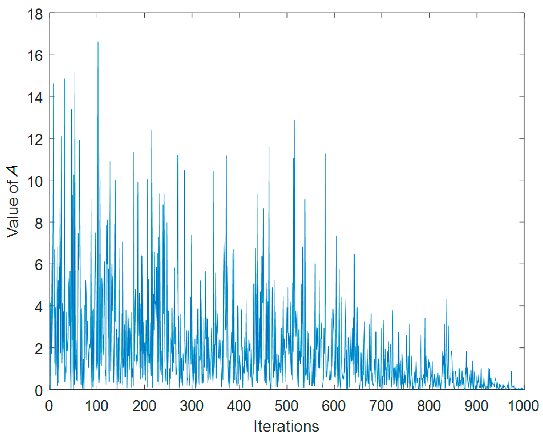
For an optimization algorithm, populations prefer to perform the exploration phase in the early stages and an exploitation phase in the middle and late stages. ARO relies on the energy of the rabbits to design a finding scheme: the rabbits’ energy decreases over time, thus simulating the exploration to exploitation transition. The definition of the energy factor in the artificial rabbits algorithm we give is:
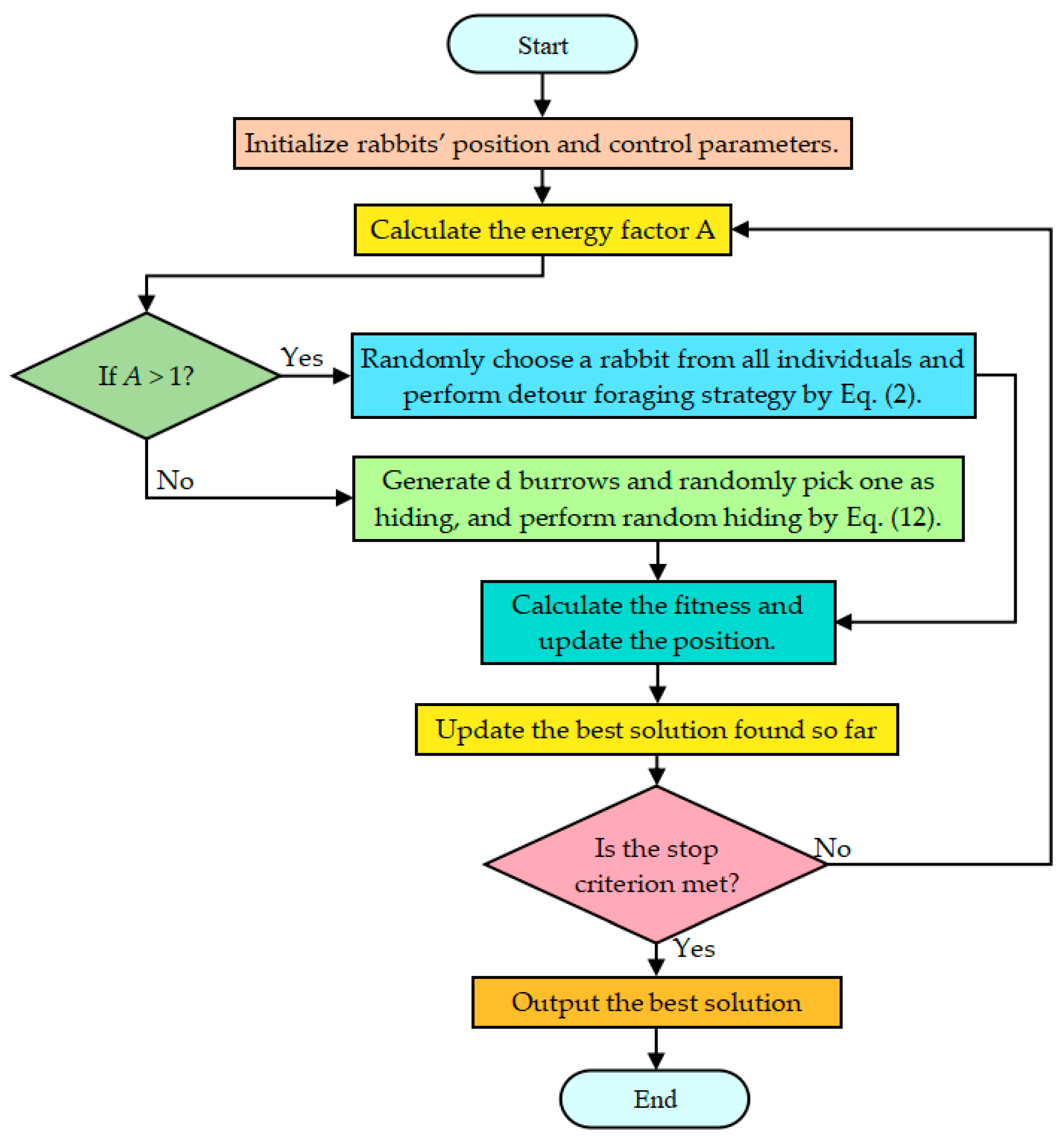
where r is a given random number and r is the random number in (0, 1). Figure 2 shows the change in the value of an over the course of 1000 iterations. Analysis of the information in the figure shows that the trend in the value of A’s is that the overall situation is decreasing, thus maintaining a balanced transition from exploration to exploitation throughout the iterations. Algorithm 1 gives the pseudo-code of the fundamental artificial rabbits optimization. Figure 3 provides the flow chart of ARO.
| Algorithm 1: The framework of artificial rabbits optimization |
| 1: The parameters of artificial rabbits optimization including the size of artificial rabbits N, and TMax. |
| 2: Random initializing a set of rabbits zi and calculate fi. |
| 3: Find the best rabbits. |
| 4: While t ≤ TMax do |
| 5: For i = 1 to N do |
| 6: Calculate the energy factor A by Equation (16). |
| 7: If A > 1 then |
| 8: Random choose a rabbits from all individuals. |
| 9: Compute the R using Equations (3)–(6). |
| 10: Perform detour foraging strategy by Equation (2). |
| 11: Calculate the fitness value of the rabbit’s position fi. |
| 12: Updated the position of rabbit by Equation (15). |
| 13: Else |
| 14: Generate d burrows and select one randomly according to Equation (14). |
| 15: Perform random hiding strategy by Equation (12). |
| 16: Calculate the fitness value of the rabbit’s position fi. |
| 17: Updated the position of rabbit by Equation (15). |
| 18: End if |
| 19: End for |
| 20: Search for the best artificial rabbit. |
| 21: t = t + 1. |
| 22: End while |
| 23: Output the most suitable artificial rabbit. |
3. Hybrid Artificial Rabbits Optimization
Hybrid optimization algorithms are widely used in practical engineering due to targeted improvements to the original algorithm that enhance the different performances of the algorithm. For example, Liu proposed a new hybrid algorithm that combines particle swarm optimization and single layer neural network to achieve the complementary advantages of both and successfully implemented in wavefront shaping [34]. Islam effectively solves the clustered vehicle routing problem by combining particle swarm optimization (PSO) and variable neighborhood search (VNS), fusing the diversity of solutions in PSO and bringing solutions to local optima in VNS [35]. Devarapalli proposed a hybrid modified grey wolf optimization–sine cosine algorithm that effectively solves the power system stabilizer parameter tuning in a multimachine power system [36]. To mitigate the poor accuracy and ease of falling into local solutions of the original ARO algorithm, we propose a hybrid, improved LARO algorithm by introducing a Lévy flight strategy and selective opposition in the ARO algorithm and applying the proposed algorithm to engineering optimization problems. Among them, Lévy flight is employed to boost the algorithm’s accuracy. The selective opposition strategy helps the algorithm jump out of local solutions.
3.1. Lévy Flight Method
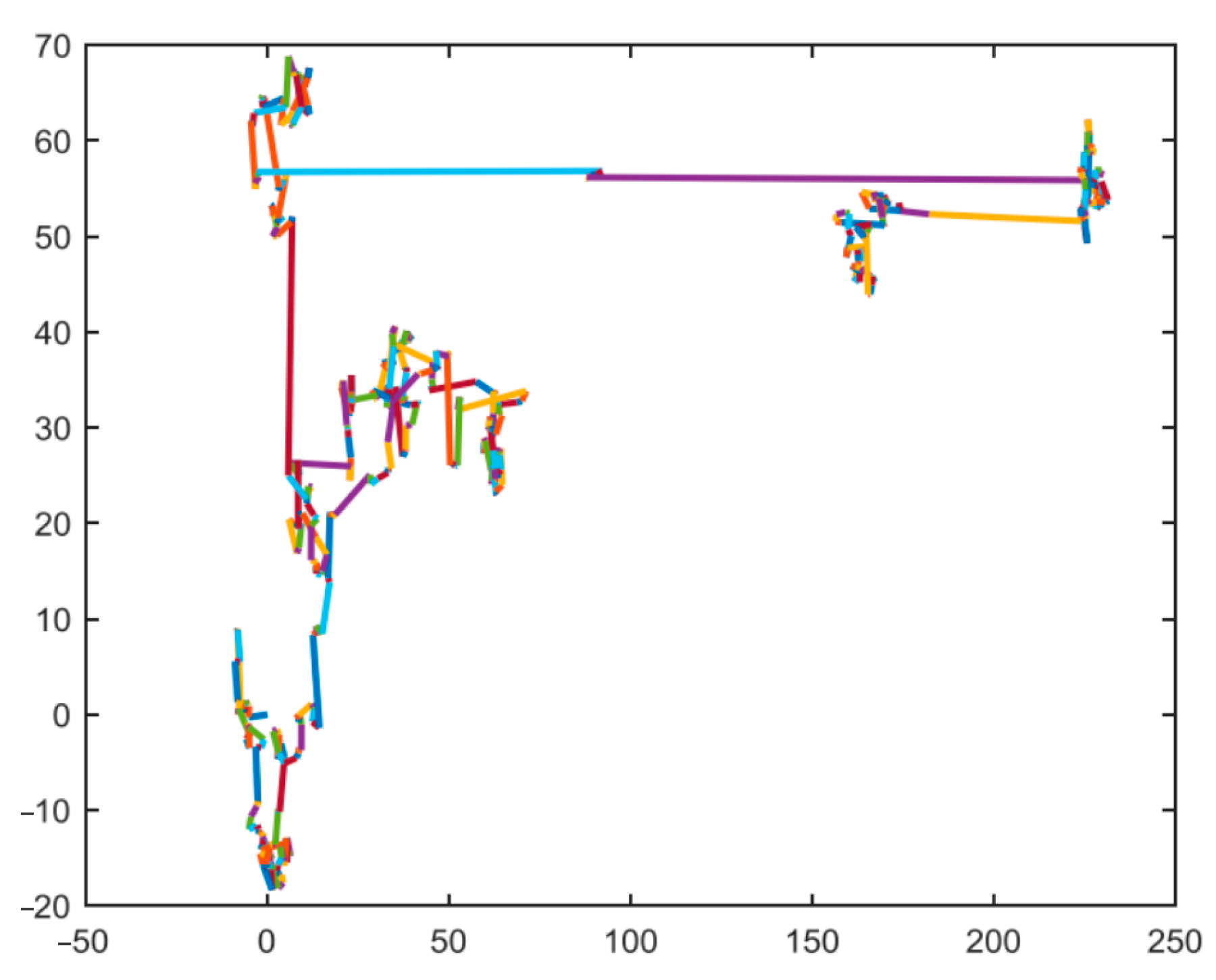
The Lévy flight method is often introduced in improved algorithms and proposed algorithms, mainly to provide dynamism to the algorithm updates, where the Lévy flight operator is mentioned primarily for generating a regular random number, which is characterized as a small number in most cases and a large random number in few cases. This arbitrary number generation law can help various update strategies to provide dynamics and jump out of local solutions. Lévy distribution is defined by the following equation. Figure 4 provides Levy’s flight path in two-dimensional space [32].
where t is the step length, which can be calculated by Equation (18). The formulas for solving the step size of the Lévy flight are given in Equations (18)–(21).
where σu and σv are defined as given in Equations (20) and (21). Both u and v obey Gaussian distributions with mean 0 and variance σu2 and σv2, as shown in Equation (19). Γ denotes a standard Gamma function, while β denotes a correlation parameter, which is usually set to 1.5.
In the random hiding phase, we replace the r4 random numbers with the random numbers generated by the Lévy flight strategy. Since the random hiding stage is an exploitation stage, we introduce Lévy flight in this strategy to avoid ARO from falling into local candidate solutions in the exploitation phase. Additionally, it helps the algorithm improve the convergence accuracy and the flexibility of the random hiding stage. The following equation provides the random hidden phase based on the Lévy flight, where α is a parameter fixed to 0.1.
3.2. Selective Opposition (SO) Strategy
SO is a modified idea of opposition-based learning (OBL) [33]. The idea of SO is to modify the size of the rabbits far from the optimal solution by using new opposition-based learning to bring it closer to the rabbit in the optimal position. In addition, the selective opposition strategy tends to be affected by a linearly decreasing threshold. When the rabbits deploy SO, selective opposition assists the rabbits in achieving a better situation in the development phase by changing the proximity dimension of different rabbits [37]. The updates are as follows.
First, we define a threshold value. The threshold value will be decreased until the limit case is reached. As shown in the following equation, SO checks the distance of each candidate rabbit location from the current rabbit dimension to the best rabbit location for all candidate rabbit locations.
where ddj is the difference distance of all dimensions of each rabbit. When ddj is greater than the Threshold (TS) value we define, the far and near rabbit positions are calculated. Then, all difference distances for all rabbit positions are listed.
The src is proposed mainly to measure the correlation between the current rabbit and the optimal rabbit position. Assuming that src < 0 and the far dimension (df) is larger than the close dimensions (dc), the rabbit’s position will be updated by Equation (25).
Algorithm 2 gives the pseudo-code for selective opposition (SO).
| Algorithm 2: Selective Opposition (SO) |
| 1: The parameters of selective opposition including: initial generation (t), rabbit size (N), the maximum generation (TMax), dimension (d), dc = [], and df = []. |
| 2: TS = 2 − [t·(2/TMax)]. |
| 3: For i = 1 to N do |
| 4: If Zi ≠ Zibest then |
| 5: For j = 1 to d do |
| 6: ddj = |zibest,j-zi,j|{ddj = the discrepancy distance of the jth dimension} |
| 7: If ddj < TS then |
| 8: Determine the far dimensions (df). |
| 9: Calculate far distance dimensions (df). |
| 10: Else |
| 11: Determine the close dimensions (dc). |
| 12: Calculate close distance dimensions (dc). |
| 13: End if |
| 14: End for |
| 15: Summing over all ddj. |
| 16: . |
| 17: If src ≤ 0 and size(df) > size(dc) then |
| 18: Perform Z′df = LBdf + UBdf − Zdf. |
| 19: End if |
| 20: End if |
| 21: End for |
3.3. Detailed Implementation of LARO
Two modifications, namely Lévy flight and selective opposition, are included in ARO. These modifications suitably help the ARO algorithm to increase the convergence and population variety while obtaining more qualitative candidate solutions. The detailed procedures of LARO are shown below.
Step1: Suitable parameters for LARO are supplied: the size of artificial rabbit N, the dimensionality of the variables d, the upper and lower bounds ub and lb of the problem variables, and all iterations TMax;
Step2: Randomly select a series of rabbit locations and calculate their fitness values. Find the rabbit with the best position;
Step3: Calculate the value of the energy factor A by Equation (16). If A > 1, select an arbitrary rabbit from all groups of rabbits;
Step4: Calculate the value of R by using Equations (3)–(6). Perform detour foraging strategy by means of Equation (2). Then calculate the adaptation value of the updated rabbit position and update the rabbit position by means of Equation (15);
Step5: If A ≤ 1, randomly generate burrows and randomly select one according to Equation (14). The new position of the rabbit is updated by a random hiding strategy based on the improved Lévy flight strategy of Equation (22). The corresponding fitness is calculated and then the rabbit’s position is updated by Equation (15);
Step6: The distance of each candidate rabbit position from the current rabbit dimension to the best rabbit position is calculated by Equation (23);
Step7: If ddj > Threshold, determine the near size df and count the number of df. If ddj ≤ Threshold, determine the far dimension dc and count the number of dc. Then calculate src from the calculated ddj by Equation (24);
Step8: If src <= 0 and df > dc, execute Equation (25) and re-update the rabbit’s position;
Step9: If the iterations exceed the maximum case, the optimal result is exported.
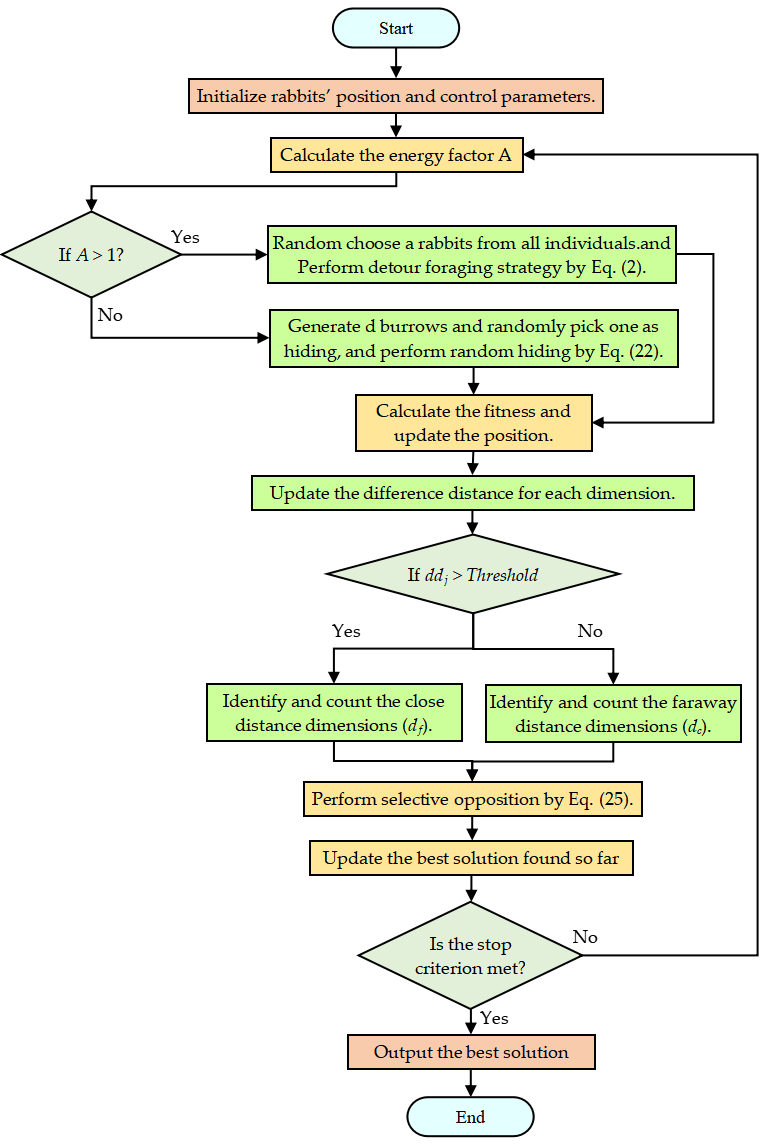
To better introduce the proposed LARO algorithm in this study, the pseudo-code of LARO is offered in Algorithm 3. Among them, line 15 is the Lévy flight strategy improved with the random hiding strategy. Lines 20–40 are the selective opposition strategy. Figure 5 illustrates the flowchart of the LARO algorithm.
| Algorithm 3: The algorithm composition of LARO |
| 1: The parameters of artificial rabbits optimization: the size of artificial rabbits N, TMax, the sensitive parameter α, β, dc = [], and df = []. |
| 2: Random initializing a set of rabbits zi and calculate fi. |
| 3: Find the best rabbits. |
| 4: While t ≤ TMax do |
| 5: For i =1 to N do |
| 6: Compute the energy factor A using Equation (16). |
| 7: If A > 1 then |
| 8: Random choose a rabbits from all individuals. |
| 9: Compute the R using Equations (3)–(6). |
| 10: Perform detour foraging strategy by Equation (2). |
| 11: Calculate the fitness value of the rabbit’s position fi. |
| 12: Updated the position of rabbit by Equation (15). |
| 13: Else |
| 14: Generate d burrows and select one randomly according to Equation (14). |
| 15: Perform random hiding strategy by Equation (22). |
| 16: Calculate the fitness value of the rabbit’s position fi. |
| 17: Updated the position of rabbit by Equation (15). |
| 18: End if |
| 19: End for |
| 20: TS = 2 − [t·(2/TMax)]. |
| 21: For i = 1 to N do |
| 22: If Zi ≠ Zibest then |
| 23: For j = 1 to d do |
| 24: ddj = |zibest,j-zi,j|{ddj = the discrepancy distance of the jth dimension} |
| 25: If ddj < TS then |
| 26: Determine the far dimensions (df). |
| 27: Calculate far distance dimensions (df). |
| 28: Else |
| 29: Determine the close dimensions (dc). |
| 30: Calculate close distance dimensions (dc). |
| 31: End if |
| 32: End for |
| 33: Summing over all ddj. |
| 34: . |
| 35: If src ≤ 0 and size(df) > size(dc) then |
| 36: Perform Z′df = LBdf + UBdf − Zdf. |
| 37: End if |
| 38: End if |
| 39: End for |
| 40: Updated the position of rabbit by Equation (15). |
| 41: Search for the best rabbits bestj. |
| 42: t = t + 1. |
| 43: End while |
| 44: Output the most suitable artificial rabbit. |
3.4. In-Depth Discussion of LARO Complexity
The estimation of LARO complexity is mainly done by adding the selective opposition part to the ARO base algorithm. At the same time, the Lévy strategy only improves how ARO is updated without increasing the complexity. Calculating the complexity is an effective method when assessing the complexity of solving real problems. The complexity is associated with the size of artificial rabbits N, d, and TMax. The total complexity of the artificial rabbits algorithm is as follows [29].
The selective opposition strategy focuses on the consideration of all dimensions of all rabbit locations. Therefore, the complication of the LARO algorithm is:
4. Numerical Experiments
To numerically experimentally validate the capabilities of the LARO algorithm, two basic suites were selected: 23 benchmark test functions [26] and ten benchmark functions from the standard CEC2019 test suite [26]. We selected some optimized metaheuristic algorithms to compare with our proposed LARO, including arithmetic optimization algorithm (AOA) [38], grey wolf optimization (GWO) [39], coot optimization algorithm (COOT) [40], golden jackal optimization (GJO) [41], weighted mean of vectors (INFO) [42], moth–flame optimization (MFO) [43], multi-verse optimization (MVO) [44], sine cosine optimization algorithm (SCA) [45], salp swarm optimization algorithm (SSA) [46], and whale optimization algorithm (WOA) [47]. The LARO algorithm was compared with all the different search algorithms subjected to Wilcoxon rank sum and Friedman’s mean rank test. The full algorithm was run 20 times separately. In addition, to better demonstrate the experiments, we tested the best, worst, mean, and standard deviation (STD) values for this period. The main parameters of the other relevant algorithms we provide are in Table 1.
4.1. Experimental Analysis of Exploration and Exploitation
Differences between candidate solutions in different dimensions and the overall direction tend to influence whether the group tends to diverge or aggregate. When growing to separate, the differences among all candidate individuals in all dimensions will come to the fore. This situation means that all candidate individuals will explore the domain in a particular manner. This approach will allow the optimization method to analyze the candidate solution space more extensively through the transient features. Alternatively, when a trend toward aggregation is generated, the candidate solutions explore the room based on a broad synergistic situation, reducing the variability of all candidate individuals and exploiting the exploration region of candidate solutions in a detailed manner. Maintaining the right synergy between this divergent discovery pattern and the aggregated development pattern is necessary to ensure optimization capability.
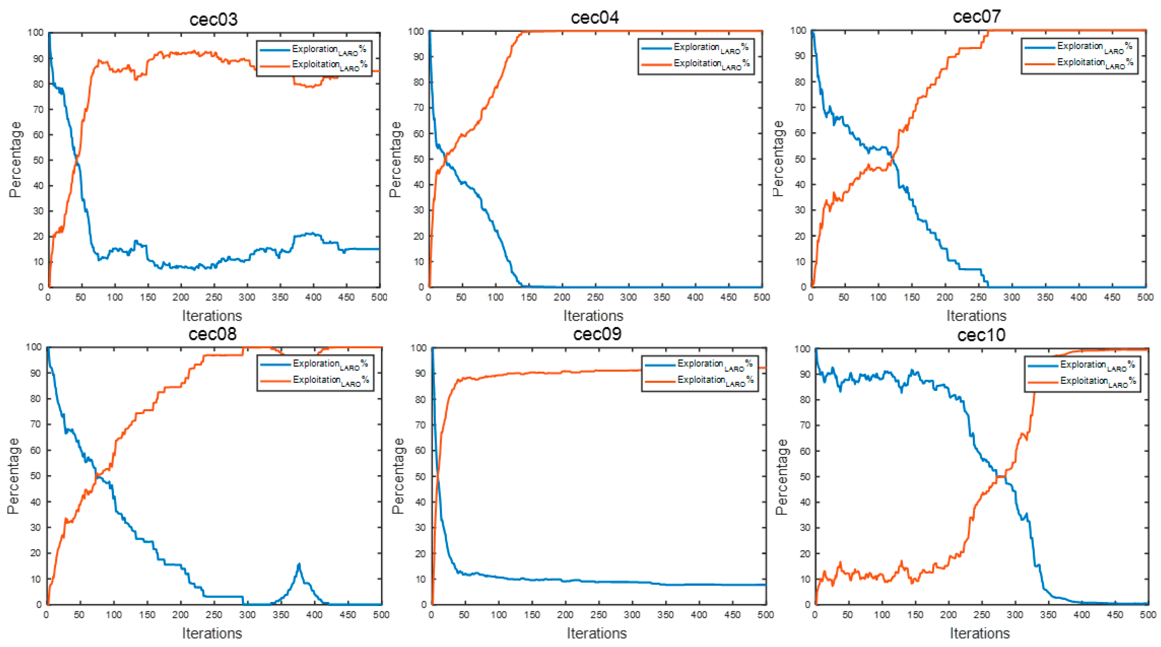
For the experimental part, we draw on the dimensional diversity metric suggested by Hussain et al. in [48] and calculate corresponding exploration and exploitation ratios. We selected the CEC2019 test set and provided the exploration and exploitation analysis graphs for some of the CEC2019 test functions in Figure 6.
From the figure, we can find that LARO starts from exploration in all the test functions and then gradually transitions to the exploitation stage. In the test functions of cec03 and cec09, we find that LARO can still maintain an efficient investigation rate in the middle and late iterations, and in the face of cec04, cec07, and cec08, LARO will quickly shift to an efficient discovery rate in the mid-term, ending the iteration with an efficient exploration situation. This discovery process shows that the more efficient exploration rate early in LARO guarantees a reasonable full-range finding capability to prevent getting stuck in current local solutions. In contrast, the middle step is smooth over the low, and the more efficient development rate in the later period guarantees that it can be exploited with higher accuracy after high exploration.
4.2. Comparative Analysis of Populations and Maximum Iterations
The population size and the maximum iterations affect the performance of the population-based metaheuristic algorithm. Therefore, in this section, we perform a sensitivity analysis of LARO involving the size of the initial population as well as the maximum iterations. This study considers the two most commonly used combinations of population and maximum iterations: (1) the size of artificial rabbit colonies is 50, and Tmax = 1000, (2) the size of artificial rabbit colonies is 100, and Tmax = 500, and LARO for the experiments conducted in case (1) is defined as LARO1, and LARO in case (2) is LARO2. The performance and running time of LARO1 and LARO2 are compared in the experiments with 23 test functions.
Table 2 provides a comparison of LARO with two different parameters in 23 benchmark functions. From the numerical results, it can be found that both parameters of ARO used almost similar running times. However, the convergence accuracy of LARO1 is better than that of LARO2, which indicates that LARO, with the case 1 parameter, can provide better convergence accuracy with the same guaranteed running cost. Therefore, the results show that the performance of LARO is affected by the population size and the number of iterations. The best performance was returned when the population size was set to 50, and the maximum number of iterations was 1000.
4.3. Analysis of Lévy Flight the Jump Parameter α
According to the mechanism of the Lévy flight strategy, we replace the r4 random numbers with the random numbers generated by the Lévy flight strategy. Thus, ARO is prevented from falling into local candidate solutions in the utilization phase. Additionally, the jump parameter α will affect the change of the updated position. In general, a larger jump parameter α, which increases the step size of the Lévy flight strategy, can ensure that the algorithm jumps out of the local solution, but it may also cause the optimal solution information not to be preserved. If the value is too small, it will affect the sensitivity of the Lévy flight strategy and, thus, the accuracy of the algorithm. Therefore, the jump parameter α has a great impact on the performance of LARO.
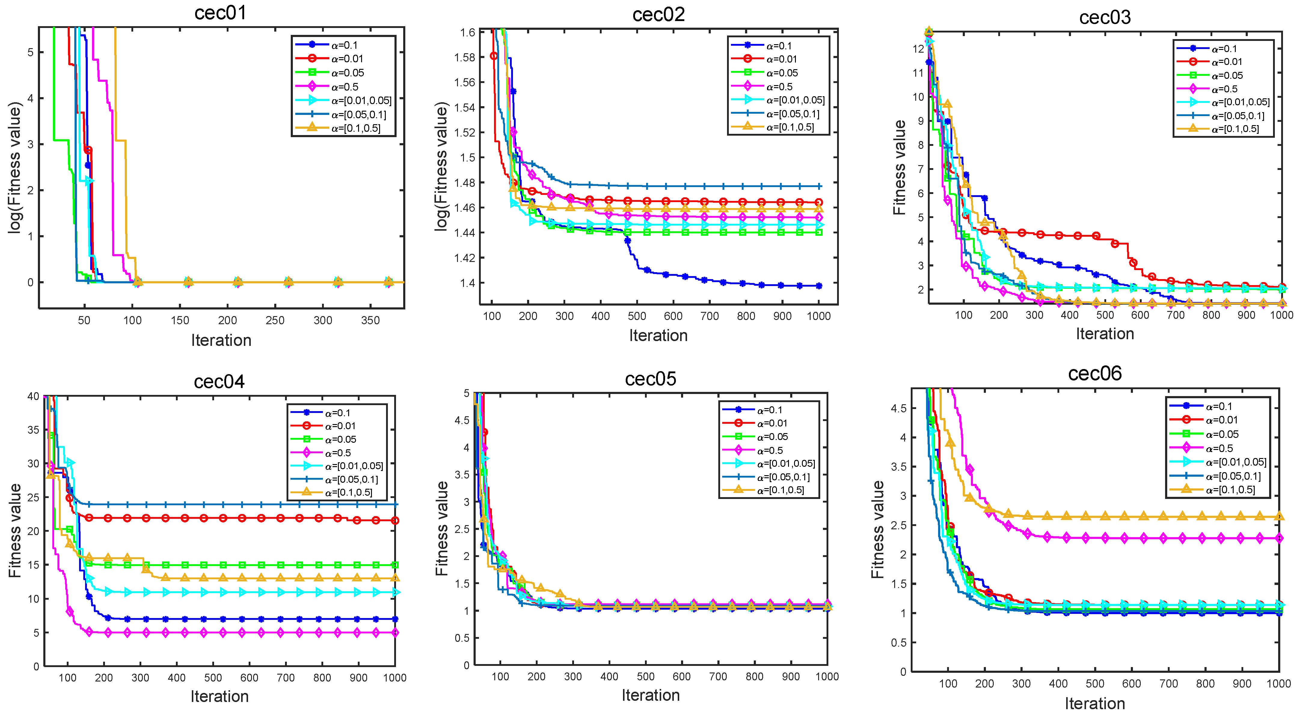
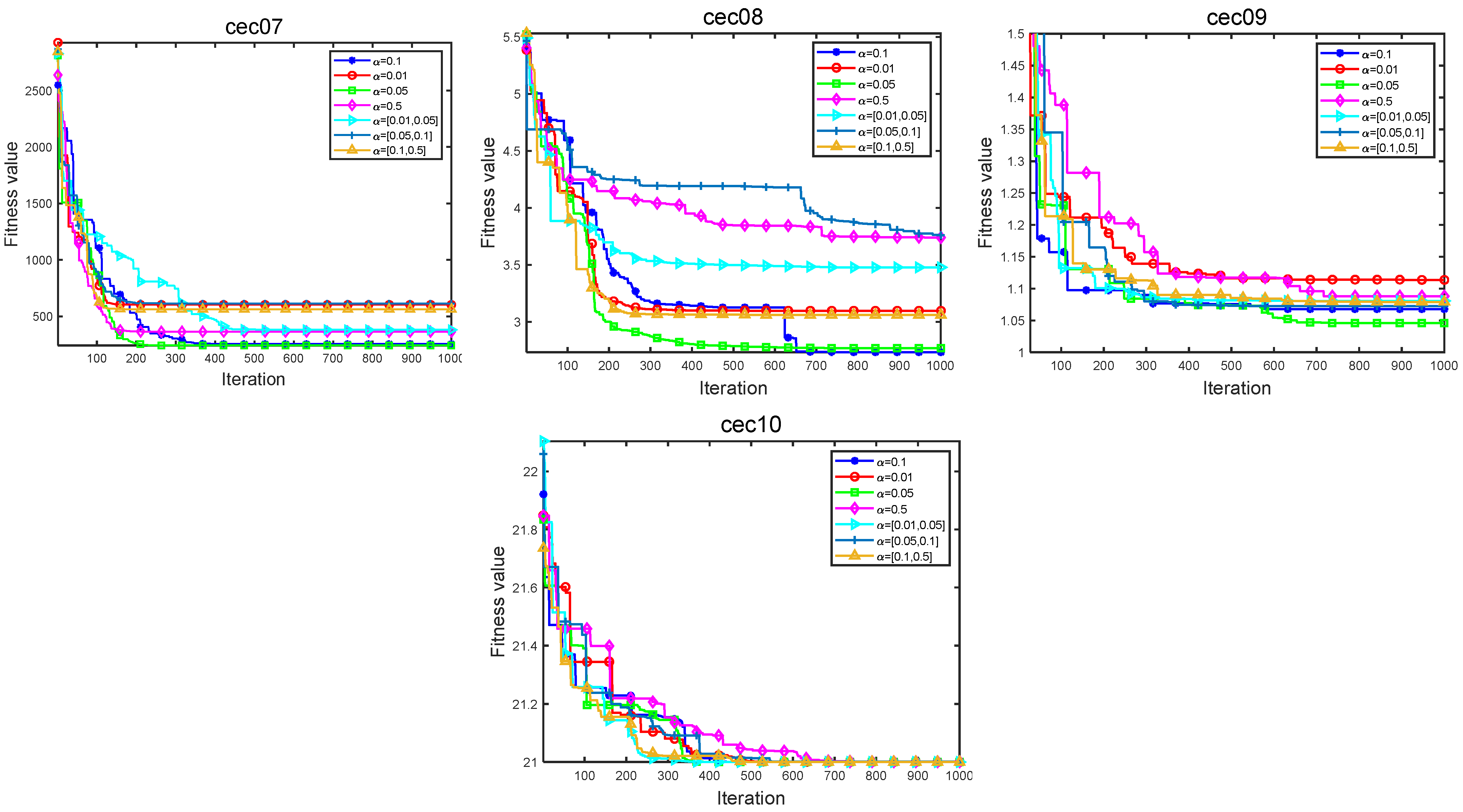
This section discusses the impact of the jump parameter α on the performance of the algorithm, and 10 test functions of CEC2019 are used to explore the impact of the jump parameter. The relevant jump parameters take four different values of 0.1, 0.01, 0.5, and 0.5, and three value intervals [0.01, 0.05], [0.05, 0.1], and [0.1, 0.5], respectively. The numerical intervals indicate the random number within each provided interval. The mean values of the solutions obtained by LARO for the CEC2019 test function over 20 independent trials are provided in Table 3. For a clearer view of the effect of the jump parameter α on LARO performance, Figure 7 provides the convergence curves for the ten test functions.
By analyzing Table 3, it can be observed that the average rank is the smallest when the jump parameter α = 0.1 at 3.2. and the best average values are obtained for five test functions (cec01, cec05, cec07, cec08, cec10). The value of the jump parameter α is a more in-between suitable value, indicating that the value balances the information of retaining the optimal solution and jumping out of the local solution. Figure 7 provides an iterative plot of the seven jump parameters. From the graph, it can be found that the LARO algorithm has a faster convergence rate, as well as a higher iteration accuracy for the jump parameter α = 0.1. Therefore, LARO can show the best performance when the jump parameter α is taken at 0.1.
4.4. Experiments on the 23 Classical Functions
To evaluate the strength of LARO in traversing the solution space, finding the optimal candidate solution, and getting rid of local solutions, we used 23 benchmark functions, where the unimodal test benchmarks (F1–F7) were used to examine the ability of LARO to develop accuracy. The multimodal benchmark set (F8–F13) was used to test the capability of LCAHA for spatial exploration. The fixed-dimensional multimodal test benchmarks (F14–F23) are mainly used to verify LARO’s excellent ability to handle low-dimensional spatial investigation. The dimensions of F01–F11 are 30, while the dimensions of F14–F23 are all different because they are fixed-dimensional multimodal test functions (the dimensions of F14–F23 functions are 2, 4, 2, 2, 2, 3, 6, 4, 4, 4, 4).
Table 4 shows LARO’s experimental and statistical results, the original ARO, and ten other search algorithms. Five relevant evaluation metrics (best, worst, average, standard, and ranking) were selected for this experiment. Additionally, we used Friedman ranking test results for all algorithms based on the mean value. In addition, the statistical presentation of the Wilcoxon test for LARO and other selected MH algorithms is shown in Table 4. When calculating the significance level, we let the default value of the significance level be set to 0.05. In addition, “+” denotes that a particular MH algorithm converges better than LARO. “−” denotes the opposite effect. “=” suggests that the impact of convergence in a given test problem is the same as the convergence of a particular MH algorithm.
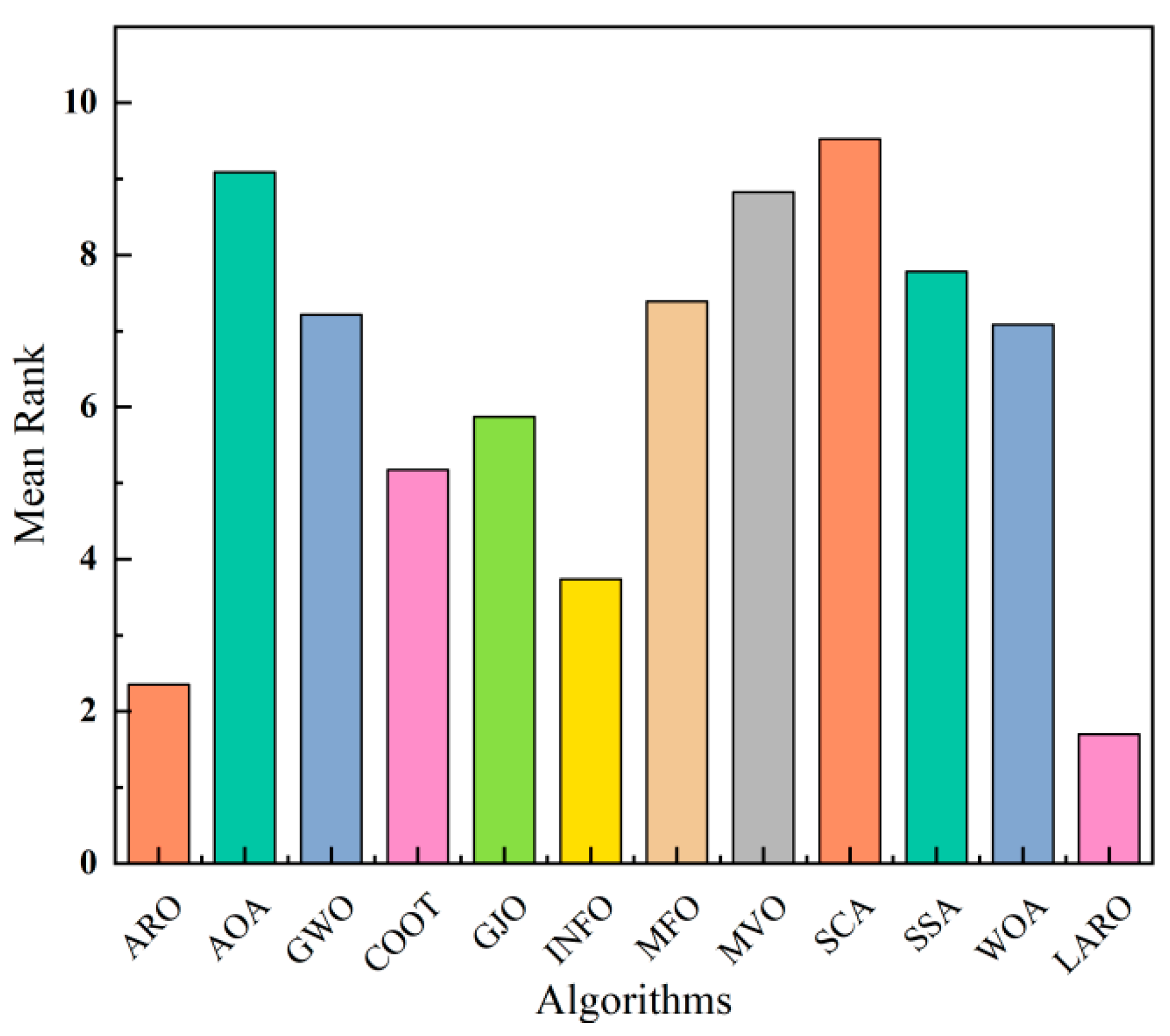
Analysis of the table shows that the proposed LARO has a Friedman rank of 1.6957 and is in the first place. Next is ARO, with 2.3478 ranked seconds. Figure 8 provides the average rank of the 12 comparison algorithms. LARO provides the best case among all algorithms on the 16 tested functions. In more detail, LARO ranked first in two unimodal functions (F1 and F3) and obtained the best results in four multimodal functions (F9, F10, F11, F13), respectively. Additionally, the best case was obtained in eight fixed-dimensional functions (F14, F16, F17, F18, F19, F20, F21, and F23). In addition to this, LARO shows strong competitiveness in some functions (F4, F8, F15, F22). Moreover, LARO and some other algorithms offer the best case when facing some of the tested functions. For example, ARO, GJO, INFO, and LARO obtain the best average solution when facing the F9 and F11 functions. In addition, ARO shows a notable ability to successfully solve three and seven problems in the face of unimodal and multimodal functions. Thus, it can be seen that LARO mainly improves the ability of the original algorithm to deal with unimodal problems while somewhat enhancing the ability to deal with multimodal and fixed-dimensional problems.
By analyzing the experimental results and tests, it can be seen that LARO improves the convergence ability of the algorithm by introducing a Lévy flight strategy in the random hiding phase, which leads to a good convergence effect and accuracy of LARO when facing unimodal problems without multiple solutions. In addition, due to the introduction of the selective opposition strategy in ARO, LARO can effectively filter the optimal solution among multiple local solutions when dealing with multimodal problems and fixed-dimensional problems. This result is because the selective opposition strategy helps the algorithm to jump out of the local solutions adaptively. Experimental results also demonstrate that LARO has better convergence than other algorithms and ARO when dealing with multimodal and fixed-dimension problems. Therefore, it can be shown that LARO is a reliable optimization method in terms of performance. However, it is also found that LARO tends to break the balance between exploration and exploration in the overall iterative process, affecting the algorithm’s performance.
In Table 5, we give the p-values of 11 MH algorithms, LARO algorithm, and the Wilcoxon test to check whether LARO outperforms other MH algorithms. The Wilcoxon test results for ARO, AOA, GWO, COOT, GJO, and INFO algorithms are 2/16/5, 1/1/21, 0/1/22, 0/11/12, 3/2/18, and 3/12/8. The Wilcoxon test results for MFO, MVO, SCA, SSA, and WOA were 1/5/17, 0/1/22, 0/1/22, 1/7/15, and 2/3/18, respectively.
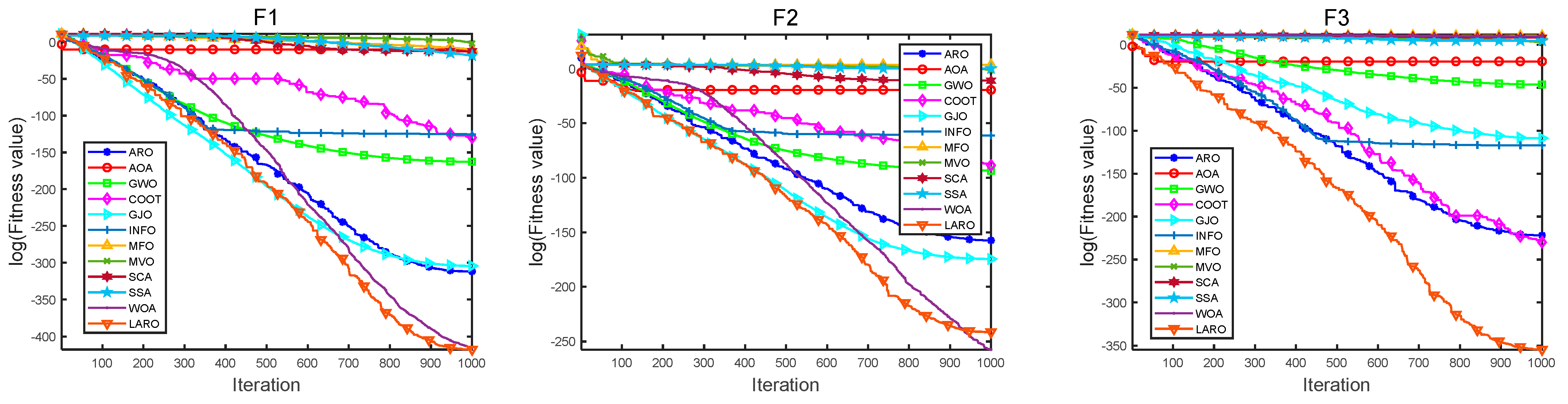
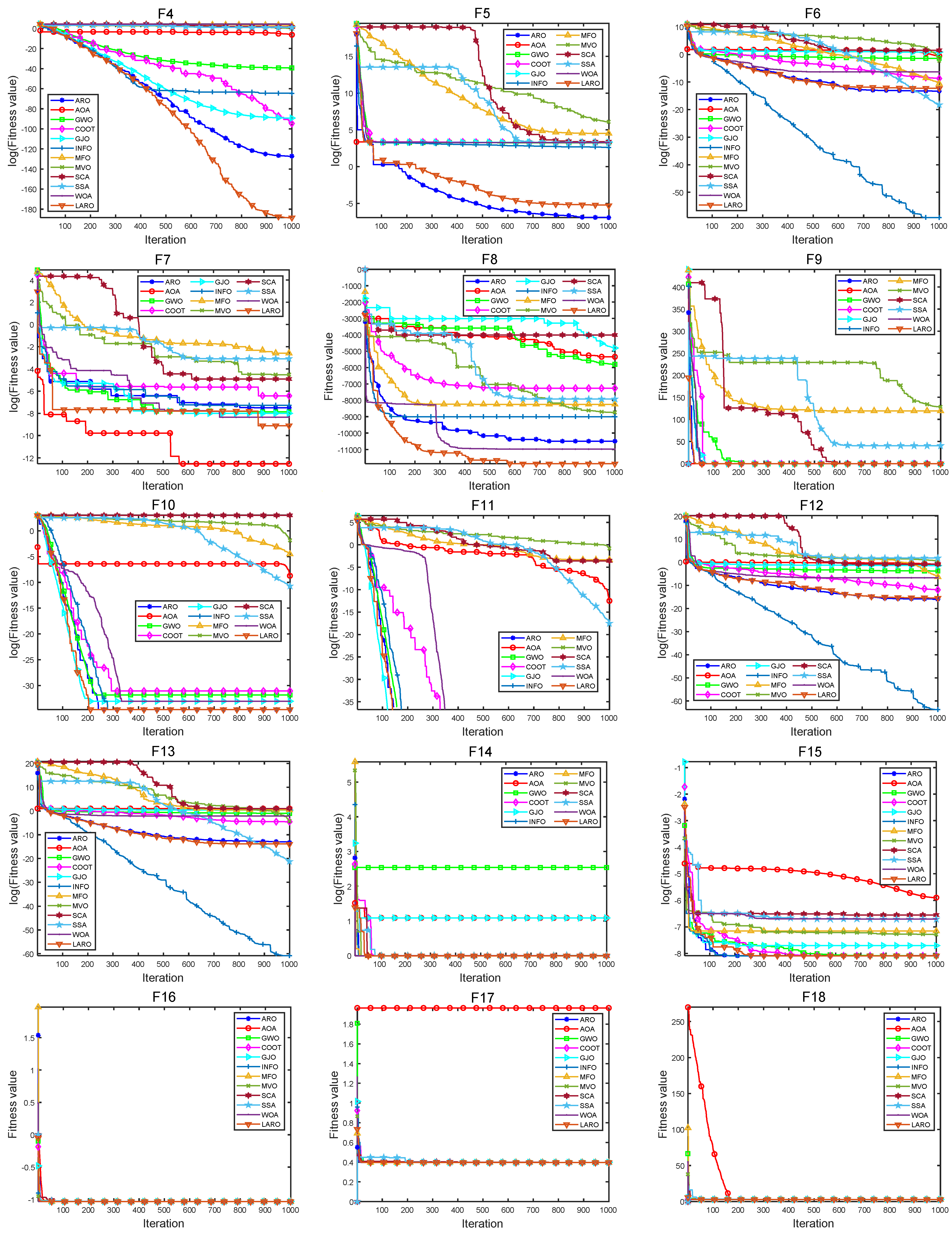
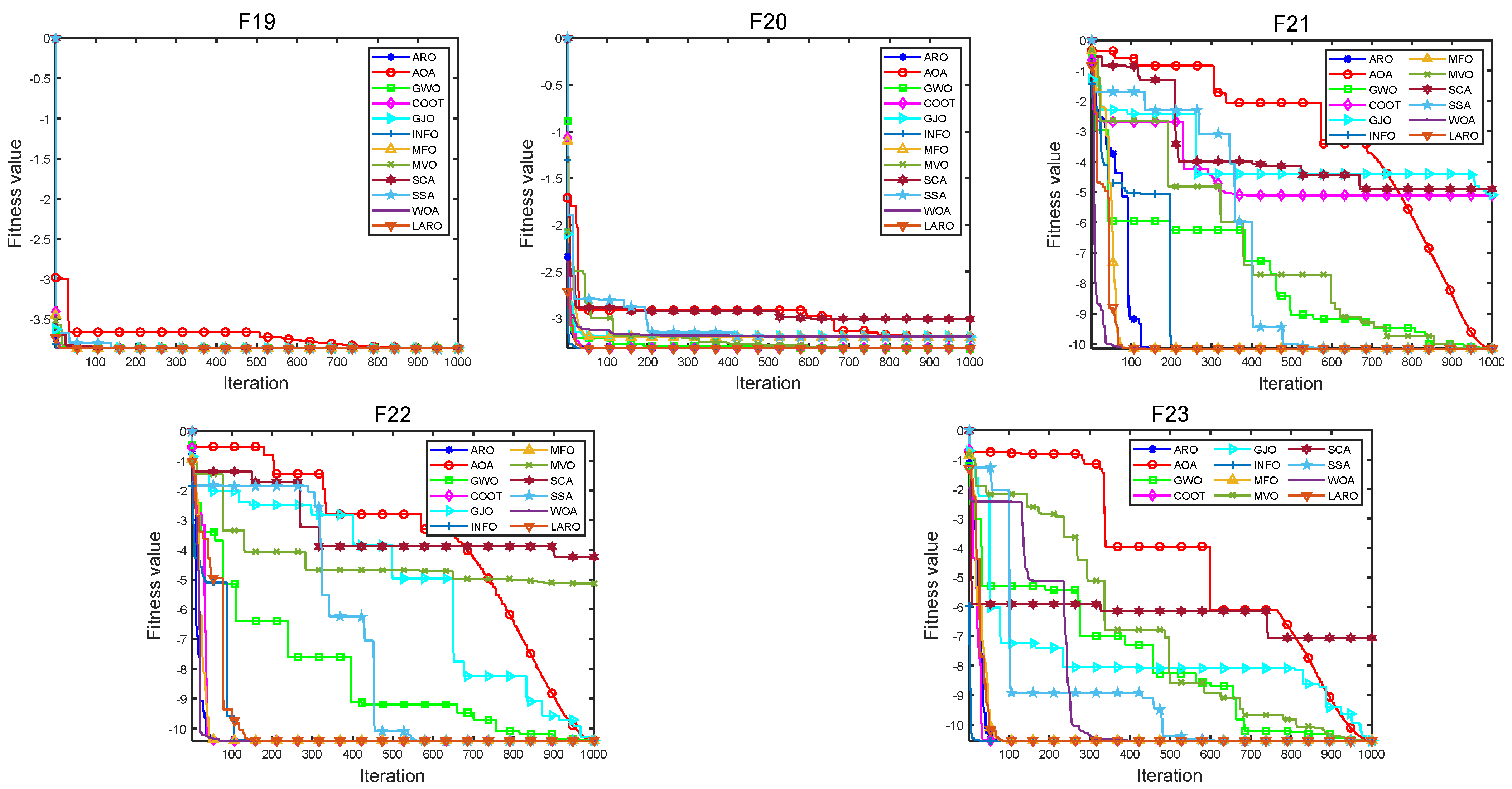
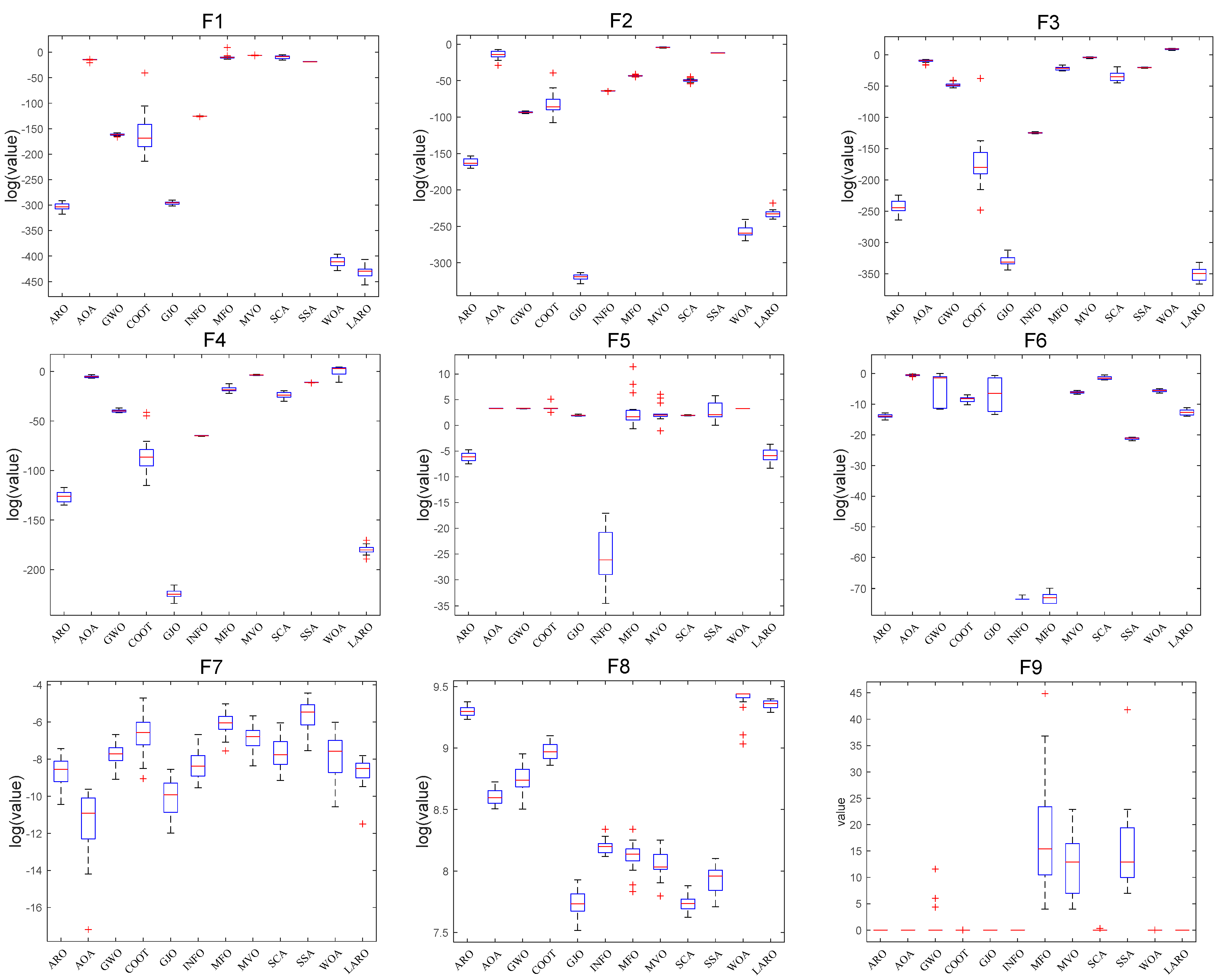
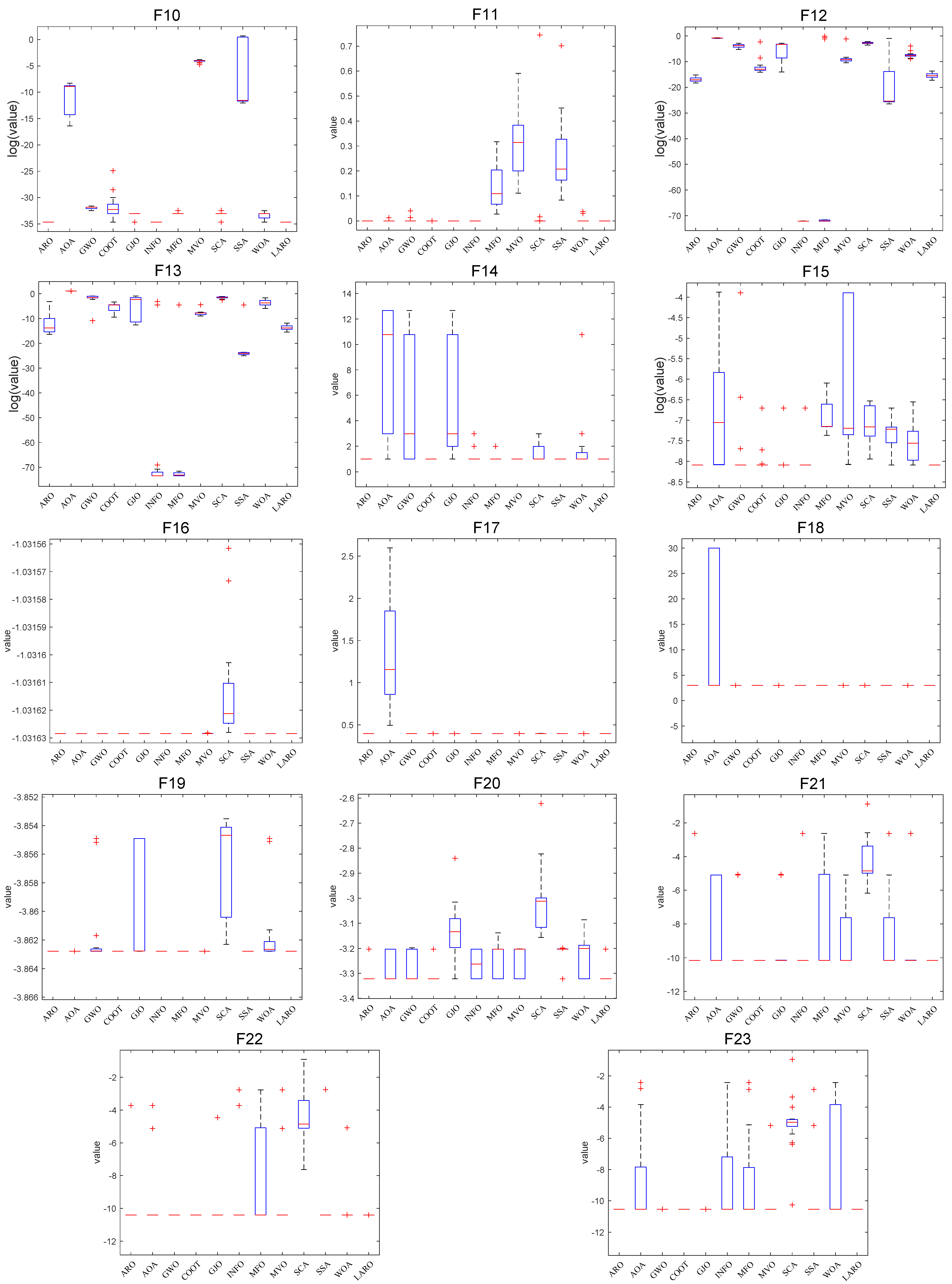
Figure 9 offers the convergence plots of the twelve different methods on the 23 benchmark functions, where the X-axis of the plot represents the iterations, and the Y-axis represents the degree of adaptation (some test functions (F1, F2, F3, F4, F5, F6, F7, F10, F11, F12, F13, F14, F15) are represented as logarithms of 10). The results in the figure demonstrate that LARO has a high-speed convergence rate and convergence accuracy when dealing with a part of the functions (F1, F2, F3, F4, F5) in the face of F1–F7 unimodal functions. Additionally, LARO continues to improve accuracy near the optimal solution later in the iteration. This analysis shows its reliable performance in getting rid of the local key. For the F8–F23 functions, we can see that LARO exhibits a characteristic that transitions rapidly between the early search and late development phases and converges near the optimal position at the beginning of the iteration. Then, LARO progressively determines the best marquee position and updates the answer to confirm the previous search results. Figure 10 illustrates box plots of 12 different MH algorithms for showing the distribution of means in various problems. In most of the issues tested, the distribution of LARO is more concentrated and downward than the other algorithms. This finding also illustrates the consistency and stability of LARO. Overall, LARO can handle the 23 basic test sets very well.
4.5. Experiments on the CEC2017 Classical Functions
In this section, the proposed LARO is simulated in CEC2017 for 29 of these test functions. LARO and the other comparison methods are executed 20 times individually, with the same relevant parameters set in Section 4.4. Cec01 and cec03–cec30 have a problem dimension of 10. Numerical results include the output of ARO [29], BWO [12], CapSA [13], GA [49], PSO [50], RSA [51], WSO [52], GJO [41], E-WOA [53], WMFO [54], and CSOAOA [26] outputs. As shown in Table 6, the evaluation methods of all 29 tested functions are compared by the proposed LARO algorithm. In addition, the results of Friedman’s statistical test are given in the last part of the table. In this case, Friedman’s statistical test ranking is given based on the mean value.
As shown in Table 6, the average rank of Friedman for LARO is 1.8621, while the average rank of WOS and ARO are 2.6897 and 2.7241, respectively. Therefore, LARO’s final ranking is the first. The results show that LARO provides a good output profile on 29 tested functions. LARO can succeed on 11 functions (cec05, cec07, cec09, cec11, cec15, cec17, cec18, cec20, cec22, cec23, cec28, cec30). In addition, LARO was able to obtain better optimization results and average values for the ten tested functions (cec01, cec03, cec06, cec08, cec10, cec14, cec19, cec21, cec27, cec29). The numerical results show that the proposed LARO exhibits excellent performance in the unimodal problem, indicating that the LARO algorithm again converges quickly. The performance of LARO for multimodal functions also illustrates that the introduced selective opposition effectively helps the algorithm to jump out of local solutions. In the face of composition and hybrid functions, LARO demonstrates excellent optimization ability, indicating the effectiveness of the Lévy flight strategy in improving the accuracy of the algorithm, while WSO and ARO can successfully solve six (cec01, cec08, cec10, cec12, cec13, cec29) and four functions (cec06, cec14, cec19, cec26), respectively.
4.6. Experiments on CEC2019 Test Functions
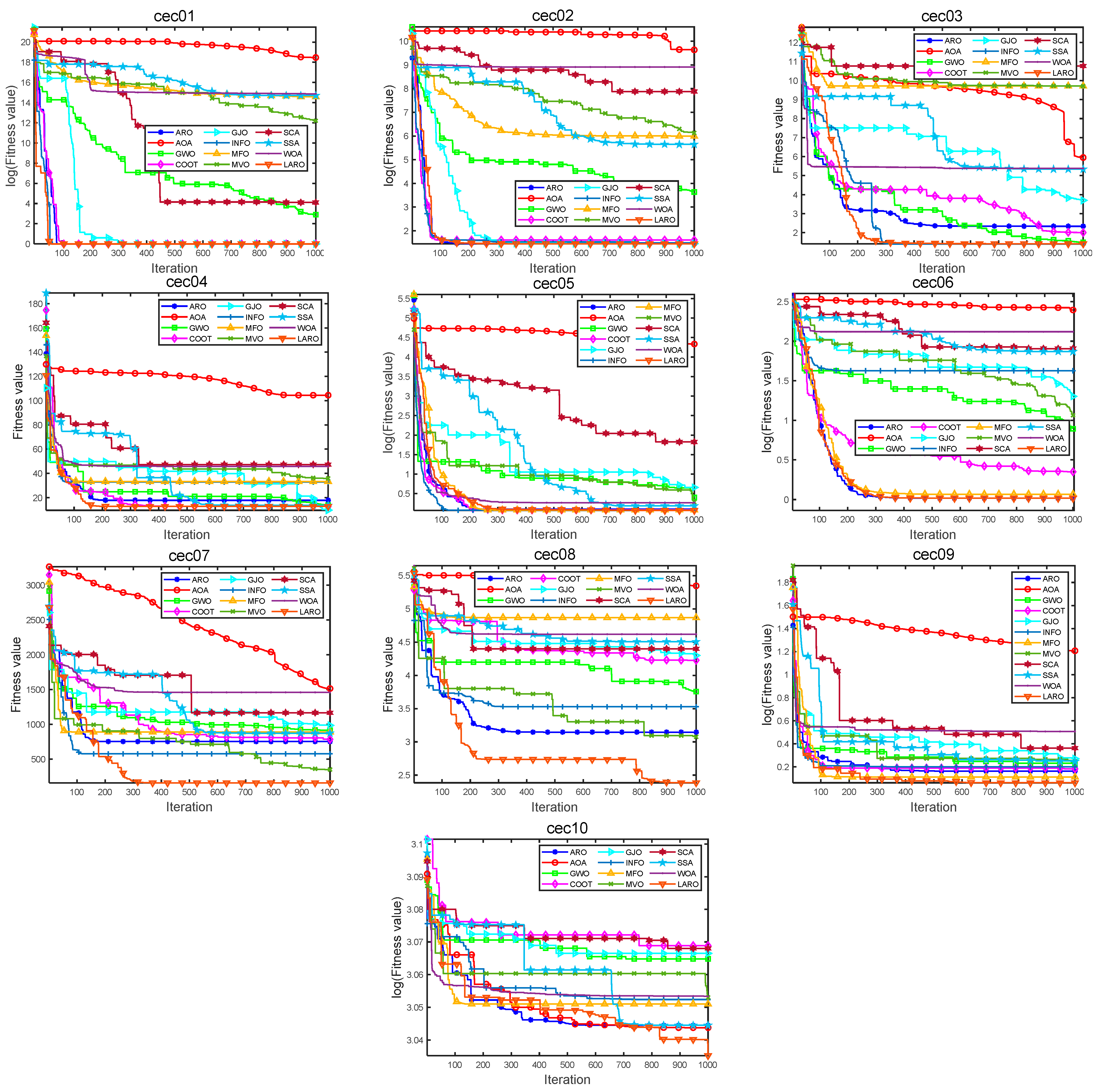
In this section, the proposed LARO has experimented with ten functions in CEC2019 [26]. The LARO algorithm is executed 20 times individually, and the parameters given are consistent with those of the numerical experiments in Section 4.3. Among them, the dimensionality of the functions cec01–cec03 is different from the others, with 9, 16, and 18 for cec01–cec03, respectively, while the problem dimensionality of cec04–cec10 is 10 [55]. The numerical results in agreement with AOA [38], GWO [39], COOT [40], GJO [41], INFO [42], MFO [43], MVO [44], SCA [45], SSA [46], WOA [47] are compared. As shown in Table 7, the four relevant evaluation methods are compared by the proposed LARO algorithm in all ten tested functions. In addition, the Wilcoxon and the Friedman statistical test results are given in the last part of the table. The experimental results conclude that LARO is superior in handling these challenging optimization function problems. LARO ranks first with an average ranking of 1.3636. In addition, LARO performs as the optimal case in seven of the ten CEC2019 functions (cec01, cec04, cec05, cec06, cec07, cec08, cec10), and ARO shows the best results in the other three functions (cec02, cec03, cec09). Numerical experimental results demonstrate that the LARO algorithm can accurately approach the optimal solution and is highly competitive with other MH methods for various types of problems. Moreover, experimental results likewise demonstrate that the LARO algorithm enhances the variety of the population and the accuracy of solving the problem due to the addition of the Lévy flight and the selective opposition, which effectively avoids local optimal solutions.
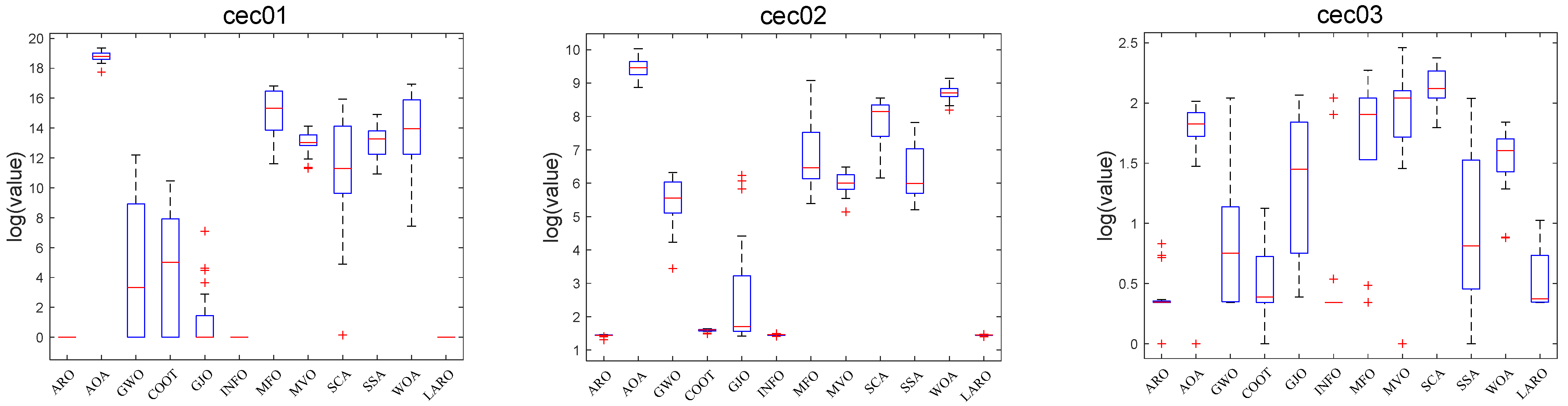
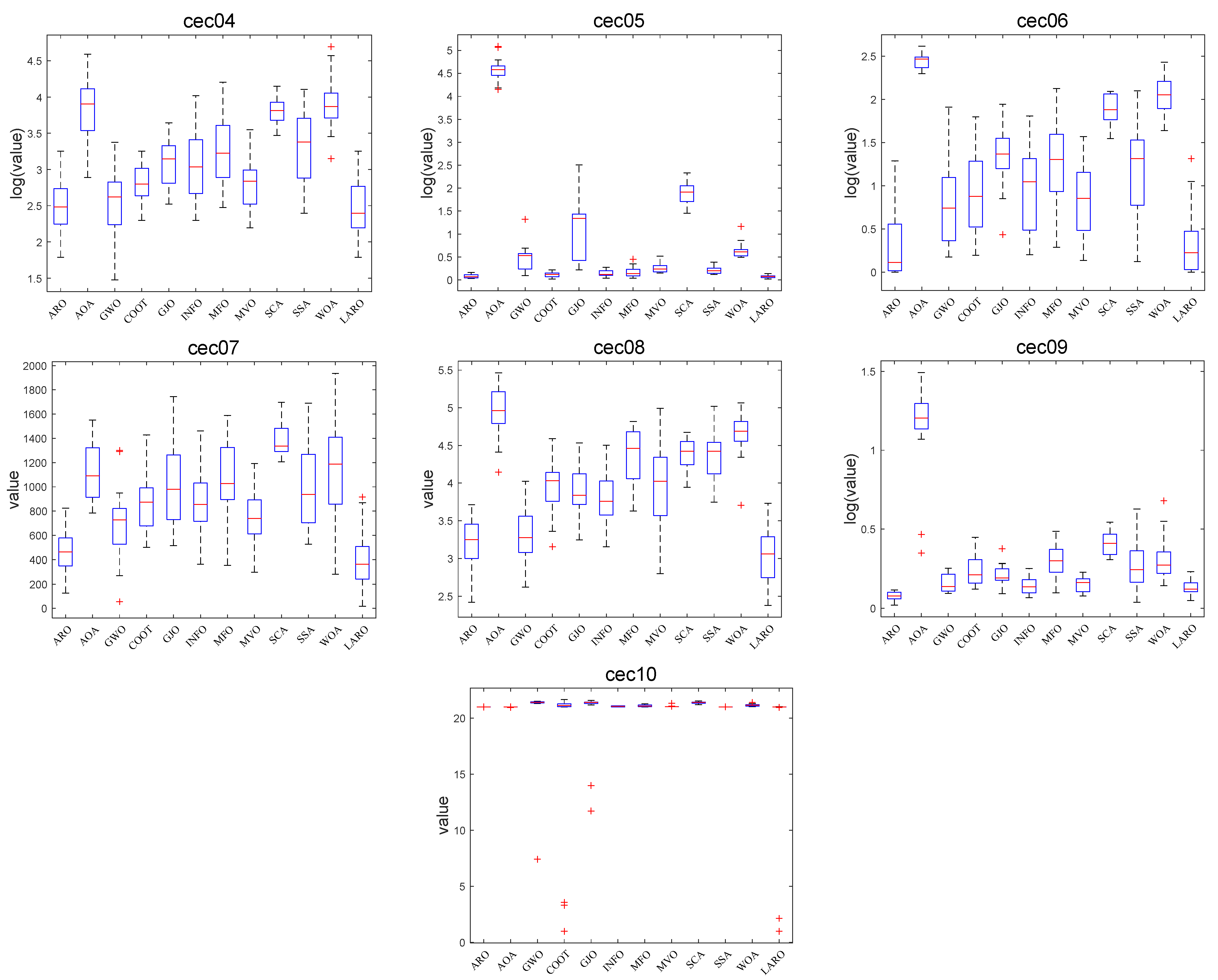
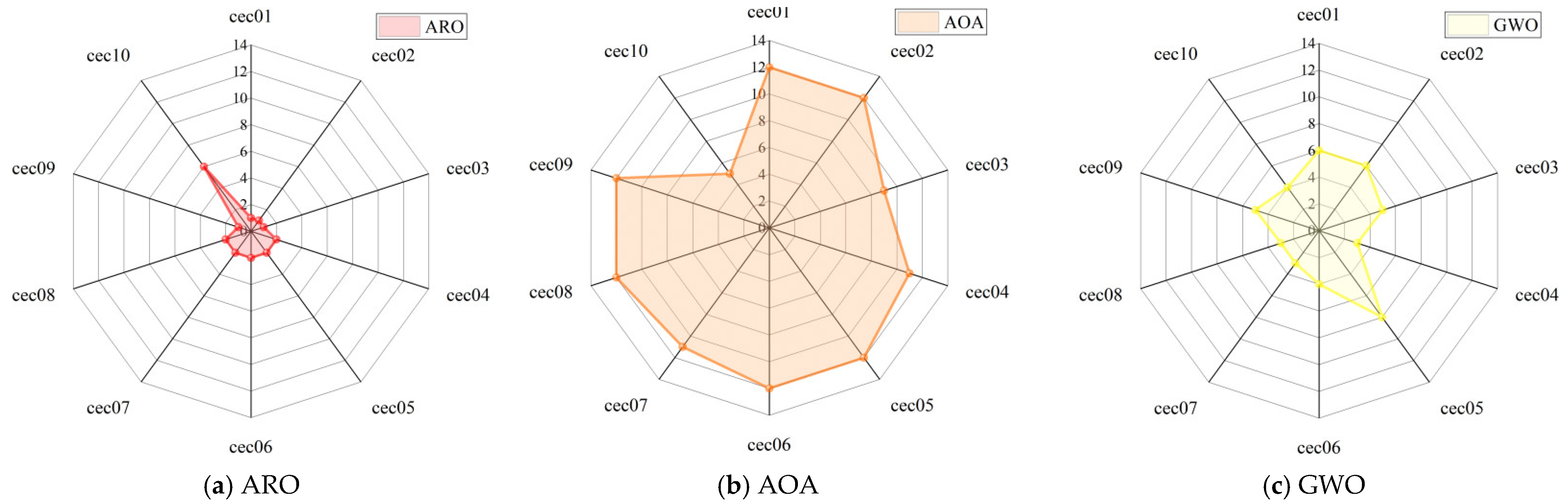
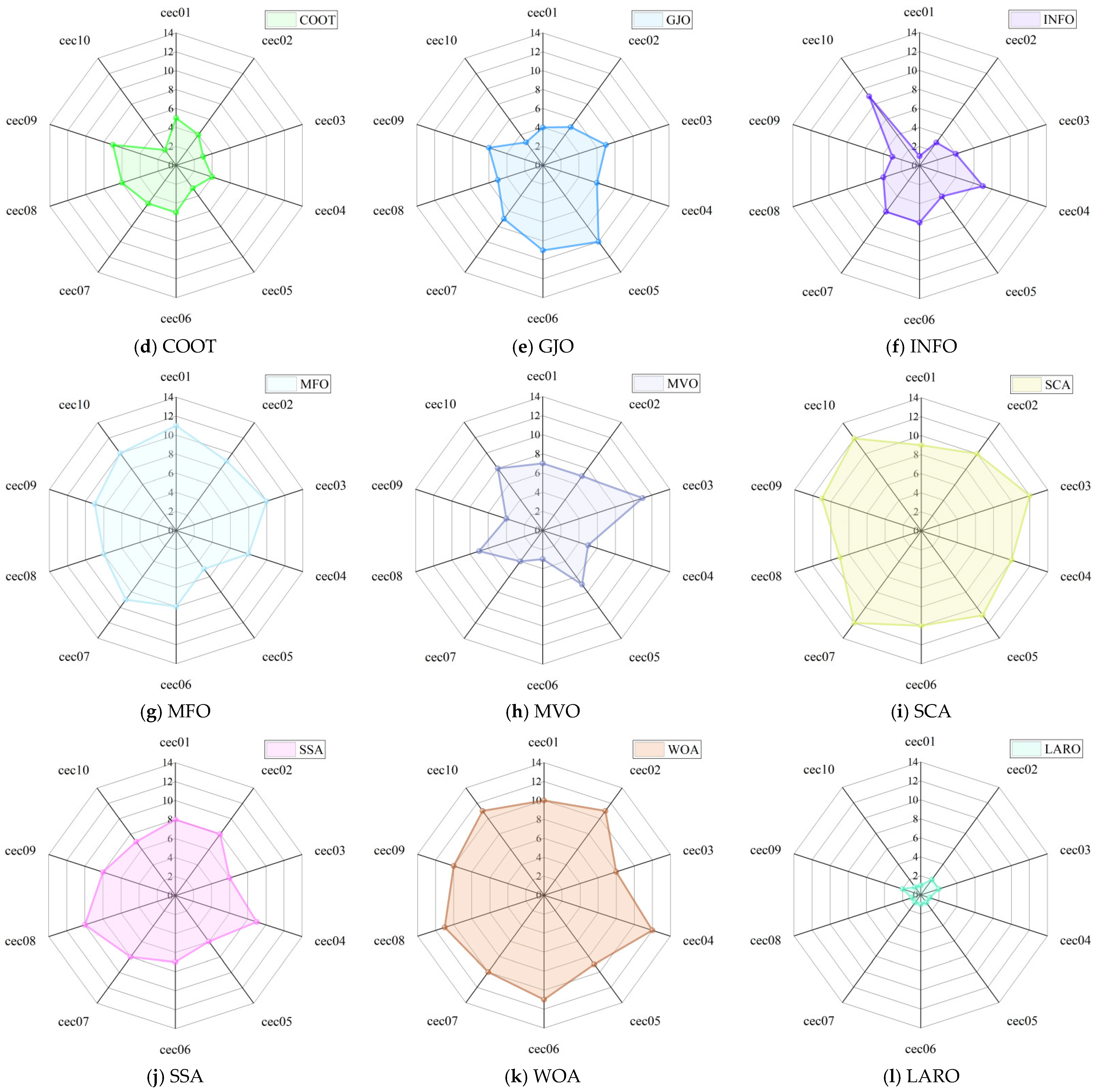
The convergence plots of the MH method in Figure 11 show the high quality and high accuracy of the LARO solutions and the significant convergence speed, such as cec01, cec02, cec03, cec04, cec05, cec06, cec7, cec08, cec10. Box plots and radar plots of the test function runs in CEC2019 are provided in Figure 12 and Figure 13, respectively, where these box-line plots provide very small widths, indicating the stability and superiority of LARO. In comparison, the radar plot demonstrates that LARO has the smallest ranking among all the tested functions. In Table 8, we give the p-values of 11 MH methods, the LARO algorithm, and the Wilcoxon test to check whether LARO outperforms other MH algorithms. The Wilcoxon test results for AROO, AOA, GWO, COOT, GJO, and INFO algorithms are 2/7/1, 0/0/10, 0/2/8, 0/1/9, 0/0/ The Wilcox test results for MFO, MVO, SCA, SSA, and WOA are 0/0/10, 0/1/9, 0/0/10, 0/1/9, and 0/0/10, respectively.
4.7. Impact Analysis of Each Improvement
The experiments in this section focus on numerical experiments of LARO with the compared algorithms on three standard test sets (23 benchmark test functions, CEC2017, CEC2019). This section summarizes the impact of different improvement strategies on the algorithm performance.
The introduction of the Lévy flight strategy in ARO is mainly used to solve the problem of low convergence accuracy of the original ARO. In contrast, single-peaked functions (e.g., F01–F07) are often used to test the convergence accuracy of the algorithm due to characteristics such as the absence of multiple solutions and the ease of exploration to the vicinity of the optimal solution. In the numerical experiments of 23 benchmark test functions, LARO ranks 1, 3, 1, 2, 3, 5, and 3 among the F01–F07 single-peaked functions, respectively. Except for F05–F06, the convergence accuracy of LARO is higher than that of the original ARO. In addition, in the numerical experiments of CEC2017, LARO ranks better than the original in both cec01 and cec03 ARO. Therefore, the Lévy flight strategy helps ARO to improve convergence accuracy successfully.
The selective backward learning strategy is introduced mainly to help ARO to jump out of the local solution in time. The multi-peaked functions (e.g., F08–F13, cec04–cec10 of CEC2017, and cec01–cec10 of CEC2019) are prone to fall into the vicinity of local solutions during the search process due to the existence of multiple solutions, which affects the convergence performance of the algorithm. Therefore, the algorithm’s ability to iterate over the multi-peaked functions reflects its ability to jump out of local solutions. In the numerical experiments with 23 benchmark test functions, LARO ranks 2, 1, 1, 1, 1, 3, and 1 for functions F08–F13, respectively. Except for F12, LARO’s optimization average is higher than the original ARO. In addition, LARO ranks 3, 1, 2, 1, 2, 1, 1, and 2 against cec04–cec10 of CEC2017, respectively. Except for cec06, the optimized average value of LARO is higher than that of the original ARO, and when facing the test set of CEC2019, the average ranking of LARO is 1.3636, which is higher than ARO at 1.9091. Therefore, LARO converges better than the original ARO when dealing with multi-peaked functions, which indicates that the selective backward learning strategy helps LARO to better jump out of the local solution.
5. Application of LARO in Semi-Real Mechanical Engineering
This subsection uses six practical mechanical engineering applications. There are many constraint treatments for optimization problems, such as penalty functions, co-evolutionary, adaptive, and annealing penalties [56]. Among them, penalty functions are the most used treatment strategy because they are simple to construct and easy to operate. Therefore, this paper uses the penalty function strategy to handle the optimization constraints of these six mechanical engineering optimization models, for the engineering optimization problem with minimization constraints defined as:
Minimize:
Subject to:
where m is the number of inequality constraints and k is the number of equation constraints. is the design variable of the engineering problem with dimension n. For the case with boundary constraints, a boundary requirement exists for all dimensional variables:
where lb and ub are the lower and upper bounds of the n-dimensional variable and n is the number of dimensions of the variable.
Therefore, the mathematical description of the engineering optimization problem after constraint weighting is
where α is the weight of the inequality constraint and β is the weight of the equation constraint. Considering the optimization process to satisfy the inequality and equation constraints, we require α and β to be large values. This paper sets them to 1 × 10⁵ [38]. Therefore, the objective function is severely penalized (the value of the objective function increases) when the optimization solution exceeds any constraint. This mechanism will allow the algorithm to avoid illegal solutions inadvertently computed during the iterative process.
LARO and all the comparison algorithms were executed 30 times. The relevant parameters were a maximum iteration of 1000 and a population size of 50. In addition, for the solution of the practical engineering applications, we used the same comparison algorithms as in the numerical experiments, including AOA [38], GWO [39], COOT [40], GJO [41], INFO [42], MFO [43], MVO [44], SCA [45], SSA [46], WOA [47].
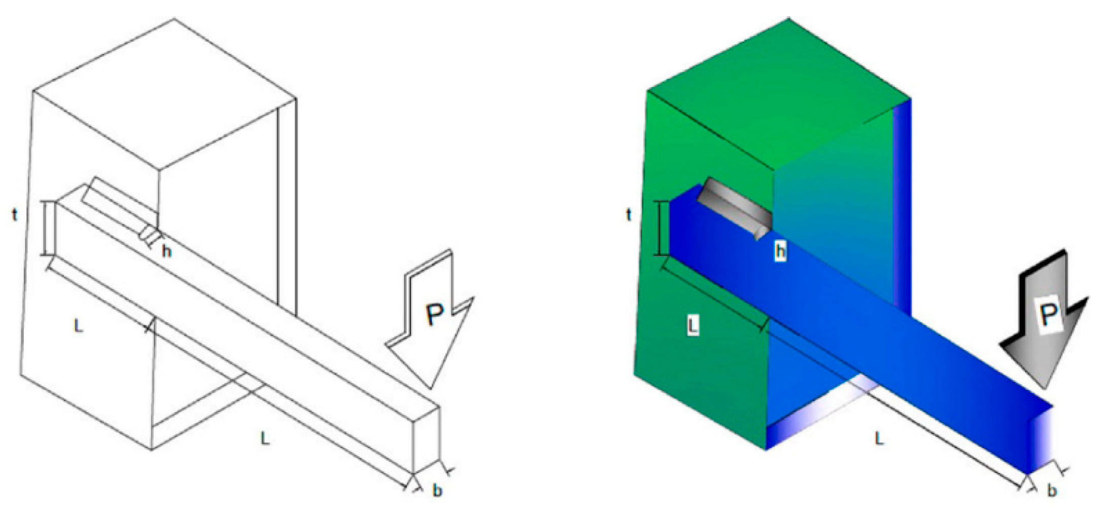
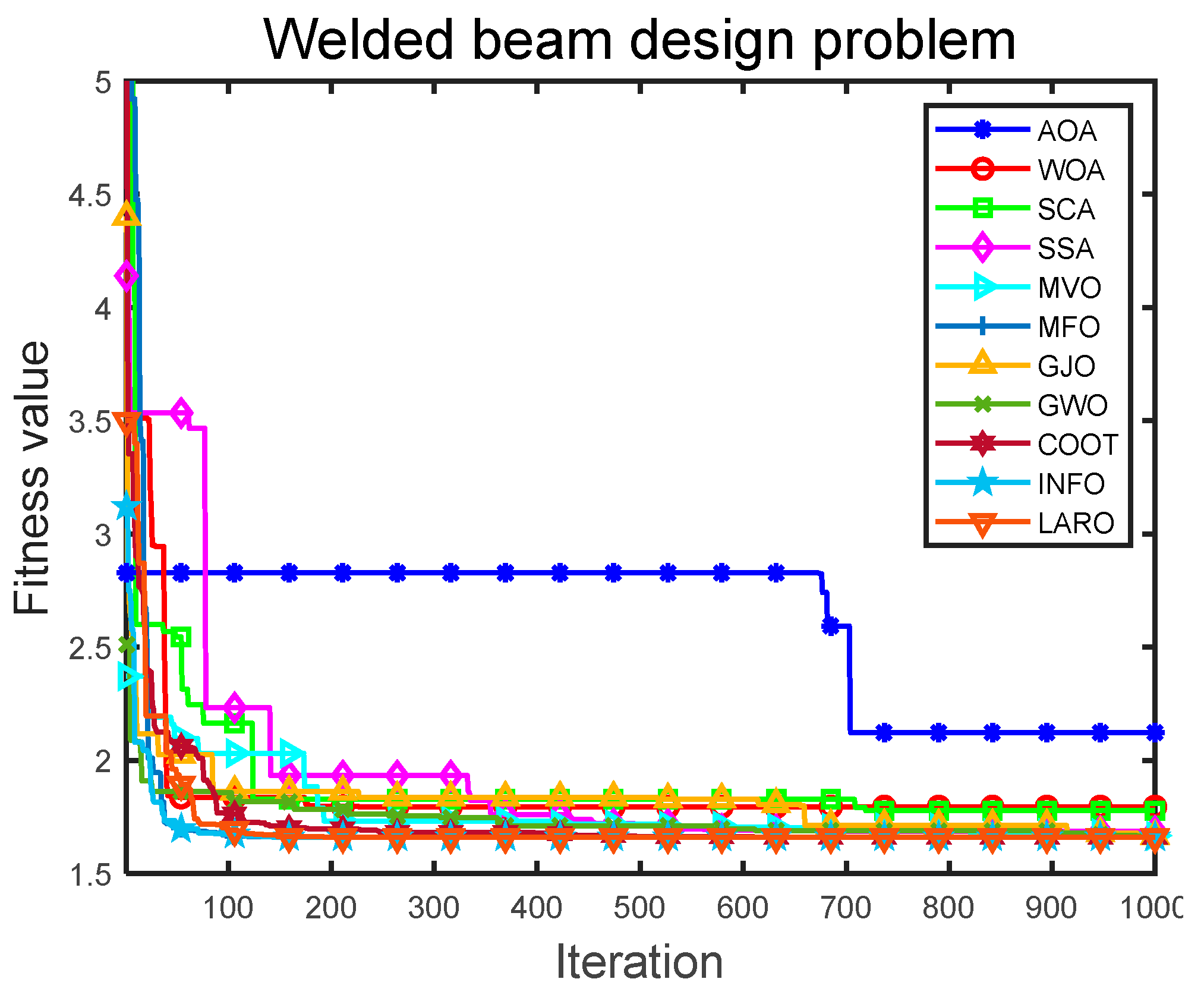
5.1. Welded Beam Design Problem (WBD)
The WBD requires that the design cost of the WBD be guaranteed to be minimal under various restraints. The schematic structural diagram of the WBD is provided in Figure 14. Four main relevant independent variables are obtained for the WBD: the welding thickness (h), rod attachment length (l), rod height (t), and rod thickness (b) [38]. The given variables are required to satisfy seven constraints. The model of the WBD is given below.
Minimize:
Variable:
Subject to:
where,
Table 9 provides the output results and best-fit cases for the search methods, and Table 10 documents the statistical output of the search methods. The combined evaluation of these two tables indicates that LARO obtained: the best outcomes for LARO with the same conditioning parameters. LARO has the best optimal value of the average. LARO obtains better results under the same conditioning parameters for the average and STD metrics, and, regarding the worst score metric, LARO performs well compared to different methods. The output results suggest that the LARO algorithm has good applicability for solving the WBD problem. Figure 15 provides the convergence iterations of LARO and the compared algorithms for the WBD problem. The figure shows that the proposed LARO has the best convergence and converges to the vicinity of the optimal solution in the early iterations. In comparison, the AOA has the worst convergence effect and convergence accuracy.
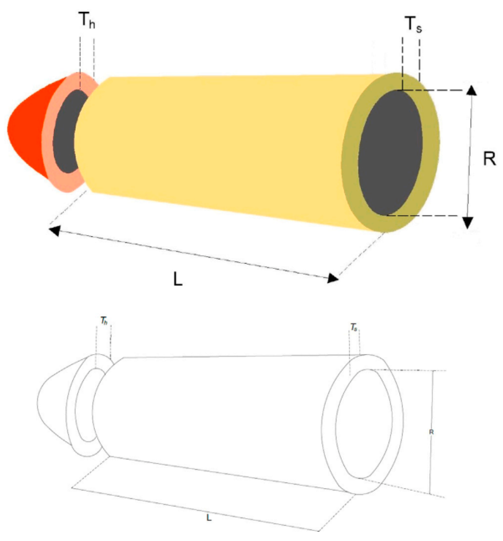
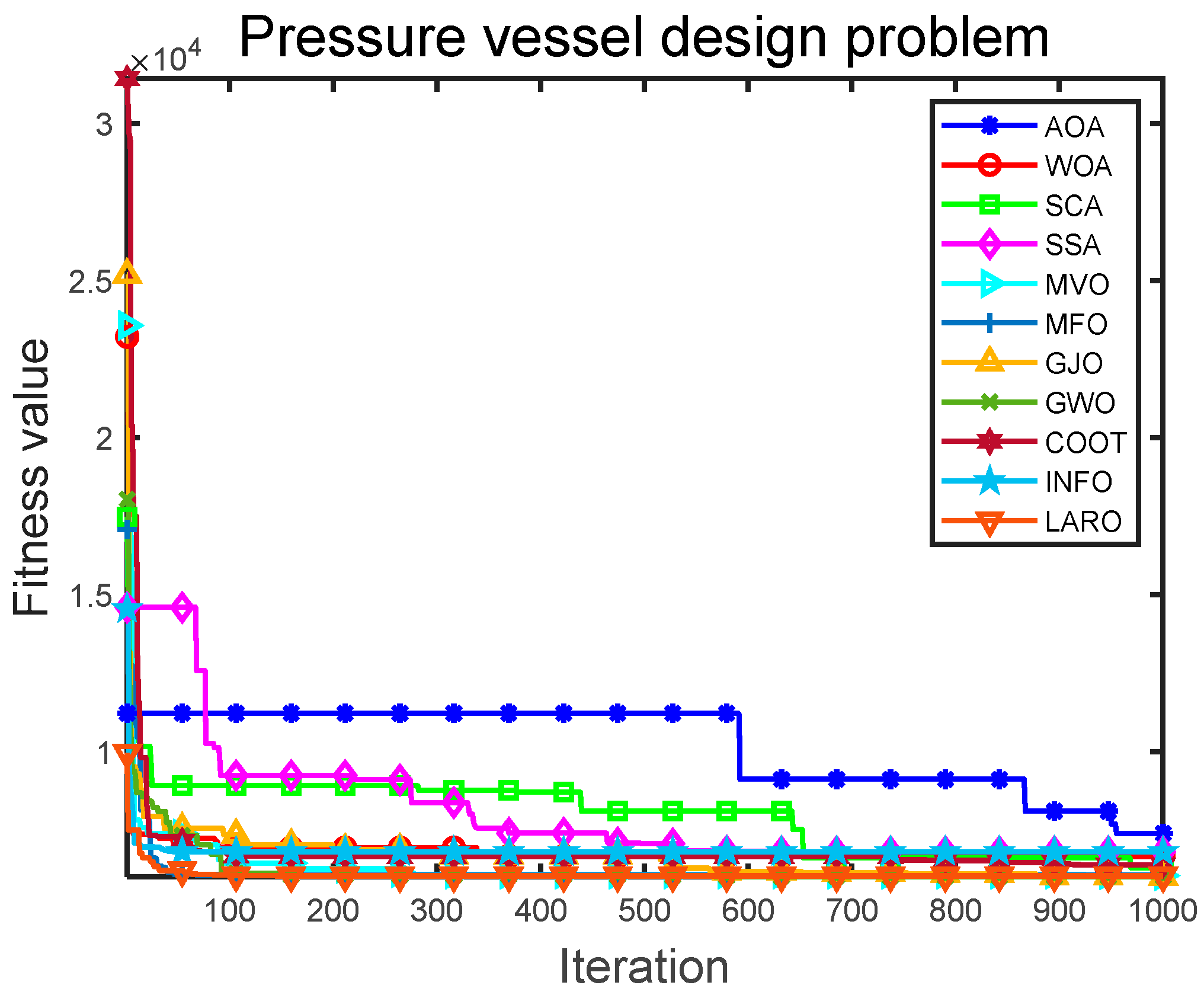
5.2. Pressure Vessel Design Problem (PVD)
The structure of the PVD is illustrated in Figure 16. The ultimate aim of the PVD is to keep the total cost of the three aspects of the cylindrical vessel to a minimum. Both edges of the vessel are capped while the top is hemispherical. The PVD has four relevant design variables, including the shell (Ts), the thickness of the head (Th), the radius of entry (R), and the length of the cylindrical section (L) [38]. The mathematical model (four constraints) of the PVD is presented as follows.
Minimize:
Variable range:
Subject to:
Table 11 provides the output results of the different search methods and the suitable average solution for solving the PVD problem. Table 12 documents the statistical outputs of the different methods of solving the PVD problem. By analyzing and evaluating two data, we find that LARO obtains suitable results for LARO with the same conditioning parameters. LARO has the suitable optimal value for the average value. LARO obtains the best case for the average and STD metrics compared to different search methods. The experimental output suggests that the LARO algorithm performs well in completing the PVD problem. Figure 17 provides the convergence iterations of LARO and the comparison algorithms in the PVD problem. From the results, it can be seen that LARO converges to the optimal solution. Compared to the other algorithms, LARO has the fastest convergence rate. SCA and SSA have poor convergence in the early stages, while AOA has poor convergence throughout. The results show that LARO has an advantage over the other algorithms in solving the PVD problem.
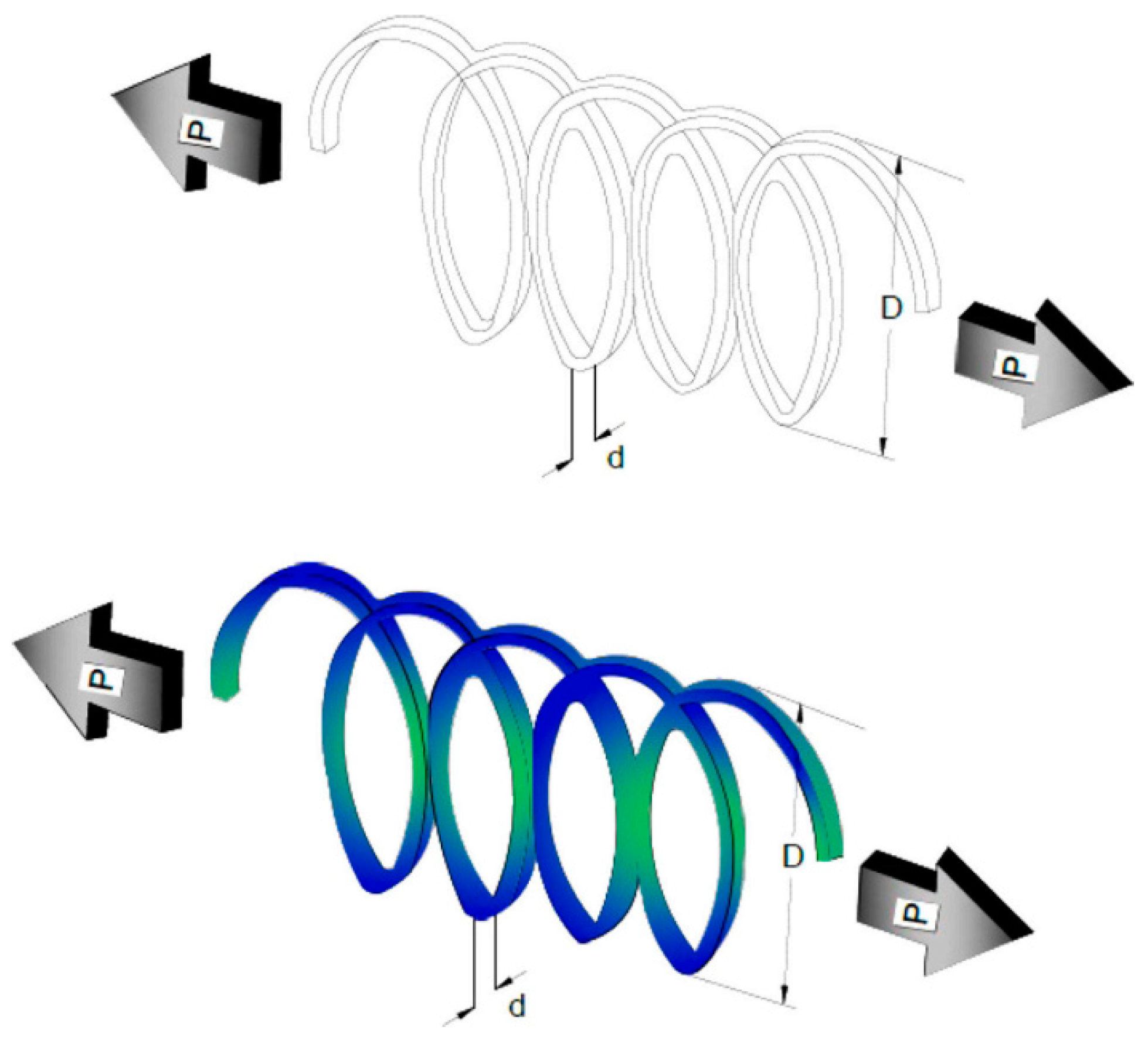
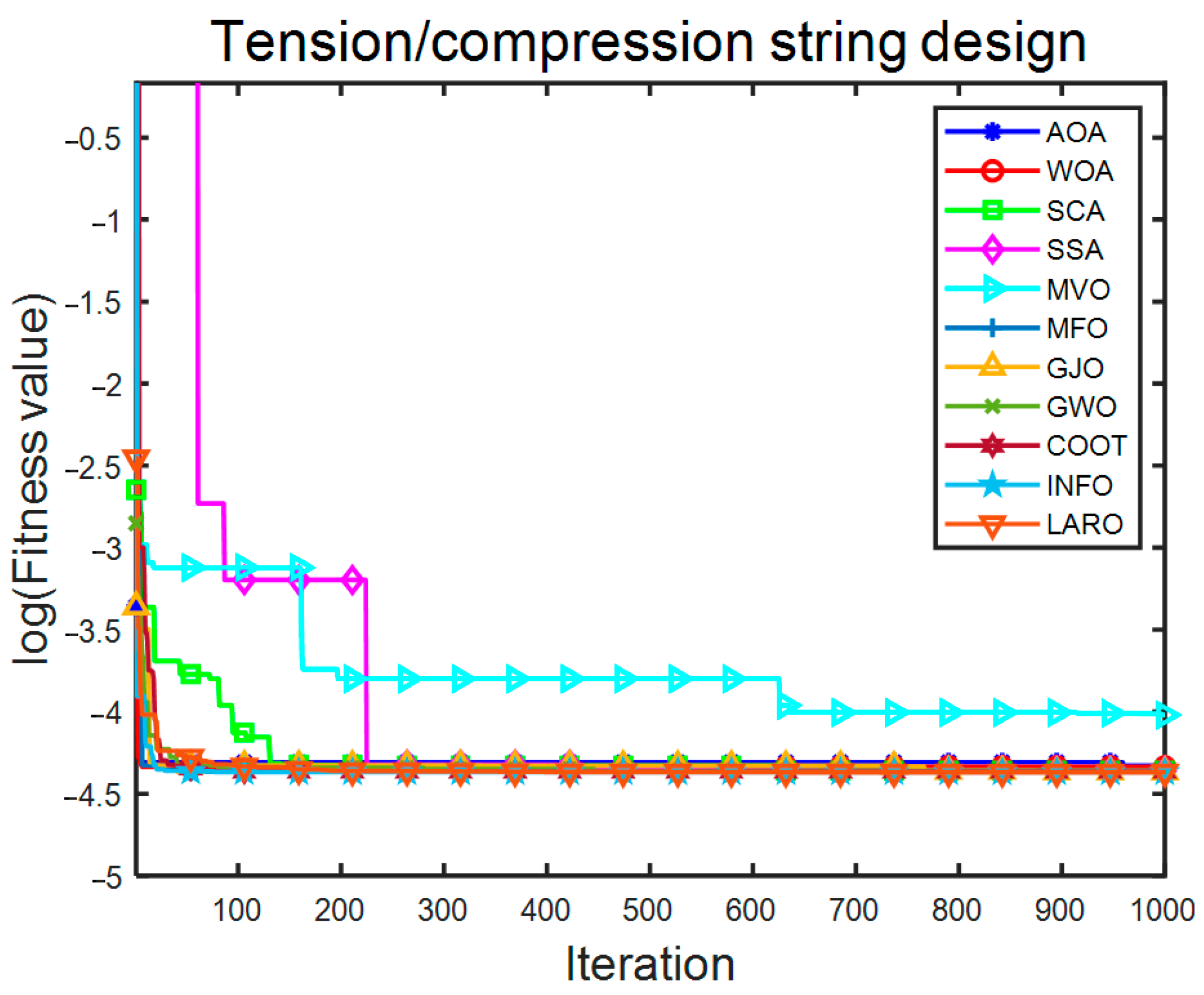
5.3. Tension/Compression String Design (TCS)
The most crucial objective of the TCS is to fit the mass optimally. The TCS includes three relevant design variables: wire diameter (d), number of active coils (N), and average coil diameter (D) [38]. A schematic representation of the TCS problem is displayed in Figure 18. The design model of the TCS is given below.
Minimize:
Variable range:
Subject to:
Table 13 provides the experimental results of all search methods and the best decision variables and the best average objective function values for solving the TCS problem, and provides the four constraint values for all algorithms, and Table 14 gives the statistical results for all search algorithms in solving the TCS problem. By analyzing and evaluating both data, we can find that LARO obtains better experimental results than other comparative algorithms. LARO has the best optimal, average, worst, and STD values. The numerical experimental results suggest that the LARO algorithm is a superior performance method for dealing with TCS. Figure 19 provides the convergence iterations of LARO and the comparison algorithms in the TCS problem. The vertical coordinates in the figure are the log values of the fitness values. From the results, it can be seen that LARO converges to the optimal solution. Compared to other algorithms, LARO has faster convergence. SSA has poor convergence in the early stage, while MVO has poor convergence throughout the process compared to different algorithms. The results show that LARO has an advantage over the other algorithms in solving the TCS problem.
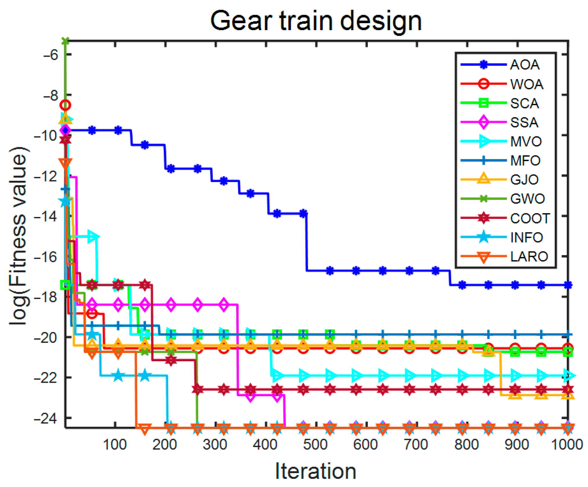
5.4. Gear Train Design (GTD)
The ultimate requirement of the GTD problem is to make the gear set with the most appropriate gear ratio cost to prepare the composite gear train. Figure 20 illustrates a schematic diagram of the GTD problem. There are four relevant integer variables for the GTD, where the four variables stand for the size of the teeth of four other gears [26]. These design variables represent the number of teeth on the gears and are denoted as Ta, Tb, Tc, and Td. The mathematical model of the GTD is given below.
Minimize:
Variable range:
Table 15 provides the experimental results for all search algorithms and the best average solution for the GTD problem. Table 16 presents the statistical output for the different search methods in solving the GTD. The analysis shows that LARO gives better experimental results compared to other search algorithms. LARO provides the best optimal, average, worst, and STD value. Numerical experiments show that the LARO algorithm can obtain good accuracy in solving the GTD problem. Figure 21 provides the convergence iteration results of LARO and the comparison algorithm on the GTD problem. The vertical coordinates in the figure are the log values of the adaptation values. From the results, it can be seen that LARO converges to the optimal solution. LARO’s convergence speed and accuracy are reasonable compared to other algorithms. SSA, GWO, INFO, and LARO all have good convergence, while AOA has poor convergence throughout the process compared to different algorithms. The results show that LARO has an advantage over other algorithms in solving the GTD problem.
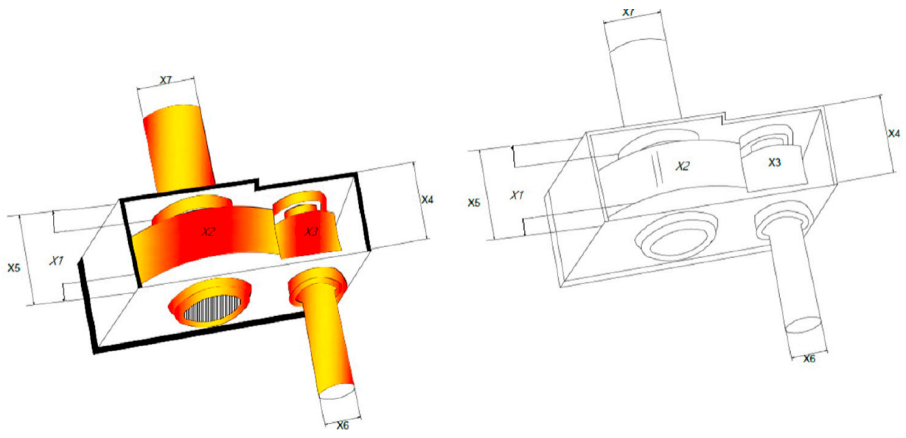
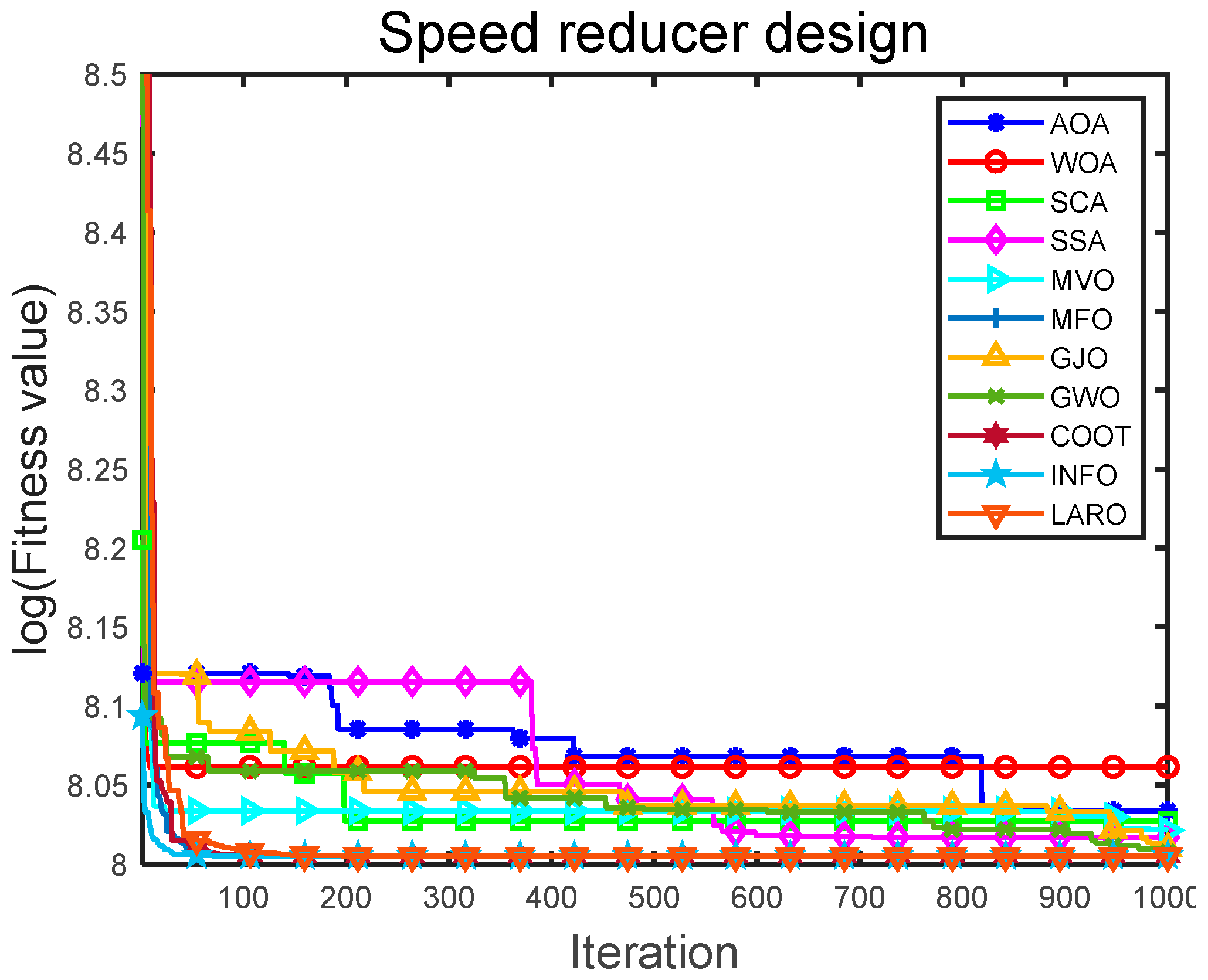
5.5. Speed Reducer Design (SRD)
The ultimate aim of the SRD is to ensure that the weight of the mechanical equipment is minimized while satisfying the 11 constraints. The schematic design diagram of the SRD is shown in Figure 22. The SRD has seven relevant variables, including the bending stress of the gear teeth, the covering stress, the transverse deflection of the shaft, and the stress in the shaft, used to control the facilities of the SRD problem [38]. Here, z1 is the tooth width, z2 is the tooth mode, and z3 is the discrete design variable representing the teeth in the pinion. Similarly, z4 is the length of the first axis between the bearings and z5 is the length of the second axis between the bearings. The sixth and seventh design variables (z6 and z7) are the diameters of the first and second shafts, respectively. The design model of the SRD (11 constraints and objective functions) is given below.
Minimize:
Variable range:
Subject to:
Table 17 shows the most suitable outputs from LARO and the different selection comparison methods in dealing with the SRD problem. Table 18 gives the statistics of all search algorithms. It can be found that LARO outperforms the different search algorithms in terms of optimal performance. LARO has the best optimal, worst, average, and STD values for the same maximum iterations, while the smaller STD also indicates that LARO has good robustness. Therefore, LARO is effective in optimizing SRD solutions. Figure 23 provides the results of the convergence iterations of the LARO and comparison algorithms on the SRD problem. The vertical coordinates in the figure are the log values of the adaptation values. From the results, it can be seen that LARO converges to the optimal solution. The convergence speed and convergence accuracy of LARO are good compared to other algorithms. All the algorithms converge to near the optimal solution in the early iteration. The results show that LARO is an excellent algorithm for solving the SRD problem.
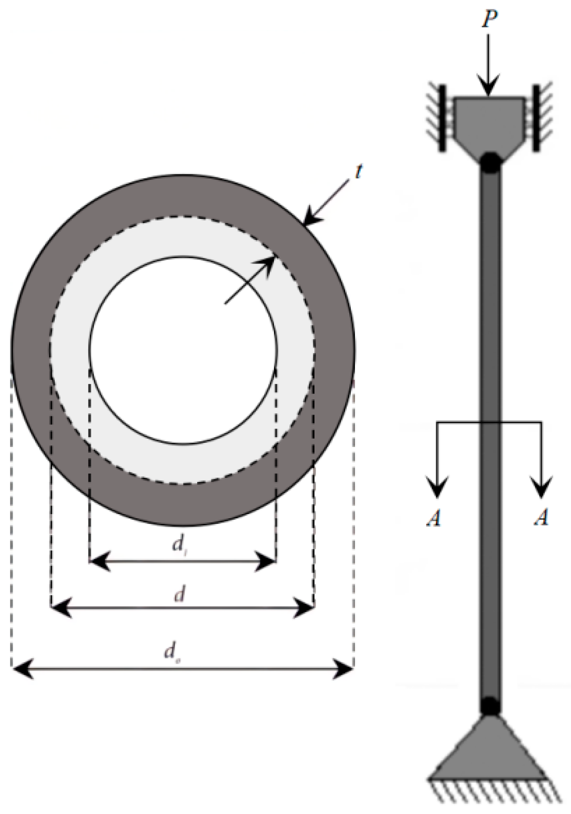
5.6. Tubular Column Design (TCD)
The TCD problem is to ensure that the cost of designing a homogeneous column with a tubular cross-section is minimized under the condition that six constraints are satisfied with suitable compressive loads [4]. The schematic design diagram of the TCD is illustrated in Figure 24. Two material-related conditions to be established for the TCD problem include yield stress σy = 500 kgf/cm2 and modulus of elasticity E = 0.85 × 10⁶ kgf/cm2. The mathematical model of the TCD problem is given below.
Minimize:
Variable range:
Subject to:
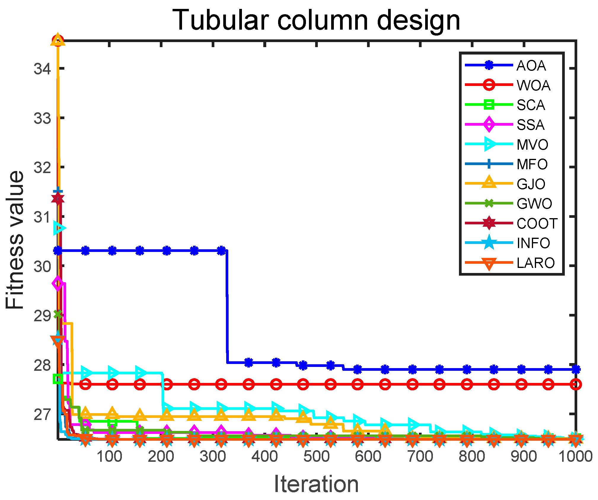
Table 19 presents the most suitable outputs obtained by the LARO and other selection comparison algorithms for the TCD problem. Table 20 gives the statistics of all search algorithms dealing with the TCD. It can be noticed that LARO outperforms the different search methods in terms of optimal performance. LARO has the best optimal, worst, average, and STD values for the same maximum iterations, while the smaller STD also indicates that LARO has good robustness. Therefore, LARO is effective in optimizing the solution of TCD problems. Figure 25 provides the results of the convergence iterations of the LARO and comparison algorithms on the TCD problem. From the results, it can be seen that LARO converges to the optimal solution. LARO converges faster compared to the other algorithms. MVO converges poorly in the early stages, while AOA and WOA converge poorly throughout the process compared to the different algorithms. The results show that LARO has an advantage over the other algorithms in solving the TCD problem.
6. Conclusions
In this study, an effective metaheuristic method called the enhanced ARO algorithm (LARO) is proposed. LARO is a variant of the ARO algorithm. To boost the global finding ability of ARO, the avoidance of local solutions and international exploration of LARO are designed by making full use of the Lévy flight strategy. In addition, local exploitation of LARO is achieved by using the selective opposition strategy. The most remarkable feature of LARO is that it has a straightforward structure and high computational accuracy, often requiring only the basic parameters (i.e., population size and termination conditions) for solving optimization problems. We tested the performance of LARO with 23 test functions, the CEC2019 test suite, and six mechanical engineering design problems. The experimental results show that LARO can obtain the optimal average solution in 16 of the 23 classical test functions and obtain the smallest average rank (2.3478). Additionally, LARO obtains the best solutions for five and seven functions in CEC2017 and CEC2019, respectively. The conclusion shows that the strategies for improved ARO are very effective in improving the optimization performance. However, there is still room for further improvement in the exploration ability of LARO when facing the CEC2017 test functions. In the mechanical optimization problem, all six practical problems are complex problems with multiple nonlinear constraints and multiple local solutions, and the output results show that LARO can obtain the best decision variables and objective function values. Because of its excellent convergence, exceptional exploration ability, and lack of need to fine-tune the initial parameters, LARO has excellent potential to handle optimization problems with various characteristics.
In future work, this study will expand the versions of the ARO algorithm to include the ARO algorithm for opposing learning initialization, the multi-objective ARO algorithm, the binary ARO algorithm, and the discrete version of the ARO algorithm [57,58,59,60,61,62]. In addition, we will focus on applying LARO to various complex real-world engineering optimization problems, such as hyperparametric optimization of machine learning algorithms, urban travel recommendations in intelligent cities, job-shop scheduling problems, image segmentation, developable surface modeling [63], and smooth path planning for mobile robots.
Author Contributions
Conceptualization, Y.W. and G.H.; Data curation, Y.W., L.H. and G.H.; Formal analysis, L.H. and J.Z.; Funding acquisition, G.H.; Investigation, Y.W., L.H. and J.Z.; Methodology, L.H., J.Z. and G.H.; Project administration, Y.W., J.Z. and G.H.; Resources, Y.W. and G.H.; Software, Y.W., L.H. and J.Z.; Supervision, G.H.; Validation, J.Z. and G.H.; Visualization, G.H.; Writing–original draft, Y.W., L.H., J.Z. and G.H.; Writing—review & editing, Y.W., L.H., J.Z. and G.H. All authors have read and agreed to the published version of the manuscript.
Funding
This work is supported by the Research Fund of Department of Science and Department of Education of Shaanxi, China (Grant No. 21JK0615).
Institutional Review Board Statement
Not applicable.
Informed Consent Statement
Not applicable.
Data Availability Statement
All data generated or analyzed during this study were included in this published article.
Conflicts of Interest
The authors declare no conflict of interest.
References
- Zhao, W.; Wang, L.; Mirjalili, S. Artificial hummingbird algorithm: A new bio-inspired optimizer with its engineering applications. Comput. Methods Appl. Mech. Eng. 2022, 388, 114194. [Google Scholar] [CrossRef]
- Zamani, H.; Nadimi-Shahraki, M.H.; Gandomi, A.H. Starling murmuration optimizer: A novel bio-inspired algorithm for global and engineering optimization. Comput. Methods Appl. Mech. Eng. 2022, 392, 114616. [Google Scholar] [CrossRef]
- Knypiński, Ł. Performance analysis of selected metaheuristic optimization algorithms applied in the solution of an unconstrained task. COMPEL—Int. J. Comput. Math. Electr. Electron. Eng. 2021, 41, 1271–1284. [Google Scholar] [CrossRef]
- Agushaka, J.O.; Ezugwu, A.E.; Abualigah, L. Dwarf Mongoose Optimization Algorithm. Comput. Methods Appl. Mech. Eng. 2022, 391, 114570. [Google Scholar] [CrossRef]
- Abdollahzadeh, B.; Gharehchopogh, F.S.; Mirjalili, S. African vultures optimization algorithm: A new nature-inspired metaheuristic algorithm for global optimization problems. Comput. Ind. Eng. 2021, 158, 107408. [Google Scholar] [CrossRef]
- Ozcalici, M.; Bumin, M. Optimizing filter rule parameters with genetic algorithm and stock selection with artificial neural networks for an improved trading: The case of Borsa Istanbul. Expert Syst. Appl. 2022, 208, 118120. [Google Scholar] [CrossRef]
- Storn, R.; Price, K. Differential Evolution—A Simple and Efficient Heuristic for global Optimization over Continuous Spaces. J. Glob. Optim. 1997, 11, 341–359. [Google Scholar] [CrossRef]
- Han, Z.; Chen, M.; Shao, S.; Wu, Q. Improved artificial bee colony algorithm-based path planning of unmanned autonomous helicopter using multi-strategy evolutionary learning. Aerosp. Sci. Technol. 2022, 122, 107374. [Google Scholar] [CrossRef]
- David, B.F. Artificial Intelligence through Simulated Evolution. In Evolutionary Computation: The Fossil Record; Wiley-IEEE Press: New York, NY, USA, 1998; pp. 227–296. [Google Scholar]
- Eslami, N.; Yazdani, S.; Mirzaei, M.; Hadavandi, E. Aphid–Ant Mutualism: A novel nature-inspired metaheuristic algorithm for solving optimization problems. Math. Comput. Simul. 2022, 201, 362–395. [Google Scholar] [CrossRef]
- Srivastava, A.; Das, D.K. A bottlenose dolphin optimizer: An application to solve dynamic emission economic dispatch problem in the microgrid. Knowl.-Based Syst. 2022, 243, 108455. [Google Scholar] [CrossRef]
- Zhong, C.; Li, G.; Meng, Z. Beluga whale optimization: A novel nature-inspired metaheuristic algorithm. Knowl.-Based Syst. 2022, 251, 109215. [Google Scholar] [CrossRef]
- Braik, M.; Sheta, A.; Al-Hiary, H. A novel meta-heuristic search algorithm for solving optimization problems: Capuchin search algorithm. Neural Comput. Appl. 2021, 33, 2515–2547. [Google Scholar] [CrossRef]
- Seyyedabbasi, A.; Kiani, F. Sand Cat swarm optimization: A nature-inspired algorithm to solve global optimization problems. Eng. Comput. 2022, 1–25. [Google Scholar] [CrossRef]
- Hu, G.; Li, M.; Wang, X.; Wei, G.; Chang, C.-T. An enhanced manta ray foraging optimization algorithm for shape optimization of complex CCG-Ball curves. Knowl.-Based Syst. 2022, 240, 108071. [Google Scholar] [CrossRef]
- Hu, G.; Du, B.; Wang, X.; Wei, G. An enhanced black widow optimization algorithm for feature selection. Knowl.-Based Syst. 2022, 235, 107638. [Google Scholar] [CrossRef]
- Hu, G.; Dou, W.; Wang, X.; Abbas, M. An enhanced chimp optimization algorithm for optimal degree reduction of Said–Ball curves. Math. Comput. Simul. 2022, 197, 207–252. [Google Scholar] [CrossRef]
- Rashedi, E.; Nezamabadi-pour, H.; Saryazdi, S. GSA: A Gravitational Search Algorithm. Inf. Sci. 2009, 179, 2232–2248. [Google Scholar] [CrossRef]
- Zhao, W.; Wang, L.; Zhang, Z. Atom search optimization and its application to solve a hydrogeologic parameter estimation problem. Knowl.-Based Syst. 2019, 163, 283–304. [Google Scholar] [CrossRef]
- Javidy, B.; Hatamlou, A.; Mirjalili, S. Ions motion algorithm for solving optimization problems. Appl. Soft Comput. 2015, 32, 72–79. [Google Scholar] [CrossRef]
- Faramarzi, A.; Heidarinejad, M.; Stephens, B.; Mirjalili, S. Equilibrium optimizer: A novel optimization algorithm. Knowl.-Based Syst. 2020, 191, 105190. [Google Scholar] [CrossRef]
- Eskandar, H.; Sadollah, A.; Bahreininejad, A.; Hamdi, M. Water cycle algorithm–A novel metaheuristic optimization method for solving constrained engineering optimization problems. Comput. Struct. 2012, 110–111, 151–166. [Google Scholar] [CrossRef]
- Mousavirad, S.J.; Ebrahimpour-Komleh, H. Human mental search: A new population-based metaheuristic optimization algorithm. Appl. Intell. 2017, 47, 850–887. [Google Scholar] [CrossRef]
- Samareh Moosavi, S.H.; Bardsiri, V.K. Poor and rich optimization algorithm: A new human-based and multi populations algorithm. Eng. Appl. Artif. Intell. 2019, 86, 165–181. [Google Scholar] [CrossRef]
- Rao, R.V.; Savsani, V.J.; Vakharia, D.P. Teaching–Learning-Based Optimization: An optimization method for continuous non-linear large scale problems. Inf. Sci. 2012, 183, 1–15. [Google Scholar] [CrossRef]
- Hu, G.; Zhong, J.; Du, B.; Wei, G. An enhanced hybrid arithmetic optimization algorithm for engineering applications. Comput. Methods Appl. Mech. Eng. 2022, 394, 114901. [Google Scholar] [CrossRef]
- Zamani, H.; Nadimi-Shahraki, M.H.; Gandomi, A.H. QANA: Quantum-based avian navigation optimizer algorithm. Eng. Appl. Artif. Intell. 2021, 104, 104314. [Google Scholar] [CrossRef]
- Nadimi-Shahraki, M.H.; Zamani, H. DMDE: Diversity-maintained multi-trial vector differential evolution algorithm for non-decomposition large-scale global optimization. Expert Syst. Appl. 2022, 198, 116895. [Google Scholar] [CrossRef]
- Wang, L.; Cao, Q.; Zhang, Z.; Mirjalili, S.; Zhao, W. Artificial rabbits optimization: A new bio-inspired meta-heuristic algorithm for solving engineering optimization problems. Eng. Appl. Artif. Intell. 2022, 114, 105082. [Google Scholar] [CrossRef]
- Griffiths, E.J.; Orponen, P. Optimization, block designs and No Free Lunch theorems. Inf. Process. Lett. 2005, 94, 55–61. [Google Scholar] [CrossRef]
- Service, T.C. A No Free Lunch theorem for multi-objective optimization. Inf. Process. Lett. 2010, 110, 917–923. [Google Scholar] [CrossRef]
- Iacca, G.; dos Santos Junior, V.C.; Veloso de Melo, V. An improved Jaya optimization algorithm with Lévy flight. Expert Syst. Appl. 2021, 165, 113902. [Google Scholar] [CrossRef]
- Dhargupta, S.; Ghosh, M.; Mirjalili, S.; Sarkar, R. Selective Opposition based Grey Wolf Optimization. Expert Syst. Appl. 2020, 151, 113389. [Google Scholar] [CrossRef]
- Liu, K.; Zhang, H.; Zhang, B.; Liu, Q. Hybrid optimization algorithm based on neural networks and its application in wavefront shaping. Opt. Express 2021, 29, 15517–15527. [Google Scholar] [CrossRef] [PubMed]
- Islam, M.A.; Gajpal, Y.; ElMekkawy, T.Y. Hybrid particle swarm optimization algorithm for solving the clustered vehicle routing problem. Appl. Soft Comput. 2021, 110, 107655. [Google Scholar] [CrossRef]
- Devarapalli, R.; Bhattacharyya, B. A hybrid modified grey wolf optimization-sine cosine algorithm-based power system stabilizer parameter tuning in a multimachine power system. Optim. Control. Appl. Methods 2020, 41, 1143–1159. [Google Scholar] [CrossRef]
- Arini, F.Y.; Chiewchanwattana, S.; Soomlek, C.; Sunat, K. Joint Opposite Selection (JOS): A premiere joint of selective leading opposition and dynamic opposite enhanced Harris’ hawks optimization for solving single-objective problems. Expert Syst. Appl. 2022, 188, 116001. [Google Scholar] [CrossRef]
- Abualigah, L.; Diabat, A.; Mirjalili, S.; Abd Elaziz, M.; Gandomi, A.H. The Arithmetic Optimization Algorithm. Comput. Methods Appl. Mech. Eng. 2021, 376, 113609. [Google Scholar] [CrossRef]
- Mirjalili, S.; Mirjalili, S.M.; Lewis, A. Grey Wolf Optimizer. Adv. Eng. Softw. 2014, 69, 46–61. [Google Scholar] [CrossRef] [Green Version]
- Naruei, I.; Keynia, F. A new optimization method based on COOT bird natural life model. Expert Syst. Appl. 2021, 183, 115352. [Google Scholar] [CrossRef]
- Chopra, N.; Mohsin Ansari, M. Golden jackal optimization: A novel nature-inspired optimizer for engineering applications. Expert Syst. Appl. 2022, 198, 116924. [Google Scholar] [CrossRef]
- Ahmadianfar, I.; Heidari, A.A.; Noshadian, S.; Chen, H.; Gandomi, A.H. INFO: An efficient optimization algorithm based on weighted mean of vectors. Expert Syst. Appl. 2022, 195, 116516. [Google Scholar] [CrossRef]
- Mirjalili, S. Moth-flame optimization algorithm: A novel nature-inspired heuristic paradigm. Knowl.-Based Syst. 2015, 89, 228–249. [Google Scholar] [CrossRef]
- Mirjalili, S.; Mirjalili, S.M.; Hatamlou, A. Multi-Verse Optimizer: A nature-inspired algorithm for global optimization. Neural Comput. Appl. 2016, 27, 495–513. [Google Scholar] [CrossRef]
- Mirjalili, S. SCA: A Sine Cosine Algorithm for solving optimization problems. Knowl.-Based Syst. 2016, 96, 120–133. [Google Scholar] [CrossRef]
- Devarapalli, R.; Sinha, N.; Rao, B.; Knypiński, Ł.; Lakshmi, N.; García Márquez, F.P. Allocation of real power generation based on computing over all generation cost: An approach of Salp Swarm Algorithm. Arch. Electr. Eng. 2021, 70, 337–349. [Google Scholar]
- Mirjalili, S.; Lewis, A. The Whale Optimization Algorithm. Adv. Eng. Softw. 2016, 95, 51–67. [Google Scholar] [CrossRef]
- Hussain, K.; Salleh, M.N.M.; Cheng, S.; Shi, Y. On the exploration and exploitation in popular swarm-based metaheuristic algorithms. Neural Comput. Appl. 2019, 31, 7665–7683. [Google Scholar] [CrossRef]
- Squires, M.; Tao, X.; Elangovan, S.; Gururajan, R.; Zhou, X.; Acharya, U.R. A novel genetic algorithm based system for the scheduling of medical treatments. Expert Syst. Appl. 2022, 195, 116464. [Google Scholar] [CrossRef]
- Peng, J.; Li, Y.; Kang, H.; Shen, Y.; Sun, X.; Chen, Q. Impact of population topology on particle swarm optimization and its variants: An information propagation perspective. Swarm Evol. Comput. 2022, 69, 100990. [Google Scholar] [CrossRef]
- Abualigah, L.; Elaziz, M.A.; Sumari, P.; Geem, Z.W.; Gandomi, A.H. Reptile Search Algorithm (RSA): A nature-inspired meta-heuristic optimizer. Expert Syst. Appl. 2022, 191, 116158. [Google Scholar] [CrossRef]
- Braik, M.; Hammouri, A.; Atwan, J.; Al-Betar, M.A.; Awadallah, M.A. White Shark Optimizer: A novel bio-inspired meta-heuristic algorithm for global optimization problems. Knowl.-Based Syst. 2022, 243, 108457. [Google Scholar] [CrossRef]
- Nadimi-Shahraki, M.H.; Zamani, H.; Mirjalili, S. Enhanced whale optimization algorithm for medical feature selection: A COVID-19 case study. Comput. Biol. Med. 2022, 148, 105858. [Google Scholar] [CrossRef] [PubMed]
- Nadimi-Shahraki, M.H.; Fatahi, A.; Zamani, H.; Mirjalili, S.; Oliva, D. Hybridizing of Whale and Moth-Flame Optimization Algorithms to Solve Diverse Scales of Optimal Power Flow Problem. Electronics 2022, 11, 831. [Google Scholar] [CrossRef]
- Brest, J.; Maučec, M.S.; Bošković, B. The 100-Digit Challenge: Algorithm jDE100. In Proceedings of the 2019 IEEE Congress on Evolutionary Computation (CEC), Wellington, New Zealand, 10–13 June 2019; pp. 19–26. [Google Scholar]
- Coello Coello, C.A. Theoretical and numerical constraint-handling techniques used with evolutionary algorithms: A survey of the state of the art. Comput. Methods Appl. Mech. Eng. 2002, 191, 1245–1287. [Google Scholar] [CrossRef]
- Hu, G.; Yang, R.; Qin, X.Q.; Wei, G. MCSA: Multi-strategy boosted chameleon-inspired optimization algorithm for engineering applications. Comput. Methods Appl. Mech. Eng. 2023, 403, 115676. [Google Scholar] [CrossRef]
- Zheng, J.; Hu, G.; Ji, X.; Qin, X. Quintic generalized Hermite interpolation curves: Construction and shape optimization using an improved GWO algorithm. Comput. Appl. Math. 2022, 41, 115. [Google Scholar] [CrossRef]
- Huang, L.; Wang, Y.; Guo, Y.; Hu, G. An Improved Reptile Search Algorithm Based on Lévy Flight and Interactive Crossover Strategy to Engineering Application. Mathematics 2022, 10, 2329. [Google Scholar] [CrossRef]
- Li, Y.; Zhu, X.; Liu, J. An Improved Moth-Flame Optimization Algorithm for Engineering Problems. Symmetry 2020, 12, 1234. [Google Scholar] [CrossRef]
- Nadimi-Shahraki, M.H.; Taghian, S.; Mirjalili, S.; Ewees, A.A.; Abualigah, L.; Abd Elaziz, M. MTV-MFO: Multi-Trial Vector-Based Moth-Flame Optimization Algorithm. Symmetry 2021, 13, 2388. [Google Scholar] [CrossRef]
- Chen, Y.; Wang, L.; Liu, G.; Xia, B. Automatic Parking Path Optimization Based on Immune Moth Flame Algorithm for Intelligent Vehicles. Symmetry 2022, 14, 1923. [Google Scholar] [CrossRef]
- Hu, G.; Zhu, X.N.; Wang, X.; Wei, G. Multi-strategy boosted marine predators algorithm for optimizing approximate developable surface. Knowl.-Based Syst. 2022, 254, 109615. [Google Scholar] [CrossRef]
Figure 1.
The change of H over the course of 1000 iterations.

Figure 2.
The change of A over the course of 1000 iterations.

Figure 3.
Flow chart of ARO.

Figure 4.
Lévy flight path of 500 times movements in a two-dimensional space.

Figure 5.
Flowchart for the LARO algorithm.

Figure 6.
The exploration and exploitation diagrams of LARO.

Figure 7.
Iteration plot of seven parameters in CEC2019.


Figure 8.
The average rank of the twelve algorithms.

Figure 9.
Convergence plots of LARO and different MH methods on 23 test functions.


Figure 10.
Box plot of LARO and ARO, AOA, GWO, COOT, GJO, INFO, MFO, MVO, SCA, SSA, WOA on 23 test functions.
Figure 10.
Box plot of LARO and ARO, AOA, GWO, COOT, GJO, INFO, MFO, MVO, SCA, SSA, WOA on 23 test functions.


Figure 11.
Convergence plots of LARO and other search methods on the CEC2019 test functions.

Figure 12.
Box plot of LARO and ARO, AOA, GWO, COOT, GJO, INFO, MFO, MVO, SCA, SSA, WOA on CEC2019 test functions.
Figure 12.
Box plot of LARO and ARO, AOA, GWO, COOT, GJO, INFO, MFO, MVO, SCA, SSA, WOA on CEC2019 test functions.


Figure 13.
Radar chart of ARO, AOA, GWO, COOT, GJO, INFO, MFO, MVO, SCA, SSA, WOA, and LARPO on CEC2019.
Figure 13.
Radar chart of ARO, AOA, GWO, COOT, GJO, INFO, MFO, MVO, SCA, SSA, WOA, and LARPO on CEC2019.


Figure 14.
WBD structure.

Figure 15.
Convergence iteration plot of LARO and comparison algorithms in WBD problem.

Figure 16.
PVD structure.

Figure 17.
Convergence iteration plot of LARO and comparison algorithms in PVD problem.

Figure 18.
TCS structure.

Figure 19.
Convergence iteration plot of LARO and comparison algorithms in TCS problem.

Figure 20.
GTD structure.

Figure 21.
Convergence iteration plot of LARO and comparison algorithms in GTD problem.

Figure 22.
SRD structure.

Figure 23.
Convergence iteration plot of LARO and comparison algorithms in SRD problem.

Figure 24.
TCD structure.

Figure 25.
Convergence iteration plot of LARO and comparison algorithms in TCD problem.


Table 1.
Suitable parameters for different algorithms.
| Methods | Parameters | Value Situation |
|---|---|---|
| AOA [38] | µ | 0.499 |
| a | a5 | |
| GWO [39] | Convergence parameter (a) | Linear decrease from 2 to 0 |
| WOA [47] | A | Drop from 2 to 0 |
| b | 2 | |
| SSA [46] | Leader position update probability | c3 = 0.5 |
| INFO [42] | c | 2 |
| d | 4 | |
| MVO [43] | Wormhole Existence Probability WEPMax | 1 |
| Wormhole Existence Probability WEPMin | 0.2 | |
| SCA [44] | A | 2 |
Table 2.
Comparison of LARO with two different parameters in 23 benchmark functions.
| Functions | Algorithms | Mean | STD | Time | Functions | Algorithms | Mean | STD | Time |
|---|---|---|---|---|---|---|---|---|---|
| F01 | LARO1 | 2.17E-181 | 0 | 7.22299 | F13 | LARO1 | 0.00110 | 0.00338 | 22.00742 |
| LARO2 | 4.78E-91 | 1.39E-90 | 7.38622 | LARO2 | 0.00059 | 0.00247 | 19.16593 | ||
| F02 | LARO1 | 1.45E-96 | 6.15E-96 | 6.97114 | F14 | LARO1 | 0.99800 | 0 | 31.32199 |
| LARO2 | 1.90E-49 | 3.98E-49 | 6.97564 | LARO2 | 0.99800 | 0 | 29.23997 | ||
| F03 | LARO1 | 5.18E-146 | 1.97E-145 | 16.08589 | F15 | LARO1 | 0.00031 | 2.97E-16 | 5.84512 |
| LARO2 | 5.48E-73 | 2.11E-72 | 14.75086 | LARO2 | 0.00031 | 2.37E-08 | 6.53547 | ||
| F04 | LARO1 | 8.57E-75 | 3.61E-74 | 7.35237 | F16 | LARO1 | −1.03163 | 2.16E-16 | 5.51881 |
| LARO2 | 1.10E-37 | 2.49E-37 | 6.88073 | LARO2 | −1.03163 | 2.10E-16 | 6.22799 | ||
| F05 | LARO1 | 0.00470 | 0.00436 | 7.95983 | F17 | LARO1 | 0.39789 | 0 | 5.33003 |
| LARO2 | 0.03234 | 0.03371 | 7.86360 | LARO2 | 0.39789 | 0 | 6.17085 | ||
| F06 | LARO1 | 5.06E-06 | 6.23E-06 | 6.85314 | F18 | LARO1 | 3 | 5.94E-16 | 5.36706 |
| LARO2 | 0.00014 | 0.00012 | 6.81894 | LARO2 | 3 | 6.28E-16 | 5.99102 | ||
| F07 | LARO1 | 0.00021 | 0.00014 | 10.94454 | F19 | LARO1 | −3.86278 | 2.28E-15 | 6.59347 |
| LARO2 | 0.00032 | 0.00021 | 10.75831 | LARO2 | −3.86278 | 2.28E-15 | 6.07269 | ||
| F08 | LARO1 | −1.15E+04 | 334.44374 | 8.30804 | F20 | LARO1 | −3.29227 | 0.05282 | 6.68436 |
| LARO2 | −1.15E+04 | 299.32023 | 8.43271 | LARO2 | −3.32200 | 4.44E-16 | 7.05183 | ||
| F09 | LARO1 | 0 | 0 | 7.25003 | F21 | LARO1 | −10.15320 | 3.36E-15 | 11.62110 |
| LARO2 | 0 | 0 | 7.61304 | LARO2 | −10.15320 | 2.79E-15 | 7.59196 | ||
| F10 | LARO1 | 8.88E-16 | 0 | 8.25929 | F22 | LARO1 | −10.06901 | 1.49339 | 9.18435 |
| LARO2 | 8.88E-16 | 0 | 7.80431 | LARO2 | −10.40294 | 3.58E-15 | 8.20396 | ||
| F11 | LARO1 | 0 | 0 | 8.49955 | F23 | LARO1 | −10.53636 | 0.00024 | 8.69545 |
| LARO2 | 0 | 0 | 8.82418 | LARO2 | −10.53641 | 1.58E-15 | 9.09290 | ||
| F12 | LARO1 | 2.43E-07 | 2.89E-07 | 20.03895 | |||||
| LARO2 | 6.01E-06 | 2.89E-06 | 20.26232 |
Table 3.
Performance analysis of jump parameter α in CEC2019.
| Function | Index | Algorithms | ||||||
|---|---|---|---|---|---|---|---|---|
| α = 0.1 | α = 0.01 | α = 0.05 | α = 0.5 | α = [0.01, 0.05] | α = [0.05, 0.1] | α = [0.1, 0.5] | ||
| cec01 | Mean | 1 | 1 | 1 | 1 | 1 | 1 | 1 |
| Rank | 1 | 1 | 1 | 1 | 1 | 1 | 1 | |
| cec02 | Mean | 4.2462 | 4.2195 | 4.2553 | 4.2226 | 4.1176 | 4.2233 | 4.2304 |
| Rank | 6 | 2 | 7 | 3 | 1 | 4 | 5 | |
| cec03 | Mean | 1.7488 | 1.5887 | 1.5539 | 1.5272 | 1.6122 | 1.7864 | 1.6667 |
| Rank | 6 | 3 | 2 | 1 | 4 | 7 | 5 | |
| cec04 | Mean | 12.8513 | 11.0993 | 12.6871 | 16.1851 | 13.7460 | 13.8487 | 13.8736 |
| Rank | 3 | 1 | 2 | 7 | 4 | 5 | 6 | |
| cec05 | Mean | 1.0747 | 1.1089 | 1.1029 | 1.0880 | 1.0876 | 1.0790 | 1.0776 |
| Rank | 1 | 7 | 6 | 5 | 4 | 3 | 2 | |
| cec06 | Mean | 1.5055 | 1.5995 | 1.6011 | 1.4881 | 1.4857 | 1.4156 | 1.4059 |
| Rank | 5 | 6 | 7 | 4 | 3 | 2 | 1 | |
| cec07 | Mean | 386.6686 | 437.5734 | 464.3752 | 450.1384 | 467.1603 | 489.9973 | 465.0378 |
| Rank | 1 | 2 | 4 | 3 | 6 | 7 | 5 | |
| cec08 | Mean | 3.0415 | 3.3443 | 3.0979 | 3.2720 | 3.2620 | 3.4022 | 3.5178 |
| Rank | 1 | 5 | 2 | 4 | 3 | 6 | 7 | |
| cec09 | Mean | 1.1386 | 1.1156 | 1.1255 | 1.1151 | 1.1143 | 1.1186 | 1.1130 |
| Rank | 7 | 4 | 6 | 3 | 2 | 5 | 1 | |
| cec10 | Mean | 18.0553 | 20.0059 | 19.9964 | 20.0029 | 20.0859 | 21.0005 | 20.0014 |
| Rank | 1 | 5 | 2 | 4 | 6 | 7 | 3 | |
| Mean rank | 3.2 | 3.6 | 3.9 | 3.5 | 3.4 | 4.7 | 3.6 | |
| Final ranking | 1 | 4 | 6 | 3 | 2 | 7 | 4 | |
Table 4.
Statistical outcomes of the different MH methods on the 23 test functions.
| Function | Index | Algorithms | |||||||||||
|---|---|---|---|---|---|---|---|---|---|---|---|---|---|
| ARO | AOA | GWO | COOT | GJO | INFO | MFO | MVO | SCA | SSA | WOA | LARO | ||
| F1 | Best | 1.21E-138 | 9.28E-10 | 5.04E-73 | 1.68E-93 | 7.76E-132 | 9.34E-56 | 1.60E-06 | 0.0009 | 2.20E-07 | 5.37E-09 | 1.09E-186 | 6.69E-199 |
| Worst | 2.30E-127 | 9.90E-07 | 2.39E-69 | 2.23E-18 | 9.04E-127 | 4.43E-55 | 1.00E+04 | 0.0049 | 0.0073 | 1.10E-08 | 6.38E-173 | 2.12E-177 | |
| Mean | 1.74E-128 | 4.73E-07 | 3.70E-70 | 1.12E-19 | 9.55E-128 | 3.11E-55 | 1.00E+03 | 0.0023 | 0.0010 | 8.60E-09 | 4.09E-174 | 1.08E-178 | |
| STD | 5.61E-128 | 2.34E-07 | 7.22E-70 | 4.99E-19 | 2.29E-127 | 9.13E-56 | 3.08E+03 | 0.0009 | 0.0019 | 1.60E-09 | 0 | 0 | |
| Rank | 3 | 9 | 5 | 7 | 4 | 6 | 12 | 11 | 10 | 8 | 2 | 1 | |
| F2 | Best | 1.06E-74 | 2.49E-13 | 4.85E-42 | 1.57E-47 | 1.47E-143 | 7.02E-29 | 2.94E-20 | 0.0054 | 2.91E-24 | 4.52E-06 | 7.23E-118 | 4.88E-105 |
| Worst | 2.80E-67 | 0.0006 | 1.55E-40 | 7.37E-18 | 8.09E-137 | 2.40E-28 | 1.43E-18 | 0.0216 | 3.94E-20 | 8.69E-06 | 4.13E-105 | 1.84E-95 | |
| Mean | 2.19E-68 | 0.0001 | 3.81E-41 | 3.68E-19 | 6.36E-138 | 1.58E-28 | 2.79E-19 | 0.0130 | 3.20E-21 | 6.09E-06 | 2.10E-106 | 9.20E-97 | |
| STD | 6.66E-68 | 0.0002 | 4.24E-41 | 1.65E-18 | 1.82E-137 | 3.66E-29 | 3.93E-19 | 0.0039 | 9.22E-21 | 1.28E-06 | 9.22E-106 | 4.11E-96 | |
| Rank | 4 | 11 | 5 | 9 | 1 | 6 | 8 | 12 | 7 | 10 | 2 | 3 | |
| F3 | Best | 2.19E-115 | 7.27E-08 | 9.95E-24 | 1.69E-108 | 5.66E-150 | 1.41E-55 | 7.16E-12 | 0.0024 | 2.53E-20 | 4.86E-10 | 1.02E+03 | 9.25E-160 |
| Worst | 4.64E-98 | 0.0005 | 1.70E-18 | 3.75E-17 | 3.30E-136 | 3.43E-54 | 7.83E-08 | 0.0274 | 4.50E-09 | 2.26E-09 | 2.52E+04 | 8.97E-145 | |
| Mean | 2.99E-99 | 0.0001 | 1.35E-19 | 1.87E-18 | 2.21E-137 | 7.44E-55 | 6.93E-09 | 0.0152 | 2.35E-10 | 1.31E-09 | 9.94E+03 | 6.05E-146 | |
| STD | 1.06E-98 | 0.0001 | 4.11E-19 | 8.38E-18 | 7.66E-137 | 7.17E-55 | 1.99E-08 | 0.0085 | 1.00E-09 | 5.18E-10 | 7.06E+03 | 2.09E-145 | |
| Rank | 3 | 10 | 5 | 6 | 2 | 4 | 9 | 11 | 7 | 8 | 12 | 1 | |
| F4 | Best | 2.49E-59 | 0.0012 | 8.10E-19 | 1.00E-50 | 3.15E-102 | 3.80E-29 | 2.24E-10 | 0.0149 | 8.01E-14 | 9.04E-06 | 2.09E-05 | 6.58E-83 |
| Worst | 1.51E-51 | 0.0386 | 8.67E-17 | 1.10E-18 | 2.48E-94 | 9.71E-29 | 4.81E-06 | 0.0558 | 3.26E-09 | 1.97E-05 | 83.8975 | 1.08E-74 | |
| Mean | 8.18E-53 | 0.0082 | 9.98E-18 | 5.69E-20 | 1.34E-95 | 7.06E-29 | 3.41E-07 | 0.0289 | 5.72E-10 | 1.49E-05 | 26.7587 | 5.69E-76 | |
| STD | 3.36E-52 | 0.0095 | 1.86E-17 | 2.46E-19 | 5.54E-95 | 1.69E-29 | 1.09E-06 | 0.0109 | 1.01E-09 | 2.60E-06 | 27.7544 | 2.40E-75 | |
| Rank | 3 | 10 | 6 | 5 | 1 | 4 | 8 | 11 | 7 | 9 | 12 | 2 | |
| F5 | Best | 0.0006 | 26.3419 | 25.1729 | 12.7342 | 5.9635 | 1.00E-15 | 0.5337 | 0.3466 | 6.3912 | 1.0423 | 25.9605 | 0.0002 |
| Worst | 0.0090 | 27.8627 | 27.9110 | 164.4579 | 8.7006 | 3.82E-08 | 9.00E+04 | 420.5066 | 8.0566 | 326.6321 | 26.9912 | 0.0259 | |
| Mean | 0.0029 | 26.9276 | 26.6522 | 33.4068 | 6.8759 | 4.47E-09 | 4.68E+03 | 43.9598 | 7.0330 | 48.0257 | 26.5465 | 0.0057 | |
| STD | 0.0023 | 0.3875 | 0.6903 | 31.0189 | 0.7159 | 1.08E-08 | 2.01E+04 | 100.2646 | 0.3919 | 81.8641 | 0.3124 | 0.0069 | |
| Rank | 2 | 8 | 7 | 9 | 4 | 1 | 12 | 10 | 5 | 11 | 6 | 3 | |
| F6 | Best | 2.65E-07 | 0.3379 | 8.71E-06 | 3.83E-05 | 1.56E-06 | 0 | 0 | 0.0011 | 0.1184 | 2.99E-10 | 0.0017 | 8.78E-07 |
| Worst | 2.57E-06 | 0.8442 | 0.9951 | 0.0009 | 0.4997 | 4.93E-32 | 4.50E-31 | 0.0039 | 0.5995 | 9.36E-10 | 0.0073 | 1.50E-05 | |
| Mean | 1.09E-06 | 0.5939 | 0.2872 | 0.0003 | 0.1376 | 6.16E-33 | 6.39E-32 | 0.0023 | 0.2553 | 6.36E-10 | 0.0041 | 4.77E-06 | |
| STD | 6.58E-07 | 0.1378 | 0.2839 | 0.0002 | 0.1512 | 1.16E-32 | 1.13E-31 | 0.0008 | 0.1261 | 1.80E-10 | 0.0015 | 4.17E-06 | |
| Rank | 4 | 12 | 11 | 6 | 9 | 1 | 2 | 7 | 10 | 3 | 8 | 5 | |
| F7 | Best | 2.92E-05 | 3.42E-08 | 0.0001 | 0.0001 | 6.24E-06 | 7.13E-05 | 0.0005 | 0.0002 | 0.0001 | 0.0005 | 2.56E-05 | 1.02E-05 |
| Worst | 0.0006 | 6.65E-05 | 0.0013 | 0.0090 | 0.0002 | 0.0013 | 0.0066 | 0.0035 | 0.0024 | 0.0118 | 0.0025 | 0.0004 | |
| Mean | 0.0002 | 2.38E-05 | 0.0005 | 0.0021 | 6.19E-05 | 0.0003 | 0.0026 | 0.0012 | 0.0006 | 0.0045 | 0.0006 | 0.0002 | |
| STD | 0.0002 | 2.11E-05 | 0.0003 | 0.0023 | 5.14E-05 | 0.0003 | 0.0014 | 0.0008 | 0.0006 | 0.0031 | 0.0006 | 0.0001 | |
| Rank | 4 | 1 | 6 | 10 | 2 | 5 | 11 | 9 | 8 | 12 | 7 | 3 | |
| F8 | Best | −1.18E+04 | −6.15E+03 | −7.74E+03 | −8.96E+03 | −2.77E+03 | −4.19E+03 | −4.19E+03 | −3.83E+03 | −2.64E+03 | −3.30E+03 | −1.26E+04 | −1.21E+04 |
| Worst | −1.02E+04 | −4.95E+03 | −4.93E+03 | −7.04E+03 | −1.84E+03 | −3.36E+03 | −2.52E+03 | −2.43E+03 | −2.05E+03 | −2.23E+03 | −8.37E+03 | −1.08E+04 | |
| Mean | −1.09E+04 | −5.49E+03 | −6.35E+03 | −7.90E+03 | −2.32E+03 | −3.63E+03 | −3.38E+03 | −3.16E+03 | −2.30E+03 | −2.80E+03 | −1.20E+04 | −1.16E+04 | |
| STD | 4.52E+02 | 3.84E+02 | 7.00E+02 | 5.59E+02 | 2.58E+02 | 2.08E+02 | 3.78E+02 | 3.27E+02 | 1.55E+02 | 2.95E+02 | 1.18E+03 | 3.94E+02 | |
| Rank | 3 | 6 | 5 | 4 | 11 | 7 | 8 | 9 | 12 | 10 | 1 | 2 | |
| F9 | Best | 0 | 0 | 0 | 0 | 0 | 0 | 3.9798 | 3.9804 | 0 | 6.9647 | 0 | 0 |
| Worst | 0 | 4.39E-07 | 11.5726 | 1.71E-13 | 0 | 0 | 44.8440 | 22.8853 | 0.3257 | 41.7882 | 5.68E-14 | 0 | |
| Mean | 0 | 1.10E-07 | 1.0975 | 8.53E-15 | 0 | 0 | 17.9128 | 12.0401 | 0.0163 | 15.0239 | 2.84E-15 | 0 | |
| STD | 0 | 1.55E-07 | 2.9474 | 3.81E-14 | 0 | 0 | 10.3395 | 5.8096 | 0.0728 | 7.9590 | 1.27E-14 | 0 | |
| Rank | 1 | 7 | 9 | 6 | 1 | 1 | 12 | 10 | 8 | 11 | 5 | 1 | |
| F10 | Best | 8.88E-16 | 7.48E-08 | 7.99E-15 | 8.88E-16 | 8.88E-16 | 8.88E-16 | 4.44E-15 | 0.0088 | 8.88E-16 | 5.88E-06 | 8.88E-16 | 8.88E-16 |
| Worst | 8.88E-16 | 0.0003 | 1.87E-14 | 1.54E-11 | 4.44E-15 | 8.88E-16 | 7.99E-15 | 0.0228 | 7.99E-15 | 2.0133 | 7.99E-15 | 8.88E-16 | |
| Mean | 8.88E-16 | 0.0001 | 1.40E-14 | 8.04E-13 | 3.91E-15 | 8.88E-16 | 4.62E-15 | 0.0178 | 4.80E-15 | 0.5489 | 4.09E-15 | 8.88E-16 | |
| STD | 0 | 8.13E-05 | 2.33E-15 | 3.43E-12 | 1.30E-15 | 0 | 7.94E-16 | 0.0035 | 1.59E-15 | 0.8664 | 2.28E-15 | 0 | |
| Rank | 1 | 10 | 8 | 9 | 4 | 1 | 6 | 11 | 7 | 12 | 5 | 1 | |
| F11 | Best | 0 | 1.15E-06 | 0 | 0 | 0 | 0 | 0.0271 | 0.1110 | 0 | 0.0836 | 0 | 0 |
| Worst | 0 | 0.0123 | 0.0404 | 2.22E-16 | 0 | 0 | 0.3173 | 0.5909 | 0.7448 | 0.7018 | 0.0372 | 0 | |
| Mean | 0 | 0.0006 | 0.0027 | 1.11E-17 | 0 | 0 | 0.1347 | 0.3030 | 0.0381 | 0.2650 | 0.0034 | 0 | |
| STD | 0 | 0.0028 | 0.0094 | 4.97E-17 | 0 | 0 | 0.0818 | 0.1209 | 0.1664 | 0.1495 | 0.0104 | 0 | |
| Rank | 1 | 6 | 7 | 5 | 1 | 1 | 10 | 12 | 9 | 11 | 8 | 1 | |
| F12 | Best | 1.11E-08 | 0.4017 | 0.0054 | 7.28E-07 | 8.14E-07 | 4.71E-32 | 4.71E-32 | 2.93E-05 | 0.0300 | 3.35E-12 | 0.0001 | 3.24E-08 |
| Worst | 2.49E-07 | 0.5290 | 0.0581 | 0.1037 | 0.0593 | 4.93E-32 | 0.9329 | 0.3122 | 0.1082 | 0.3712 | 0.0201 | 1.16E-06 | |
| Mean | 6.05E-08 | 0.4541 | 0.0253 | 0.0052 | 0.0298 | 4.79E-32 | 0.1088 | 0.0313 | 0.0655 | 0.0688 | 0.0016 | 3.27E-07 | |
| STD | 5.65E-08 | 0.0331 | 0.0158 | 0.0232 | 0.0218 | 8.02E-34 | 0.2527 | 0.0960 | 0.0205 | 0.1336 | 0.0044 | 3.40E-07 | |
| Rank | 2 | 12 | 6 | 5 | 7 | 1 | 11 | 8 | 9 | 10 | 4 | 3 | |
| F13 | Best | 7.63E-08 | 2.8252 | 1.91E-05 | 7.71E-05 | 3.30E-06 | 1.35E-32 | 1.35E-32 | 0.0001 | 0.0798 | 1.39E-11 | 0.0027 | 1.95E-07 |
| Worst | 0.0439 | 2.9661 | 0.4064 | 0.0364 | 0.3992 | 0.0439 | 0.0110 | 0.0118 | 0.3257 | 0.0110 | 0.1943 | 7.23E-06 | |
| Mean | 0.0039 | 2.9528 | 0.2462 | 0.0091 | 0.1081 | 0.0033 | 0.0016 | 0.0015 | 0.2240 | 0.0016 | 0.0522 | 1.81E-06 | |
| STD | 0.0102 | 0.0408 | 0.1180 | 0.0092 | 0.1023 | 0.0101 | 0.0040 | 0.0034 | 0.0648 | 0.0040 | 0.0605 | 1.90E-06 | |
| Rank | 6 | 12 | 11 | 7 | 9 | 5 | 3 | 2 | 10 | 4 | 8 | 1 | |
| F14 | Best | 0.9980 | 0.9980 | 0.9980 | 0.9980 | 0.9980 | 0.9980 | 0.9980 | 0.9980 | 0.9980 | 0.9980 | 0.9980 | 0.9980 |
| Worst | 0.9980 | 12.6705 | 12.6705 | 0.9980 | 12.6705 | 2.9821 | 1.9920 | 0.9980 | 2.9821 | 0.9980 | 10.7632 | 0.9980 | |
| Mean | 0.9980 | 8.4157 | 5.2933 | 0.9980 | 4.9158 | 1.1469 | 1.0974 | 0.9980 | 1.4941 | 0.9980 | 2.6117 | 0.9980 | |
| STD | 0 | 4.4965 | 5.0354 | 2.88E-16 | 4.2395 | 0.4857 | 0.3060 | 5.24E-12 | 0.8814 | 1.02E-16 | 3.5461 | 0 | |
| Rank | 1 | 12 | 11 | 1 | 10 | 7 | 6 | 5 | 8 | 1 | 9 | 1 | |
| F15 | Best | 0.0003 | 0.0003 | 0.0003 | 0.0003 | 0.0003 | 0.0003 | 0.0006 | 0.0003 | 0.0004 | 0.0003 | 0.0003 | 0.0003 |
| Worst | 0.0003 | 0.0207 | 0.0204 | 0.0012 | 0.0012 | 0.0012 | 0.0023 | 0.0204 | 0.0015 | 0.0012 | 0.0014 | 0.0003 | |
| Mean | 0.0003 | 0.0031 | 0.0024 | 0.0004 | 0.0004 | 0.0004 | 0.0010 | 0.0066 | 0.0009 | 0.0007 | 0.0006 | 0.0003 | |
| STD | 2.47E-19 | 0.0051 | 0.0062 | 0.0002 | 0.0003 | 0.0002 | 0.0004 | 0.0093 | 0.0004 | 0.0003 | 0.0003 | 1.29E-16 | |
| Rank | 1 | 11 | 10 | 4 | 5 | 3 | 9 | 12 | 8 | 7 | 6 | 2 | |
| F16 | Best | −1.0316 | −1.0316 | −1.0316 | −1.0316 | −1.0316 | −1.0316 | −1.0316 | −1.0316 | −1.0316 | −1.0316 | −1.0316 | −1.0316 |
| Worst | −1.0316 | −1.0316 | −1.0316 | −1.0316 | −1.0316 | −1.0316 | −1.0316 | −1.0316 | −1.0316 | −1.0316 | −1.0316 | −1.0316 | |
| Mean | −1.0316 | −1.0316 | −1.0316 | −1.0316 | −1.0316 | −1.0316 | −1.0316 | −1.0316 | −1.0316 | −1.0316 | −1.0316 | −1.0316 | |
| STD | 2.22E-16 | 7.42E-12 | 3.08E-09 | 4.04E-14 | 1.70E-08 | 2.28E-16 | 2.28E-16 | 6.22E-08 | 1.79E-05 | 6.02E-15 | 1.97E-11 | 2.28E-16 | |
| Rank | 1 | 8 | 9 | 5 | 10 | 1 | 1 | 11 | 12 | 5 | 7 | 1 | |
| F17 | Best | 0.3979 | 0.4960 | 0.3979 | 0.3979 | 0.3979 | 0.3979 | 0.3979 | 0.3979 | 0.3979 | 0.3979 | 0.3979 | 0.3979 |
| Worst | 0.3979 | 2.5958 | 0.3979 | 0.3979 | 0.3981 | 0.3979 | 0.3979 | 0.3979 | 0.3994 | 0.3979 | 0.3979 | 0.3979 | |
| Mean | 0.3979 | 1.3108 | 0.3979 | 0.3979 | 0.3979 | 0.3979 | 0.3979 | 0.3979 | 0.3984 | 0.3979 | 0.3979 | 0.3979 | |
| STD | 0 | 0.6557 | 4.30E-07 | 7.30E-08 | 3.92E-05 | 0 | 0 | 7.31E-08 | 0.0004 | 4.68E-15 | 8.28E-08 | 0 | |
| Rank | 1 | 12 | 9 | 6 | 10 | 1 | 1 | 8 | 11 | 5 | 7 | 1 | |
| F18 | Best | 3 | 3 | 3.0000 | 3 | 3.0000 | 3 | 3 | 3.0000 | 3.0000 | 3 | 3.0000 | 3 |
| Worst | 3 | 30 | 3.0000 | 3 | 3.0000 | 3 | 3 | 3.0000 | 3.0000 | 3 | 3.0000 | 3 | |
| Mean | 3 | 11.1 | 3.0000 | 3 | 3.0000 | 3 | 3 | 3.0000 | 3.0000 | 3 | 3.0000 | 3 | |
| STD | 6.28E-16 | 12.6944 | 4.15E-06 | 2.78E-14 | 4.45E-07 | 2.88E-16 | 1.45E-15 | 3.93E-07 | 9.62E-06 | 4.37E-14 | 4.46E-06 | 9.56E-16 | |
| Rank | 1 | 12 | 10 | 5 | 7 | 1 | 1 | 8 | 11 | 6 | 9 | 1 | |
| F19 | Best | −3.8628 | −3.8628 | −3.8628 | −3.8628 | −3.8628 | −3.8628 | −3.8628 | −3.8628 | −3.8623 | −3.8628 | −3.8628 | −3.8628 |
| Worst | −3.8628 | −3.8628 | −3.8549 | −3.8628 | −3.8549 | −3.8628 | −3.8628 | −3.8628 | −3.8535 | −3.8628 | −3.8549 | −3.8628 | |
| Mean | −3.8628 | −3.8628 | −3.8615 | −3.8628 | −3.8592 | −3.8628 | −3.8628 | −3.8628 | −3.8569 | −3.8628 | −3.8614 | −3.8628 | |
| STD | 2.28E-15 | 6.30E-07 | 0.0028 | 2.03E-15 | 0.0040 | 2.28E-15 | 2.28E-15 | 1.34E-07 | 0.0034 | 1.51E-14 | 0.0028 | 2.28E-15 | |
| Rank | 1 | 8 | 9 | 1 | 11 | 1 | 1 | 7 | 12 | 6 | 10 | 1 | |
| F20 | Best | −3.3220 | −3.3220 | −3.3220 | −3.3220 | −3.3220 | −3.3220 | −3.3220 | −3.3220 | −3.1559 | −3.3220 | −3.3220 | −3.3220 |
| Worst | −3.2031 | −3.2031 | −3.1981 | −3.2031 | −2.8404 | −3.2031 | −3.1376 | −3.2024 | −2.6213 | −3.1989 | −3.0867 | −3.2031 | |
| Mean | −3.2982 | −3.2804 | −3.2739 | −3.2982 | −3.1169 | −3.2625 | −3.2322 | −3.2565 | −3.0157 | −3.2261 | −3.2356 | −3.3101 | |
| STD | 0.0488 | 0.0582 | 0.0605 | 0.0488 | 0.1234 | 0.0610 | 0.0634 | 0.0608 | 0.1298 | 0.0492 | 0.0768 | 0.0366 | |
| Rank | 2 | 4 | 5 | 3 | 11 | 6 | 9 | 7 | 12 | 10 | 8 | 1 | |
| F21 | Best | −10.1532 | −10.1532 | −10.1531 | −10.1532 | −10.1524 | −10.1532 | −10.1532 | −10.1532 | −6.1684 | −10.1532 | −10.1532 | −10.1532 |
| Worst | −2.6305 | −5.1007 | −5.0552 | −10.1532 | −5.0551 | −2.6305 | −2.6305 | −5.1007 | −0.8798 | −2.6305 | −2.6303 | −10.1532 | |
| Mean | −9.7771 | −7.8795 | −9.3905 | −10.1532 | −9.3888 | −9.7771 | −7.3843 | −8.8900 | −3.9983 | −8.7666 | −8.6480 | −10.1532 | |
| STD | 1.6821 | 2.5788 | 1.8621 | 3.40E-13 | 1.8613 | 1.6821 | 3.2457 | 2.2446 | 1.7187 | 2.5157 | 3.0870 | 3.51E-15 | |
| Rank | 3 | 10 | 5 | 2 | 6 | 3 | 11 | 7 | 12 | 8 | 9 | 1 | |
| F22 | Best | −10.4029 | −10.4029 | −10.4029 | −10.4029 | −10.4025 | −10.4029 | −10.4029 | −10.4029 | −7.6292 | −10.4029 | −10.4029 | −10.4029 |
| Worst | −3.7243 | −3.7243 | −10.4021 | −10.4029 | −4.4596 | −2.7659 | −2.7659 | −2.7659 | −0.9097 | −2.7519 | −5.0877 | −10.4017 | |
| Mean | −10.0690 | −9.2076 | −10.4026 | −10.4029 | −10.1033 | −8.9235 | −7.5987 | −9.3755 | −4.2828 | −10.0204 | −9.8710 | −10.4029 | |
| STD | 1.4934 | 2.4737 | 0.0002 | 3.97E-13 | 1.3284 | 3.0418 | 3.2662 | 2.5480 | 2.0099 | 1.7108 | 1.6359 | 0.0003 | |
| Rank | 5 | 9 | 3 | 1 | 4 | 10 | 11 | 8 | 12 | 6 | 7 | 2 | |
| F23 | Best | −10.5364 | −10.5364 | −10.5363 | −10.5364 | −10.5363 | −10.5364 | −10.5364 | −10.5364 | −10.2588 | −10.5364 | −10.5364 | −10.5364 |
| Worst | −10.5364 | −2.4217 | −10.5355 | −10.5364 | −10.5304 | −2.4217 | −2.4217 | −5.1756 | −0.9487 | −2.8711 | −2.4217 | −10.5364 | |
| Mean | −10.5364 | −8.7521 | −10.5360 | −10.5364 | −10.5337 | −8.6684 | −8.9409 | −9.4642 | −5.0736 | −9.8851 | −8.1094 | −10.5364 | |
| STD | 1.82E-15 | 3.2104 | 0.0002 | 2.30E-13 | 0.0014 | 3.3361 | 2.9057 | 2.2000 | 1.6543 | 2.0392 | 3.4234 | 3.43E-15 | |
| Rank | 1 | 9 | 4 | 3 | 5 | 10 | 8 | 7 | 12 | 6 | 11 | 1 | |
| Mean rank | 2.3478 | 9.0870 | 7.2174 | 5.1739 | 5.8696 | 3.7391 | 7.3913 | 8.8261 | 9.5217 | 7.7826 | 7.0870 | 1.6957 | |
| Final ranking | 2 | 11 | 7 | 4 | 5 | 3 | 8 | 10 | 12 | 9 | 6 | 1 | |
| +/=/− | 2/16/5 | 1/1/21 | 0/1/22 | 0/11/12 | 3/2/18 | 3/12/8 | 1/5/17 | 0/1/22 | 0/1/22 | 1/7/15 | 2/3/18 | −/−/− | |
Table 5.
Statistical output and associated p-values on 23 test functions.
| p-Value | ARO | AOA | GWO | COOT | GJO | INFO | MFO | MVO | SCA | SSA | WOA |
|---|---|---|---|---|---|---|---|---|---|---|---|
| F1 | 6.80E-08/− | 6.80E-08/− | 6.80E-08/− | 6.80E-08/− | 6.80E-08/− | 6.80E-08/− | 6.80E-08/− | 6.80E-08/− | 6.80E-08/− | 6.80E-08/− | 1.25E-05/− |
| F2 | 6.80E-08/− | 6.80E-08/− | 6.80E-08/− | 6.80E-08/− | 6.80E-08/+ | 6.79E-08/− | 6.80E-08/− | 6.80E-08/− | 6.80E-08/− | 6.80E-08/− | 6.80E-08/+ |
| F3 | 6.80E-08/− | 6.79E-08/− | 6.79E-08/− | 6.80E-08/− | 2.06E-06/− | 6.80E-08/− | 6.80E-08/− | 6.80E-08/− | 6.80E-08/− | 6.80E-08/− | 6.80E-08/− |
| F4 | 6.80E-08/− | 6.80E-08/− | 6.80E-08/− | 6.80E-08/− | 6.80E-08/+ | 6.80E-08/− | 6.80E-08/− | 6.80E-08/− | 6.80E-08/− | 6.79E-08/− | 6.80E-08/− |
| F5 | 0.3507/= | 6.80E-08/− | 6.80E-08/− | 6.80E-08/− | 6.80E-08/− | 6.80E-08/+ | 6.79E-08/− | 6.80E-08/− | 6.80E-08/− | 6.80E-08/− | 6.80E-08/− |
| F6 | 0.0001/+ | 6.80E-08/− | 4.87E-07/− | 6.80E-08/− | 0.0020/− | 4.85E-08/+ | 6.68E-08/+ | 6.80E-08/− | 6.80E-08/− | 6.80E-08/+ | 6.80E-08/− |
| F7 | 0.9676/= | 4.54E-07/+ | 0.0001/− | 6.67E-06/− | 1.92E-05/+ | 0.2733/= | 6.80E-08/− | 6.01E-07/− | 0.0013/− | 6.80E-08/− | 0.0256/− |
| F8 | 0.0003/− | 6.80E-08/− | 6.80E-08/− | 6.80E-08/− | 6.80E-08/− | 6.74E-08/− | 6.72E-08/− | 6.80E-08/− | 6.80E-08/− | 6.79E-08/− | 0.0002/+ |
| F9 | NaN/= | 9.42E-06/− | 0.0198/− | 0.3421/= | NaN/= | NaN/= | 7.98E-09/− | 8.01E-09/− | 0.3421/= | 7.95E-09/− | 0.3421/+ |
| F10 | NaN/= | 8.01E-09/− | 3.84E-09/− | 9.90E-08/− | 8.64E-08/− | NaN/= | 7.43E-10/− | 8.01E-09/− | 8.30E-09/− | 7.98E-09/− | 2.17E-06/− |
| F11 | NaN/= | 8.01E-09/− | 0.1626/= | 0.3421/= | NaN/= | NaN/= | 8.01E-09/− | 8.01E-09/− | 0.0009/− | 8.01E-09/− | 0.1626/= |
| F12 | 1.81E-05/+ | 6.80E-08/− | 6.80E-08/− | 1.06E-07/− | 1.23E-07/− | 6.13E-08/+ | 0.0012/− | 6.80E-08/− | 6.80E-08/− | 0.0071/− | 6.80E-08/− |
| F13 | 0.8604/= | 6.80E-08/− | 6.80E-08/− | 6.80E-08/− | 2.56E-07/− | 0.0001/− | 0.0002/− | 6.80E-08/− | 6.80E-08/− | 0.0002/− | 6.80E-08/− |
| F14 | NaN/= | 9.32E-08/− | 6.41E-05/− | NaN/= | 2.71E-06/− | 0.1626/= | 0.1624/= | NaN/= | 7.72E-09/− | NaN/= | 0.0045/− |
| F15 | NaN/= | 8.01E-09/− | 7.79E-09/− | 0.0004/− | 7.98E-09/− | 0.3421/= | 6.80E-09/− | 7.95E-09/− | 8.01E-09/− | 2.97E-08/− | 8.01E-09/− |
| F16 | NaN/= | NaN/= | 2.53E-05/− | NaN/= | 7.93E-09/− | NaN/= | NaN/= | 2.99E-08/− | 8.01E-09/− | NaN/= | NaN/= |
| F17 | NaN/= | 8.01E-09/− | 8.01E-09/− | 0.1626/= | 8.01E-09/− | NaN/= | NaN/= | 7.99E-09/− | 8.01E-09/− | NaN/= | 0.0002/− |
| F18 | NaN/= | 0.0093/− | 8.01E-09/− | NaN/= | 8.01E-09/− | NaN/= | NaN/= | 8.01E-09/− | 7.99E-09/− | NaN/= | 8.01E-09/− |
| F19 | NaN/= | 8.01E-09/− | 8.01E-09/− | NaN/= | 8.01E-09/− | NaN/= | NaN/= | 8.01E-09/− | 8.01E-09/− | NaN/= | 8.01E-09/− |
| F20 | 0.3939/= | 8.54E-07/− | 6.38E-07/− | 0.3939/= | 2.91E-08/− | 0.0068/− | 0.0001/− | 2.61E-07/− | 1.51E-08/− | 4.09E-06/− | 1.93E-07/− |
| F21 | 0.3421/= | 8.01E-09/− | 8.01E-09/− | NaN/= | 8.01E-09/− | 0.3421/= | 0.0009/− | 8.01E-09/− | 8.01E-09/− | 0.0196/− | 8.01E-09/− |
| F22 | 1/= | 1.50E-07/− | 2.78E-07/− | 0.3421/= | 1.86E-08/− | 0.1379/= | 0.0028/− | 1.75E-07/− | 1.13E-08/− | 1/= | 1.75E-07/− |
| F23 | NaN/= | 8.01E-09/− | 8.01E-09/− | NaN/= | 8.01E-09/− | 0.0198/− | 0.0198/− | 8.01E-09/− | 8.01E-09/− | 0.1626/= | 8.01E-09/− |
| +/=/− | 2/16/5 | 1/1/21 | 0/1/22 | 0/11/12 | 3/2/18 | 3/12/8 | 1/5/17 | 0/1/22 | 0/1/22 | 1/7/15 | 2/3/18 |
Table 6.
Statistical outcomes of the different search methods on the CEC2017 test functions.
| Function | Algorithms | ||||||||||||
|---|---|---|---|---|---|---|---|---|---|---|---|---|---|
| Index | LARO | ARO | BWO | CapSA | RSA | WSO | GJO | PSO | GA | E-WOA | WMFO | CSOAOA | |
| cec01 | AVE | 822.7731 | 1155.6589 | 9.20E+07 | 1987.7279 | 1.03E+10 | 343.4283 | 2.48E+08 | 1.39E+08 | 4.41E+07 | 5.21E+09 | 2.43E+10 | 4.78E+05 |
| STD | 868.5412 | 1306.0545 | 3.87E+07 | 1757.9178 | 3.66E+09 | 893.9934 | 3.17E+08 | 3.43E+08 | 5.58E+07 | 4.34E+09 | 7.66E+09 | 1.05E+06 | |
| Rank | 2 | 3 | 7 | 4 | 11 | 1 | 9 | 8 | 6 | 10 | 12 | 5 | |
| cec03 | AVE | 300.0046 | 300.0177 | 1290.6426 | 300.0000 | 9725.5951 | 300.0103 | 2256.8681 | 300.0786 | 1.82E+05 | 1.67E+04 | 6.20E+06 | 397.3366 |
| STD | 0.0134 | 0.0492 | 325.1198 | 1.24E-07 | 3043.9470 | 0.0280 | 2505.1808 | 0.1975 | 5.92E+05 | 6.62E+03 | 1.17E+07 | 151.6787 | |
| Rank | 2 | 4 | 7 | 1 | 9 | 3 | 8 | 5 | 11 | 10 | 12 | 6 | |
| cec04 | AVE | 402.5610 | 404.3365 | 410.8631 | 400.0000 | 1059.8248 | 401.5091 | 441.9227 | 447.2097 | 477.4278 | 694.0931 | 3366.0150 | 404.4857 |
| STD | 1.8729 | 1.4857 | 2.4854 | 1.10E-05 | 506.3864 | 1.5468 | 25.7778 | 89.9889 | 50.4126 | 131.8941 | 1568.4437 | 1.3019 | |
| Rank | 3 | 4 | 6 | 1 | 11 | 2 | 7 | 8 | 9 | 10 | 12 | 5 | |
| cec05 | AVE | 507.3202 | 510.4546 | 525.6527 | 518.5186 | 585.3797 | 509.0703 | 531.3297 | 528.7659 | 543.3536 | 577.9511 | 663.3490 | 515.2876 |
| STD | 2.6297 | 5.3525 | 4.2007 | 7.8720 | 13.2798 | 5.4537 | 11.0190 | 10.3710 | 15.8263 | 21.9652 | 36.9435 | 7.4489 | |
| Rank | 1 | 3 | 6 | 5 | 11 | 2 | 8 | 7 | 9 | 10 | 12 | 4 | |
| cec06 | AVE | 600.0014 | 600.0012 | 604.9375 | 601.1525 | 645.8434 | 600.3361 | 605.6297 | 605.8022 | 635.5544 | 647.6467 | 705.6071 | 600.2195 |
| STD | 0.0021 | 0.0027 | 1.2290 | 2.8209 | 7.8591 | 0.8400 | 4.5783 | 4.8637 | 11.3938 | 13.8161 | 15.7671 | 0.2002 | |
| Rank | 2 | 1 | 6 | 5 | 10 | 4 | 7 | 8 | 9 | 11 | 12 | 3 | |
| cec07 | AVE | 724.8801 | 725.0783 | 737.1078 | 731.7659 | 806.3894 | 729.3690 | 745.4072 | 731.0701 | 776.8818 | 815.2582 | 1203.7555 | 741.0450 |
| STD | 5.6162 | 5.6710 | 6.2551 | 8.5109 | 10.9819 | 7.8112 | 13.2441 | 8.8893 | 31.9986 | 23.8207 | 109.3032 | 9.4407 | |
| Rank | 1 | 2 | 6 | 5 | 10 | 3 | 8 | 4 | 9 | 11 | 12 | 7 | |
| cec08 | AVE | 808.7147 | 813.8299 | 818.0646 | 820.1136 | 856.2384 | 804.3845 | 828.7147 | 823.3905 | 837.1595 | 854.5212 | 950.9072 | 819.7897 |
| STD | 2.4744 | 4.7212 | 4.3031 | 7.4712 | 7.4357 | 2.1384 | 7.7656 | 12.3620 | 11.1249 | 15.4288 | 21.5027 | 4.3114 | |
| Rank | 2 | 3 | 4 | 6 | 11 | 1 | 8 | 7 | 9 | 10 | 12 | 5 | |
| cec09 | AVE | 900.1293 | 900.6541 | 915.7054 | 911.2544 | 1477.5334 | 900.3249 | 962.9553 | 924.0709 | 1091.0698 | 1712.3349 | 5670.2241 | 917.3586 |
| STD | 0.2419 | 1.8939 | 7.5101 | 17.7217 | 167.3821 | 0.6134 | 63.1277 | 54.7140 | 191.0585 | 381.5732 | 1788.9473 | 32.5949 | |
| Rank | 1 | 3 | 5 | 4 | 10 | 2 | 8 | 7 | 9 | 11 | 12 | 6 | |
| cec10 | AVE | 1333.2841 | 1425.8487 | 1517.7474 | 1582.2125 | 2508.4268 | 1222.8987 | 1920.4328 | 2035.3573 | 1976.5992 | 2401.3452 | 3808.6357 | 1415.7327 |
| STD | 153.5287 | 150.0427 | 132.9630 | 218.1276 | 295.4488 | 211.1734 | 357.3134 | 404.6299 | 281.2993 | 383.0208 | 367.5857 | 195.5798 | |
| Rank | 2 | 4 | 5 | 6 | 11 | 1 | 7 | 9 | 8 | 10 | 12 | 3 | |
| cec11 | AVE | 1103.9241 | 1106.2944 | 1128.9591 | 1132.8656 | 2919.6980 | 1108.4846 | 1397.4074 | 1250.7483 | 4878.9851 | 4082.6925 | 4.12E+04 | 1113.7413 |
| STD | 2.0568 | 4.0116 | 8.4656 | 28.0784 | 1220.3271 | 5.0667 | 977.4104 | 206.6429 | 4671.9494 | 5143.4045 | 7.72E+04 | 5.8604 | |
| Rank | 1 | 2 | 5 | 6 | 9 | 3 | 8 | 7 | 11 | 10 | 12 | 4 | |
| cec12 | AVE | 7362.3077 | 8907.6028 | 6.51E+05 | 5967.1769 | 2.84E+08 | 1637.4174 | 8.96E+05 | 2.50E+07 | 4.22E+06 | 4.15E+07 | 3.39E+09 | 1.59E+05 |
| STD | 5635.1644 | 7205.5933 | 4.36E+05 | 5347.1860 | 2.75E+08 | 216.8342 | 9.71E+05 | 9.45E+07 | 5.90E+06 | 4.88E+07 | 1.81E+09 | 2.90E+05 | |
| Rank | 3 | 4 | 6 | 2 | 11 | 1 | 7 | 9 | 8 | 10 | 12 | 5 | |
| cec13 | AVE | 1495.1186 | 1318.4492 | 1.49E+04 | 1433.9709 | 1.56E+07 | 1315.1106 | 1.23E+04 | 1.01E+04 | 6.08E+04 | 1.72E+04 | 3.90E+08 | 2546.0110 |
| STD | 733.9714 | 15.5138 | 7.51E+03 | 182.3506 | 1.98E+07 | 9.1354 | 7.88E+03 | 1.60E+04 | 1.38E+05 | 1.19E+04 | 3.71E+08 | 2019.8441 | |
| Rank | 4 | 2 | 8 | 3 | 11 | 1 | 7 | 6 | 10 | 9 | 12 | 5 | |
| cec14 | AVE | 1407.2627 | 1406.0305 | 1722.5713 | 1455.1041 | 4655.9859 | 1417.4027 | 2591.5071 | 2864.1741 | 1.02E+04 | 2.81E+03 | 5.97E+06 | 1410.5210 |
| STD | 4.3140 | 3.7572 | 311.9721 | 24.1156 | 1706.5656 | 9.6436 | 1687.2328 | 6123.7598 | 1.03E+04 | 1.55E+03 | 5.96E+06 | 4.9376 | |
| Rank | 2 | 1 | 6 | 5 | 10 | 4 | 7 | 9 | 11 | 8 | 12 | 3 | |
| cec15 | AVE | 1502.8435 | 1503.8847 | 2474.5922 | 1536.5028 | 7655.4446 | 1511.7791 | 3297.2031 | 1985.8665 | 8896.4395 | 1.38E+04 | 6.44E+07 | 1584.7036 |
| STD | 1.9719 | 3.0724 | 1015.2813 | 45.9443 | 4511.8019 | 9.7082 | 1864.2684 | 1260.1608 | 7789.9250 | 7.26E+03 | 1.04E+08 | 286.2738 | |
| Rank | 1 | 2 | 7 | 4 | 9 | 3 | 8 | 6 | 10 | 11 | 12 | 5 | |
| cec16 | AVE | 1681.0383 | 1700.5540 | 1645.5941 | 1791.1364 | 2065.9143 | 1653.2314 | 1829.6800 | 1752.6860 | 1853.5242 | 1990.3877 | 2912.3284 | 1815.4437 |
| STD | 89.8554 | 73.8873 | 36.3768 | 155.7101 | 148.5882 | 64.2038 | 138.0245 | 138.4040 | 109.7768 | 123.0833 | 325.0862 | 132.8314 | |
| Rank | 3 | 4 | 1 | 6 | 11 | 2 | 8 | 5 | 9 | 10 | 12 | 7 | |
| cec17 | AVE | 1710.4204 | 1715.6868 | 1740.5664 | 1754.9179 | 1830.7302 | 1739.6489 | 1762.4890 | 1798.3087 | 1783.9662 | 1874.9130 | 2392.9067 | 1736.2611 |
| STD | 8.5866 | 11.3720 | 6.7098 | 48.1189 | 29.9292 | 10.3976 | 15.9251 | 49.1671 | 54.1561 | 105.8992 | 249.2424 | 11.0306 | |
| Rank | 1 | 2 | 5 | 6 | 10 | 4 | 7 | 9 | 8 | 11 | 12 | 3 | |
| cec18 | AVE | 1802.0153 | 1803.5385 | 2.09E+04 | 1886.8073 | 7.14E+07 | 1819.7303 | 3.87E+04 | 2.07E+04 | 1.44E+04 | 1.58E+04 | 1.11E+09 | 3106.6477 |
| STD | 1.7139 | 3.3011 | 1.58E+04 | 114.1450 | 2.16E+08 | 14.9707 | 1.09E+04 | 1.94E+04 | 9.04E+03 | 1.21E+04 | 8.18E+08 | 2504.4269 | |
| Rank | 1 | 2 | 9 | 4 | 11 | 3 | 10 | 8 | 6 | 7 | 12 | 5 | |
| cec19 | AVE | 1900.9929 | 1900.6600 | 3234.2361 | 1918.0008 | 8.96E+05 | 1902.7298 | 2.19E+04 | 7.53E+03 | 9507.9076 | 7.25E+05 | 1.23E+08 | 1930.8991 |
| STD | 0.8475 | 0.5529 | 1852.0372 | 28.2498 | 4.92E+05 | 2.4025 | 5.32E+04 | 1.84E+04 | 7146.5548 | 1.73E+06 | 2.25E+08 | 83.0316 | |
| Rank | 2 | 1 | 6 | 4 | 11 | 3 | 9 | 7 | 8 | 10 | 12 | 5 | |
| cec20 | AVE | 2007.9923 | 2009.4715 | 2035.4837 | 2045.3706 | 2273.1132 | 2022.3897 | 2105.1502 | 2087.8262 | 2104.4795 | 2226.8165 | 2561.8671 | 2016.8935 |
| STD | 8.6332 | 7.8729 | 3.7348 | 27.1370 | 55.3155 | 8.7340 | 57.6261 | 50.9035 | 58.3071 | 68.3003 | 179.7417 | 27.6321 | |
| Rank | 1 | 2 | 5 | 6 | 11 | 4 | 9 | 7 | 8 | 10 | 12 | 3 | |
| cec21 | AVE | 2252.4061 | 2256.7777 | 2217.0089 | 2294.8833 | 2319.9113 | 2274.5655 | 2328.4265 | 2309.4987 | 2343.7029 | 2365.4102 | 2464.8377 | 2283.5269 |
| STD | 58.2520 | 57.8941 | 37.4034 | 56.7617 | 55.9856 | 49.7005 | 7.8421 | 56.6547 | 60.0185 | 35.9432 | 27.5057 | 51.9989 | |
| Rank | 2 | 3 | 1 | 6 | 8 | 4 | 9 | 7 | 10 | 11 | 12 | 5 | |
| cec22 | AVE | 2297.0035 | 2297.7619 | 2315.3592 | 2306.1043 | 3002.0119 | 2300.9966 | 2339.0118 | 2311.5027 | 2378.5713 | 2842.3513 | 4529.4903 | 2319.1097 |
| STD | 19.1834 | 16.1737 | 2.0610 | 2.8618 | 250.7253 | 0.7424 | 33.7433 | 32.3536 | 41.4632 | 516.2846 | 584.2641 | 7.3529 | |
| Rank | 1 | 2 | 6 | 4 | 11 | 3 | 8 | 5 | 9 | 10 | 12 | 7 | |
| cec23 | AVE | 2611.9041 | 2616.1971 | 2622.2634 | 2622.9895 | 2694.3460 | 2617.0344 | 2635.1356 | 2662.0241 | 2678.9789 | 2692.2280 | 2907.2304 | 2616.0528 |
| STD | 5.1923 | 7.2004 | 3.8793 | 9.2004 | 19.1961 | 9.3109 | 15.2658 | 51.9838 | 19.9896 | 40.7824 | 97.3616 | 5.2518 | |
| Rank | 1 | 3 | 5 | 6 | 11 | 4 | 7 | 8 | 9 | 10 | 12 | 2 | |
| cec24 | AVE | 2669.8595 | 2694.3331 | 2700.0746 | 2747.9803 | 2858.8428 | 2644.1129 | 2761.8726 | 2791.8194 | 2782.8764 | 2811.5630 | 3037.4102 | 2500.5324 |
| STD | 114.1729 | 99.9286 | 100.6219 | 60.7637 | 52.1016 | 120.9738 | 17.2575 | 32.3088 | 76.7190 | 60.6137 | 104.3361 | 0.4202 | |
| Rank | 3 | 4 | 5 | 6 | 11 | 2 | 7 | 9 | 8 | 10 | 12 | 1 | |
| cec25 | AVE | 2919.7572 | 2917.1473 | 2933.7838 | 2932.0474 | 3337.8921 | 2923.8388 | 2938.7048 | 2927.6247 | 3008.3435 | 3250.4673 | 4727.9793 | 2915.9381 |
| STD | 23.9114 | 23.4579 | 18.8070 | 22.7472 | 120.5463 | 22.9220 | 47.4083 | 83.6443 | 39.4223 | 181.1080 | 880.7767 | 22.8398 | |
| Rank | 3 | 2 | 7 | 6 | 11 | 4 | 8 | 5 | 9 | 10 | 12 | 1 | |
| cec26 | AVE | 2912.3350 | 2902.9671 | 2934.0831 | 2980.5261 | 4079.5676 | 2915.7621 | 3061.9770 | 3223.6248 | 3503.1009 | 4221.5281 | 5222.1585 | 2907.7708 |
| STD | 39.4393 | 13.2691 | 78.6913 | 126.0442 | 281.2591 | 46.8308 | 208.2813 | 407.6659 | 346.3298 | 393.2302 | 426.7847 | 120.3242 | |
| Rank | 3 | 1 | 5 | 6 | 10 | 4 | 7 | 8 | 9 | 11 | 12 | 2 | |
| cec27 | AVE | 3094.4428 | 3096.3048 | 3095.1574 | 3101.5396 | 3177.9799 | 3097.3961 | 3100.0783 | 3133.9845 | 3209.3003 | 3226.3975 | 3482.9544 | 3093.0179 |
| STD | 2.2491 | 4.1114 | 2.3241 | 16.9910 | 50.4451 | 3.9855 | 14.0880 | 30.7557 | 38.7323 | 68.9513 | 208.3466 | 2.6834 | |
| Rank | 2 | 4 | 3 | 7 | 9 | 5 | 6 | 8 | 10 | 11 | 12 | 1 | |
| cec28 | AVE | 3126.9366 | 3161.7143 | 3298.2474 | 3271.5503 | 3788.6401 | 3150.7065 | 3398.1036 | 3437.7179 | 3603.9845 | 3526.9242 | 4076.7351 | 3254.7122 |
| STD | 67.5801 | 114.0390 | 129.1247 | 145.5009 | 136.6237 | 106.4742 | 87.7514 | 154.4405 | 162.5968 | 165.7635 | 407.5146 | 139.0270 | |
| Rank | 1 | 3 | 6 | 5 | 11 | 2 | 7 | 8 | 10 | 9 | 12 | 4 | |
| cec29 | AVE | 3156.8756 | 3164.7344 | 3177.3593 | 3225.5586 | 3422.4252 | 3152.0410 | 3193.7297 | 3264.3518 | 3307.7829 | 3447.6726 | 4124.6753 | 3182.2187 |
| STD | 13.9195 | 15.6979 | 11.3675 | 59.3761 | 147.8922 | 13.1740 | 38.3279 | 82.4457 | 70.9418 | 143.8086 | 317.0168 | 27.7701 | |
| Rank | 2 | 3 | 4 | 7 | 10 | 1 | 6 | 8 | 9 | 11 | 12 | 5 | |
| cec30 | AVE | 8279.3916 | 1.48E+05 | 1.79E+05 | 1.26E+05 | 1.14E+07 | 6.55E+04 | 7.48E+05 | 1.72E+06 | 4.54E+06 | 5.39E+06 | 2.16E+08 | 9.22E+04 |
| STD | 5677.8504 | 3.47E+05 | 2.77E+05 | 2.99E+05 | 3.73E+07 | 2.77E+05 | 9.13E+05 | 2.16E+06 | 3.31E+06 | 6.60E+06 | 1.51E+08 | 2.00E+05 | |
| Rank | 1 | 5 | 6 | 4 | 11 | 2 | 7 | 8 | 9 | 10 | 12 | 3 | |
| Mean rank | 1.8621 | 2.7241 | 5.4483 | 4.8276 | 10.3793 | 2.6897 | 7.6552 | 7.2414 | 8.9655 | 10.0690 | 12.0000 | 4.1379 | |
| Final ranking | 1 | 3 | 6 | 5 | 11 | 2 | 8 | 7 | 9 | 10 | 12 | 4 | |
Table 7.
Statistical outcomes of the different search methods on the CEC2019 test functions.
| Function | Index | Algorithms | |||||||||||
|---|---|---|---|---|---|---|---|---|---|---|---|---|---|
| ARO | AOA | GWO | COOT | GJO | INFO | MFO | MVO | SCA | SSA | WOA | LARO | ||
| F1 | Best | 1 | 5.12E+07 | 1 | 1 | 1 | 1 | 1.10E+05 | 8.03E+04 | 1.1597 | 5.62E+04 | 1.71E+03 | 1 |
| Worst | 1 | 2.53E+08 | 1.97E+05 | 3.48E+04 | 1.22E+03 | 1 | 2.02E+07 | 1.36E+06 | 8.30E+06 | 2.99E+06 | 2.27E+07 | 1 | |
| Mean | 1 | 1.50E+08 | 1.45E+04 | 4.77E+03 | 73.8930 | 1 | 7.36E+06 | 5.78E+05 | 1.20E+06 | 7.12E+05 | 5.09E+06 | 1 | |
| STD | 0 | 4.89E+07 | 4.41E+04 | 9.90E+03 | 270.3287 | 0 | 7.51E+06 | 3.72E+05 | 2.43E+06 | 6.81E+05 | 7.25E+06 | 0 | |
| Rank | 1 | 12 | 6 | 5 | 4 | 1 | 11 | 7 | 9 | 8 | 10 | 1 | |
| F2 | Best | 3.6956 | 7.07E+03 | 31.2720 | 4.4266 | 4.1176 | 4.1009 | 220.3923 | 170.7931 | 470.2927 | 181.5879 | 3610.0945 | 4.0581 |
| Worst | 4.3289 | 2.28E+04 | 557.6110 | 5.1682 | 511.4838 | 4.4573 | 8.76E+03 | 651.5037 | 5186.1495 | 2492.1742 | 9352.6034 | 4.3569 | |
| Mean | 4.2012 | 1.34E+04 | 282.4243 | 4.8954 | 75.4032 | 4.2881 | 1.95E+03 | 426.7448 | 3063.8568 | 763.7683 | 6258.6962 | 4.2462 | |
| STD | 0.1354 | 4.23E+03 | 161.7419 | 0.2301 | 155.6277 | 0.0735 | 2.69E+03 | 122.9275 | 1529.9521 | 707.5083 | 1510.3098 | 0.0656 | |
| Rank | 1 | 12 | 6 | 4 | 5 | 3 | 9 | 7 | 10 | 8 | 11 | 2 | |
| F3 | Best | 1.0002 | 1.0000 | 1.4095 | 1.0001 | 1.4738 | 1.4091 | 1.4091 | 1.0004 | 6.0194 | 1.0000 | 2.4098 | 1.4096 |
| Worst | 2.2963 | 7.4860 | 7.7112 | 3.0803 | 7.9002 | 7.7120 | 9.7120 | 11.7116 | 10.7667 | 7.6856 | 6.3092 | 2.7905 | |
| Mean | 1.5027 | 5.9894 | 2.9010 | 1.7676 | 4.2363 | 2.0046 | 6.0528 | 7.0826 | 8.5244 | 3.1456 | 4.7440 | 1.7488 | |
| STD | 0.2936 | 1.4624 | 2.1050 | 0.5700 | 2.1100 | 1.7895 | 2.4467 | 2.4192 | 1.2749 | 2.0016 | 1.0459 | 0.4476 | |
| Rank | 1 | 9 | 5 | 3 | 7 | 4 | 10 | 11 | 12 | 6 | 8 | 2 | |
| F4 | Best | 5.9748 | 17.9783 | 4.3685 | 9.9571 | 12.4412 | 9.9546 | 11.8842 | 8.9610 | 32.1676 | 10.9496 | 23.3010 | 5.9748 |
| Worst | 25.8739 | 98.5047 | 29.1872 | 25.8762 | 38.2053 | 55.7224 | 67.0167 | 34.8318 | 63.4652 | 60.6973 | 109.5274 | 25.8739 | |
| Mean | 13.1948 | 51.7232 | 13.6604 | 17.1728 | 23.6225 | 23.9248 | 28.6234 | 17.9337 | 44.8955 | 30.6497 | 52.8681 | 12.8513 | |
| STD | 5.3627 | 22.4378 | 5.7726 | 4.5372 | 7.9510 | 11.5911 | 14.0432 | 7.2782 | 7.9633 | 14.0322 | 21.9166 | 5.6119 | |
| Rank | 2 | 11 | 3 | 4 | 6 | 7 | 8 | 5 | 10 | 9 | 12 | 1 | |
| F5 | Best | 1.0295 | 63.4709 | 1.1014 | 1.0197 | 1.2417 | 1.0393 | 1.0394 | 1.1584 | 4.2734 | 1.1255 | 1.6358 | 1.0172 |
| Worst | 1.1796 | 162.4614 | 3.7402 | 1.2462 | 12.2916 | 1.3124 | 1.5710 | 1.6776 | 10.2743 | 1.4698 | 3.2060 | 1.1451 | |
| Mean | 1.0834 | 99.5302 | 1.6601 | 1.1215 | 3.3635 | 1.1568 | 1.1840 | 1.3015 | 6.8768 | 1.2416 | 1.9146 | 1.0747 | |
| STD | 0.0444 | 25.3320 | 0.5639 | 0.0631 | 2.4720 | 0.0860 | 0.1387 | 0.1315 | 1.6355 | 0.0980 | 0.3590 | 0.0295 | |
| Rank | 2 | 12 | 8 | 3 | 10 | 4 | 5 | 7 | 11 | 6 | 9 | 1 | |
| F6 | Best | 1.0002 | 9.9422 | 1.1943 | 1.2148 | 1.5455 | 1.2230 | 1.3329 | 1.1446 | 4.6953 | 1.1324 | 5.1549 | 1.0000 |
| Worst | 3.6226 | 13.6628 | 6.7684 | 6.0470 | 6.9893 | 6.1077 | 8.3903 | 4.8063 | 8.1101 | 8.1578 | 11.3601 | 3.7205 | |
| Mean | 1.5631 | 11.5779 | 2.6487 | 2.7564 | 4.0616 | 2.9446 | 4.0108 | 2.4997 | 6.7221 | 3.6808 | 7.8918 | 1.5055 | |
| STD | 0.8595 | 1.0823 | 1.6038 | 1.3475 | 1.2616 | 1.4091 | 1.8679 | 1.0611 | 1.0922 | 1.7390 | 1.8031 | 0.7416 | |
| Rank | 2 | 12 | 4 | 5 | 9 | 6 | 8 | 3 | 10 | 7 | 11 | 1 | |
| F7 | Best | 126.4556 | 783.7085 | 55.0048 | 500.4912 | 515.5437 | 365.0528 | 355.7205 | 298.1040 | 1205.5680 | 527.5808 | 281.0483 | 16.3069 |
| Worst | 825.4110 | 1551.2995 | 1300.9418 | 1427.8328 | 1744.2935 | 1461.9015 | 1587.9233 | 1192.0592 | 1696.1676 | 1690.0135 | 1936.0646 | 916.3734 | |
| Mean | 449.8192 | 1130.5116 | 693.0267 | 869.9624 | 995.5096 | 871.7417 | 1076.1407 | 753.1381 | 1386.4741 | 1002.0974 | 1116.1865 | 386.6686 | |
| STD | 186.7004 | 240.2304 | 310.3256 | 229.9777 | 315.9565 | 283.0647 | 305.6328 | 212.0728 | 133.1321 | 351.7500 | 402.5621 | 231.7633 | |
| Rank | 2 | 11 | 3 | 5 | 7 | 6 | 9 | 4 | 12 | 8 | 10 | 1 | |
| F8 | Best | 2.4227 | 4.1448 | 2.6217 | 3.1559 | 3.2444 | 3.1557 | 3.6285 | 2.8028 | 3.9434 | 3.7487 | 3.7071 | 2.3788 |
| Worst | 3.7115 | 5.4639 | 4.0229 | 4.5897 | 4.5352 | 4.5020 | 4.8170 | 4.9911 | 4.6740 | 5.0188 | 5.0633 | 3.7337 | |
| Mean | 3.2039 | 4.9734 | 3.3252 | 3.9339 | 3.9005 | 3.7804 | 4.3742 | 3.9554 | 4.3846 | 4.3860 | 4.6611 | 3.0415 | |
| STD | 0.3518 | 0.3363 | 0.3717 | 0.3625 | 0.3488 | 0.3550 | 0.3658 | 0.5442 | 0.2045 | 0.3809 | 0.3024 | 0.3829 | |
| Rank | 2 | 12 | 3 | 6 | 5 | 4 | 8 | 7 | 9 | 10 | 11 | 1 | |
| F9 | Best | 1.0196 | 1.4159 | 1.0978 | 1.1280 | 1.0971 | 1.0692 | 1.1023 | 1.0814 | 1.3574 | 1.0377 | 1.1542 | 1.0504 |
| Worst | 1.1224 | 4.4516 | 1.2875 | 1.5646 | 1.4555 | 1.2857 | 1.6253 | 1.2568 | 1.7237 | 1.8722 | 1.9729 | 1.2603 | |
| Mean | 1.0818 | 3.2542 | 1.1693 | 1.2653 | 1.2327 | 1.1556 | 1.3485 | 1.1604 | 1.5082 | 1.3141 | 1.3701 | 1.1386 | |
| STD | 0.0296 | 0.6902 | 0.0638 | 0.1173 | 0.0808 | 0.0658 | 0.1414 | 0.0527 | 0.1161 | 0.1880 | 0.1972 | 0.0474 | |
| Rank | 1 | 12 | 5 | 7 | 6 | 3 | 9 | 4 | 11 | 8 | 10 | 2 | |
| F10 | Best | 20.9808 | 20.9450 | 7.4256 | 1.0001 | 11.7255 | 21.0000 | 21.0000 | 21.0061 | 21.2087 | 20.9985 | 21.0235 | 1.0000 |
| Worst | 21.0054 | 20.9995 | 21.5092 | 21.6509 | 21.5793 | 21.1073 | 21.2712 | 21.3117 | 21.5232 | 21.0000 | 21.4009 | 21.0076 | |
| Mean | 20.9985 | 20.9828 | 20.7075 | 18.4406 | 20.5348 | 21.0471 | 21.0929 | 21.0338 | 21.3816 | 20.9999 | 21.1489 | 18.0553 | |
| STD | 0.0056 | 0.0102 | 3.1269 | 6.8324 | 2.6525 | 0.0412 | 0.0898 | 0.0669 | 0.0818 | 0.0003 | 0.0969 | 7.1881 | |
| Rank | 6 | 5 | 4 | 2 | 3 | 9 | 10 | 8 | 12 | 7 | 11 | 1 | |
| Mean rank | 1.9091 | 10.9091 | 5.0000 | 4.2727 | 6.5455 | 4.6364 | 8.3636 | 6.3636 | 10.6364 | 7.5455 | 10.1818 | 1.3636 | |
| Final ranking | 2 | 12 | 5 | 3 | 7 | 4 | 9 | 6 | 11 | 8 | 10 | 1 | |
| +/=/− | 2/7/1 | 0/0/10 | 0/2/8 | 0/1/9 | 0/0/10 | 0/3/7 | 0/0/10 | 0/1/9 | 0/0/10 | 0/1/9 | 0/0/10 | −/−/− | |
Table 8.
Statistical output and associated p-values on the CEC2019 test functions.
| p-Value | ARO | AOA | GWO | COOT | GJO | INFO | MFO | MVO | SCA | SSA | WOA |
|---|---|---|---|---|---|---|---|---|---|---|---|
| F1 | NaN/= | 8.01E-09/− | 2.99E-08/− | 2.57E-05/− | 0.0002/− | NaN/= | 7.99E-09/− | 8.01E-09/− | 8.01E-09/− | 8.01E-09/− | 8.01E-09/− |
| F2 | 0.0531/= | 6.80E-08/− | 6.80E-08/− | 6.80E-08/− | 5.87E-06/− | 0.0810/= | 6.80E-08/− | 6.80E-08/− | 6.80E-08/− | 6.80E-08/− | 6.80E-08/− |
| F3 | 0.0167/+ | 1.20E-06/− | 0.0499/− | 0.4903/= | 2.04E-05/− | 3.73E-05/− | 2.92E-05/− | 1.20E-06/− | 6.80E-08/− | 0.0908/= | 9.17E-08/− |
| F4 | 0.8285/= | 1.22E-07/− | 0.4092/= | 0.0036/− | 2.58E-05/− | 0.0002/− | 2.58E-05/− | 0.0077/− | 6.73E-08/− | 1.40E-05/− | 7.82E-08/− |
| F5 | 0.8181/= | 6.80E-08/− | 1.66E-07/− | 0.0114/− | 6.80E-08/− | 0.0006/− | 0.0011/− | 6.80E-08/− | 6.80E-08/− | 1.43E-07/− | 6.80E-08/− |
| F6 | 0.6949/= | 6.80E-08/− | 0.0007/− | 0.0002/− | 6.92E-07/− | 0.0001/− | 3.99E-06/− | 0.0005/− | 6.80E-08/− | 1.81E-05/− | 6.80E-08/− |
| F7 | 0.0208/− | 1.92E-07/− | 0.0016/− | 2.36E-06/− | 1.20E-06/− | 1.25E-05/− | 1.20E-06/− | 4.68E-05/− | 6.80E-08/− | 1.20E-06/− | 2.06E-06/− |
| F8 | 0.1806/= | 6.80E-08/− | 0.0385/− | 1.05E-06/− | 6.92E-07/− | 7.58E-06/− | 1.06E-07/− | 1.10E-05/− | 6.80E-08/− | 6.80E-08/− | 7.90E-08/− |
| F9 | 7.41E-05/+ | 6.80E-08/− | 0.2977/= | 6.61E-05/− | 7.41E-05/− | 0.5428/= | 7.58E-06/− | 0.1988/= | 6.80E-08/− | 0.0003/− | 7.95E-07/− |
| F10 | 0.3648/= | 0.0015/− | 7.95E-07/− | 7.41E-05/− | 7.58E-06/− | 1.20E-06/− | 7.95E-07/− | 7.90E-08/− | 6.80E-08/− | 0.0009/− | 6.80E-08/− |
| +/−/= | 2/7/1 | 0/0/10 | 0/2/8 | 0/1/9 | 0/0/10 | 0/3/7 | 0/0/10 | 0/1/9 | 0/0/10 | 0/1/9 | 0/0/10 |
Table 9.
The output results of search methods and the best average solution for solving the WBD problem.
Table 9.
The output results of search methods and the best average solution for solving the WBD problem.
| Methods | Variables | Average Value | |||
|---|---|---|---|---|---|
| z1 | z2 | z3 | z4 | ||
| AOA | 0.458604565 | 5.343890233 | 7.07733473 | 0.582699182 | 4.580028691 |
| WOA | 0.213580688 | 3.755905076 | 8.582703553 | 0.275485632 | 2.030078497 |
| SCA | 0.195946114 | 3.347664206 | 9.347897424 | 0.210332519 | 1.779589725 |
| SSA | 0.163373335 | 4.29728193 | 9.060682709 | 0.206031604 | 1.762193145 |
| MVO | 0.193848845 | 3.212754588 | 9.065064873 | 0.205658775 | 1.676674633 |
| MFO | 0.206309461 | 3.005386467 | 8.998268989 | 0.207726916 | 1.66898036 |
| GJO | 0.200505501 | 3.091330062 | 9.041439917 | 0.205824498 | 1.667357263 |
| GWO | 0.204598361 | 3.017498369 | 9.038280088 | 0.205769906 | 1.662180603 |
| COOT | 0.204717093 | 3.013102973 | 9.039712907 | 0.205733798 | 1.661704081 |
| INFO | 0.205729646 | 2.996844583 | 9.036623765 | 0.205729646 | 1.660343027 |
| LARO | 0.20572964 | 2.996844651 | 9.03662391 | 0.20572964 | 1.660343003 |
Table 10.
The statistical output results of the search methods in solving the WBD problem.
| Methods | Best | Worst | Average | STD |
|---|---|---|---|---|
| AOA | 2.794423948 | 6.845549744 | 4.580028691 | 0.91504286 |
| WOA | 1.679641671 | 3.086559568 | 2.030078497 | 0.434995141 |
| SCA | 1.697528285 | 1.854267461 | 1.779589725 | 0.037930287 |
| SSA | 1.662402066 | 2.101924119 | 1.762193145 | 0.118760299 |
| MVO | 1.663463164 | 1.704297699 | 1.676674633 | 0.011127428 |
| MFO | 1.660343003 | 1.803084286 | 1.66898036 | 0.032089776 |
| GJO | 1.661661498 | 1.681240824 | 1.667357263 | 0.005566875 |
| GWO | 1.660983594 | 1.664569661 | 1.662180603 | 0.000980854 |
| COOT | 1.660411733 | 1.667097175 | 1.661704081 | 0.001993273 |
| INFO | 1.660343003 | 1.660343483 | 1.660343027 | 1.08E-07 |
| LARO | 1.660343003 | 1.660343003 | 1.660343003 | 1.61E-12 |
Table 11.
The output results of the different search methods and suitable average for solving the PVD problem.
Table 11.
The output results of the different search methods and suitable average for solving the PVD problem.
| Methods | Variables | Average Value | |||
|---|---|---|---|---|---|
| z1 | z2 | z3 | z4 | ||
| AOA | 23.36588368 | 22.25433926 | 61.53559125 | 107.6810327 | 19175.76962 |
| MVO | 15.24826219 | 7.671749955 | 49.48975553 | 107.3562022 | 6308.314027 |
| INFO | 14.57872411 | 7.36326842 | 47.58766135 | 126.8355535 | 6220.150067 |
| SSA | 14.8454006 | 7.375997301 | 48.36652284 | 118.851193 | 6207.171299 |
| WOA | 15.46867282 | 7.297109316 | 49.96403036 | 112.8166863 | 6183.161843 |
| COOT | 14.53850536 | 7.378281368 | 46.86702321 | 129.8317982 | 6174.664451 |
| SCA | 12.80061756 | 6.934700092 | 41.84828537 | 187.0166496 | 6066.462829 |
| GJO | 12.93626745 | 6.44471116 | 42.86942058 | 179.8874482 | 5841.359167 |
| MFO | 12.66209378 | 6.561732656 | 42.01439281 | 180.7348524 | 5836.539712 |
| GWO | 12.0299589 | 5.957082715 | 40.32001823 | 200 | 5654.433575 |
| LARO | 11.79284485 | 5.927148417 | 40.31961872 | 200 | 5654.370337 |
Table 12.
The statistical output of the different search methods in completing the PVD problem.
| Methods | Best | Worst | Average | STD |
|---|---|---|---|---|
| AOA | 4187.053145 | 39246.47427 | 19175.76962 | 11415.14805 |
| MVO | 5902.478907 | 6989.797802 | 6308.314027 | 276.6784548 |
| INFO | 5654.370337 | 7332.841508 | 6220.150067 | 372.4182866 |
| SSA | 5593.159652 | 6820.410118 | 6207.171299 | 323.7892186 |
| WOA | 3239.204029 | 7896.968613 | 6183.161843 | 1062.960652 |
| COOT | 5654.370337 | 6410.086761 | 6174.664451 | 201.1646918 |
| SCA | 5400.311322 | 6480.192013 | 6066.462829 | 325.5644391 |
| GJO | 5654.371874 | 7348.583394 | 5841.359167 | 516.7116594 |
| MFO | 5654.370337 | 6406.492768 | 5836.539712 | 241.0245654 |
| GWO | 5654.37137 | 5654.727705 | 5654.433575 | 0.078883037 |
| LARO | 5654.370337 | 5654.370337 | 5654.370337 | 0 |
Table 13.
The output results of the different search methods and suitable average for solving the TCS problem.
Table 13.
The output results of the different search methods and suitable average for solving the TCS problem.
| Methods | Variables | Constraints | Average Value | |||||
|---|---|---|---|---|---|---|---|---|
| z1 | z2 | z3 | g1 | g2 | g3 | g4 | ||
| AOA | 0.104108762 | 0.895747796 | 9.974698398 | −0.727734476 | −0.483278426 | −2.066153786 | −0.333428961 | 0.159056177 |
| MVO | 0.068310124 | 0.905983841 | 2.190034779 | −0.009015503 | −0.000527276 | −4.493836611 | −0.35047069 | 0.017530118 |
| WOA | 0.058645235 | 0.561075504 | 5.965217771 | −6.03E-06 | −3.83E-09 | −4.298337604 | −0.58685284 | 0.013873948 |
| MFO | 0.053398387 | 0.406129633 | 10.28537326 | −7.77E-17 | −0.001737508 | −4.100612643 | −0.693647987 | 0.013015725 |
| SSA | 0.051633058 | 0.360068897 | 12.6417731 | −5.15E-07 | −0.004482237 | −4.005031941 | −0.72553203 | 0.013008419 |
| SCA | 0.05080346 | 0.334825245 | 13.19661988 | −0.009149089 | −0.004520311 | −3.933453135 | −0.742914197 | 0.012934593 |
| COOT | 0.053201979 | 0.397112193 | 9.864478444 | −2.33E-05 | −1.59E-05 | −4.113557864 | −0.699790552 | 0.012806575 |
| GJO | 0.050609914 | 0.331631961 | 13.10680319 | −0.000992211 | −0.000352761 | −3.991490705 | −0.745172084 | 0.012725811 |
| INFO | 0.05262987 | 0.380756851 | 10.2445935 | −2.64E-07 | −1.50E-06 | −4.093957217 | −0.711075519 | 0.012716498 |
| GWO | 0.050541414 | 0.329996477 | 13.17162459 | −0.000408023 | −0.000169331 | −3.992540736 | −0.746308073 | 0.01271224 |
| LARO | 0.051804915 | 0.359516418 | 11.12900459 | −2.02E-05 | −1.50E-05 | −4.063715705 | −0.724095628 | 0.012665939 |
Table 14.
The statistical output of the different search methods in completing the TCS problem.
| Methods | Best | Worst | Average | STD |
|---|---|---|---|---|
| AOA | 0.013150163 | 0.622991013 | 0.159056177 | 0.173444481 |
| MVO | 0.013867314 | 0.018384424 | 0.017530118 | 0.00099031 |
| WOA | 0.012666252 | 0.017773302 | 0.013873948 | 0.001345825 |
| MFO | 0.012665268 | 0.015266478 | 0.013015725 | 0.000614519 |
| SSA | 0.012704122 | 0.01460674 | 0.013008419 | 0.000441887 |
| SCA | 0.012802077 | 0.013207983 | 0.012934593 | 0.00012683 |
| COOT | 0.012665665 | 0.013373361 | 0.012806575 | 0.000194775 |
| GJO | 0.012683357 | 0.012740967 | 0.012725811 | 1.61E-05 |
| INFO | 0.012665233 | 0.012945697 | 0.012716498 | 6.46E-05 |
| GWO | 0.012681434 | 0.012731782 | 0.01271224 | 1.55E-05 |
| LARO | 0.012665275 | 0.012669109 | 0.012665939 | 9.49E-07 |
Table 15.
The output results of the different search methods and suitable average for solving the GTD problem.
Table 15.
The output results of the different search methods and suitable average for solving the GTD problem.
| Methods | Variables | Average Value | |||
|---|---|---|---|---|---|
| z1 | z2 | z3 | z4 | ||
| AOA | 27 | 19 | 49 | 47 | 0.00587623 |
| MFO | 19 | 21 | 47 | 52 | 5.37E-09 |
| SCA | 22 | 20 | 52 | 50 | 1.17E-09 |
| WOA | 17 | 18 | 45 | 45 | 8.45E-10 |
| MVO | 22 | 16 | 49 | 47 | 6.45E-10 |
| SSA | 18 | 17 | 42 | 50 | 6.15E-10 |
| COOT | 18 | 19 | 47 | 48 | 2.98E-10 |
| INFO | 18 | 22 | 49 | 50 | 2.95E-10 |
| GJO | 20 | 20 | 50 | 50 | 1.76E-10 |
| GWO | 18 | 19 | 49 | 47 | 1.66E-10 |
| LARO | 19 | 19 | 47 | 49 | 1.19E-11 |
Table 16.
The statistical output of the different search methods in completing the GTD problem.
| Methods | Best | Worst | Average | STD |
|---|---|---|---|---|
| AOA | 1.09E-07 | 0.030969704 | 0.00587623 | 0.007816411 |
| WOA | 2.31E-11 | 2.18E-08 | 5.37E-09 | 5.89E-09 |
| MFO | 2.31E-11 | 2.36E-09 | 1.17E-09 | 6.59E-10 |
| SCA | 2.70E-12 | 2.36E-09 | 8.45E-10 | 8.19E-10 |
| MVO | 2.70E-12 | 1.36E-09 | 6.45E-10 | 4.78E-10 |
| GJO | 2.70E-12 | 2.36E-09 | 6.15E-10 | 6.58E-10 |
| INFO | 2.70E-12 | 2.36E-09 | 2.98E-10 | 5.83E-10 |
| SSA | 2.31E-11 | 1.36E-09 | 2.95E-10 | 4.25E-10 |
| GWO | 2.70E-12 | 1.36E-09 | 1.76E-10 | 3.42E-10 |
| COOT | 2.70E-12 | 9.92E-10 | 1.66E-10 | 3.43E-10 |
| LARO | 2.70E-12 | 2.31E-11 | 1.19E-11 | 1.04E-11 |
Table 17.
The output results of the different search methods and suitable average for solving the SRD problem.
Table 17.
The output results of the different search methods and suitable average for solving the SRD problem.
| Methods | Variables | Average Value | ||||||
|---|---|---|---|---|---|---|---|---|
| z1 | z2 | z3 | z4 | z5 | z6 | z7 | ||
| AOA | 3.467971409 | 0.723513271 | 21.74751447 | 7.880516747 | 8.061914543 | 3.576430883 | 5.404132188 | 4264.527578 |
| WOA | 3.523843197 | 0.7 | 17.1345532 | 7.702300289 | 7.976748724 | 3.443370435 | 5.319866042 | 3085.450381 |
| SCA | 3.593050846 | 0.700150831 | 17.0002346 | 7.633189151 | 8.058133822 | 3.428687329 | 5.319457954 | 3084.05852 |
| MVO | 3.519000807 | 0.7 | 17 | 7.496881857 | 7.969722319 | 3.428863386 | 5.287122464 | 3030.335706 |
| SSA | 3.515761593 | 0.700000002 | 17 | 7.788164831 | 8.039769946 | 3.413625503 | 5.286767009 | 3029.139433 |
| GJO | 3.505489383 | 0.700118821 | 17.00158842 | 7.6603505 | 7.906273576 | 3.364100739 | 5.288853105 | 3009.67407 |
| GWO | 3.502240237 | 0.700011154 | 17.00068413 | 7.593587258 | 7.889626 | 3.354667829 | 5.287834784 | 3003.700073 |
| MFO | 3.505 | 0.7 | 17 | 7.35 | 7.825 | 3.350640526 | 5.286692041 | 2999.286604 |
| COOT | 3.500000039 | 0.700000001 | 17 | 7.300000174 | 7.8 | 3.350541026 | 5.28668327 | 2996.301629 |
| INFO | 3.5 | 0.7 | 17 | 7.3 | 7.8 | 3.350540949 | 5.28668323 | 2996.301563 |
| LARO | 3.5 | 0.7 | 17.00002328 | 7.300000374 | 7.8 | 3.350540931 | 5.286683226 | 2996.301563 |
| AOA | 3.467971409 | 0.723513271 | 21.74751447 | 7.880516747 | 8.061914543 | 3.576430883 | 5.404132188 | 4264.527578 |
Table 18.
The statistical output of the different search methods in completing the SRD problem.
| Methods | Best | Worst | Average | STD |
|---|---|---|---|---|
| AOA | 3227.920049 | 6010.091558 | 4264.527578 | 742.9424323 |
| WOA | 3012.692509 | 3392.408954 | 3085.450381 | 90.75866975 |
| SCA | 3047.198643 | 3133.520817 | 3084.05852 | 23.93469942 |
| MVO | 3003.777974 | 3072.80323 | 3030.335706 | 18.55650452 |
| SSA | 3002.149409 | 3094.789692 | 3029.139433 | 23.381985 |
| GJO | 3000.131855 | 3029.622228 | 3009.67407 | 6.744875293 |
| GWO | 2999.778235 | 3009.290864 | 3003.700073 | 2.904547932 |
| MFO | 2996.301563 | 3035.578647 | 2999.286604 | 9.103443233 |
| COOT | 2996.301564 | 2996.301848 | 2996.301629 | 9.34E-05 |
| INFO | 2996.301563 | 2996.301563 | 2996.301563 | 4.00E-08 |
| LARO | 2996.301563 | 2996.301563 | 2996.301563 | 9.54E-10 |
Table 19.
The output results of the different search methods and suitable average for solving the TCD problem.
Table 19.
The output results of the different search methods and suitable average for solving the TCD problem.
| Methods | Variables | Average Value | |
|---|---|---|---|
| z1 | z2 | ||
| AOA | 6.012282217 | 0.315448278 | 30.15798064 |
| WOA | 5.489385602 | 0.292558846 | 26.70565649 |
| SCA | 5.470272666 | 0.292197171 | 26.60424231 |
| GJO | 5.453519738 | 0.291625884 | 26.49283541 |
| GWO | 5.452340993 | 0.291660602 | 26.4889654 |
| MVO | 5.452234536 | 0.29165614 | 26.4882102 |
| COOT | 5.452180789 | 0.291626468 | 26.48636379 |
| INFO | 5.452181458 | 0.291626391 | 26.48636292 |
| SSA | 5.45218082 | 0.29162643 | 26.48636194 |
| MFO | 5.452180736 | 0.291626429 | 26.48636147 |
| LARO | 5.452180736 | 0.291626429 | 26.48636147 |
| AOA | 6.012282217 | 0.315448278 | 30.15798064 |
Table 20.
The statistical output of the different search methods in completing the TCD problem.
| Methods | Best | Worst | Average | STD |
|---|---|---|---|---|
| AOA | 26.81127923 | 34.46559721 | 30.15798064 | 2.258475608 |
| WOA | 26.49962106 | 27.5573071 | 26.70565649 | 0.23330885 |
| SCA | 26.52613096 | 26.69821662 | 26.60424231 | 0.050054727 |
| GJO | 26.48802612 | 26.49798174 | 26.49283541 | 0.002808313 |
| GWO | 26.48685573 | 26.49234446 | 26.4889654 | 0.001724975 |
| MVO | 26.48681494 | 26.49219586 | 26.4882102 | 0.001225866 |
| COOT | 26.48636148 | 26.4863693 | 26.48636379 | 2.65E-06 |
| INFO | 26.48636147 | 26.48639027 | 26.48636292 | 6.44E-06 |
| SSA | 26.48636153 | 26.48636257 | 26.48636194 | 3.10E-07 |
| MFO | 26.48636147 | 26.48636147 | 26.48636147 | 3.09E-10 |
| LARO | 26.48636147 | 26.48636147 | 26.48636147 | 3.65E-15 |
Publisher’s Note: MDPI stays neutral with regard to jurisdictional claims in published maps and institutional affiliations. |
© 2022 by the authors. Licensee MDPI, Basel, Switzerland. This article is an open access article distributed under the terms and conditions of the Creative Commons Attribution (CC BY) license (https://creativecommons.org/licenses/by/4.0/).
Share and Cite
MDPI and ACS Style
Wang, Y.; Huang, L.; Zhong, J.; Hu, G. LARO: Opposition-Based Learning Boosted Artificial Rabbits-Inspired Optimization Algorithm with Lévy Flight. Symmetry 2022, 14, 2282. https://doi.org/10.3390/sym14112282
AMA Style
Wang Y, Huang L, Zhong J, Hu G. LARO: Opposition-Based Learning Boosted Artificial Rabbits-Inspired Optimization Algorithm with Lévy Flight. Symmetry. 2022; 14(11):2282. https://doi.org/10.3390/sym14112282
Chicago/Turabian StyleWang, Yuanyuan, Liqiong Huang, Jingyu Zhong, and Gang Hu. 2022. "LARO: Opposition-Based Learning Boosted Artificial Rabbits-Inspired Optimization Algorithm with Lévy Flight" Symmetry 14, no. 11: 2282. https://doi.org/10.3390/sym14112282
Note that from the first issue of 2016, this journal uses article numbers instead of page numbers. See further details here.