
Eady Baroclinic Instability of a Circular Vortex


1
Laboratoire d’Océanographie Physique et Spatiale LOPS, Institut Universitaire Européen de la Mer IUEM, Université de Bretagne Occidentale (UBO) Brest, CNRS, IRD, Ifremer, 29280 Plouzané, France
2
Institut Universitaire de France (IUF), Direction Générale de la Recherche et de l’Innovation, 103 boulevard Saint Michel, 75005 Paris, France
*
Authors to whom correspondence should be addressed.
Symmetry 2022, 14(7), 1438; https://doi.org/10.3390/sym14071438
Submission received: 9 June 2022
/
Revised: 6 July 2022
/
Accepted: 10 July 2022
/
Published: 13 July 2022
(This article belongs to the Special Issue Geophysical Fluid Dynamics and Symmetry)
Abstract
:The stability of two superposed buoyancy vortices is studied linearly in a two-level Surface Quasi-Geostrophic (SQG) model. The basic flow is chosen as two circular vortices with uniform buoyancy, coaxial, and the same radius. A perturbation with a single angular mode is added to this mean flow. The SQG equations linearized in perturbation around this basic flow form a two-dimensional ODE for which the normal and singular mode solutions are numerically computed. The instability of these two vortices depends on several parameters. The parameters varied here are: the vertical distance between the two levels and the two values of the vortex buoyancies (called vortex intensity hereafter); the other parameters remain fixed. For normal modes, the system is stable if the levels are sufficiently far from each other vertically, to prevent vertical interactions of the buoyancy patches. Stability is also reached if the layers are close to each other, but if the vortices have very different intensities, again preventing the resonance of Rossby waves around their contours. The system is unstable if the vortex intensities are similar and if the two levels are close to each other. The growth rates of the normal modes increase with the angular wave-number, also corresponding to shorter vertical distances. The growth rates of the singular modes depend more on the distance between the levels than on the ratio of the vortex intensities, at a short time; as expected, they converge towards the growth rates of the normal modes. This study remaining linear does not predict the final evolution of such unstable vortices. This nonlinear evolution will be studied in a sequel of this work.
1. Introduction
Vortices are ubiquitous features in turbulent flows. Paramount among them are geophysical (oceanic and atmospheric) flows, where vortices play an essential role in the planetary transport of physical quantities such as energy, heat, moisture, salinity, or biogeochemical tracers [1]. Vortices are long-lived recirculation motions, mostly constrained in the horizontal plane by Earth’s rotation and by the fluid stratification in density; these vortices have a lifetime much longer than their turnover period [2]. In particular, some oceanic vortices can live for several years and move across ocean basins ([3,4]). Therefore, it is essential to study the mechanisms underlying the robustness of oceanic vortices, or the conditions leading to their possible destabilization. Instabilities have been shown to affect oceanic vortices, in particular cyclones ([5]).
Vortex stability (for oceanic applications) has been the subject of many papers in the past (see [6,7,8,9,10] and the references therein). Note that not only instability related to horizontal or vertical velocity shears have been considered, but also to other (non-adiabatic) mechanisms of destabilization such as interleaving and friction ([11,12]). Many papers considered baroclinic vortex instability in a layered model of the ocean (often corresponding to the ocean above the main thermocline, i.e., above a 500 m depth, and below it). This corresponds to a bulk representation of the ocean as two vertically connected volumes. This problem is then called the Phillips baroclinic instability of these vortices. The focus was then on fairly large vortices in the ocean (vortices wider than 30 km in radius). Far fewer papers [13,14] have been devoted to the study of vortex stability in a level model of the ocean, where only the density interfaces are concerned. This latter problem is also of importance because such interfaces (the ocean surface or the thermocline in particular) play an essential role in ocean dynamics. Indeed, they separate different fluids (ocean and atmosphere) or at least different water masses, and they are the boundaries across which many fluxes (of heat, momentum, salt, or freshwater) take place, between the atmosphere and the upper or the deep ocean [15]. Vortex instability from an upper to a lower surface in the ocean is called the Eady baroclinic instability problem. This problem is complementary to the Phillips problem of baroclinic instability, for the ocean. It was shown [16] that a model describing these surfaces only can represent the dynamics, not only of large vortices, but also of smaller vortices (with radii 10–30 km), which are abundant in the ocean. Such a model is the Surface Quasi-Geostrophic (SQG) model, employed in this study. This model was introduced by Charney in 1948 [17] to describe the time evolution of buoyancy anomalies on surfaces, in a rotating stratified flow, with null internal potential vorticity [18]. The 3D internal dynamics (vertically, between the two horizontal surfaces) are driven by the buoyancy anomalies on these surfaces.
The previous studies of vortex stability in the SQG model such as Badin and Poulin [13] or Harvey and Ambaum [14] concerned the horizontal shear (barotropic) instability of a single vortex in one- or two-level configurations. The baroclinic instability (vertical shear instability of a rotating fluid) of two superposed vortices in a two-level model has not been investigated before, and we propose here to tackle the problem analytically. The two-level SQG model (see [18]) is adapted to deal analytically with this vortex instability problem. Mathematically, the model solves a hyperbolic equation for the transport of buoyancy at the surfaces and a 3D Laplacian equation on the stream function (an elliptical equation to invert the buoyancy distribution into a flow field) with the Neumann boundary condition. The model equations are developed in Section 2, where we remind the reader of the surface quasi-geostrophic framework, and we present the equations adapted to the specific two-level configuration used here. Section 3 presents the basic state composed of two vortices (one at the ocean surface, one at the ocean thermocline or bottom). These top-hat (or Rankine) vortices can have different intensities, and their vertical separation can be varied. In Section 4, we linearize the surface quasi-geostrophic equations for the perturbation around this steady state, and we study how the perturbation grows. This perturbation can be a normal mode (growing exponentially in time) or a singular mode (which grows fast over short times). Singular modes are considered because the matrix for the linear system is not self-adjoint, and thus, non-normal modes can exist. Section 5 presents the growth rates for all these modes and interprets the results. A conclusion and perspectives follow. Two Appendices present details about analytical and numerical computations, and a nomenclature is also added at the end of the article.
2. Surface Quasi-Geostrophic Model and Equations
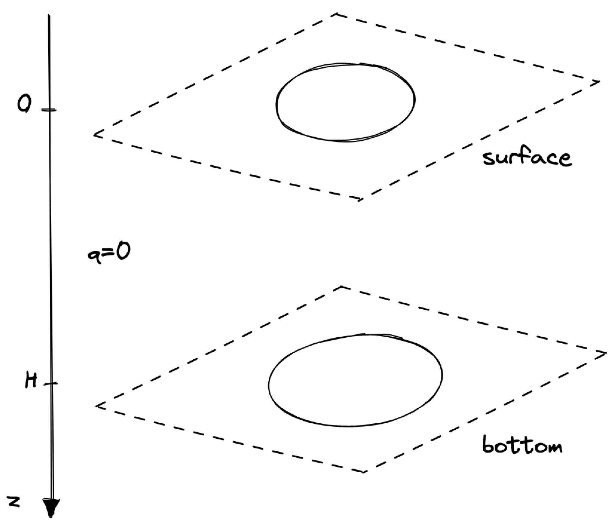
We study the instability of vortices in the Surface Quasi-Geostrophic (SQG) model. This model is discretized vertically here with two horizontal surfaces (two levels) containing a finite buoyancy for the vortices. The two horizontal surfaces are the actual surface and the bottom of the ocean (or the thermocline if the temperature—and density—gradient is sufficiently abrupt at this depth [19,20]). The two levels are vertically separated by a height H (see Figure 1). The buoyancy (or potential temperature) distributions are contained in the two levels. They are connected by a condition of zero Potential Vorticity (PV) in the interior of the domain.
The SQG model is the restriction of the complete quasi-geostrophic model—introduced by Charney in 1948 [17]—to null internal potential vorticity distributions (for more details on the SQG model, see [18,21]). Potential vorticity is thus concentrated as a vertical Dirac distribution, reducing to a planar buoyancy anomaly, at the two (upper and lower) boundaries.
Assuming constant Brunt–Vaïsala () and Coriolis () frequencies, the quasi-geostrophic model is governed by the conservation of potential vorticity q in the fluid volume, in the absence of forcing and of dissipation for the flow:
associated with the following 3D Laplace equation:
where J is the horizontal Jacobian operator and is the stream function (remember that the horizontal velocity is ). The boundary conditions of the 3D model at the top and bottom of the domain are the horizontal advection of the buoyancies b on these surfaces:
with .
The surface quasi-geostrophic equations are therefore the restriction of this model to in the fluid interior. This leads to a model defined only in terms of the surface and bottom buoyancies, related to stream function as above.
Because this work pertains to vortices, we chose the length scale L equal to the vortex radius so that our dimensionless vortex radius is here. Furthermore, we scaled the vertical coordinate z by the depth of the ocean H, so that the dimensionless ocean depth is unity also.
From this, we obtained a dimensional parameter , which is the square root of the usual Burger number. It is also equal to its dimensionless value in the model ( being scaled by and by ). The timescale T is given by our choice of unit buoyancy at the surface . By recalling that , with a vortex rotational velocity and with , and using our scaling, we obtain .
This scaling is also used at the end of our paper to compute the growth rates of the Eady baroclinic instability for oceanic vortices. Once this scaling is performed, we have the following set of equations:
where is the horizontal Lagrangian derivative and the superscripts s and b represent, respectively, “surface” and “bottom”.
The first equation of System (3) in horizontal Fourier space gives
where . This equation with Neumann boundary conditions for buoyancies gives in the Fourier space
The mean flow in our SQG model are two top-hat vortices (i.e., two vortices with constant buoyancy in a disk of radius unity). This article tackles the linear stability of this mean flow (or basic state). This problem is called the Eady baroclinic instability of this vortex. With this mean flow geometry, the polar coordinates are a natural choice.
3. Mean Flow Calculation
In this section, we calculate the flow field associated with these two top-hat vortices. Firstly, we remind about the form of cylindrical Fourier transforms.
3.1. Preliminaries about Fourier Decomposition in Cylindrical Coordinates
In cylindrical coordinates, consider a function sufficiently regular:
- representing an angle, then f is -periodic in , so can be decomposed in Fourier modes:with
- For every fixed and , the functions can be written as inverse Hankel transforms (kind of Fourier transform for radial functions):where are the Bessel functions of the first kind and with
In the end, the function can be decomposed as
with
where is the Fourier transform of f in cylindrical Fourier coordinates.
Remark 1.
For the second bullet point, the Bessel function could be arbitrary, but the n-th function is retained because it is a solution of the Laplace equation.
3.2. Application to SQG Flows
We decompose the stream function of an arbitrary flow as in (10) to obtain:
with the horizontal Fourier transform of , already computed in (5). We deduce:
Therefore, at the two boundaries (surface and bottom), we have:
Remark 2.
From now, we denote by capital letters the basic state variables and by lowercase letters the perturbed variables. For example, the total stream function at the surface will be .
3.3. Basic State: Two Top-Hat Vortices
We take as the basic state two top-hat vortices (i.e., two circular plateaus of constant buoyancy) with the same dimensionless radius , but not the same intensities and :
where is the Heaviside function.
Remark 3.
The vortices’ polarity (cyclonic or anticyclonic) is determined by the sign of , but inversely for the surface or the bottom. For example, a positive buoyancy at the surface of the ocean will tend to spread out and, so, will diverge anticyclonically, but a positive buoyancy at the bottom of the ocean will tend to converge and, so, turn cyclonically.
To have the stream function of the basic state from Equation (14), we need the Fourier transforms of the buoyancies: for , we have for because is independent of . For , because , we find . Then, the stream function for the basic state at the two boundary levels is:
The main flow at the ocean’s surface induced by the two vortices can be computed through a gradient inversion of :
The found flow is along , and we use the identity to find the angular velocity. Similarly, the flow at the bottom of the ocean is:
We now introduce the quantities:
such that the angular velocities of the basic flows at the two levels are:
Remark 4.
This is indeed a steady basic state: since there is no radial velocity, the buoyancy anomaly—which is a tracer—will remain a circular patch if unperturbed.
The graphs of and of are represented in Figure 2 for fixed . Notice that . The first inequality put in Equation (20) shows that the angular velocity at the surface (respectively bottom) is mainly induced by the buoyancy intensity at the surface (respectively bottom). The second inequality, with the sign inversion in (20), shows that, to have two vortices with different polarity, we have to choose and both positive (or both negative, but the SQG equations are parity-invariant). The graph represents the angular velocity of the mean flow at the ocean’s surface when the intensities are equal to 1 and .
4. Linear Evolution of the Vortex Boundaries under Perturbations
4.1. Framework
Now, we perturb each vortex by deforming its contour. Because , an initial plateau in buoyancy will remain such at all times (with a deformed external contour). Therefore, the lateral jump in buoyancy will always exist, and we can define the vortex boundary as the place where the jump lies. The evolution of the vortex boundaries will measure the stability of this particular basic state.
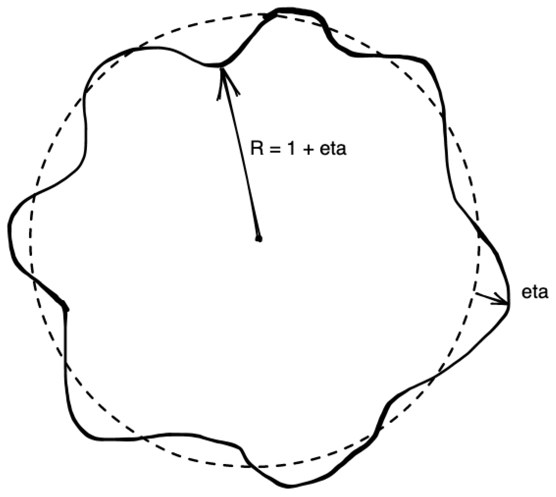
Assume that the radii and of the vortices at the surface and the bottom are disturbed from their basic states , as represented in Figure 3.
Remark 5.
We assume that, during the linear stage of instability, as the perturbation amplitude remains small, the boundary will not be locally multi-valued, such that we can use the following parameterization:
where is small compared with 1.
Then, the buoyancy at the surface is:
where H is the Heaviside function. A similar form can be derived for the buoyancy at the bottom.
4.2. Calculation of the Perturbed Quantities
Because we chose (15) as the basic buoyancies, the perturbed buoyancy (the buoyancy of the basic state minus the buoyancy of the perturbed basic state) at the surface is:
As a distribution, for small , we have . Because the derivative of H is the Dirac mass, we obtain:
where is the Dirac mass in 1.
Because the perturbed stream functions from Equation (14) are searched, we need the Fourier transforms of the perturbed buoyancies:
and a similar formula for . We find then from Equation (14) for the perturbed stream functions:
and
where and are defined in Equation (19).
4.3. Dynamics of the Perturbations
The (total and perturbed) radial flow at the boundary of the surface vortex is, on the one hand:
and on the other hand,
The justification of the first equality is the following: is the radial coordinate of a material line (the boundary of the vortex). Therefore, its rate of Lagrangian displacement in time is exactly the radial velocity of the flow.
With the equality of Equations (31) and (32), using a Taylor expansion for small amplitude perturbations (details are given in Appendix A), we obtain the following system:
where the stream functions and velocity fields are applied in .
Assuming that one mode of perturbation will grow faster than any other, we retain only one Fourier mode , so that we obtain the matrix form with :
where the integrals and , defined in Equation (19), are applied in . From now, we denote by and the previous integrals applied in , such that they depend only on .
5. Results
5.1. Preliminaries: Study of the Integrals and
We failed to compute analytically the integrals and , so from now, we perform a numerical study of the stability. Numerically, these integrals have poor convergence properties. In particular, the integral is not absolutely convergent. We present the method to compute them in Appendix B.
5.2. Normal Modes
In this section, we consider normal mode perturbations to the vortex boundaries. This means that the time dependence of is with . is called the growth rate, and is constant. In order to conclude about stability, we are now interested in the sign of , the imaginary part of . Thanks to (34), we obtain an eigenvalue problem where and
Remark 6.
As mentioned in Remark 3, if we take opposite signs for and , we will have two cyclones or anticyclones. The analysis of the stability gives a stable state whatever the mode n, the modulus of the buoyancies, or σ. Therefore, from now, we suppose and . This corresponds to the Charney–Stern criterion [22] for baroclinic instabilities.
Because is a real matrix, there are only two possibilities for the eigenvalues. They can be real, then , and the basic state has a neutral stability; or they can be complex conjugate, then one of the two eigenvalues has , and the basic state is unstable.
Remark 7.
The normal mode is always stable because
has two real eigenvalues: 0 and .
Conclusions on this flow stability were obtained by computing the discriminant of , the characteristic polynomial of :
In order to find if the roots of this polynomial are real or complex conjugate, we compute the sign of the discriminant :
The conclusion is: if , then the system is neutral because , and if , then the growth rate and the system is unstable.
Remark 8.
If we take , as Badin and Poulin in [13], we obtain , and then, we recover their dispersion relation .
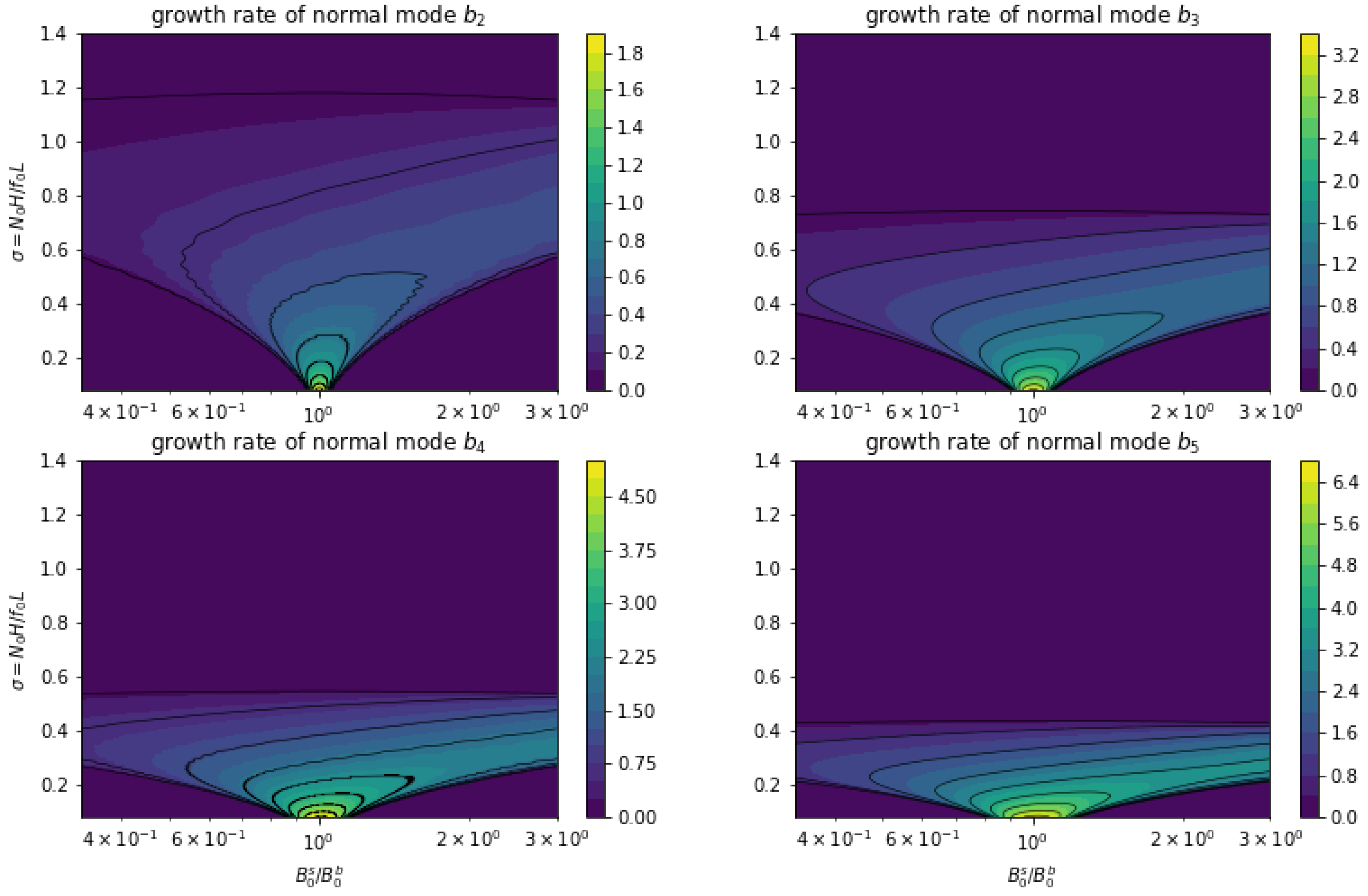
Because the case is always stable (see Remark 7), we plot in Figure 4 the normal modes for , and 5.
The dark purple zone is where . There, , and the system reaches a stable state with the following dispersion relation:
The four angular modes have similar stability properties on the top-hat vortex, but for different values of the physical parameters (). For each mode, we can separate three stable zones:
- In the upper part of each panel, where is larger than a threshold depending on n. We recover here the results of [13,14]. They found that a top-hat vortex, alone in an SQG model, is stable. In this area, the system is linearly stable for barotropic (horizontal shear) instability. They are sufficiently far from the other ( is proportional to H), so we could neglect the interactions. The two-layer SQG model is then viewed as two one-layer SQG models where there are two independent top-hat vortices. We define as the critical value of leading to instability, all other parameters being fixed. is a decreasing function with respect to n. The stability of high mode perturbations is reached for a smaller distance between vortices than low mode perturbations. This is due to the relation between horizontal and vertical wave numbers in the SQG model.
- In the bottom left and the bottom right sides of each panel, the system is also stable. In these areas, the vortices are close to each other, but have very different intensities. An interpretation of this situation could be that perturbations on one of the vortices have very different phase speeds around the contour than for the other vortex. The impossibility for these two (Rossby) waves to phase lock and resonate stabilizes the whole system.
The system is unstable if the mean buoyancy intensities are similar and if the vortices are vertically close to each other.
For a given fixed mode and a fixed ratio , an interpretation of the change of stability with is the following:
- For small , the two vortices are too close to each other for the wave to grow; thus, short-wave cut-off (usual for the Eady model) can be explained by the absence of phase locking between waves.
- For intermediate , the distance between the two vortices allows the mode to grow (phase locking with the proper phase shift is possible), and then, the system is unstable. The smaller is, the shorter the most unstable waves are.
- For large , the two vortices are far from each other, wave–wave interaction is weak, and the mode is stable.
5.3. Singular Modes
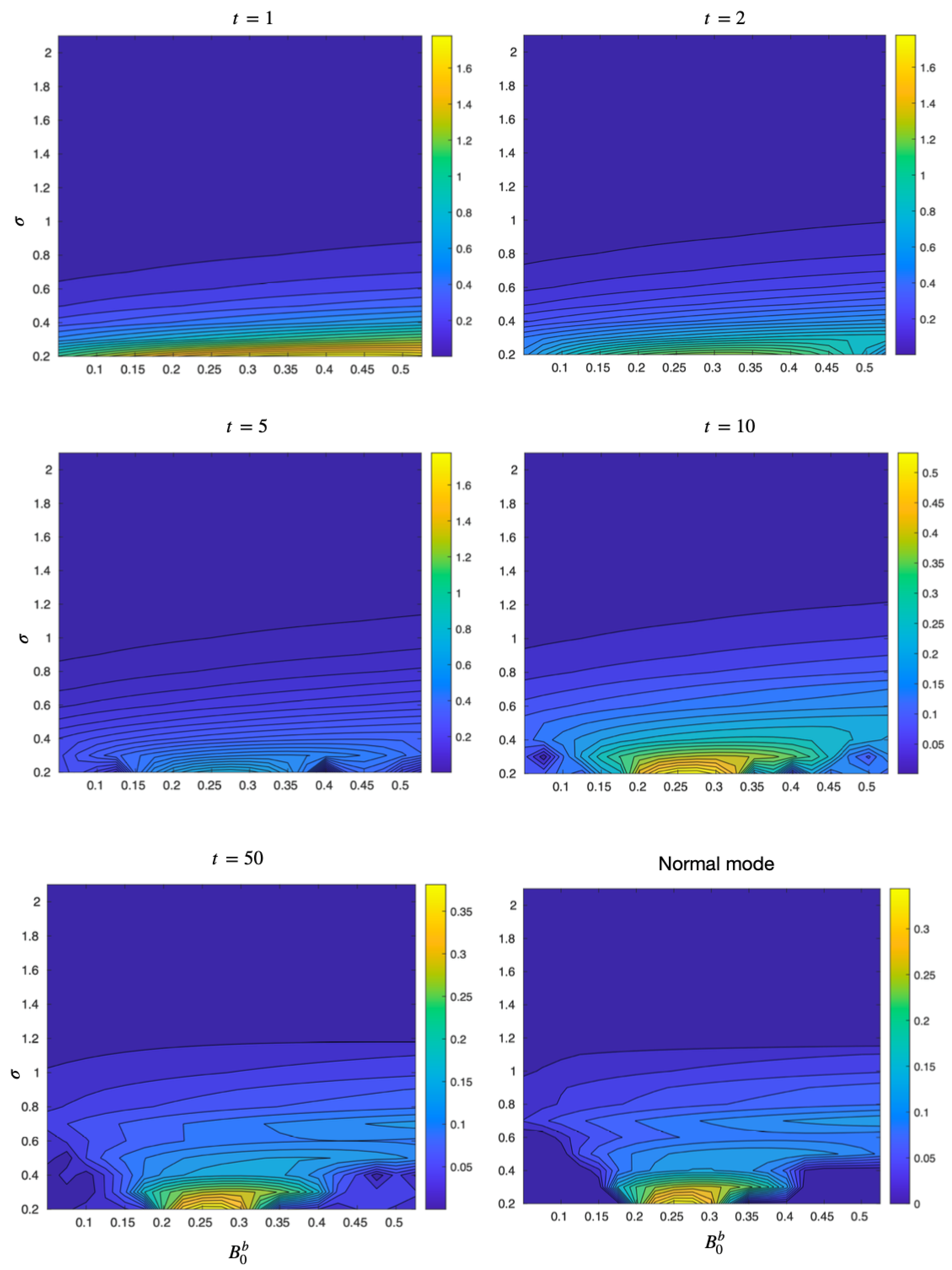
System (34) is a system, and the matrix is independent of time t. The solution is then given by . Since matrix is not self-adjoint, linear combinations of normal modes can grow faster than each normal mode considered separately [23]; they are the singular modes of the problem. Therefore, we calculate the singular modes of the stability of this vortex flow. They are defined as the maximal growth rate of a given norm of these perturbations. Here, we chose the squared perturbation buoyancy as the norm. The numerical method for singular mode calculation given in the Appendix of [24] is implemented here. The growth rates of the singular modes are the eigenvalues of the matrix . These growth rates are shown with respect to the same physical parameters () as the normal modes, for increasing values of the time t and for in Figure 5.
For small times, the singular modes’ growth rates are concentrated near the region of small . Indeed, at small times, only short waves can grow, corresponding to buoyancy surfaces close to each other vertically. Furthermore, for small , the singular mode instability occurs for every , i.e., even a weak bottom buoyancy is sufficient to allow the phase locking of these short waves. This implies that two vertically close vortices, with different mean buoyancies, are unstable for singular modes, but stable for normal modes for small times. Note that a similar remark was made in [25] about the independence of singular mode growth rates to the barotropic component of the flow at small times. As time grows, the singular mode growth rates for converge towards those of the corresponding normal modes; this result is valid for the other . This confirms the result of previous studies [23,24,25].
6. Conclusions and Perspectives
In this study, we developed analytically and numerically the calculation of the growth rates for the instability of two superposed vortices. The theory and the computation of the mean flow were first performed analytically. The computation of the normal and singular modes was performed numerically. The two-level SQG model and the considered steady state were idealized, but they provide simple results for the Eady baroclinic instability of two superposed vortices: stability for vertically distant vortices; instability for vertically close vortices similar in intensity; and instability in singular modes only for small times for vertically close vortices, even with different intensities.
Though these results pertain to idealized vortices, we can apply them to the ocean. Using the following values s, s, m, m, m/s, where V is the rotational velocity of an oceanic vortex, we obtained the following length and time scales, m, s. Firstly, we can use the values of to determine which vortices can be unstable: strong instability occurs for leading to most unstable vortices having a thickness of 100 m, which indeed corresponds to small vortices (with radii close to 10 km). Secondly, we can compute the growth rates of such normal mode perturbations in the ocean: in dimensionless terms, they are on the order of for . This corresponds to a typical time scale for the growth of these perturbations of s, which is about days. This timescale is slightly shorter than that found in the two-layer Phillips problem of mesoscale vortex baroclinic instability, which is about 4 days [6,25].
Finally, we must also note that we studied only the linear instability of such vortices. The natural follow-up of these calculations is the study of the long-term, nonlinear evolution of these unstable vortices. This will indicate if the linearly unstable waves found here can be stabilized in the long run via nonlinear wave interactions and the shape the nonlinearly stabilized vortices would take. Furthermore, this will allow the variation of several parameters not included here:
- Investigate the effect of different radii for the two vortices;
- Shift one vortex with respect to the other and study the evolution of tilted vortices;
- Consider two different modes and of perturbation for the two vortices;
- Consider other radial shapes for the vortices (Gaussian, etc.).
This numerical study is under way and will complement this first paper.
Author Contributions
Conceptualization, X.C. and J.G.; methodology, X.C. and A.V.; validation, A.V., X.C. and J.G.; formal analysis, A.V. and X.C.; writing—original draft preparation, A.V.; writing—review and editing, A.V. and X.C.; supervision, X.C. and J.G. All authors have read and agreed to the published version of the manuscript.
Funding
This research was supported by external funding: the first author received a Ph.D. grant from École Normale Superieure, Rennes. This work is also a contribution to the EUREC4A-OA oceanographic program.
Acknowledgments
This work is a contribution to the JPI Ocean and Climate project EUREC4A-OA, with additional support from CNES (the French National Centre for Space Studies).
Conflicts of Interest
The authors declare no conflict of interest. The funders had no role in the design of the study; in the collection, analyses, or interpretation of the data; in the writing of the manuscript; nor in the decision to publish the results.
Appendix A. Proof of the System Descibing the Dynamics of the Perturbations
We develop the calculus for the surface only. The bottom case is similar. If we consider that all the perturbed quantities , , and all their derivatives are of order , we have, on the one hand, from Equation (31):
On the other hand, from Equation (32), we have:
Then, at the order , we obtain
Remark A1.
Note a difficulty we did not mention earlier: is not differentiable in the classical way. Formally, we should work with a smooth approximation of top-hat vortices and then move on to the limit.
Appendix B. Proof of Convergence and Numerical Method to Compute In − I1 and Mn
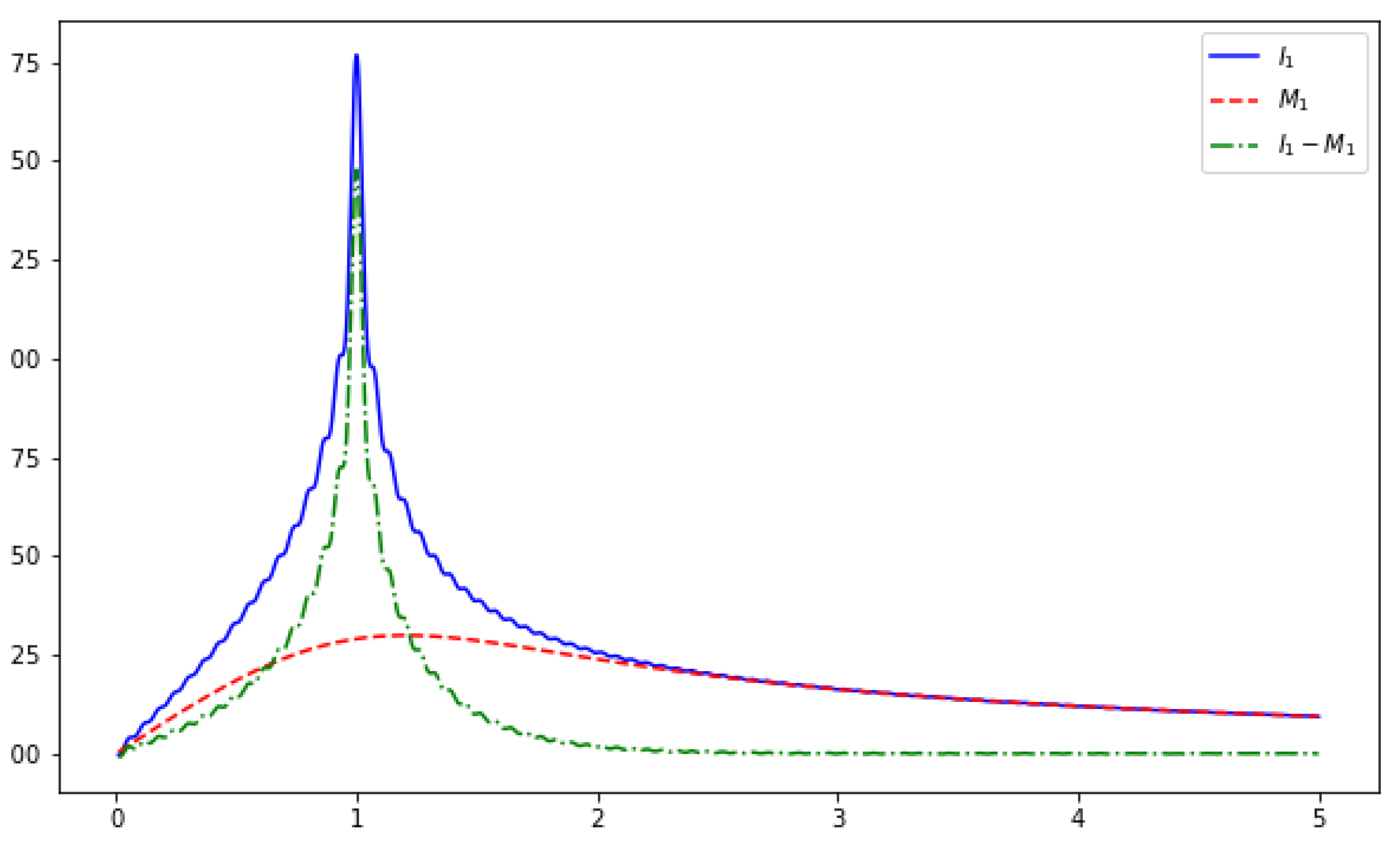
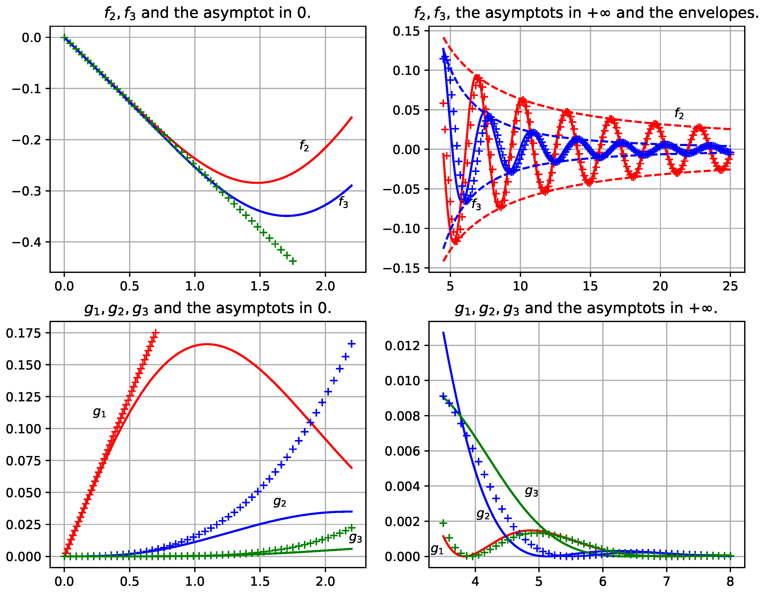
Recall and with and (see Figure A1). The two functions are continuous on . Let us perform the analysis of convergence in 0 and in ∞. All the approximations used here were derived previously by the scientific community and are not proven again:
- For x in a neighborhood of 0, so for :and for :Therefore, the two functions are integrable in 0.
- For x in a neighborhood of ,The computation gives for :and for :We can quickly conclude for the odd case because is absolutely convergent in . The even case is a modified integral sine, so that it converges.For every , we have a quick convergence in for :
Figure A1.
The integrands and are in the solid line; the asymptotes are plotted with crosses; the envelops for the top right panel are in dashed lines. Notice that for the bottom right panel, the asymptote depends only on the parity of n. This explains why there are only two asymptotes plotted. Here, we take the parameter .

Numerically, the only difficult point is the fact that the integral sine does not absolutely converge, so that the classically implemented methods to compute integrals are not adapted. A python routine exists to compute the integral sine, and this is what we used. The idea is to cut the integrals into three parts, , to use approximation for the integrals in 0 and in , and to use the classical python routine in . With the asymptotic developments we used, we obtain:
- For in 0:
- For in :where is the integral sine function.
- For in :
- For in 0:
- For in :Therefore, if we take sufficiently large (in practice, we take ), this part can be neglected.
The following Table A1 sums up the approximations we used to compute the integrals and .

Table A1.
Summary of the approximated integrals.
| 0 |
Appendix C. Nomenclature
| q | Potential Vorticity (PV) |
| J | Jacobian operator |
| H | the distance between the two vortices or the Heaviside function |
| L | the horizontal scale of the dynamics |
| stream function of the total or perturbed flow (from Remark 2) | |
| b | buoyancy |
| Brunt–Vaïsala frequency | |
| Coriolis frequency | |
| the radii of the vortices | |
| horizontal Lagrangian derivative: | |
| square root of the Burger number | |
| intensities of the two steady vortices | |
| K | horizontal Fourier variable |
| radial, angular, and vertical coordinates in the cylindrical system | |
| Bessel functions of the first kind | |
| Fourier transform of any function f | |
| total or perturbed stream functions at the two levels | |
| stream functions of the basic state at the two levels | |
| buoyancies of the basic state at the two levels | |
| intensities of the buoyancies of the basic state | |
| radial velocities of the basic state at the two levels | |
| angular velocities of the basic state at the two levels | |
| integrals defined in Equation (19); from Equation (34), applied in | |
| perturbation of the vortices’ radii | |
| the Dirac mass in 1 | |
| multiplicative constants of the normal modes | |
| the normal mode of the perturbation | |
| matrix defined in Equation (35) | |
| characteristic polynomial of : | |
| discriminant of the second-order polynomial | |
| and | respectively, integrands of and |
| size of the perturbation | |
| Landau notation; design any function bounded by when | |
| f is similar to g in if and | |
| factorial n: | |
| Si | is the integral sine function |
References
- Provenzale, A. Transport by Coherent Barotropic Vortices. Annu. Rev. Fluid Mech. 1999, 31, 55–93. [Google Scholar] [CrossRef] [Green Version]
- Fratantoni, D.M.; Richardson, P.L. The Evolution and Demise of North Brazil Current Rings. J. Phys. Oceanogr. 2006, 36, 1241–1264. [Google Scholar] [CrossRef] [Green Version]
- Richardson, P.L.; Bower, A.S.; Zenk, W. A census of meddies tracked by floats. Prog. Oceanogr. 2000, 45, 209–250. [Google Scholar] [CrossRef]
- Laxenaire, R.; Speich, S.; Blanke, B.; Chaigneau, A.; Pegliasco, C.; Stegner, A. Anticyclonic eddies connecting the western boundaries of Indian and Atlantic Oceans. J. Geophys. Res. Ocean. 2018, 123, 7651–7677. [Google Scholar] [CrossRef]
- De Marez, C.; Meunier, T.; Morvan, M.; L’Hegaret, P.; Carton, X. Study of the stability of a large realistic cyclonic eddy. Ocean. Model. 2020, 146, 101540. [Google Scholar] [CrossRef]
- Flierl, G.R. On the instability of geostrophic vortices. J. Fluid Mech. 1988, 197, 349–388. [Google Scholar] [CrossRef]
- Carton, X.J.; McWilliams, J.C. Nonlinear oscillatory evolution of a baroclinically unstable geostrophic vortex. Dyn. Atmos. Ocean. 1996, 24, 207–214. [Google Scholar] [CrossRef]
- Baey, J.M.; Carton, X. Vortex multipoles in two-layer rotating shallow-water flows. J. Fluid Mech. 2002, 460, 151–175. [Google Scholar] [CrossRef] [Green Version]
- Carton, X. Instability of Surface Quasigeostrophic Vortices. J. Atmos. Sci. 2009, 66, 1051–1062. [Google Scholar] [CrossRef]
- Menesguen, C.; Le Gentil, S.; Marchesiello, P.; Ducousso, N. Destabilization of an Oceanic Meddy-Like Vortex: Energy Transfers and Significance of Numerical Settings. J. Phys. Oceanogr. 2018, 48, 1151–1168. [Google Scholar] [CrossRef]
- McDougall, T.J. Double-diffusive interleaving. Part 1. J. Phys. Oceanogr. 1985, 15, 1532–1541. [Google Scholar] [CrossRef] [Green Version]
- Shapiro, G.I. On the Dynamics of Lens-like Eddies. Elsevier Oceanogr. Ser. 1989, 50, 383–396. [Google Scholar]
- Badin, G.; Poulin, F.J. Asymptotic scale-dependent stability of surface quasi-geostrophic vortices: Semi-analytic results. Geophys. Astrophys. Fluid Dyn. 2019, 113, 574–593. [Google Scholar] [CrossRef]
- Harvey, B.J.; Ambaum, M.H.P. Perturbed Rankine vortices in surface quasi-geostrophic dynamics. Geophys. Astrophys. Fluid Dyn. 2011, 105, 377–391. [Google Scholar] [CrossRef]
- Lapeyre, G.; Klein, P. Dynamics of the Upper Oceanic Layers in Terms of Surface Quasigeostrophy Theory. J. Phys. Oceanogr. 2006, 36, 165–176. [Google Scholar] [CrossRef]
- Klein, P.; Hua, B.L.; Lapeyre, G.; Capet, X.; Le Gentil, S.; Sasaki, H. Upper Ocean Turbulence from High-Resolution 3D Simulations. J. Phys. Oceanogr. 2008, 38, 1748–1763. [Google Scholar] [CrossRef] [Green Version]
- Charney, J.G. On the Scale of Atmospheric Motions; Geofys. Publikasjoner: Oslo, Norway, 1948; pp. 1–17. [Google Scholar]
- Lapeyre, G. Surface Quasi-Geostrophy. Fluids 2017, 2, 7. [Google Scholar] [CrossRef]
- Tulloch, R.; Smith, K.S. Quasigeostrophic Turbulence with Explicit Surface Dynamics: Application to the Atmospheric Energy Spectrum. J. Atmos. Sci. 2009, 66, 450–467. [Google Scholar] [CrossRef]
- Smith, K.S.; Bernard, E. Geostrophic turbulence near rapid changes in stratification. Phys. Fluids 2013, 25, 046601. [Google Scholar] [CrossRef] [Green Version]
- Held, I.; PierreHumbert, R.T.; Garner, S.T.; Swanson, K.L. Surface quasi-geostrophic dynamics. J. Fluid Mech. 1995, 282, 1–20. [Google Scholar] [CrossRef]
- Charney, J.G.; Stern, M.E. On the Stability of Internal Baroclinic Jets in a Rotating Atmosphere. J. Atmos. Sci. 1962, 19, 159–172. [Google Scholar] [CrossRef] [Green Version]
- Rivière, G.; Hua, B.L.; Klein, P. Influence of the beta-effect on non-modal baroclinic instability. Q. J. R. Meteorol. Soc. 2001, 127, 1375–1388. [Google Scholar]
- Fischer, C. Linear Amplification and Error Growth in the 2D Eady Problem with Uniform Potential Vorticity. J. Atmos. Sci. 1998, 55, 3363–3380. [Google Scholar] [CrossRef]
- Carton, X.; Flierl, G.R.; Perrot, X.; Meunier, T.; Sokolovskiy, M. Explosive instability of geostrophic vortices. Part 1. Baroclinic instability. Theor. Comput. Fluid Dyn. 2010, 24, 125–130. [Google Scholar] [CrossRef] [Green Version]
Figure 1.
Scheme of the two horizontal layers.

Figure 2.
Graphs of , , and as functions of r, for constant.

Figure 3.
Perturbation of the buoyancy disk, with .

Figure 4.
for , and 5, with respect to and . Be aware that the color bar differs for each panel.

Figure 5.
Singular mode for for different times . Here, . The bottom right panel represents the growth rates for normal mode . We can note the convergence of singular modes to normal modes.
Figure 5.
Singular mode for for different times . Here, . The bottom right panel represents the growth rates for normal mode . We can note the convergence of singular modes to normal modes.

Publisher’s Note: MDPI stays neutral with regard to jurisdictional claims in published maps and institutional affiliations. |
© 2022 by the authors. Licensee MDPI, Basel, Switzerland. This article is an open access article distributed under the terms and conditions of the Creative Commons Attribution (CC BY) license (https://creativecommons.org/licenses/by/4.0/).
Share and Cite
MDPI and ACS Style
Vic, A.; Carton, X.; Gula, J. Eady Baroclinic Instability of a Circular Vortex. Symmetry 2022, 14, 1438. https://doi.org/10.3390/sym14071438
AMA Style
Vic A, Carton X, Gula J. Eady Baroclinic Instability of a Circular Vortex. Symmetry. 2022; 14(7):1438. https://doi.org/10.3390/sym14071438
Chicago/Turabian StyleVic, Armand, Xavier Carton, and Jonathan Gula. 2022. "Eady Baroclinic Instability of a Circular Vortex" Symmetry 14, no. 7: 1438. https://doi.org/10.3390/sym14071438
Note that from the first issue of 2016, this journal uses article numbers instead of page numbers. See further details here.