
MTV-MFO: Multi-Trial Vector-Based Moth-Flame Optimization Algorithm
by
 , , , and
Mohammad H. Nadimi-Shahraki
1,2,* ,
,
Shokooh Taghian
1,2 ,
,
Seyedali Mirjalili
3,4,* ,
,
Ahmed A. Ewees
5,
Laith Abualigah
6,7 and
and
Mohamed Abd Elaziz
8,9,10,11
1
Faculty of Computer Engineering, Najafabad Branch, Islamic Azad University, Najafabad 1584743311, Iran
2
Big Data Research Center, Najafabad Branch, Islamic Azad University, Najafabad 1584743311, Iran
3
Centre for Artificial Intelligence Research and Optimisation, Torrens University Australia, Fortitude Valley, QLD 4006, Australia
4
Yonsei Frontier Lab, Yonsei University, Seodaemun-gu, Seoul 03722, Korea
5
Department of Computer, Damietta University, Damietta 34511, Egypt
6
Faculty of Computer Sciences and Informatics, Amman Arab University, Amman 11953, Jordan
7
School of Computer Sciences, Universiti Sains Malaysia, Pulau Pinang 11800, Malaysia
8
Department of Mathematics, Faculty of Science, Zagazig University, Zagazig 44519, Egypt
9
Artificial Intelligence Research Center (AIRC), Ajman University, Ajman 346, United Arab Emirates
10
Department of Artificial Intelligence Science & Engineering, Galala University, Suze 435611, Egypt
11
School of Computer Science and Robotics, Tomsk Polytechnic University, 634050 Tomsk, Russia
*
Authors to whom correspondence should be addressed.
Symmetry 2021, 13(12), 2388; https://doi.org/10.3390/sym13122388
Submission received: 13 November 2021
/
Revised: 3 December 2021
/
Accepted: 6 December 2021
/
Published: 10 December 2021
(This article belongs to the Special Issue Meta-Heuristics for Manufacturing Systems Optimization)
Abstract
:The moth-flame optimization (MFO) algorithm is an effective nature-inspired algorithm based on the chemical effect of light on moths as an animal with bilateral symmetry. Although it is widely used to solve different optimization problems, its movement strategy affects the convergence and the balance between exploration and exploitation when dealing with complex problems. Since movement strategies significantly affect the performance of algorithms, the use of multi-search strategies can enhance their ability and effectiveness to solve different optimization problems. In this paper, we propose a multi-trial vector-based moth-flame optimization (MTV-MFO) algorithm. In the proposed algorithm, the MFO movement strategy is substituted by the multi-trial vector (MTV) approach to use a combination of different movement strategies, each of which is adjusted to accomplish a particular behavior. The proposed MTV-MFO algorithm uses three different search strategies to enhance the global search ability, maintain the balance between exploration and exploitation, and prevent the original MFO’s premature convergence during the optimization process. Furthermore, the MTV-MFO algorithm uses the knowledge of inferior moths preserved in two archives to prevent premature convergence and avoid local optima. The performance of the MTV-MFO algorithm was evaluated using 29 benchmark problems taken from the CEC 2018 competition on real parameter optimization. The gained results were compared with eight metaheuristic algorithms. The comparison of results shows that the MTV-MFO algorithm is able to provide competitive and superior results to the compared algorithms in terms of accuracy and convergence rate. Moreover, a statistical analysis of the MTV-MFO algorithm and other compared algorithms was conducted, and the effectiveness of our proposed algorithm was also demonstrated experimentally.
1. Introduction
Metaheuristic algorithms have been shown to be effective due to complex characteristics of difficult optimization problems such as dimensionality, multimodality, and non-differentiability [1]. Due to the growing complexity of optimization problems and compared to conventional optimization algorithms, metaheuristics have proven their ability to solve complex problems by providing feasible solutions in a reasonable time [2]. Thus, there is an increasing trend to propose new algorithms and enhance the performance of existing algorithms using improvement strategies [3]. Among the metaheuristics, nature-inspired algorithms that draw inspiration from natural phenomena to create new and more resilient competitive algorithms are prominent. Several new optimization algorithms have been proposed recently due to the No-free-lunch (NFL) theorem [4], which states that no particular optimization algorithm can solve all problems of all kinds of complexities. It is also observed that depending on the set of parameter values, the same algorithm produces different solutions to the same problem.
Metaheuristic algorithms simulate intelligent behavior from different aspects of creatures in nature to derive rules for optimization purposes. In population-based metaheuristic algorithms, a population of individuals is distributed over a boundary-limited search space in which they try to move toward the best solution by exchanging information. Some well-known and recently proposed metaheuristic algorithms in this regard are the particle swarm optimization algorithm (PSO) [5], genetic algorithm (GA) [6], whale optimization algorithm (WOA) [7], polar bear optimization (PBO) algorithm [8], salp swarm algorithm (SSA) [9], red fox optimization (RFO) algorithm [10], and quantum-based avian navigation optimizer algorithm (QANA) [11]. The salient features of metaheuristic algorithms such as flexibility, derivation-free nature, and simplicity in implementation allow them to be utilized in a wide range of problems in different fields including, but not limited to, classification [12], healthcare [13], engineering [14,15], power and energy management [16], data analysis [17], and image segmentation [18].
Population-based optimization algorithms have some common drawbacks, such as lack of exploration or exploitation ability, inappropriate balance between exploration and exploitation, slow or premature convergence behavior, and stagnation in local optima [19]. In this regard, new strategies have been integrated into existing algorithms to design an effective algorithm that can handle these defects. Some of these successful improvements use strategies including opposition-based learning [20,21], levy flight [22,23], mutation [24,25], rough sets [26,27], and chaotic maps [28,29].
The moth-flame optimization (MFO) [30] algorithm is one of the nature-inspired algorithms that simulates the behavior of moths to navigate in nature. Moths fly at a constant angle with the moon, called transverse orientation, which is an effective mechanism for moving in a straight line over long distances. However, in the face of artificial lights, the use of transverse orientation causes a spiral path to the light source. In this population-based algorithm, the population of moths is directed by considering the distance to the corresponding flame. Although the concept of MFO is simple, it has the potential to be one of the flagship optimization algorithms, and accordingly, many improvements and applications of MFO have been proposed. The MFO algorithm has been used in various applications such as engineering problems [31], feature selection [32], medical diagnosis [29], global optimization [24], price forecasting [33], photovoltaic energy generation systems [34], power correction [35], wind speed distribution [36], and economic load dispatch problems [37].
Despite the fact that MFO has been employed to tackle a variety of issues, it still has flaws such as premature convergence and insufficiently balanced exploitation and exploration [38,39]. These shortcomings originate from the MFO movement strategy, which has a single guiding strategy that causes ineffective performance when dealing with different kinds of problems. Therefore, equipping the MFO algorithm with multi-movement strategies can enhance its ability and effectiveness. We proposed a multi-trial vector (MTV) approach in our previous study [40] to combine complementary movement strategies with simple metaheuristic algorithms such as MFO so that their frameworks can be adapted to the MTV approach. Improving the MFO algorithm using a sufficient combination of movement strategies and adapting them to the MFO’s movement strategy through the MTV approach to solve different complex optimization problems such as shifted or shifted rotated problems was our main motivation for this study.
In this paper, we propose a multi-trial vector-based moth-flame optimization (MTV-MFO) algorithm using the multi-trial vector approach. The MTV approach replaces the spiral movement strategy of the MFO to obtain better performance when dealing with various optimization problems. By embedding the MTV approach in the MFO algorithm, different kinds of trial vector producers (TVPs) can be defined, each of which is suitable to sustain a specific behavior during the optimization process. In addition, each defined TVP can be applied to a dedicated portion of the population by using the MTV’s winner-based distribution policy. In the MTV-MFO algorithm, two new proposed movement strategies—the flag-guided trial vector producer (F-TVP) and contingent trial vector producer (C-TVP)—are incorporated with the canonical moth-flame trial vector producer (MFO-TVP). Furthermore, MTV-MFO employs inferior moth information preserved in two external archives to prevent trapping in local optima and premature convergence. The combination of three TVPs and the use of archives in the proposed MTV-MFO enrich the balance between exploration and exploitation, reduce the local optima trapping, and prevent premature convergence. To validate the proposed MTV-MFO algorithm, experiments were performed on 29 test functions derived from the special session on real-parameter optimization of CEC 2018 [41]. The results were compared with state-of-the-art nature-inspired metaheuristic algorithms including the krill herd (KH) [42], grey wolf optimizer (GWO) [43], moth-flame optimization (MFO) [30], whale optimization algorithm (WOA) [7], salp swarm algorithm (SSA) [9], butterfly optimization algorithm (BOA) [44], henry gas solubility optimization (HGSO) [45], and Archimedes optimization algorithm (AOA) [46]. Moreover, the proposed algorithm was statistically analyzed by the Friedman test and student’s t-test. Additionally, the box plot analysis was performed to check the consistency of the proposed algorithm. Based on the comparison of results, the MTV-MFO demonstrated superiority on most test problems.
Briefly, the contributions of this paper can be summarized as follows.
- The canonical MFO is modified by substituting the transverse orientation of MFO with the MTV approach to enhance the performance of the original MFO.
- In the flag-guided trial vector producer (F-TVP), the flag flame is introduced with the aim of enhancing the exploration ability of the original MFO. Besides that, the best flame is employed to calculate the distance between moth and flames. Additionally, a new spiral function is used to model the flying path of moths.
- In the contingent trial vector producer (C-TVP), two new external archives are employed to increase exploratory capability and diversity. Additionally, the position of the best moth is considered as the base vector to change the moths’ positions with respect to the current best moth position.
- The proposed MTV-MFO algorithm concurrently executes three trial vector producers on the dedicated portion of the population based on the TVP’s improved rate. Experimental results demonstrate that the MTV-MFO performs better than the canonical MFO and other state-of-the-art nature-inspired algorithms.
The rest of the paper is organized as follows. In Section 2, the related works are reviewed. Section 3 presents the mathematical model and flowchart of the MFO algorithm. Section 4 contains the proposed MTV-MFO algorithm. The experimental evaluation of the MTV-MFO and comparative algorithms is presented in Section 5, and the statistical analysis in Section 6. Finally, the conclusions and future works are given in Section 7.
2. Related Work
Metaheuristic algorithms, especially nature-inspired ones, have proven their superiority in solving complex optimization problems compared to deterministic algorithms [47]. Nature-inspired metaheuristic algorithms based on inspiration are mainly divided into three categories: evolutionary, swarm intelligence, and physics-based algorithms. The principles of natural evolutionary behavior are mimicked by evolutionary algorithms. Differential evolution (DE) [48], evolution strategy (ES) [49], genetic algorithm (GA) [6], and evolutionary programming (EP) [50] are some prominent algorithms in this category. The social behavior of swarms in nature is the inspiration for swarm intelligence algorithms. Particle swarm optimization (PSO) [5], artificial bee colony (ABC) [51], social spider optimization (SSO) [52], and Aquila optimizer (AO) [53] are some of the most popular or newly proposed algorithms in this area. Proposed physics-based algorithms use the fundamental physical concepts that exist in nature. Simulated annealing (SA) [54], central force optimization (CFO) [55], atom search optimization (ASO) [56], and the Lichtenberg algorithm (LA) [57] are some well-known or recently proposed algorithms in this category.
The emergence of optimization problems with diverse characteristics in different fields leads to a trend toward effective algorithms that are able to find appropriate solutions. Therefore, it is still necessary to propose new algorithms or improve existing algorithms to eliminate their defects. These algorithms have been used to solve several real-world problems in both continuous and discrete spaces such as feature selection [58,59,60,61], scheduling and planning [62], disease diagnosis [63], engineering problems [64], photovoltaic energy generation systems [65,66], economic dispatch problems [67], global optimization [68,69,70], community detection [71,72,73], and motion estimation [74,75]. Among swarm intelligence algorithms, the moth flame optimization (MFO) algorithm has attracted noticeable interest for optimization purposes. MFO is applied in various fields, including training multi-layer perceptrons [76], optimal reactive power dispatch [77], terrorism prediction [78], optical network unit placement [79], optimal sizing of an isolated micro-grid [80], and dynamic performance enhancement for wind energy conversion systems [81].
In general, the metaheuristic algorithms have two common behaviors: exploration (diversification) and exploitation (intensification). Exploration refers to the algorithm’s ability to search the entire search space to find new solutions by scattering random individuals and moving through the search space to investigate different regions of the search space. Exploitation refers to the ability of the algorithm to find the optimum solution near a previously discovered solution. An effective optimization algorithm must sustain the balance of exploration and exploitation to avoid being trapped at the local optimum. Moreover, the lack of either stage leads to premature or slow convergence, stagnation, and lost diversity. The concept of simultaneously employing multiple search/movement strategies has been studied in earlier optimization techniques and has been beneficial to achieve better performance in many types of problems. Thus, using different strategies in the whole search process guarantees diversity, exploration, exploitation, and balance between them. It also increases the chance of finding the best solution to a complex optimization problem with a large search space.
In the literature, several algorithms have been proposed that use multiple strategies and operations to increase exploration and exploitation abilities, such as MEPSO [82], MAPSO [83], MSODPSO [84], HCLDMS-PSO [85], EABC [86], MEGWO [87], I-GWO [88], ESSA [89], SaDE [90], CoDE [91], AMPDE [92], and MTDE [40]. In [82], multi-strategy ensemble particle swarm optimization (MEPSO) was proposed, in which the particles of the population were divided into two parts, I and II. The Gaussian local search and differential mutation incorporated the conventional PSO search strategy to guide the search process. Analysis showed that the strategy used in part I can enhance the convergence of the algorithm while the other strategy can extend the exploration ability and local optima avoidance. In [83], a multi-strategy adaptive particle swarm optimization (MAPSO) was proposed to search the global optimum in the entire search space with a very fast convergence speed. MAPSO developed an innovative strategy of diversity measurement to evaluate the population distribution and performed a real-time alternating strategy to determine one of two predefined evolutionary states at each iteration.
In [84], the authors developed the multiple strategies-based orthogonal design PSO (MSODPSO), in which a pool of auxiliary vector generation strategies is used. The social-only model or the cognition-only model was utilized in each particle’s velocity update, and an orthogonal design (OD) method was used with a small probability to construct a new exemplar in each iteration. In [85], the authors present a heterogeneous comprehensive learning and dynamic multi-swarm particle swarm optimizer (HCLDMS-PSO) using two mutation operators. The main population is divided into two sub-populations, exploitation and exploitation exemplar, employing each strategy. In [86], an enhanced artificial bee colony (EABC) algorithm was proposed to improve ABC’s performance. In the proposed EABC algorithm, two new search equations are used to generate candidate solutions for the employed bee and the onlooker bee steps. This improvement helps to balance the exploration and exploitation and improve searchability. The experimental results with a set of benchmark functions proved the proposed algorithm outperformed the canonical ABC in terms of convergence speed and quality of obtained solution.
An enhanced version of grey wolf optimizer, namely multi-strategy ensemble grey wolf optimizer (MEGWO) [87], was designed to solve the feature selection problem in real-world applications. The authors proposed the enhanced global best lead strategy, adaptable cooperative strategy, and dispersed foraging strategy to boost the performance of GWO. In MEGWO, three sets of search approaches integrate to update the wolves’ positions. Simulation results show that their proposed technique performed better than other algorithms compared. In [88], an improved grey wolf optimizer (I-GWO) was proposed to improve the search strategy of the conventional GWO algorithm. In this improvement, a new dimension learning-based hunting search strategy was proposed to tackle imbalanced exploration and exploitation and premature convergence weaknesses. In [89], a multi-strategy enhanced salp swarm algorithm (ESSA) was proposed for global optimization. In ESSA, several strategies were used to improve SSA performance, including opposition-based learning, orthogonal learning, and quadratic interpolation. The results obtained with benchmark functions demonstrated its superiority in achieving better results and convergence.
In [90], the differential evolution algorithm with strategy adaptation (SaDE) was proposed to simultaneously implement two mutation strategies in which the control parameters F and CR are self-adapted based on prior experience. In [91], the authors proposed a composite DE (CoDE) that used three strategies with three control parameter settings. To generate new trial vectors for each individual, a search strategy and parameters are selected at random. An adaptive multi-population differential evolution (AMPDE) algorithm for continuous multi-objective optimization, in which the sub-populations’ size was adaptively adjusted depending on the information gained from the previous search knowledge, was developed in [92]. To generate perturbed vectors, individuals of each sub-population changed according to the allocated crossover operator taken from GAs. In recent work, a practical approach named multi-trial vector (MTV) that can handle multiple strategies by defining and controlling the policies, dividing the population into multiple sub-populations, and using different archives was proposed in [40]. This approach can be applied to algorithms from each category. Based on this approach an effective multi-trial vector-based differential evolution (MTDE) algorithm was proposed in which three trial vector producers were defined, each of which is applied to a group of individuals. Moreover, a life-time archive is used to archive inferior solutions that help to exchange information and maintain diversity.
3. Moth Flame Optimization (MFO) Algorithm
The moth-flame optimization (MFO) [30] algorithm is a simple swarm intelligence algorithm based on the chemical effect of light on moths as an animal with bilateral symmetry [93]. The MFO algorithm simulates the navigation of moths in nature, called transverse orientation, in which moths keep a constant angle at a distance to the moon when flying at night. This orientation is an effective mechanism for moving in a straight line over long distances. However, in the face of artificial lights, the use of transverse orientation causes a spiral path to the light source. Similarly, to other population-based metaheuristic algorithms, MFO starts by randomly distributing N number of moths in a D-dimensional search space. In each iteration, the population of moths is directed by considering the distance to the corresponding flame. Then, the moths’ fitness is calculated to determine the best positions of the moths, and the optimal positions are considered as flames. Based on the inspiration, the MFO uses a logarithmic spiral in Equation (1) to update the moths’ positions around the search space.
where Di indicates the distance between the ith moth and jth flame that is calculated by Equation (2), b is a constant value equal to 1 to shape the logarithmic spiral of the movement, and t is a random number in [–1, 1].
The spiral movement in MFO depicts the flying moths’ spiral paths, which update their positions with respect to the positions of the flames. The distance between a moth and its corresponding flame is determined by the parameter t, in which t = −1 indicates the closest proximity to the flame and t = 1 represents the furthest proximity to the flame in all directions in the search space. The number of flames decreases through progressive iterations by Equation (3),
where N is the total number of moths, l indicates the current iteration, and T is the maximum number of iterations.
4. Multi-Trial Vector-Based Moth-Flame Optimization (MTV-MFO) Algorithm
Although the MFO algorithm is easy to implement and applicable to solve various optimization problems, such as optimal power flow, scheduling problems, and traveling salesman, the effectiveness of the algorithm in dealing with different complex problems is still unsatisfying. Generally, the success of algorithms in solving problems with diverse characteristics such as uni-modality or multi-modality with flat or rigid search space depends on the choices of the movement strategies and parameters. Consequently, based on the NFL theorem, there is no single movement strategy in an algorithm that can outperform other strategies and cope with diverse optimization problems. This implies that it would be beneficial to use different movement strategies in an algorithm to solve problems with diverse characteristics, such as multimodality, non-separability, and dimensionality. Motivated by these considerations, the multi-trial vector-based moth-flame optimization (MTV-MFO) algorithm is proposed to tackle the MFO algorithm’s flaws while attempting to preserve its simplicity. The premature convergence to local optima and insufficient balance between exploration and exploitation are the MFO algorithm’s weaknesses. As a result of these flaws, the MFO algorithm fails to solve a variety of complex problems.
In this paper, the MTV approach replaces the single spiral movement strategy of the MFO algorithm to obtain better performance when dealing with various and complex optimization problems. By embedding the MTV approach in the MFO algorithm, different types of trial vector producers (TVPs) can be defined, each of which is suitable to sustain a specific behavior during the optimization process. In addition, each defined TVP can be applied to a dedicated portion of the population using the MTV’s winner-based distribution policy. Hence, the exchange of information between moths from different sub-populations during population distribution can improve the MTV-MFO algorithm’s optimization efficiency. In the proposed MTV-MFO algorithm, two new movement strategies, flag-guided trial vector producer (F-TVP) and contingent trial vector producer (C-TVP), are incorporated with the original spiral movement of the MFO to reduce the local optima trapping, prevent premature convergence, and enrich the balance between exploration and exploitation. In the following, the proposed MTV-MFO algorithm’s steps are described in detail.
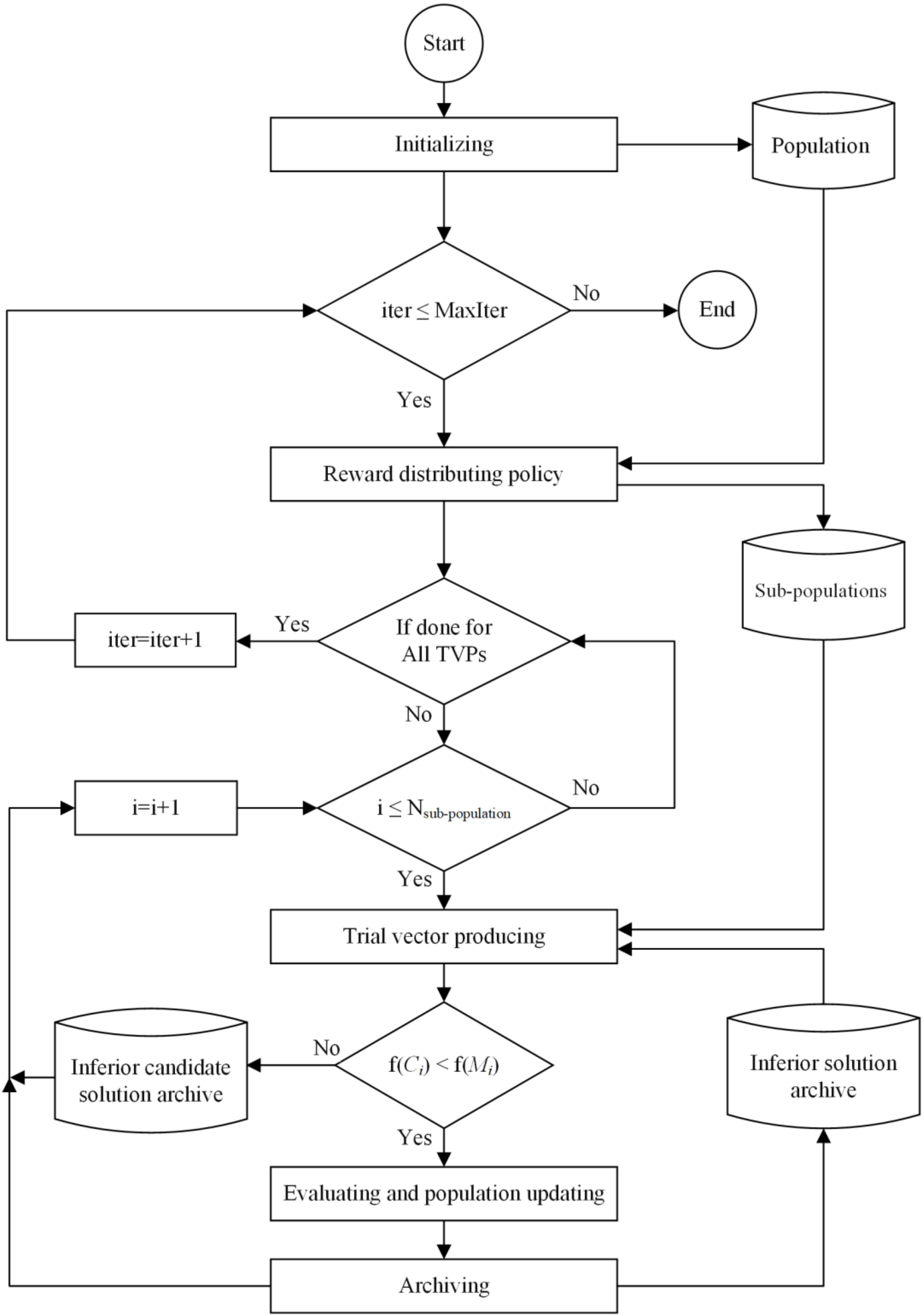
As depicted in Figure 1, the proposed MTV-MFO algorithm consists of four steps: initializing, winner-based distributing, multi-trial vector producing, and evaluating and population updating. After initialization of N moths in the search space, the sub-population size of each TVP is calculated in every nIter iteration, and the moths are relocated by one of the three TVPs. During the evaluation and population updating step of the proposed algorithm, the inferior solution archive and inferior candidate solution archive preserve the subordinate moths in order to use their knowledge leading the existing moths in the population. To lead the moths across the search space, three TVPs are considered in the multi-trial vector producing step; they are moth-flame trial vector producer (MFO-TVP), flag-guided trial vector producer (F-TVP), and contingent trial vector producer (C-TVP). The combination of these TVPs promotes the detection of promising regions by the MTV-MFO algorithm when solving different problems. Table 1 provides the nomenclature for the parameter descriptions used in the following section.
Initializing step: N moths are randomly generated in the search space within the lower (l) and upper (u) bounds using Equation (4).
where Mij is the ith moth’s position in the jth dimension, lj and uj are the minimum and maximum limits of the jth dimension, and rand is a uniformly distributed random variable between 0 and 1, respectively. The moth’s position is stored in matrix M, which has N rows and Dim columns. Additionally, matrix M is replicated in matrix F, which reserves the position of flames. The fitness value of moth Mi is calculated in the tth iteration by the fitness function, f (Mi (t)).
The winner-based distributing step: In every nIter iteration, for the population distribution between three TVPs, the size of the sub-population is determined by calculating the improved rate shown by ImpRate. For each TVP, ImpRate indicates the ratio of the number of improved moths by considering their fitness to the number of function evaluations in the previous nIter iterations. For each TVP, the improved rate is calculated using Equation (5),
where ImpRateMFO-TVP, ImpRateF-TVP, and ImpRateC-TVP are the improved rates, NMFO-TVP, NF-TVP, and NC-TVP are the sub-population size of MFO-TVP, F-TVP, and C-TVP, and NFEs is the number of function evaluations performed by each TVP in the last nIter, respectively. In the MTV-MFO algorithm, the reward rule defined in Equation (6) is considered for distribution policy; thus, the TVP with higher ImpRate has a larger sub-population.
where N is the total number of moths, Nsub-pop is the sub-population’s size by considering the TVPs’ improved rate, and λ is considered 0.25. Then, in this step, three sub-population sizes, NMFO-TVP, NF-TVP, and NC-TVP, are determined, and the sub-populations MMFO-TVP, MF-TVP, and MC-TVP are created.
Multi-trial vector producing step: In each iteration, the position of moth Mi is altered according to the movement strategy of the MFO-TVP, F-TVP, or C-TVP. The MFO-TVP improves the exploitation search ability, which increases the ability to search for new solutions in a small or immediate neighborhood. F-TVP uses a flag flame, spiral movement, gbest is used to exploit and escape the local optima, while C-TVP is adjusted to strike a balance between exploration and exploitation.
Moth-flame trial vector producer (MFO-TVP): In each iteration, MiMFO-TVP, the ith moth from the MFO-TVP’s sub-population, is moved similarly to the mechanism described in the previous section. The distance is calculated by considering the corresponding flame and the logarithmic spiral movement is used to generate the candidate moth. Finally, the MFO-TVP generates the distance and relocates moth MiMFO-TVP by Equations (7) and (8).
where DiMFO-TVP indicates the distance of the ith moth of MMFO-TVP to the jth flame calculated by Equation (3), CiMFO-TVP is the candidate solution provided by logarithmic spiral movement, b is a constant value set to 1, and r is a random number in [−1, 1]. Since the MFO-TVP movement strategy is the same as the MFO movement, this leads to the production of undifferentiated moths over the course of the iterations, which results in undesired premature convergence, imbalanced exploration and exploitation, and degraded results in performance. The pseudo-code of the MFO-TVP is shown in Algorithm 1.
| Algorithm 1. Moth-flame trial vector producer (MFO-TVP). | |
| Input: MMFO-TVP | |
| Output: CMFO-TVP | |
| 1: | Procedure MFO-TVP |
| 2: | For i = 1 to NMFO-TVP |
| 3: | |
| 4: | |
| 5: | End |
| 6: | Return produced vectors in CMFO-TVP |
| 7: | End procedure |
Flag-guided trial vector producer (F-TVP): Meanwhile, the components used in calculating the distance and movement have the main effect on the moths’ position; in F-TVP, the flag flame is introduced with the aim of enhancing the exploration ability. Additionally, the best flame is employed to calculate the distance between moth and flame, and a new spiral function is used to model the flying path of moths. Thus, the distance is calculated by considering the position of the best flame as flag flame to guide the moths. Moreover, in the movement equation of this TVP, the logarithmic spiral shape is changed and a random flame is utilized to form the next position of the moths. The distance and candidate moths are generated by F-TVP according to Equations (9) and (10).
where DiF-TVP indicates the distance of the ith moth of MF-TVP to the best flame of the population Fbest, CiF-TVP is the candidate solution, b is a constant value set to −1, r is a random number in [−1, 1], and Frand is a random flame selected from the entire set of flames. The pseudo-code of the F-TVP is shown in Algorithm 2.
| Algorithm 2. Flag-guided trial vector producer (F-TVP). | |
| Input: MF-TVP | |
| Output: CF-TVP | |
| 1: | Procedure F-TVP |
| 2: | For i = 1 to NF-TVP |
| 3: | |
| 4: | |
| 5: | End |
| 6: | Return produced vectors in CF-TVP |
| 7: | End procedure |
Contingent trial vector producer (C-TVP): C-TVP is introduced to overcome premature convergence and insufficient balance between exploration and exploitation. Thus, two new external archives are employed with the aim of enhancing the population diversity and exploration ability. In addition, the best moth position is considered as the base vector in order to change the moths’ position with respect to the current best moth position. Therefore, the last TVP uses a difference between a random moth from the combination of two archives and the entire moths’ population as shown in Equation (11) and the current moth. The candidate moths are generated by C-TVP according to Equation (12).
where XAll is the union of two archives XInfSolution and XInfCandidate and the entire moths’ population M, Fbest is the best flame’s position in the whole population, FC is a constant value set by 0.7, and CiC-TVP is the candidate solution provided for the ith moth of the MC-TVP. The pseudo-code of the C-TVP is shown in Algorithm 3.
| Algorithm 3. Contingent trial vector producer (C-TVP). | |
| Input: MC-TVP, M, XInfSolution, XInfCandidate | |
| Output: CC-TVP | |
| 1: | Procedure C-TVP |
| 2: | |
| 3: | For i = 1 to NC-TVP |
| 4: | ) |
| 5: | End |
| 6: | Return produced vectors in CC-TVP |
| 7: | End procedure |
Evaluating and population updating: At the end of each iteration, the fitness values of the candidate moths CMFO-TVP, CF-TVP, and CC-TVP are calculated and compared to the previous fitness values of the moths, and the best candidate solutions are permitted for surviving to the next iteration.
Archiving: In each iteration, during the evaluation and population updating step of the MTV-MFO algorithm, two types of inferior moths are obtained. These solutions have salient knowledge about the promising regions of the search space; thus, it is beneficial to store and share their information to guide newly generated moths mostly in the last iterations. Inferior solution archive XInfSolution contains those solutions that are replaced by their candidates. Additionally, inferior candidate solution archive XInfCandidate includes generated candidate solutions that are not eligible for entering the population. At the end of each iteration, the inferior moths (either solution or candidate) are added to the archives, and each archives’ member lifetime variable is increased by one. If the number of archive members exceeds N, then inferior members with a higher lifetime value are randomly removed. By employing these archives during the movement process, good diversity can be maintained in simple and complex functions.
The pseudo-code of the proposed MTV-MFO algorithm is shown in Algorithm 4.
| Algorithm 4. Multi-trial Vector-based Moth-Flame Optimization (MTV-MFO) Algorithm. | |
| Input: N, Dim, MaxIter, nIter | |
| Output: The global optimum (Fbest) | |
| 1: | Begin |
| 2: | iter = 1, Rewarded-TVP = MFO-TVP. |
| 3: | Randomly distribute N moths in the search space. |
| 4: | Evaluating fitness f(Mi) and set the Fbest. |
| 5: | While iter ≤ MaxIter |
| 6: | If mod (iter, nIter) == 0 |
| 7: | Determining ImpRateMFO-TVP, ImpRateF-TVP, and ImpRateC-TVP using Equation 5. |
| 8: | Calculating NMFO-TVP, NF-TVP, and NC-TVP using Equation 6. |
| 9: | End if |
| 10: | Distributing M into MMFO-TVP, MF-TVP, MC-TVP based on reward distributing policy. |
| 11: | Do for each TVP |
| 12: | For i = 1 to Nsub-pop |
| 13: | Multi-trial vector producing. |
| 14: | If f(Ci) < f(Mi) |
| 15: | Updating Mi by Ci and counting the improved moth. |
| 16: | End if |
| 17: | Archiving. |
| 18: | End for |
| 19: | End do |
| 20: | Updating Fbest. |
| 21: | iter = iter + 1. |
| 22: | End while |
| 23: | Return the global optimum (Fbest). |
| 24: | End |
5. Experimental Evaluation and Results
In this section, the proposed MTV-MFO algorithm’s performance is evaluated by a comprehensive experimental study and a statistical analysis. These experiments include exploration and exploitation, local optima avoidance, and convergence evaluation to assess the performance of the MTV-MFO algorithm. The results are compared with the state-of-the-art and recent nature-inspired algorithms, including krill herd (KH) [42], grey wolf optimizer (GWO) [43], moth-flame optimization (MFO) [30] algorithm, whale optimization algorithm (WOA) [7], salp swarm algorithm (SSA) [9], butterfly optimization algorithm (BOA) [44], henry gas solubility optimization (HGSO) [45], and Archimedes optimization algorithm (AOA) [46].
5.1. Benchmark Test Functions and Experimental Environment
The proposed MTV-MFO algorithm was evaluated on 29 test functions of the CEC 2018 benchmark suite [41]. These functions are classified into four categories: unimodal (Func 1, Func 3), simple multimodal (Func 4–Func 10), hybrid (Func 11–Func 20), and composition functions (Func 21–Func 30). The detailed descriptions and mathematical formulations of CEC 2018′s functions are provided in Appendix A. Each category is suitable to assess the ability of algorithms to benchmark the exploitative capability, convergence behavior, exploratory capability, the ability to maintain a balance between exploration and exploitation, and local optima avoidance. Matlab R2018a was used for implementing the MTV-MFO, and the experiments were run on a CPU, Intel Core(TM) i7-3770 3.4GHz and 8.00 GB RAM.
5.2. Experimental Setup
The parameters of all comparative algorithms were set the same as suggested values by their original works, as shown in Table 2. All benchmark functions were evaluated by 20 independent runs with different dimensions of 10, 30, and 50. In each run, the maximum number of iterations (MaxIter) was set by (Dim × 10000)/N where Dim and N were respectively set to the dimensions of the problem and 100. The fitness error value, f(Fbest) − f(X*), was used to report the obtained results, where f(Fbest) is the obtained minimum fitness value and f(X*) is the true global optimum solution of the test function. The mean and standard deviation of the error value were used to measure the performance of the algorithms. The detailed experimental results are shown in Appendix B and in Table A2, Table A3, Table A4 and Table A5, in which the best-obtained error values are marked in boldface, and the overall results are compared in Table 3, Table 4, Table 5 and Table 6. Moreover, the last three rows of each table denoted “w/l/t” indicate the number of wins (w), losses (l), and ties (t) of algorithms.
5.3. Exploration and Exploitation Evaluation
The unimodal functions are particularly used to evaluate the exploitative capability and convergence behavior of the algorithm in those problems that have one optimum, whereas the multimodal functions are suitable to assess the explorative and local optima avoidance abilities of the algorithm. Therefore, by using these two types of test functions, the exploitative and explorative abilities of the MTV-MFO were assessed and compared with comparative algorithms as follows. Table 3 and Table A2 in the Appendix B show that the MTV-MFO algorithm greatly improves MFO results and can provide superior results for unimodal functions in all dimensions 10, 30, and 50. This is mainly because the C-TVP and MFO-TVP movement strategies are mostly exploitative, which helps to escape from possible local optima and maintain diversity. Thus, it can be stated that the MTV-MFO algorithm exploits the optimum solution more effectively than the MFO and other comparative algorithms.
As shown in Table 4 and Table A3, the MTV-MFO can provide superior results on simple multimodal functions on dimensions 10, 30, and 50. The experiment was performed on Func 4–Func 10, where the number of local minima increased exponentially as long as the dimension of the function increased. The overall results on all dimensions show that the MTV-MFO can find superior solutions on seven multimodal functions, while comparative algorithms find unsatisfactory solutions. These results indicate that the proposed MTV-MFO algorithm has better exploration behavior. The main reason for sufficient exploration by the MTV-MFO is mostly because the C-TVP preserves diversity by using archives and explores the search space extensively.
5.4. Evaluation of Local Optima Avoidance
Hybrid and composition functions are defined as more complex and challenging optimization problems because their search landscape is made of multiple unimodal and multimodal functions. Therefore, these functions were suitable to assess the MTV-MFO algorithm’s ability in maintaining the balance of exploration and exploitation, which results in local optima avoidance. The reported results in Table 5 and Table A4 demonstrate that the MTV-MFO on all three dimensions for hybrid functions has superior performance and generates better solutions. Moreover, the overall and detailed results for solving composition functions by the MTV-MFO and other algorithms are reported in Table 6 and Table A5, where the MTV-MFO generates results competitive to those of other, comparative algorithms. Since the MTV-MFO considers the improved rate of each TVP to measure the portion size of sub-populations, an appropriate balance can be achieved between exploration and exploitation. As the results demonstrate, the MTV-MFO obtains a good balance between exploration and exploitation, which improves its local optima avoidance ability.
5.5. Convergence Evaluation
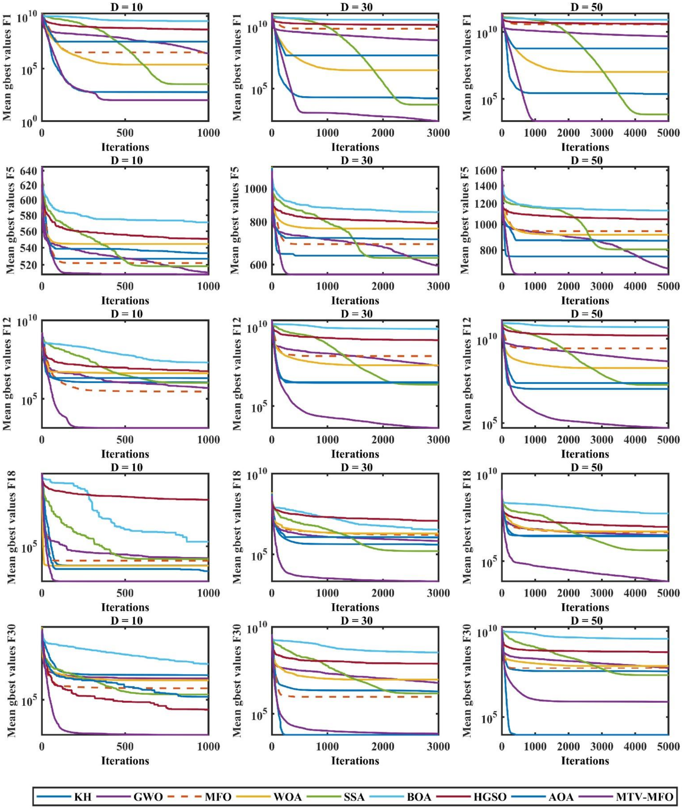
In this experiment, the MTV-MFO convergence behavior and speed were assessed and compared to the comparative algorithms. Figure 2 shows the convergence curves for unimodal function (Func 1), multimodal function (Func 5), hybrid functions (Func 12 and Func 18), and composition function (Func 30) on dimensions 10, 30, and 50. These curves show the mean of best values in every iteration for each algorithm over 20 runs. The MTV-MFO algorithm has a faster convergence on unimodal and multimodal functions. The main reason for sufficient exploitation and exploration of the proposed algorithm is using the combination of best-obtained solutions by three TVPs during the optimization. Additionally, the convergence curves indicate the superiority of the MTV-MFO algorithm on the hybrid and composition functions. The results verify that the MTV-MFO algorithm properly provides a balance between exploration and exploitation in hybrid and composition functions. In addition, it preserves diversity, which can handle difficulties in complex functions.
To summarize the results gained by the performance evaluation, Table 7 shows the overall effectiveness (OE) of the MTV-MFO and comparative algorithms based on their total performance results shown in Table 3, Table 4, Table 5 and Table 6. The algorithms’ OE is calculated using Equation (13), where the parameters N and L are the numbers of functions and the total number of loser functions for each algorithm, respectively.
6. Statistical Analysis
In this section, statistical analyses including Friedman and Student’s t-tests were performed to show the significant difference between the results obtained for the MTV-MFO and comparative algorithms. To ensure a fair comparison, all analyses were run on Matlab R2018a.
6.1. Friedman Test
Although the experimental evaluation results compare the proposed MTV-MFO algorithm and comparative algorithms’ overall performance, the algorithms’ statistical significance was not determined. Then, the non-parametric test Friedman was conducted to prove the superiority of the MTV-MFO statistically. The Friedman test (Ff) [94] is a non-parametric test used for multiple comparisons of different algorithms for all functions. This test was used to rank the MTV-MFO and comparative algorithms based on the achieved fitness by using Equation (14),
where k, n, and Rj are the number of algorithms, case tests, and the mean rank of the jth algorithm, respectively. For each pair of algorithms, it ranks from 1 (best result) to k (worst result), then calculates the average ranks obtained in all problems to obtain the final rank of each algorithm. Based on the Friedman test results tabulated in Table 8, the overall ranking proved the MTV-MFO algorithm’s superiority compared with other state-of-the-art algorithms on dimensions 10, 30, and 50.
6.2. Student’s t-Test
In order to verify if there was a significant difference between the gained results between the proposed algorithm and the comparative algorithms, the pairwise student’s t-test was used. The null hypothesis, H0, states that the average best value for both compared algorithms is the same unless the two values are different, which shows the alternative hypothesis H1. In Table 9, the results of this pairwise statistical test are demonstrated with a 5% significance level. The gained results show the superiority of the MTV-MFO algorithm in comparison with other state-of-the-art algorithms on dimensions 10, 30, and 50, while in most functions the MTV-MFO algorithm obtained t-test values greater than 1.
6.3. Box Plot Analysis
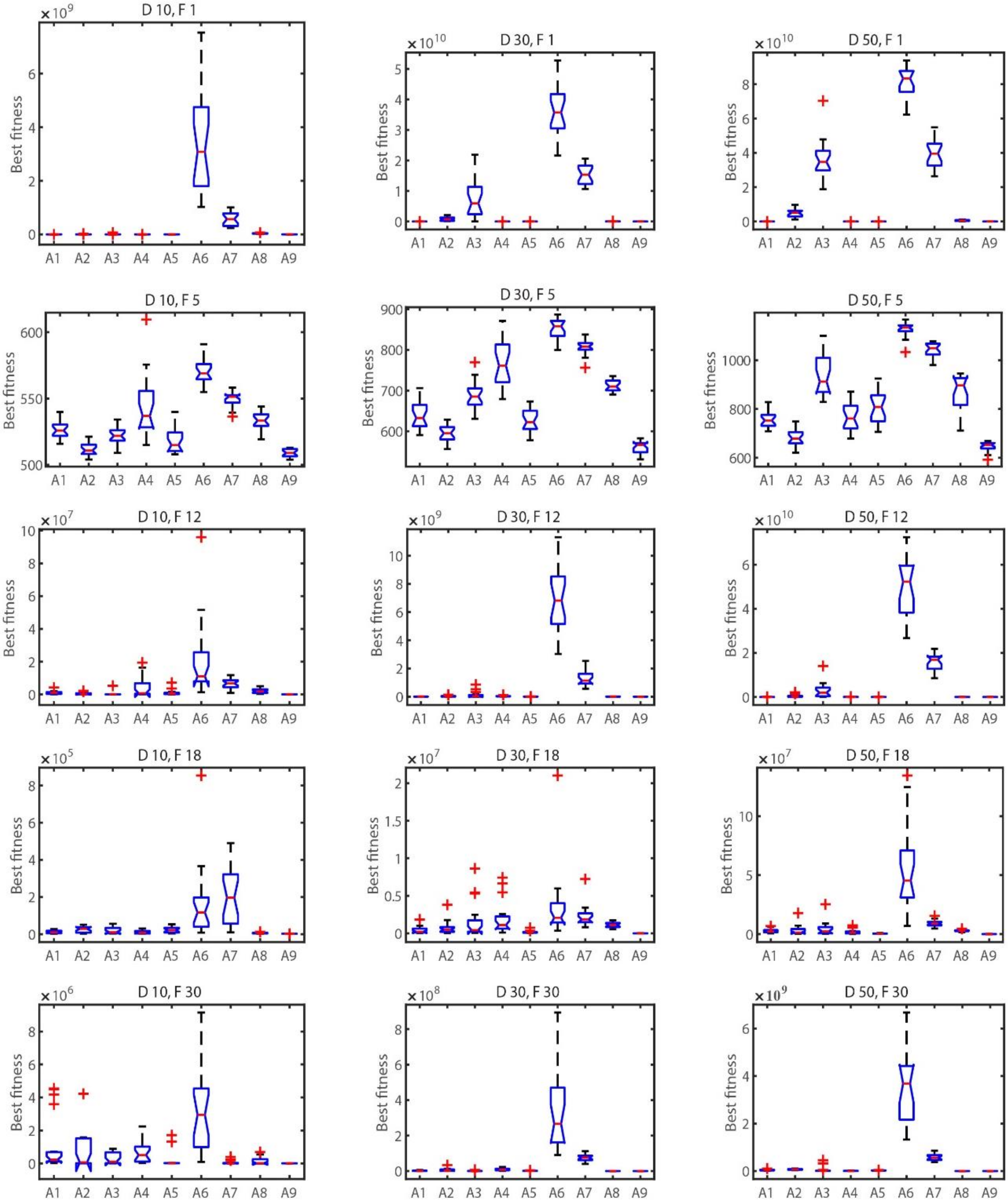
A box plot analysis was performed to investigate the distributional aspects of the experiments in previous subsections; boxplots for selected functions on dimensions 10, 30, and 50 are illustrated in Figure 3. The best-gained values for each function from 20 runs were used for this analysis. The box plot shows the dispersion and symmetry of the gained results while illustrating the distribution of the results. The first, second (median), third, and lower quartiles, upper limits, and outliers are shown by a box plot. The larger the rectangular box, the more dispersed the results are, and the algorithm’s gained results are unstable. It also represents the performance that is the weakest in comparison. The median of data sets is indicated by the red crossbar, and outliers are indicated by the plus sign (+) in red. The boxplot analysis confirms the consistent ability of the MTV-MFO algorithm in searching for the optimal solution, and also proves its ability to gain better results overall.
7. Conclusions and Future Works
Swarm-intelligence metaheuristic algorithms are well-known stochastic algorithms that are used to solve different optimization problems including non-linear, non-differentiable, and non-convex problems; however, there are flaws in the algorithms when solving complex problems. In this article, we used the multi-trial vector approach to propose a multi-trial vector-based moth-flame optimization (MTV-MFO) algorithm, which is an enhancement for the moth-flame optimization (MFO) algorithm. The movement strategy of the MFO leads to premature convergence and insufficient balance between exploration and exploitation. Therefore, the MFO’s movement strategy was substituted by the MTV approach to use a combination of different TVPs. In the MTV approach, the whole population is distributed based on the winner-based distribution policy to a number of sub-populations, such that each sub-population has its own TVP. The main advantages of the MTV-MFO are using two strategies, flag-guided trial vector producer (F-TVP) and contingent trial vector producer (C-TVP), which cooperate with the canonical moth-flame trial vector producer (MFO-TVP) to handle different problems with diverse characteristics. Furthermore, the MTV-MFO algorithm uses the knowledge of inferior moths preserved in two archives to prevent premature convergence and avoid local optima. The statistical analysis results revealed a significant difference between the results of the proposed algorithm and other comparative algorithms. From the results gained by experimental performance evaluation and statistical analysis, the conclusions can be stated as follows:
- -
- The proposed F-TVP and C-TVP enhance exploitation and exploitation.
- -
- Cooperation of the proposed F-TVP and C-TVP with the canonical MFO-TVP enhances the balance between exploration and exploitation, which enables the MTV-MFO algorithm to escape from the local optima.
- -
- The results obtained from different experiments on diverse test functions with various characteristics and statistical tests verify the performance of the MTV-MFO algorithm in comparison to other, comparative algorithms.
The MTV-MFO algorithm is designed to optimize single-objective continuous problems, and it can be extended to solve binary problems and developed for multi-objective problems. Furthermore, the MTV-MFO algorithm can be applied to solve real-world optimization problems in electrical networks, structural engineering such as load balancing, scheduling, resource distribution, and vehicle routing.
Author Contributions
Conceptualization, M.H.N.-S.; Methodology, M.H.N.-S. and S.T.; Software, M.H.N.-S. and S.T.; Validation, M.H.N.-S., S.T., S.M., L.A., M.A.E. and A.A.E.; Formal analysis, M.H.N.-S. and S.T.; Investigation, M.H.N.-S. and S.T.; Resources, M.H.N.-S., S.T. and S.M.; Data curation, M.H.N.-S. and S.T.; Writing, M.H.N.-S. and S.T.; Original draft preparation, M.H.N.-S. and S.T.; Writing—review and editing, M.H.N.-S., S.T., S.M., L.A., M.A.E. and A.A.E.; Visualization, M.H.N.-S. and S.T.; Supervision, M.H.N.-S. and S.M.; Project administration, M.H.N.-S. and S.M. All authors have read and agreed to the published version of the manuscript.
Funding
This research received no external funding.
Institutional Review Board Statement
Not applicable.
Informed Consent Statement
Not applicable.
Data Availability Statement
Not applicable.
Conflicts of Interest
The authors declare no conflict of interest.
Appendix A
The detailed descriptions and mathematical formulations of CEC 2018′s functions are provided in Table A1.

Table A1.
Description of benchmark functions from CEC 2018.
| Function | Name and Formulation | Fi* = Fi(x*) |
|---|---|---|
| Func 1 | Shifted and Rotated Bent Cigar Function | 100 |
| Func 3 | Shifted and Rotated Zakharov Function | 300 |
| Func 4 | Shifted and Rotated Rosenbrock’s Function | 400 |
| Func 5 | Shifted and Rotated Rastrigin’s Function | 500 |
| Func 6 | Shifted and Rotated Expanded Scaffer’s F6 Function | 600 |
| Func 7 | Shifted and Rotated Lunacek Bi_Rastrigin Function , , for i = 1,2,…,D | 700 |
| Func 8 | Shifted and Rotated Non-Continuous Rastrigin’s Function for i = 1,2,…, D , i = 1,2,…,D. , for i=1,…,D | 800 |
| Func 9 | Shifted and Rotated Levy Function | 900 |
| Func 10 | Shifted and Rotated Schwefel’s Function | 1000 |
| Func 11 | Hybrid Function 1 (N = 3) | 1100 |
| Func 12 | Hybrid Function 2 (N = 3) | 1200 |
| Func 13 | Hybrid Function 3 (N = 3) | 1300 |
| Func 14 | Hybrid Function 4 (N = 4) | 1400 |
| Func 15 | Hybrid Function 5 (N = 4) | 1500 |
| Func 16 | Hybrid Function 6 (N = 4) | 1600 |
| Func 17 | Hybrid Function 6 (N = 5) | 1700 |
| Func 18 | Hybrid Function 6 (N = 5) | 1800 |
| Func 19 | Hybrid Function 6 (N = 5) | 1900 |
| Func 20 | Hybrid Function 6 (N = 6) | 2000 |
| Func 21 | Composition Function 1 (N = 3) ’ | 2100 |
| Func 22 | Composition Function 2 (N = 3) ’ | 2200 |
| Func 23 | Composition Function 3 (N = 4) ’ | 2300 |
| Func 24 | Composition Function 4 (N = 4) ’ | 2400 |
| Func 25 | Composition Function 5 (N = 5) ’ | 2500 |
| Func 26 | Composition Function 6 (N = 5) ’ | 2600 |
| Func 27 | Composition Function 7 (N = 6) ’ | 2700 |
| Func 28 | Composition Function 8 (N = 6) ’ | 2800 |
| Func 29 | Composition Function 9 (N = 3) ’ | 2900 |
| Func 30 | Composition Function 10 (N = 3) ’ | 3000 |
Appendix B
The detailed results for the unimodal, multimodal, hybrid, and composition functions of CEC 2018 for the proposed MTV-MFO algorithm and comparative algorithms are provided in Table A2, Table A3, Table A4 and Table A5.
Table A2.
The obtained results for unimodal test functions.
| Func | Dim | Metric | KH (2012) | GWO (2014) | MFO (2015) | WOA (2016) | SSA (2017) | BOA (2019) | HGSO (2019) | AOA (2020) | MTV-MFO |
|---|---|---|---|---|---|---|---|---|---|---|---|
| Func 1 | 10 | Avg | 4.81 × 10² | 2.69 × 10⁶ | 3.51 × 10⁶ | 2.37 × 10⁵ | 3.17 × 10³ | 9.77 × 10⁹ | 5.64 × 10⁸ | 3.64 × 10⁷ | 0 |
| SD | 5.15 × 10² | 7.21 × 10⁶ | 1.57 × 10⁷ | 4.36 × 10⁵ | 2.96 × 10³ | 2.39 × 10⁹ | 2.52 × 10⁸ | 1.23 × 10⁷ | 0 | ||
| Min | 3.00 × 101 | 5.00 × 10³ | 3.15 × 101 | 1.36 × 10⁴ | 4.58 × 100 | 3.62 × 10⁹ | 2.39 × 10⁸ | 1.64 × 10⁷ | 0 | ||
| 30 | Avg | 1.59 × 10⁴ | 8.15 × 10⁸ | 6.85 × 10⁹ | 3.01 × 10⁶ | 4.86 × 10³ | 5.62 × 10¹⁰ | 1.52 × 10¹⁰ | 4.79 × 10⁷ | 1.33 × 10² | |
| SD | 1.44 × 10⁴ | 6.24 × 10⁸ | 5.86 × 10⁹ | 2.24 × 10⁶ | 5.76 × 10³ | 5.04 × 10⁹ | 3.24 × 10⁹ | 2.37 × 10⁷ | 1.43 × 10² | ||
| Min | 2.86 × 10³ | 1.60 × 10⁸ | 5.49 × 10³ | 7.79 × 10⁵ | 5.58 × 101 | 4.75 × 10¹⁰ | 1.07 × 10¹⁰ | 1.72 × 10⁷ | 3.53 × 10⁻² | ||
| 50 | Avg | 2.31 × 10⁵ | 4.74 × 10⁹ | 3.64 × 10¹⁰ | 1.02 × 10⁷ | 6.71 × 10³ | 1.07 × 10¹¹ | 3.95 × 10¹⁰ | 5.69 × 10⁸ | 2.06 × 10³ | |
| SD | 1.70 × 10⁵ | 2.11 × 10⁹ | 1.10 × 10¹⁰ | 1.06 × 10⁷ | 8.58 × 10³ | 5.19 × 10⁹ | 8.59 × 10⁹ | 3.09 × 10⁸ | 1.52 × 10³ | ||
| Min | 6.31 × 10⁴ | 1.19 × 10⁹ | 1.87 × 10¹⁰ | 2.86 × 10⁶ | 9.38 × 100 | 9.43 × 10¹⁰ | 2.64 × 10¹⁰ | 2.29 × 10⁸ | 8.40 × 100 | ||
| Func 3 | 10 | Avg | 9.01 × 10² | 5.33 × 10² | 3.41 × 10³ | 1.68 × 10² | 1.17 × 10⁻⁹ | 1.35 × 10⁴ | 7.31 × 10² | 1.81 × 10³ | 0 |
| SD | 1.13 × 10³ | 8.25 × 10² | 5.53 × 10³ | 1.52 × 10² | 4.43 × 10¹⁰ | 2.86 × 10³ | 3.07 × 10² | 1.02 × 10³ | 0 | ||
| Min | 2.85 × 101 | 2.52 × 101 | 0 | 3.79 × 100 | 3.37 × 10¹⁰ | 8.42 × 10³ | 3.40 × 10² | 3.19 × 10² | 0 | ||
| 30 | Avg | 4.53 × 10⁴ | 2.62 × 10⁴ | 8.80 × 10⁴ | 1.54 × 10⁵ | 3.61 × 10⁻⁸ | 8.30 × 10⁴ | 3.84 × 10⁴ | 4.15 × 10⁴ | 0 | |
| SD | 1.41 × 10⁴ | 7.06 × 10³ | 4.64 × 10⁴ | 7.27 × 10⁴ | 1.10 × 10⁻⁸ | 8.16 × 10³ | 7.17 × 10³ | 1.01 × 10⁴ | 0 | ||
| Min | 2.66 × 10⁴ | 9.68 × 10³ | 1.18 × 10⁴ | 4.94 × 10⁴ | 2.49 × 10⁻⁸ | 6.44 × 10⁴ | 2.11 × 10⁴ | 2.15 × 10⁴ | 0 | ||
| 50 | Avg | 1.15 × 10⁵ | 6.76 × 10⁴ | 1.89 × 10⁵ | 6.98 × 10⁴ | 1.96 × 10⁻⁷ | 2.35 × 10⁵ | 1.39 × 10⁵ | 1.01 × 10⁵ | 0 | |
| SD | 2.23 × 10⁴ | 1.55 × 10⁴ | 9.49 × 10⁴ | 2.77 × 10⁴ | 5.46 × 10⁻⁸ | 5.73 × 10⁴ | 8.39 × 10³ | 1.10 × 10⁴ | 0 | ||
| Min | 8.23 × 10⁴ | 4.21 × 10⁴ | 1.44 × 10⁴ | 3.65 × 10⁴ | 1.28 × 10⁻⁷ | 1.78 × 10⁵ | 1.26 × 10⁵ | 8.24 × 10⁴ | 0 | ||
| Rank | 10 | (w/l/t) | 0/2/0 | 0/2/0 | 0/2/0 | 0/2/0 | 0/2/0 | 0/2/0 | 0/2/0 | 0/2/0 | 2/0/0 |
| 30 | (w/l/t) | 0/2/0 | 0/2/0 | 0/2/0 | 0/2/0 | 0/2/0 | 0/2/0 | 0/2/0 | 0/2/0 | 2/0/0 | |
| 50 | (w/l/t) | 0/2/0 | 0/2/0 | 0/2/0 | 0/2/0 | 0/2/0 | 0/2/0 | 0/2/0 | 0/2/0 | 2/0/0 |
Func: function, Dim: dimension, Avg: mean, SD: standard deviation, Min: minimum error value, w: wins, l: losses, t: ties.
Table A3.
The obtained results for simple multimodal test functions.
| Func | Dim | Metric | KH (2012) | GWO (2014) | MFO (2015) | WOA (2016) | SSA (2017) | BOA (2019) | HGSO (2019) | AOA (2020) | MTV-MFO |
|---|---|---|---|---|---|---|---|---|---|---|---|
| Func 4 | 10 | Avg | 5.91 × 100 | 7.85 × 100 | 5.48 × 100 | 4.01 × 101 | 3.97 × 100 | 1.24 × 10³ | 4.65 × 101 | 1.80 × 101 | 0 |
| SD | 2.42 × 100 | 2.76 × 100 | 2.67 × 100 | 4.52 × 101 | 1.55 × 100 | 3.21 × 10² | 1.28 × 101 | 1.42 × 101 | 0 | ||
| Min | 1.18 × 10⁻¹ | 6.17 × 100 | 1.15 × 100 | 3.05 × 100 | 8.81 × 10⁻³ | 6.26 × 10² | 2.33 × 101 | 7.86 × 100 | 0 | ||
| 30 | Avg | 9.87 × 101 | 1.59 × 10² | 5.10 × 10² | 1.58 × 10² | 8.71 × 101 | 2.12 × 10⁴ | 1.63 × 10³ | 1.28 × 10² | 7.42 × 10⁻¹ | |
| SD | 2.03 × 101 | 4.16 × 101 | 4.00 × 10² | 3.94 × 101 | 1.71 × 101 | 3.62 × 10³ | 4.48 × 10² | 2.01 × 101 | 1.41 × 100 | ||
| Min | 6.83 × 101 | 9.85 × 101 | 9.92 × 101 | 1.13 × 10² | 3.70 × 101 | 1.15 × 10⁴ | 1.06 × 10³ | 1.02 × 10² | 1.70 × 10⁻³ | ||
| 50 | Avg | 1.54 × 10² | 4.42 × 10² | 2.78 × 10³ | 2.82 × 10² | 1.41 × 10² | 4.16 × 10⁴ | 7.71 × 10³ | 3.48 × 10² | 6.16 × 101 | |
| SD | 5.06 × 101 | 1.86 × 10² | 2.48 × 10³ | 6.46 × 101 | 5.08 × 101 | 5.30 × 10³ | 1.78 × 10³ | 7.15 × 101 | 3.82 × 101 | ||
| Min | 7.32 × 101 | 2.08 × 10² | 4.46 × 10² | 2.10 × 10² | 3.25 × 101 | 3.24 × 10⁴ | 4.51 × 10³ | 2.00 × 10² | 5.74 × 10⁻² | ||
| Func 5 | 10 | Avg | 2.69 × 101 | 1.14 × 101 | 2.20 × 101 | 4.44 × 101 | 1.85 × 101 | 1.18 × 10² | 4.97 × 101 | 3.35 × 101 | 8.95 × 100 |
| SD | 7.13 × 100 | 4.41 × 100 | 5.47 × 100 | 2.26 × 101 | 9.29 × 100 | 1.35 × 101 | 5.38 × 100 | 6.49 × 100 | 2.96 × 100 | ||
| Min | 1.59 × 101 | 4.08 × 100 | 8.95 × 100 | 1.50 × 101 | 7.96 × 100 | 9.06 × 101 | 3.64 × 101 | 1.93 × 101 | 3.98 × 100 | ||
| 30 | Avg | 1.37 × 10² | 9.53 × 101 | 1.88 × 10² | 2.64 × 10² | 1.27 × 10² | 5.86 × 10² | 3.06 × 10² | 2.11 × 10² | 6.13 × 101 | |
| SD | 3.14 × 101 | 2.03 × 101 | 3.29 × 101 | 5.56 × 101 | 2.96 × 101 | 4.66 × 101 | 1.71 × 101 | 1.45 × 101 | 1.51 × 101 | ||
| Min | 9.06 × 101 | 5.58 × 101 | 1.31 × 10² | 1.79 × 10² | 7.76 × 101 | 5.05 × 10² | 2.56 × 10² | 1.90 × 10² | 3.08 × 101 | ||
| 50 | Avg | 2.56 × 10² | 1.81 × 10² | 4.43 × 10² | 4.13 × 10² | 3.04 × 10² | 9.51 × 10² | 5.45 × 10² | 3.68 × 10² | 1.47 × 10² | |
| SD | 3.11 × 101 | 3.45 × 101 | 8.55 × 101 | 8.06 × 101 | 6.46 × 101 | 5.18 × 101 | 2.80 × 101 | 7.74 × 101 | 2.08 × 101 | ||
| Min | 2.09 × 10² | 1.21 × 10² | 3.29 × 10² | 2.73 × 10² | 2.06 × 10² | 8.18 × 10² | 4.80 × 10² | 2.11 × 10² | 9.25 × 101 | ||
| Func 6 | 10 | Avg | 5.40 × 100 | 1.19 × 100 | 4.21 × 10⁻¹ | 3.15 × 101 | 6.38 × 100 | 6.51 × 101 | 2.43 × 101 | 9.41 × 10⁻¹ | 0 |
| SD | 6.81 × 100 | 1.52 × 100 | 7.00 × 10⁻¹ | 1.28 × 101 | 7.55 × 100 | 1.38 × 101 | 4.30 × 100 | 4.36 × 10⁻¹ | 0 | ||
| Min | 3.86 × 10⁻⁵ | 2.51 × 10⁻² | 0 | 1.28 × 101 | 2.72 × 10⁻² | 4.37 × 101 | 1.60 × 101 | 2.70 × 10⁻¹ | 0 | ||
| 30 | Avg | 3.55 × 101 | 5.24 × 100 | 2.82 × 101 | 6.93 × 101 | 3.12 × 101 | 1.17 × 10² | 6.48 × 101 | 8.75 × 100 | 1.34 × 10⁻¹ | |
| SD | 9.06 × 100 | 2.81 × 100 | 1.44 × 101 | 9.73 × 100 | 1.32 × 101 | 1.24 × 101 | 6.35 × 100 | 2.63 × 100 | 1.07 × 10⁻¹ | ||
| Min | 1.95 × 101 | 8.70 × 10⁻¹ | 7.63 × 100 | 5.02 × 101 | 9.19 × 100 | 8.83 × 101 | 4.73 × 101 | 5.06 × 100 | 1.49 × 10⁻² | ||
| 50 | Avg | 5.13 × 101 | 1.10 × 101 | 4.76 × 101 | 7.54 × 101 | 4.34 × 101 | 1.32 × 10² | 8.24 × 101 | 2.06 × 101 | 4.70 × 100 | |
| SD | 6.46 × 100 | 3.96 × 100 | 6.44 × 100 | 9.30 × 100 | 9.48 × 100 | 7.76 × 100 | 4.74 × 100 | 4.14 × 100 | 2.41 × 100 | ||
| Min | 3.74 × 101 | 5.12 × 100 | 3.66 × 101 | 6.58 × 101 | 2.40 × 101 | 1.18 × 10² | 7.14 × 101 | 1.46 × 101 | 6.24 × 10⁻¹ | ||
| Func 7 | 10 | Avg | 2.10 × 101 | 2.52 × 101 | 3.58 × 101 | 7.61 × 101 | 3.46 × 101 | 3.21 × 10² | 6.63 × 101 | 3.77 × 101 | 1.80 × 101 |
| SD | 5.34 × 100 | 8.53 × 100 | 1.17 × 101 | 3.26 × 101 | 1.25 × 101 | 6.53 × 101 | 7.30 × 100 | 5.29 × 100 | 4.04 × 100 | ||
| Min | 1.26 × 101 | 1.46 × 101 | 1.48 × 101 | 2.71 × 101 | 2.00 × 101 | 1.82 × 10² | 4.52 × 101 | 2.99 × 101 | 7.78 × 100 | ||
| 30 | Avg | 1.33 × 10² | 1.53 × 10² | 3.27 × 10² | 5.04 × 10² | 1.64 × 10² | 1.15 × 10³ | 4.01 × 10² | 2.44 × 10² | 1.16 × 10² | |
| SD | 2.64 × 101 | 4.96 × 101 | 1.22 × 10² | 1.01 × 10² | 3.09 × 101 | 1.17 × 10² | 3.32 × 101 | 1.37 × 101 | 1.30 × 101 | ||
| Min | 8.34 × 101 | 9.08 × 101 | 1.56 × 10² | 3.35 × 10² | 1.11 × 10² | 9.01 × 10² | 3.24 × 10² | 2.15 × 10² | 9.23 × 101 | ||
| 50 | Avg | 3.62 × 10² | 3.38 × 10² | 9.72 × 10² | 1.01 × 10³ | 3.36 × 10² | 1.86 × 10³ | 8.29 × 10² | 5.15 × 10² | 2.82 × 10² | |
| SD | 5.66 × 101 | 8.31 × 101 | 3.07 × 10² | 1.01 × 10² | 9.21 × 101 | 1.28 × 10² | 6.43 × 101 | 3.84 × 101 | 3.84 × 101 | ||
| Min | 2.74 × 10² | 2.07 × 10² | 4.02 × 10² | 7.66 × 10² | 2.18 × 10² | 1.66 × 10³ | 7.17 × 10² | 4.31 × 10² | 1.93 × 10² | ||
| Func 8 | 10 | Avg | 1.63 × 101 | 1.04 × 101 | 2.48 × 101 | 4.05 × 101 | 1.73 × 101 | 1.04 × 10² | 3.21 × 101 | 2.34 × 101 | 1.02 × 101 |
| SD | 6.96 × 100 | 3.67 × 100 | 1.12 × 101 | 1.58 × 101 | 9.37 × 100 | 1.32 × 101 | 3.30 × 100 | 5.24 × 100 | 3.41 × 100 | ||
| Min | 7.96 × 100 | 5.97 × 100 | 4.97 × 100 | 2.09 × 101 | 4.97 × 100 | 7.63 × 101 | 2.67 × 101 | 1.36 × 101 | 1.99 × 100 | ||
| 30 | Avg | 1.09 × 10² | 7.73 × 101 | 1.67 × 10² | 2.16 × 10² | 1.19 × 10² | 4.82 × 10² | 2.53 × 10² | 1.89 × 10² | 7.27 × 101 | |
| SD | 1.69 × 101 | 2.83 × 101 | 3.83 × 101 | 5.54 × 101 | 2.72 × 101 | 3.62 × 101 | 1.36 × 101 | 1.55 × 101 | 1.07 × 101 | ||
| Min | 7.36 × 101 | 4.22 × 101 | 9.11 × 101 | 1.28 × 10² | 8.36 × 101 | 4.22 × 10² | 2.27 × 10² | 1.57 × 10² | 5.07 × 101 | ||
| 50 | Avg | 2.84 × 10² | 2.02 × 10² | 3.97 × 10² | 4.11 × 10² | 2.89 × 10² | 9.91 × 10² | 5.71 × 10² | 3.59 × 10² | 1.28 × 10² | |
| SD | 4.77 × 101 | 3.18 × 101 | 7.78 × 101 | 7.29 × 101 | 8.11 × 101 | 5.42 × 101 | 2.75 × 101 | 9.00 × 101 | 2.10 × 101 | ||
| Min | 2.09 × 10² | 1.36 × 10² | 2.69 × 10² | 2.93 × 10² | 1.93 × 10² | 8.76 × 10² | 5.03 × 10² | 2.18 × 10² | 8.16 × 101 | ||
| Func 9 | 10 | Avg | 8.52 × 100 | 6.17 × 100 | 3.79 × 101 | 4.52 × 10² | 4.79 × 100 | 2.54 × 10³ | 9.80 × 101 | 3.81 × 100 | 0 |
| SD | 2.28 × 101 | 1.58 × 101 | 1.53 × 10² | 3.37 × 10² | 1.80 × 101 | 6.69 × 10² | 2.43 × 101 | 2.71 × 100 | 0 | ||
| Min | 3.35 × 10⁻⁵ | 4.93 × 10⁻² | 0 | 4.81 × 101 | 1.36 × 10¹⁰ | 1.13 × 10³ | 4.46 × 101 | 1.02 × 100 | 0 | ||
| 30 | Avg | 2.31 × 10³ | 5.29 × 10² | 4.68 × 10³ | 6.42 × 10³ | 2.23 × 10³ | 2.69 × 10⁴ | 4.98 × 10³ | 9.96 × 10² | 1.50 × 10² | |
| SD | 6.62 × 10² | 3.60 × 10² | 1.55 × 10³ | 2.04 × 10³ | 1.24 × 10³ | 4.98 × 10³ | 9.90 × 10² | 3.18 × 10² | 9.61 × 101 | ||
| Min | 9.31 × 10² | 8.54 × 101 | 2.82 × 10³ | 2.72 × 10³ | 4.25 × 101 | 1.65 × 10⁴ | 3.17 × 10³ | 5.03 × 10² | 9.80 × 100 | ||
| 50 | Avg | 9.41 × 10³ | 4.49 × 10³ | 1.47 × 10⁴ | 2.01 × 10⁴ | 1.01 × 10⁴ | 7.99 × 10⁴ | 2.61 × 10⁴ | 1.02 × 10⁴ | 1.26 × 10³ | |
| SD | 1.36 × 10³ | 3.26 × 10³ | 3.08 × 10³ | 6.78 × 10³ | 2.22 × 10³ | 5.95 × 10³ | 2.02 × 10³ | 1.93 × 10³ | 4.98 × 10² | ||
| Min | 7.64 × 10³ | 1.51 × 10³ | 7.99 × 10³ | 1.24 × 10⁴ | 6.49 × 10³ | 6.85 × 10⁴ | 2.05 × 10⁴ | 7.01 × 10³ | 4.15 × 10² | ||
| Func 10 | 10 | Avg | 9.94 × 10² | 5.21 × 10² | 7.37 × 10² | 9.41 × 10² | 9.15 × 10² | 2.24 × 10³ | 1.36 × 10³ | 1.05 × 10³ | 4.06 × 10² |
| SD | 2.88 × 10² | 3.13 × 10² | 2.73 × 10² | 2.47 × 10² | 2.60 × 10² | 2.16 × 10² | 1.82 × 10² | 2.51 × 10² | 1.28 × 10² | ||
| Min | 4.56 × 10² | 4.14 × 101 | 3.14 × 10² | 4.81 × 10² | 2.99 × 10² | 1.73 × 10³ | 8.50 × 10² | 5.36 × 10² | 1.34 × 10² | ||
| 30 | Avg | 4.06 × 10³ | 3.25 × 10³ | 4.23 × 10³ | 5.18 × 10³ | 3.60 × 10³ | 8.93 × 10³ | 5.72 × 10³ | 6.60 × 10³ | 3.08 × 10³ | |
| SD | 4.36 × 10² | 9.30 × 10² | 7.04 × 10² | 7.27 × 10² | 5.51 × 10² | 3.18 × 10² | 3.44 × 10² | 4.75 × 10² | 5.31 × 10² | ||
| Min | 3.37 × 10³ | 1.77 × 10³ | 2.98 × 10³ | 3.83 × 10³ | 2.75 × 10³ | 8.24 × 10³ | 5.10 × 10³ | 5.61 × 10³ | 1.97 × 10³ | ||
| 50 | Avg | 6.65 × 10³ | 5.45 × 10³ | 7.32 × 10³ | 8.87 × 10³ | 6.47 × 10³ | 1.56 × 10⁴ | 1.17 × 10⁴ | 1.32 × 10⁴ | 5.36 × 10³ | |
| SD | 8.55 × 10² | 7.81 × 10² | 1.09 × 10³ | 1.13 × 10³ | 1.03 × 10³ | 4.33 × 10² | 6.84 × 10² | 4.13 × 10² | 4.48 × 10² | ||
| Min | 5.33 × 10³ | 3.91 × 10³ | 4.94 × 10³ | 7.22 × 10³ | 4.81 × 10³ | 1.49 × 10⁴ | 1.08 × 10⁴ | 1.26 × 10⁴ | 4.92 × 10³ | ||
| Rank | 10 | (w/l/t) | 0/7/0 | 0/7/0 | 0/7/0 | 0/7/0 | 0/7/0 | 0/7/0 | 0/7/0 | 0/7/0 | 7/0/0 |
| 30 | (w/l/t) | 0/7/0 | 0/7/0 | 0/7/0 | 0/7/0 | 0/7/0 | 0/7/0 | 0/7/0 | 0/7/0 | 7/0/0 | |
| 50 | (w/l/t) | 0/7/0 | 0/7/0 | 0/7/0 | 0/7/0 | 0/7/0 | 0/7/0 | 0/7/0 | 0/7/0 | 7/0/0 |
Func: function, Dim: dimension, Avg: mean, SD: standard deviation, Min: minimum error value, w: wins, l: losses, t: ties.
Table A4.
The obtained results for hybrid test functions.
| Func | Dim | Metric | KH (2012) | GWO (2014) | MFO (2015) | WOA (2016) | SSA (2017) | BOA (2019) | HGSO (2019) | AOA (2020) | MTV-MFO |
|---|---|---|---|---|---|---|---|---|---|---|---|
| Func 11 | 10 | Avg | 4.09 × 101 | 1.97 × 101 | 4.13 × 101 | 8.50 × 101 | 9.43 × 101 | 1.70 × 10³ | 1.30 × 10² | 2.11 × 10² | 4.30 × 100 |
| SD | 2.30 × 101 | 9.59 × 100 | 4.78 × 101 | 5.71 × 101 | 7.99 × 101 | 1.34 × 10³ | 4.43 × 101 | 1.05 × 10² | 1.79 × 100 | ||
| Min | 2.67 × 100 | 6.26 × 100 | 3.48 × 100 | 3.02 × 101 | 1.36 × 101 | 2.55 × 10² | 6.00 × 101 | 7.94 × 101 | 9.95 × 10⁻¹ | ||
| 30 | Avg | 4.02 × 10² | 2.30 × 10² | 1.92 × 10³ | 3.52 × 10² | 1.66 × 10² | 7.00 × 10³ | 1.44 × 10³ | 8.34 × 10² | 9.20 × 101 | |
| SD | 1.84 × 10² | 4.87 × 101 | 1.97 × 10³ | 9.76 × 101 | 4.74 × 101 | 1.94 × 10³ | 5.84 × 10² | 3.08 × 10² | 2.32 × 101 | ||
| Min | 1.56 × 10² | 1.40 × 10² | 2.22 × 10² | 1.96 × 10² | 9.11 × 101 | 3.95 × 10³ | 5.80 × 10² | 4.50 × 10² | 5.77 × 101 | ||
| 50 | Avg | 3.56 × 10³ | 1.34 × 10³ | 7.81 × 10³ | 4.69 × 10² | 2.77 × 10² | 2.45 × 10⁴ | 4.89 × 10³ | 9.76 × 10³ | 1.59 × 10² | |
| SD | 1.69 × 10³ | 1.09 × 10³ | 9.73 × 10³ | 1.04 × 10² | 7.45 × 101 | 2.95 × 10³ | 1.25 × 10³ | 1.63 × 10³ | 3.40 × 101 | ||
| Min | 1.29 × 10³ | 3.63 × 10² | 5.38 × 10² | 3.31 × 10² | 1.46 × 10² | 1.70 × 10⁴ | 2.51 × 10³ | 6.82 × 10³ | 1.11 × 10² | ||
| Func 12 | 10 | Avg | 1.10 × 10⁶ | 4.87 × 10⁵ | 2.82 × 10⁵ | 4.21 × 10⁶ | 1.03 × 10⁶ | 4.12 × 10⁸ | 6.48 × 10⁶ | 2.07 × 10⁶ | 1.91 × 10² |
| SD | 9.36 × 10⁵ | 7.19 × 10⁵ | 1.17 × 10⁶ | 5.96 × 10⁶ | 1.66 × 10⁶ | 1.88 × 10⁸ | 2.96 × 10⁶ | 1.32 × 10⁶ | 8.94 × 101 | ||
| Min | 7.29 × 10⁴ | 2.04 × 10⁴ | 1.13 × 10³ | 4.17 × 10⁴ | 1.95 × 10⁴ | 3.51 × 10⁷ | 9.12 × 10⁵ | 3.40 × 10⁵ | 1.14 × 101 | ||
| 30 | Avg | 2.83 × 10⁶ | 3.40 × 10⁷ | 1.38 × 10⁸ | 3.69 × 10⁷ | 2.26 × 10⁶ | 1.55 × 10¹⁰ | 1.27 × 10⁹ | 3.07 × 10⁶ | 2.99 × 10³ | |
| SD | 1.77 × 10⁶ | 3.93 × 10⁷ | 2.37 × 10⁸ | 2.80 × 10⁷ | 2.55 × 10⁶ | 2.67 × 10⁹ | 5.32 × 10⁸ | 1.32 × 10⁶ | 1.23 × 10³ | ||
| Min | 3.07 × 10⁵ | 7.71 × 10⁵ | 4.42 × 10⁵ | 1.17 × 10⁷ | 2.23 × 10⁵ | 1.04 × 10¹⁰ | 5.61 × 10⁸ | 1.57 × 10⁶ | 9.78 × 10² | ||
| 50 | Avg | 1.06 × 10⁷ | 4.62 × 10⁸ | 2.75 × 10⁹ | 1.85 × 10⁸ | 1.87 × 10⁷ | 8.30 × 10¹⁰ | 1.57 × 10¹⁰ | 2.38 × 10⁷ | 5.00 × 10⁴ | |
| SD | 9.25 × 10⁶ | 6.18 × 10⁸ | 3.33 × 10⁹ | 9.28 × 10⁷ | 1.17 × 10⁷ | 9.33 × 10⁹ | 3.89 × 10⁹ | 1.05 × 10⁷ | 1.96 × 10⁴ | ||
| Min | 1.93 × 10⁶ | 2.77 × 10⁷ | 7.25 × 10⁷ | 4.84 × 10⁷ | 4.33 × 10⁶ | 6.93 × 10¹⁰ | 8.50 × 10⁹ | 7.26 × 10⁶ | 1.44 × 10⁴ | ||
| Func 13 | 10 | Avg | 9.77 × 10³ | 7.93 × 10³ | 1.09 × 10⁴ | 1.52 × 10⁴ | 1.21 × 10⁴ | 4.79 × 10⁶ | 1.67 × 10⁴ | 1.06 × 10⁴ | 6.65 × 100 |
| SD | 6.47 × 10³ | 6.70 × 10³ | 1.27 × 10⁴ | 1.04 × 10⁴ | 1.10 × 10⁴ | 5.68 × 10⁶ | 8.32 × 10³ | 2.46 × 10³ | 2.91 × 100 | ||
| Min | 2.47 × 10³ | 7.16 × 10² | 1.38 × 10² | 3.50 × 10³ | 1.01 × 10³ | 1.64 × 10⁵ | 4.36 × 10³ | 6.38 × 10³ | 9.95 × 10⁻¹ | ||
| 30 | Avg | 3.74 × 10⁴ | 1.01 × 10⁷ | 5.38 × 10⁵ | 1.21 × 10⁵ | 1.19 × 10⁵ | 1.38 × 10¹⁰ | 4.36 × 10⁸ | 3.65 × 10⁴ | 9.99 × 10² | |
| SD | 1.80 × 10⁴ | 3.02 × 10⁷ | 1.36 × 10⁶ | 6.24 × 10⁴ | 7.87 × 10⁴ | 3.45 × 10⁹ | 1.37 × 10⁸ | 2.77 × 10⁴ | 4.50 × 10² | ||
| Min | 1.49 × 10⁴ | 2.54 × 10⁴ | 1.58 × 10⁴ | 3.64 × 10⁴ | 2.93 × 10⁴ | 4.94 × 10⁹ | 2.27 × 10⁸ | 2.51 × 10³ | 1.07 × 10² | ||
| 50 | Avg | 4.80 × 10⁴ | 7.92 × 10⁷ | 5.58 × 10⁸ | 1.54 × 10⁵ | 1.15 × 10⁵ | 5.04 × 10¹⁰ | 2.36 × 10⁹ | 1.40 × 10⁴ | 3.54 × 10³ | |
| SD | 2.29 × 10⁴ | 1.02 × 10⁸ | 1.32 × 10⁹ | 7.49 × 10⁴ | 6.10 × 10⁴ | 1.05 × 10¹⁰ | 9.74 × 10⁸ | 7.73 × 10³ | 2.58 × 10³ | ||
| Min | 2.22 × 10⁴ | 5.08 × 10⁴ | 8.46 × 10⁴ | 4.18 × 10⁴ | 3.36 × 10⁴ | 3.16 × 10¹⁰ | 9.55 × 10⁸ | 5.51 × 10³ | 1.48 × 10² | ||
| Func 14 | 10 | Avg | 8.02 × 10² | 9.30 × 10² | 5.82 × 10² | 3.38 × 10² | 8.59 × 101 | 4.17 × 10³ | 5.39 × 10² | 2.00 × 10² | 1.88 × 101 |
| SD | 1.42 × 10³ | 1.53 × 10³ | 6.04 × 10² | 6.49 × 10² | 2.75 × 101 | 4.71 × 10³ | 5.42 × 10² | 2.27 × 10² | 9.20 × 100 | ||
| Min | 6.46 × 101 | 5.75 × 101 | 5.62 × 101 | 4.93 × 101 | 4.16 × 101 | 1.69 × 10² | 1.15 × 10² | 4.05 × 101 | 1.99 × 100 | ||
| 30 | Avg | 3.45 × 10⁵ | 1.09 × 10⁵ | 8.86 × 10⁴ | 9.55 × 10⁵ | 5.67 × 10³ | 4.99 × 10⁶ | 4.46 × 10⁵ | 5.25 × 10⁵ | 1.22 × 10² | |
| SD | 4.58 × 10⁵ | 2.06 × 10⁵ | 1.13 × 10⁵ | 1.52 × 10⁶ | 4.59 × 10³ | 2.61 × 10⁶ | 2.21 × 10⁵ | 3.23 × 10⁵ | 2.96 × 101 | ||
| Min | 1.47 × 10⁴ | 1.37 × 10³ | 9.32 × 10³ | 3.39 × 10⁴ | 5.03 × 10² | 1.55 × 10⁶ | 4.05 × 10⁴ | 3.91 × 10⁴ | 6.42 × 101 | ||
| 50 | Avg | 3.55 × 10⁵ | 4.55 × 10⁵ | 7.81 × 10⁵ | 5.52 × 10⁵ | 5.29 × 10⁴ | 1.53 × 10⁸ | 3.40 × 10⁶ | 4.72 × 10⁶ | 2.77 × 10² | |
| SD | 3.41 × 10⁵ | 7.11 × 10⁵ | 1.28 × 10⁶ | 4.01 × 10⁵ | 3.87 × 10⁴ | 8.75 × 10⁷ | 1.28 × 10⁶ | 8.69 × 10⁵ | 4.31 × 101 | ||
| Min | 2.14 × 10⁴ | 2.08 × 10⁴ | 2.06 × 10³ | 1.44 × 10⁵ | 1.24 × 10⁴ | 2.83 × 10⁷ | 1.69 × 10⁶ | 3.08 × 10⁶ | 1.89 × 10² | ||
| Func 15 | 10 | Avg | 2.97 × 10³ | 1.34 × 10³ | 1.74 × 10³ | 2.36 × 10³ | 5.23 × 10² | 1.89 × 10⁴ | 2.33 × 10³ | 7.88 × 10² | 2.92 × 100 |
| SD | 3.48 × 10³ | 1.52 × 10³ | 1.79 × 10³ | 2.78 × 10³ | 5.39 × 10² | 1.20 × 10⁴ | 1.23 × 10³ | 7.55 × 10² | 1.69 × 100 | ||
| Min | 2.54 × 10² | 4.24 × 101 | 1.12 × 10² | 1.29 × 10² | 4.22 × 101 | 6.99 × 10³ | 2.37 × 10² | 2.18 × 10² | 1.04 × 100 | ||
| 30 | Avg | 1.64 × 10⁴ | 1.34 × 10⁵ | 3.98 × 10⁴ | 8.84 × 10⁴ | 4.55 × 10⁴ | 1.10 × 10⁹ | 3.28 × 10⁶ | 5.90 × 10² | 1.33 × 10² | |
| SD | 6.40 × 10³ | 4.53 × 10⁵ | 4.35 × 10⁴ | 4.71 × 10⁴ | 2.85 × 10⁴ | 3.63 × 10⁸ | 1.64 × 10⁶ | 3.60 × 10² | 5.11 × 101 | ||
| Min | 7.88 × 10³ | 6.09 × 10³ | 9.05 × 10² | 5.19 × 10³ | 9.34 × 10³ | 6.06 × 10⁸ | 6.91 × 10⁵ | 2.01 × 10² | 1.61 × 101 | ||
| 50 | Avg | 2.12 × 10⁴ | 4.81 × 10⁶ | 3.17 × 10⁷ | 7.74 × 10⁴ | 4.50 × 10⁴ | 9.58 × 10⁹ | 2.31 × 10⁸ | 1.72 × 10⁴ | 5.82 × 10² | |
| SD | 7.14 × 10³ | 8.72 × 10⁶ | 9.46 × 10⁷ | 6.32 × 10⁴ | 3.02 × 10⁴ | 2.47 × 10⁹ | 5.50 × 10⁷ | 4.31 × 10³ | 2.68 × 10² | ||
| Min | 1.10 × 10⁴ | 2.78 × 10⁴ | 3.70 × 10⁴ | 1.59 × 10⁴ | 1.27 × 10⁴ | 5.52 × 10⁹ | 1.18 × 10⁸ | 9.09 × 10³ | 2.30 × 10² | ||
| Func 16 | 10 | Avg | 3.18 × 10² | 8.05 × 101 | 1.03 × 10² | 1.77 × 10² | 9.00 × 101 | 7.36 × 10² | 2.13 × 10² | 1.19 × 10² | 6.62 × 10⁻¹ |
| SD | 1.22 × 10² | 7.56 × 101 | 8.98 × 101 | 1.29 × 10² | 9.35 × 101 | 1.78 × 10² | 6.25 × 101 | 7.38 × 101 | 4.12 × 10⁻¹ | ||
| Min | 2.24 × 101 | 4.11 × 100 | 4.53 × 100 | 1.69 × 101 | 2.80 × 100 | 3.22 × 10² | 4.79 × 101 | 3.69 × 101 | 2.57 × 10⁻² | ||
| 30 | Avg | 1.16 × 10³ | 6.53 × 10² | 1.46 × 10³ | 1.89 × 10³ | 9.85 × 10² | 4.94 × 10³ | 2.10 × 10³ | 1.60 × 10³ | 7.64 × 10² | |
| SD | 2.81 × 10² | 2.82 × 10² | 3.89 × 10² | 4.90 × 10² | 2.35 × 10² | 7.24 × 10² | 1.35 × 10² | 2.00 × 10² | 1.40 × 10² | ||
| Min | 8.12 × 10² | 1.83 × 10² | 3.65 × 10² | 1.01 × 10³ | 4.62 × 10² | 3.71 × 10³ | 1.81 × 10³ | 1.20 × 10³ | 5.43 × 10² | ||
| 50 | Avg | 1.74 × 10³ | 1.30 × 10³ | 2.55 × 10³ | 3.06 × 10³ | 1.58 × 10³ | 9.84 × 10³ | 2.97 × 10³ | 1.69 × 10³ | 1.16 × 10³ | |
| SD | 3.13 × 10² | 3.05 × 10² | 5.22 × 10² | 7.24 × 10² | 4.20 × 10² | 1.37 × 10³ | 4.24 × 10² | 7.00 × 10² | 2.23 × 10² | ||
| Min | 1.12 × 10³ | 8.21 × 10² | 1.47 × 10³ | 1.71 × 10³ | 8.63 × 10² | 7.14 × 10³ | 1.90 × 10³ | 5.47 × 10² | 1.10 × 10³ | ||
| Func 17 | 10 | Avg | 5.71 × 101 | 5.38 × 101 | 4.53 × 101 | 9.74 × 101 | 5.52 × 101 | 3.34 × 10² | 7.30 × 101 | 6.59 × 101 | 9.82 × 100 |
| SD | 1.60 × 101 | 3.07 × 101 | 1.67 × 101 | 6.20 × 101 | 1.63 × 101 | 1.09 × 10² | 7.04 × 100 | 1.12 × 101 | 7.42 × 100 | ||
| Min | 1.74 × 101 | 2.44 × 101 | 2.20 × 101 | 4.11 × 101 | 2.37 × 101 | 1.29 × 10² | 5.76 × 101 | 3.99 × 101 | 1.31 × 100 | ||
| 30 | Avg | 4.62 × 10² | 2.53 × 10² | 7.26 × 10² | 7.29 × 10² | 3.50 × 10² | 3.86 × 10³ | 8.08 × 10² | 4.27 × 10² | 1.96 × 10² | |
| SD | 2.13 × 10² | 1.33 × 10² | 2.78 × 10² | 2.17 × 10² | 1.67 × 10² | 1.73 × 10³ | 1.29 × 10² | 1.05 × 10² | 9.83 × 101 | ||
| Min | 9.94 × 101 | 6.81 × 101 | 1.16 × 10² | 3.83 × 10² | 1.23 × 10² | 1.94 × 10³ | 5.23 × 10² | 2.74 × 10² | 3.82 × 101 | ||
| 50 | Avg | 1.64 × 10³ | 9.90 × 10² | 2.08 × 10³ | 2.35 × 10³ | 1.40 × 10³ | 1.71 × 10⁴ | 2.11 × 10³ | 1.67 × 10³ | 1.02 × 10³ | |
| SD | 2.82 × 10² | 2.55 × 10² | 3.89 × 10² | 3.43 × 10² | 2.33 × 10² | 8.10 × 10³ | 2.29 × 10² | 2.01 × 10² | 2.39 × 10² | ||
| Min | 9.95 × 10² | 4.41 × 10² | 1.50 × 10³ | 1.63 × 10³ | 1.05 × 10³ | 7.15 × 10³ | 1.54 × 10³ | 1.35 × 10³ | 3.60 × 10² | ||
| Func 18 | 10 | Avg | 9.37 × 10³ | 2.38 × 10⁴ | 1.74 × 10⁴ | 9.12 × 10³ | 2.14 × 10⁴ | 6.45 × 10⁷ | 2.07 × 10⁵ | 4.02 × 10³ | 1.79 × 101 |
| SD | 7.83 × 10³ | 1.65 × 10⁴ | 1.75 × 10⁴ | 8.10 × 10³ | 1.47 × 10⁴ | 7.19 × 10⁷ | 1.61 × 10⁵ | 2.81 × 10³ | 7.55 × 100 | ||
| Min | 4.41 × 10² | 1.05 × 10³ | 1.55 × 10³ | 9.68 × 10² | 2.17 × 10³ | 8.98 × 10⁵ | 7.91 × 10³ | 4.14 × 10² | 1.40 × 100 | ||
| 30 | Avg | 3.94 × 10⁵ | 6.73 × 10⁵ | 1.55 × 10⁶ | 1.93 × 10⁶ | 1.57 × 10⁵ | 1.05 × 10⁸ | 2.23 × 10⁶ | 1.11 × 10⁶ | 3.06 × 10² | |
| SD | 4.45 × 10⁵ | 8.50 × 10⁵ | 2.30 × 10⁶ | 2.12 × 10⁶ | 1.55 × 10⁵ | 7.39 × 10⁷ | 1.40 × 10⁶ | 3.49 × 10⁵ | 1.24 × 10² | ||
| Min | 2.94 × 10⁴ | 3.79 × 10⁴ | 5.76 × 10⁴ | 1.10 × 10⁵ | 4.88 × 10⁴ | 1.54 × 10⁷ | 8.23 × 10⁵ | 5.48 × 10⁵ | 9.16 × 101 | ||
| 50 | Avg | 2.62 × 10⁶ | 3.06 × 10⁶ | 4.38 × 10⁶ | 4.93 × 10⁶ | 4.16 × 10⁵ | 2.50 × 10⁸ | 9.12 × 10⁶ | 2.89 × 10⁶ | 5.23 × 10³ | |
| SD | 1.58 × 10⁶ | 4.06 × 10⁶ | 5.78 × 10⁶ | 5.17 × 10⁶ | 2.14 × 10⁵ | 9.00 × 10⁷ | 2.60 × 10⁶ | 6.07 × 10⁵ | 2.97 × 10³ | ||
| Min | 6.76 × 10⁵ | 1.64 × 10⁵ | 1.78 × 10⁵ | 6.09 × 10⁵ | 1.66 × 10⁵ | 4.32 × 10⁷ | 4.74 × 10⁶ | 1.62 × 10⁶ | 1.16 × 10³ | ||
| Func 19 | 10 | Avg | 1.25 × 10³ | 4.16 × 10³ | 7.45 × 10³ | 1.27 × 10⁴ | 8.09 × 10² | 1.07 × 10⁵ | 4.18 × 10³ | 1.34 × 10³ | 3.30 × 100 |
| SD | 2.09 × 10³ | 5.58 × 10³ | 1.13 × 10⁴ | 1.16 × 10⁴ | 1.68 × 10³ | 1.16 × 10⁵ | 3.54 × 10³ | 7.88 × 10² | 1.17 × 100 | ||
| Min | 5.03 × 101 | 2.31 × 101 | 1.07 × 10² | 6.90 × 101 | 1.42 × 101 | 8.63 × 10³ | 2.16 × 10² | 3.51 × 10² | 8.15 × 10⁻¹ | ||
| 30 | Avg | 1.20 × 10⁵ | 3.54 × 10⁵ | 1.29 × 10⁵ | 2.65 × 10⁶ | 3.98 × 10⁵ | 1.05 × 10⁹ | 9.34 × 10⁶ | 3.38 × 10³ | 8.86 × 101 | |
| SD | 1.28 × 10⁵ | 4.69 × 10⁵ | 1.79 × 10⁵ | 2.77 × 10⁶ | 2.51 × 10⁵ | 4.92 × 10⁸ | 3.32 × 10⁶ | 1.25 × 10³ | 2.79 × 101 | ||
| Min | 5.38 × 10³ | 4.48 × 10³ | 1.56 × 10³ | 2.58 × 10⁵ | 1.45 × 10⁴ | 4.34 × 10⁷ | 3.00 × 10⁶ | 1.33 × 10³ | 5.03 × 101 | ||
| 50 | Avg | 1.66 × 10⁵ | 3.21 × 10⁶ | 3.62 × 10⁶ | 2.31 × 10⁶ | 6.52 × 10⁵ | 4.74 × 10⁹ | 1.67 × 10⁸ | 1.90 × 10⁴ | 5.01 × 10² | |
| SD | 1.18 × 10⁵ | 7.31 × 10⁶ | 3.67 × 10⁶ | 2.07 × 10⁶ | 3.52 × 10⁵ | 1.38 × 10⁹ | 6.29 × 10⁷ | 3.01 × 10³ | 2.60 × 10² | ||
| Min | 1.99 × 10⁴ | 3.79 × 10⁴ | 1.30 × 10⁴ | 2.67 × 10⁴ | 4.39 × 10⁴ | 1.87 × 10⁹ | 5.75 × 10⁷ | 1.39 × 10⁴ | 1.97 × 10² | ||
| Func 20 | 10 | Avg | 1.37 × 10² | 7.69 × 101 | 5.86 × 101 | 1.32 × 10² | 7.33 × 101 | 2.75 × 10² | 1.15 × 10² | 5.49 × 101 | 3.44 × 100 |
| SD | 7.09 × 101 | 6.15 × 101 | 4.86 × 101 | 5.77 × 101 | 4.72 × 101 | 8.17 × 101 | 3.57 × 101 | 1.53 × 101 | 4.84 × 100 | ||
| Min | 4.87 × 101 | 2.30 × 101 | 6.24 × 10⁻¹ | 6.06 × 101 | 2.58 × 101 | 1.13 × 10² | 5.67 × 101 | 3.32 × 101 | 0 | ||
| 30 | Avg | 5.76 × 10² | 4.19 × 10² | 5.90 × 10² | 6.72 × 10² | 4.84 × 10² | 1.41 × 10³ | 5.91 × 10² | 5.40 × 10² | 1.97 × 10² | |
| SD | 2.17 × 10² | 1.32 × 10² | 2.41 × 10² | 1.82 × 10² | 1.40 × 10² | 1.54 × 10² | 6.82 × 101 | 1.02 × 10² | 1.13 × 10² | ||
| Min | 2.88 × 10² | 2.39 × 10² | 8.86 × 101 | 3.88 × 10² | 2.86 × 10² | 1.03 × 10³ | 4.80 × 10² | 3.57 × 10² | 3.02 × 101 | ||
| 50 | Avg | 1.33 × 10³ | 7.59 × 10² | 1.46 × 10³ | 1.68 × 10³ | 1.00 × 10³ | 2.88 × 10³ | 1.40 × 10³ | 1.44 × 10³ | 7.13 × 10² | |
| SD | 3.25 × 10² | 2.09 × 10² | 3.58 × 10² | 2.58 × 10² | 2.79 × 10² | 3.78 × 10² | 2.14 × 10² | 1.69 × 10² | 1.81 × 10² | ||
| Min | 4.85 × 10² | 4.58 × 10² | 5.58 × 10² | 1.34 × 10³ | 3.65 × 10² | 1.87 × 10³ | 1.02 × 10³ | 9.59 × 10² | 6.28 × 10² | ||
| Rank | 10 | (w/l/t) | 0/10/0 | 0/10/0 | 0/10/0 | 0/10/0 | 0/10/0 | 0/10/0 | 0/10/0 | 0/10/0 | 10/0/0 |
| 30 | (w/l/t) | 0/10/0 | 1/9/0 | 0/10/0 | 0/10/0 | 0/10/0 | 0/10/0 | 0/10/0 | 0/10/0 | 9/1/0 | |
| 50 | (w/l/t) | 0/10/0 | 1/9/0 | 0/10/0 | 0/10/0 | 0/10/0 | 0/10/0 | 0/10/0 | 0/10/0 | 9/1/0 |
Func: function, Dim: dimension, Avg: mean, SD: standard deviation, Min: minimum error value, w: wins, l: losses, t: ties.
Table A5.
The obtained results for composition test functions.
| Func | Dim | Metric | KH (2012) | GWO (2014) | MFO (2015) | WOA (2016) | SSA (2017) | BOA (2019) | HGSO (2019) | AOA (2020) | MTV-MFO |
|---|---|---|---|---|---|---|---|---|---|---|---|
| Func 21 | 10 | Avg | 1.28 × 10² | 1.96 × 10² | 1.89 × 10² | 2.35 × 10² | 1.31 × 10² | 2.85 × 10² | 1.52 × 10² | 1.54 × 10² | 1.33 × 10² |
| SD | 4.69 × 101 | 4.12 × 101 | 6.00 × 101 | 4.85 × 101 | 5.09 × 101 | 4.92 × 101 | 3.81 × 101 | 3.05 × 101 | 5.20 × 101 | ||
| Min | 1.01 × 10² | 1.01 × 10² | 1.00 × 10² | 1.05 × 10² | 1.00 × 10² | 1.54 × 10² | 1.12 × 10² | 1.12 × 10² | 1.00 × 10² | ||
| 30 | Avg | 3.12 × 10² | 2.81 × 10² | 3.73 × 10² | 4.52 × 10² | 3.16 × 10² | 7.18 × 10² | 4.67 × 10² | 3.88 × 10² | 2.65 × 10² | |
| SD | 2.18 × 101 | 1.64 × 101 | 3.93 × 101 | 7.32 × 101 | 2.95 × 101 | 5.18 × 101 | 2.50 × 101 | 1.53 × 101 | 1.78 × 101 | ||
| Min | 2.69 × 10² | 2.61 × 10² | 2.89 × 10² | 3.38 × 10² | 2.61 × 10² | 6.41 × 10² | 3.98 × 10² | 3.36 × 10² | 2.35 × 10² | ||
| 50 | Avg | 4.39 × 10² | 3.75 × 10² | 6.27 × 10² | 7.47 × 10² | 4.30 × 10² | 1.27 × 10³ | 8.20 × 10² | 4.60 × 10² | 3.25 × 10² | |
| SD | 3.34 × 101 | 3.03 × 101 | 5.49 × 101 | 9.57 × 101 | 4.76 × 101 | 6.05 × 101 | 3.33 × 101 | 9.51 × 101 | 2.02 × 101 | ||
| Min | 3.66 × 10² | 3.24 × 10² | 5.11 × 10² | 6.04 × 10² | 3.65 × 10² | 1.12 × 10³ | 7.44 × 10² | 3.22 × 10² | 2.75 × 10² | ||
| Func 22 | 10 | Avg | 9.44 × 101 | 1.06 × 10² | 9.73 × 101 | 1.34 × 10² | 8.82 × 101 | 1.08 × 10³ | 1.83 × 10² | 1.35 × 10² | 9.03 × 101 |
| SD | 2.30 × 101 | 7.39 × 100 | 2.68 × 101 | 1.01 × 10² | 3.27 × 101 | 2.63 × 10² | 3.56 × 101 | 2.95 × 101 | 2.68 × 101 | ||
| Min | 2.03 × 101 | 1.01 × 10² | 3.43 × 101 | 3.16 × 101 | 2.24 × 10⁻⁵ | 5.84 × 10² | 9.47 × 101 | 1.08 × 10² | 2.44 × 101 | ||
| 30 | Avg | 1.00 × 10² | 2.05 × 10³ | 2.82 × 10³ | 3.64 × 10³ | 1.49 × 10³ | 8.62 × 10³ | 1.72 × 10³ | 5.79 × 10³ | 1.01 × 10² | |
| SD | 5.08 × 10⁻¹ | 1.55 × 10³ | 1.91 × 10³ | 2.37 × 10³ | 2.00 × 10³ | 7.63 × 10² | 3.65 × 10² | 1.12 × 10³ | 1.15 × 100 | ||
| Min | 1.00 × 10² | 2.43 × 10² | 2.16 × 10² | 1.12 × 10² | 1.00 × 10² | 7.01 × 10³ | 9.08 × 10² | 2.95 × 10³ | 1.00 × 10² | ||
| 50 | Avg | 8.21 × 10³ | 6.15 × 10³ | 8.23 × 10³ | 9.35 × 10³ | 7.05 × 10³ | 1.60 × 10⁴ | 9.30 × 10³ | 1.34 × 10⁴ | 6.07 × 10³ | |
| SD | 9.28 × 10² | 7.59 × 10² | 7.07 × 10² | 1.25 × 10³ | 1.58 × 10³ | 5.51 × 10² | 2.48 × 10³ | 7.32 × 10² | 5.91 × 10² | ||
| Min | 6.04 × 10³ | 4.79 × 10³ | 7.29 × 10³ | 6.69 × 10³ | 5.10 × 10³ | 1.51 × 10⁴ | 5.41 × 10³ | 1.15 × 10⁴ | 4.51 × 10³ | ||
| Func 23 | 10 | Avg | 3.33 × 10² | 3.13 × 10² | 3.24 × 10² | 3.42 × 10² | 3.18 × 10² | 4.79 × 10² | 3.68 × 10² | 3.36 × 10² | 3.09 × 10² |
| SD | 1.04 × 101 | 8.44 × 100 | 7.97 × 100 | 1.37 × 101 | 8.66 × 100 | 4.84 × 101 | 1.05 × 101 | 5.64 × 100 | 2.12 × 100 | ||
| Min | 3.12 × 10² | 3.04 × 10² | 3.12 × 10² | 3.19 × 10² | 3.04 × 10² | 3.98 × 10² | 3.47 × 10² | 3.26 × 10² | 3.05 × 10² | ||
| 30 | Avg | 5.90 × 10² | 4.31 × 10² | 5.01 × 10² | 7.02 × 10² | 4.53 × 10² | 1.37 × 10³ | 7.85 × 10² | 5.73 × 10² | 4.19 × 10² | |
| SD | 5.56 × 101 | 3.57 × 101 | 3.29 × 101 | 6.65 × 101 | 3.26 × 101 | 1.56 × 10² | 4.75 × 101 | 3.13 × 101 | 1.50 × 101 | ||
| Min | 4.87 × 10² | 3.94 × 10² | 4.38 × 10² | 5.70 × 10² | 3.97 × 10² | 1.05 × 10³ | 6.96 × 10² | 4.79 × 10² | 3.87 × 10² | ||
| 50 | Avg | 1.06 × 10³ | 6.10 × 10² | 8.18 × 10² | 1.30 × 10³ | 6.56 × 10² | 2.63 × 10³ | 1.35 × 10³ | 7.81 × 10² | 5.78 × 10² | |
| SD | 1.02 × 10² | 3.56 × 101 | 5.94 × 101 | 1.53 × 10² | 5.69 × 101 | 1.58 × 10² | 1.27 × 10² | 1.07 × 10² | 2.24 × 101 | ||
| Min | 8.62 × 10² | 5.39 × 10² | 7.29 × 10² | 1.04 × 10³ | 5.43 × 10² | 2.36 × 10³ | 1.07 × 10³ | 6.43 × 10² | 5.30 × 10² | ||
| Func 24 | 10 | Avg | 2.61 × 10² | 3.44 × 10² | 3.61 × 10² | 3.57 × 10² | 3.10 × 10² | 5.09 × 10² | 1.65 × 10² | 2.94 × 10² | 2.91 × 10² |
| SD | 1.22 × 10² | 9.49 × 100 | 1.01 × 101 | 9.78 × 101 | 9.11 × 101 | 4.69 × 101 | 5.18 × 101 | 7.80 × 101 | 9.80 × 101 | ||
| Min | 1.00 × 10² | 3.32 × 10² | 3.43 × 10² | 5.49 × 101 | 1.00 × 10² | 4.19 × 10² | 1.32 × 10² | 1.70 × 10² | 1.00 × 10² | ||
| 30 | Avg | 6.99 × 10² | 5.34 × 10² | 5.72 × 10² | 7.69 × 10² | 5.12 × 10² | 1.59 × 10³ | 8.66 × 10² | 6.22 × 10² | 4.81 × 10² | |
| SD | 7.24 × 101 | 6.84 × 101 | 2.46 × 101 | 9.04 × 101 | 2.59 × 101 | 1.96 × 10² | 6.21 × 101 | 4.43 × 101 | 1.23 × 101 | ||
| Min | 5.79 × 10² | 4.64 × 10² | 5.35 × 10² | 6.06 × 10² | 4.63 × 10² | 1.21 × 10³ | 7.66 × 10² | 5.23 × 10² | 4.55 × 10² | ||
| 50 | Avg | 1.23 × 10³ | 6.90 × 10² | 8.06 × 10² | 1.27 × 10³ | 7.09 × 10² | 2.87 × 10³ | 1.53 × 10³ | 1.02 × 10³ | 6.49 × 10² | |
| SD | 1.45 × 10² | 8.60 × 101 | 4.80 × 101 | 1.51 × 10² | 5.37 × 101 | 2.84 × 10² | 1.18 × 10² | 5.64 × 101 | 2.59 × 101 | ||
| Min | 1.04 × 10³ | 6.07 × 10² | 7.36 × 10² | 1.03 × 10³ | 6.16 × 10² | 2.12 × 10³ | 1.26 × 10³ | 8.81 × 10² | 5.87 × 10² | ||
| Func 25 | 10 | Avg | 4.29 × 10² | 4.34 × 10² | 4.39 × 10² | 4.45 × 10² | 4.22 × 10² | 1.09 × 10³ | 4.50 × 10² | 4.52 × 10² | 4.03 × 10² |
| SD | 2.26 × 101 | 2.08 × 101 | 2.50 × 101 | 2.01 × 101 | 2.38 × 101 | 1.50 × 10² | 1.14 × 101 | 2.67 × 100 | 1.39 × 101 | ||
| Min | 3.98 × 10² | 3.98 × 10² | 3.98 × 10² | 3.99 × 10² | 3.98 × 10² | 7.41 × 10² | 4.24 × 10² | 4.46 × 10² | 3.98 × 10² | ||
| 30 | Avg | 4.20 × 10² | 4.49 × 10² | 7.07 × 10² | 4.46 × 10² | 4.06 × 10² | 3.56 × 10³ | 8.20 × 10² | 5.02 × 10² | 3.87 × 10² | |
| SD | 2.08 × 101 | 2.59 × 101 | 2.90 × 10² | 2.70 × 101 | 2.20 × 101 | 5.12 × 10² | 6.48 × 101 | 1.46 × 101 | 1.37 × 100 | ||
| Min | 3.89 × 10² | 4.06 × 10² | 3.89 × 10² | 3.94 × 10² | 3.83 × 10² | 2.79 × 10³ | 7.08 × 10² | 4.63 × 10² | 3.83 × 10² | ||
| 50 | Avg | 5.91 × 10² | 8.83 × 10² | 2.16 × 10³ | 6.22 × 10² | 5.25 × 10² | 1.46 × 10⁴ | 3.94 × 10³ | 8.21 × 10² | 5.06 × 10² | |
| SD | 2.42 × 101 | 1.88 × 10² | 1.38 × 10³ | 4.54 × 101 | 3.86 × 101 | 1.42 × 10³ | 5.48 × 10² | 5.54 × 101 | 3.79 × 101 | ||
| Min | 5.36 × 10² | 7.03 × 10² | 5.52 × 10² | 5.26 × 10² | 4.60 × 10² | 1.19 × 10⁴ | 2.80 × 10³ | 7.56 × 10² | 4.59 × 10² | ||
| Func 26 | 10 | Avg | 4.13 × 10² | 3.24 × 10² | 3.73 × 10² | 7.44 × 10² | 2.95 × 10² | 1.63 × 10³ | 5.54 × 10² | 5.66 × 10² | 3.00 × 10² |
| SD | 2.84 × 10² | 5.97 × 101 | 4.49 × 101 | 4.51 × 10² | 7.38 × 101 | 3.64 × 10² | 6.25 × 101 | 1.14 × 10² | 0 | ||
| Min | 4.90 × 10⁻³ | 3.00 × 10² | 3.00 × 10² | 2.03 × 10² | 3.37 × 10⁻⁴ | 8.94 × 10² | 4.48 × 10² | 3.24 × 10² | 3.00 × 10² | ||
| 30 | Avg | 3.28 × 10³ | 1.77 × 10³ | 2.81 × 10³ | 4.95 × 10³ | 1.58 × 10³ | 1.04 × 10⁴ | 4.44 × 10³ | 3.62 × 10³ | 1.91 × 10³ | |
| SD | 1.39 × 10³ | 2.25 × 10² | 4.01 × 10² | 1.15 × 10³ | 1.08 × 10³ | 9.77 × 10² | 3.72 × 10² | 5.22 × 10² | 2.31 × 10² | ||
| Min | 2.00 × 10² | 1.45 × 10³ | 2.22 × 10³ | 1.63 × 10³ | 2.00 × 10² | 8.13 × 10³ | 3.73 × 10³ | 2.83 × 10³ | 1.44 × 10³ | ||
| 50 | Avg | 7.40 × 10³ | 3.27 × 10³ | 5.34 × 10³ | 1.09 × 10⁴ | 2.08 × 10³ | 1.61 × 10⁴ | 8.64 × 10³ | 6.53 × 10³ | 2.95 × 10³ | |
| SD | 8.69 × 10² | 5.35 × 10² | 5.75 × 10² | 1.51 × 10³ | 1.88 × 10³ | 7.06 × 10² | 1.11 × 10³ | 9.53 × 10² | 3.20 × 10² | ||
| Min | 5.58 × 10³ | 2.71 × 10³ | 4.61 × 10³ | 7.89 × 10³ | 3.00 × 10² | 1.47 × 10⁴ | 7.24 × 10³ | 4.23 × 10³ | 2.36 × 10³ | ||
| Func 27 | 10 | Avg | 4.27 × 10² | 3.95 × 10² | 3.93 × 10² | 4.24 × 10² | 3.95 × 10² | 5.72 × 10² | 4.22 × 10² | 4.15 × 10² | 3.92 × 10² |
| SD | 2.64 × 101 | 4.00 × 100 | 2.30 × 100 | 3.57 × 101 | 1.55 × 101 | 5.52 × 101 | 1.26 × 101 | 1.89 × 101 | 2.20 × 100 | ||
| Min | 3.95 × 10² | 3.90 × 10² | 3.90 × 10² | 3.94 × 10² | 3.89 × 10² | 4.69 × 10² | 4.06 × 10² | 3.96 × 10² | 3.89 × 10² | ||
| 30 | Avg | 7.05 × 10² | 5.30 × 10² | 5.37 × 10² | 6.40 × 10² | 5.33 × 10² | 2.12 × 10³ | 5.00 × 10² | 5.00 × 10² | 5.13 × 10² | |
| SD | 8.40 × 101 | 1.32 × 101 | 2.02 × 101 | 7.23 × 101 | 1.21 × 101 | 3.77 × 10² | 8.23 × 10⁻⁵ | 1.72 × 10⁻⁴ | 1.00 × 101 | ||
| Min | 5.75 × 10² | 5.09 × 10² | 5.10 × 10² | 5.40 × 10² | 5.12 × 10² | 1.49 × 10³ | 5.00 × 10² | 5.00 × 10² | 4.89 × 10² | ||
| 50 | Avg | 1.70 × 10³ | 7.93 × 10² | 8.26 × 10² | 1.40 × 10³ | 6.94 × 10² | 5.14 × 10³ | 5.00 × 10² | 5.00 × 10² | 7.15 × 10² | |
| SD | 2.96 × 10² | 7.05 × 101 | 1.05 × 10² | 2.37 × 10² | 7.10 × 101 | 5.76 × 10² | 1.60 × 10⁻⁴ | 2.29 × 10⁻⁴ | 5.11 × 101 | ||
| Min | 1.30 × 10³ | 6.32 × 10² | 6.46 × 10² | 9.83 × 10² | 5.84 × 10² | 4.02 × 10³ | 5.00 × 10² | 5.00 × 10² | 6.18 × 10² | ||
| Func 28 | 10 | Avg | 4.60 × 10² | 5.37 × 10² | 5.06 × 10² | 4.79 × 10² | 4.91 × 10² | 9.94 × 10² | 4.77 × 10² | 4.94 × 10² | 3.00 × 10² |
| SD | 1.43 × 10² | 9.79 × 101 | 9.75 × 101 | 1.08 × 10² | 1.62 × 10² | 1.47 × 10² | 5.30 × 101 | 7.03 × 100 | 0 | ||
| Min | 3.00 × 10² | 3.68 × 10² | 3.69 × 10² | 3.01 × 10² | 3.00 × 10² | 7.45 × 10² | 3.99 × 10² | 4.82 × 10² | 3.00 × 10² | ||
| 30 | Avg | 4.47 × 10² | 5.38 × 10² | 1.30 × 10³ | 4.94 × 10² | 4.09 × 10² | 5.32 × 10³ | 9.19 × 10² | 5.00 × 10² | 3.15 × 10² | |
| SD | 2.66 × 101 | 6.17 × 101 | 7.91 × 10² | 2.63 × 101 | 3.35 × 101 | 7.82 × 10² | 4.56 × 10² | 1.94 × 10⁻⁴ | 3.78 × 101 | ||
| Min | 3.95 × 10² | 4.65 × 10² | 5.70 × 10² | 4.38 × 10² | 3.10 × 10² | 3.25 × 10³ | 5.00 × 10² | 5.00 × 10² | 3.00 × 10² | ||
| 50 | Avg | 5.40 × 10² | 1.15 × 10³ | 4.94 × 10³ | 6.38 × 10² | 4.89 × 10² | 1.17 × 10⁴ | 3.46 × 10³ | 1.20 × 10³ | 4.77 × 10² | |
| SD | 3.87 × 101 | 3.54 × 10² | 1.43 × 10³ | 6.42 × 101 | 2.05 × 101 | 1.38 × 10³ | 1.60 × 10³ | 4.34 × 10² | 1.85 × 101 | ||
| Min | 4.81 × 10² | 6.53 × 10² | 7.90 × 10² | 5.70 × 10² | 4.61 × 10² | 7.14 × 10³ | 5.00 × 10² | 5.00 × 10² | 4.53 × 10² | ||
| Func 29 | 10 | Avg | 3.26 × 10² | 2.72 × 10² | 2.96 × 10² | 4.23 × 10² | 2.69 × 10² | 6.86 × 10² | 3.44 × 10² | 3.34 × 10² | 2.51 × 10² |
| SD | 5.02 × 101 | 1.74 × 101 | 5.04 × 101 | 7.65 × 101 | 3.01 × 101 | 1.30 × 10² | 2.14 × 101 | 2.03 × 101 | 1.25 × 101 | ||
| Min | 2.64 × 10² | 2.50 × 10² | 2.37 × 10² | 3.16 × 10² | 2.40 × 10² | 3.94 × 10² | 2.99 × 10² | 2.92 × 10² | 2.31 × 10² | ||
| 30 | Avg | 1.28 × 10³ | 7.57 × 10² | 1.11 × 10³ | 1.88 × 10³ | 1.09 × 10³ | 6.13 × 10³ | 1.37 × 10³ | 7.43 × 10² | 7.52 × 10² | |
| SD | 2.81 × 10² | 1.40 × 10² | 2.65 × 10² | 2.93 × 10² | 1.76 × 10² | 2.51 × 10³ | 2.62 × 10² | 1.88 × 10² | 1.24 × 10² | ||
| Min | 6.77 × 10² | 5.61 × 10² | 7.23 × 10² | 1.35 × 10³ | 7.77 × 10² | 2.69 × 10³ | 1.02 × 10³ | 4.45 × 10² | 5.31 × 10² | ||
| 50 | Avg | 2.40 × 10³ | 1.33 × 10³ | 2.20 × 10³ | 4.02 × 10³ | 1.80 × 10³ | 1.30 × 10⁵ | 3.84 × 10³ | 1.26 × 10³ | 1.13 × 10³ | |
| SD | 5.31 × 10² | 2.91 × 10² | 2.89 × 10² | 7.43 × 10² | 2.33 × 10² | 8.23 × 10⁴ | 1.10 × 10³ | 4.41 × 10² | 2.16 × 10² | ||
| Min | 1.62 × 10³ | 7.63 × 10² | 1.69 × 10³ | 2.35 × 10³ | 1.30 × 10³ | 3.08 × 10⁴ | 2.22 × 10³ | 6.05 × 10² | 6.21 × 10² | ||
| Func 30 | 10 | Avg | 1.04 × 10⁶ | 7.62 × 10⁵ | 2.95 × 10⁵ | 6.44 × 10⁵ | 1.64 × 10⁵ | 3.99 × 10⁷ | 5.53 × 10⁴ | 1.31 × 10⁵ | 5.04 × 10² |
| SD | 1.64 × 10⁶ | 1.06 × 10⁶ | 3.66 × 10⁵ | 6.32 × 10⁵ | 4.66 × 10⁵ | 3.03 × 10⁷ | 1.10 × 10⁵ | 2.21 × 10⁵ | 8.47 × 101 | ||
| Min | 1.40 × 10⁴ | 4.39 × 10³ | 1.46 × 10³ | 1.81 × 10⁴ | 3.87 × 10³ | 1.60 × 10⁶ | 2.92 × 10² | 2.85 × 10² | 3.95 × 10² | ||
| 30 | Avg | 1.91 × 10⁶ | 6.01 × 10⁶ | 9.35 × 10⁵ | 9.31 × 10⁶ | 1.47 × 10⁶ | 1.62 × 10⁹ | 7.45 × 10⁷ | 3.13 × 10³ | 4.09 × 10³ | |
| SD | 1.49 × 10⁶ | 7.61 × 10⁶ | 1.76 × 10⁶ | 6.55 × 10⁶ | 1.06 × 10⁶ | 8.17 × 10⁸ | 1.98 × 10⁷ | 1.86 × 10³ | 1.15 × 10³ | ||
| Min | 1.72 × 10⁵ | 3.18 × 10⁵ | 1.28 × 10⁴ | 1.05 × 10⁶ | 4.04 × 10⁵ | 5.62 × 10⁸ | 4.06 × 10⁷ | 2.99 × 10² | 2.44 × 10³ | ||
| 50 | Avg | 4.48 × 10⁷ | 6.99 × 10⁷ | 6.59 × 10⁷ | 9.07 × 10⁷ | 2.71 × 10⁷ | 8.72 × 10⁹ | 5.84 × 10⁸ | 6.34 × 10³ | 7.58 × 10⁵ | |
| SD | 2.13 × 10⁷ | 1.99 × 10⁷ | 1.33 × 10⁸ | 3.26 × 10⁷ | 5.80 × 10⁶ | 2.12 × 10⁹ | 1.37 × 10⁸ | 2.70 × 10³ | 1.07 × 10⁵ | ||
| Min | 1.87 × 10⁷ | 3.55 × 10⁷ | 4.99 × 10⁶ | 3.51 × 10⁷ | 1.94 × 10⁷ | 5.31 × 10⁹ | 3.74 × 10⁸ | 1.86 × 10³ | 6.18 × 10⁵ | ||
| Rank | 10 | (w/l/t) | 1/9/0 | 0/10/0 | 0/10/0 | 0/10/0 | 2/8/0 | 0/10/0 | 1/9/0 | 0/10/0 | 6/4/0 |
| 30 | (w/l/t) | 1/9/0 | 0/10/0 | 0/10/0 | 0/10/0 | 1/9/0 | 0/10/0 | 0/9/1 | 2/7/1 | 5/4/1 | |
| 50 | (w/l/t) | 0/10/0 | 0/10/0 | 0/10/0 | 0/10/0 | 1/9/0 | 0/10/0 | 0/9/1 | 1/8/1 | 7/3/0 |
Func: function, Dim: dimension, Avg: mean, SD: standard deviation, Min: minimum error value, w: wins, l: losses, t: ties.
References
- Du, K.-L.; Swamy, M. Search and optimization by metaheuristics. In Techniques and Algorithms Inspired by Nature; Birkhäuser: Cham, Switzerland, 2016; pp. 1–10. [Google Scholar]
- Talbi, E.-G. Metaheuristics: From Design to Implementation; John Wiley & Sons: Hoboken, NJ, USA, 2009; Volume 74, pp. 21–30. [Google Scholar]
- Yang, X.-S. Nature-inspired optimization algorithms: Challenges and open problems. J. Comput. Sci. 2020, 46, 101104. [Google Scholar] [CrossRef] [Green Version]
- Wolpert, D.H.; Macready, W.G. No free lunch theorems for optimization. IEEE Trans. Evol. Comput. 1997, 1, 67–82. [Google Scholar] [CrossRef] [Green Version]
- Eberhart, R.; Kennedy, J. A new optimizer using particle swarm theory. In Proceedings of the MHS’95 Sixth International Symposium on Micro Machine and Human Science, Nagoya, Japan, 4–6 October 1995; pp. 39–43. [Google Scholar]
- Goldberg, D.E.; Holland, J.H. Genetic algorithms and machine learning. Mach. Learn. 1988, 3, 95–99. [Google Scholar] [CrossRef]
- Mirjalili, S.; Lewis, A. The whale optimization algorithm. Adv. Eng. Softw. 2016, 95, 51–67. [Google Scholar] [CrossRef]
- Połap, D. Polar bear optimization algorithm: Meta-heuristic with fast population movement and dynamic birth and death mechanism. Symmetry 2017, 9, 203. [Google Scholar] [CrossRef] [Green Version]
- Mirjalili, S.; Gandomi, A.H.; Mirjalili, S.Z.; Saremi, S.; Faris, H.; Mirjalili, S.M. Salp Swarm Algorithm: A bio-inspired optimizer for engineering design problems. Adv. Eng. Softw. 2017, 114, 163–191. [Google Scholar] [CrossRef]
- Połap, D.; Woźniak, M. Red fox optimization algorithm. Expert Syst. Appl. 2021, 166, 114107. [Google Scholar] [CrossRef]
- Zamani, H.; Nadimi-Shahraki, M.H.; Gandomi, A.H. QANA: Quantum-based avian navigation optimizer algorithm. Eng. Appl. Artif. Intell. 2021, 104, 104314. [Google Scholar] [CrossRef]
- Zeybek, S.; Pham, D.T.; Koç, E.; Seçer, A. An Improved Bees Algorithm for Training Deep Recurrent Networks for Sentiment Classification. Symmetry 2021, 13, 1347. [Google Scholar] [CrossRef]
- Dey, N.; Rajinikanth, V.; Ashour, A.S.; Tavares, J.M.R. Social group optimization supported segmentation and evaluation of skin melanoma images. Symmetry 2018, 10, 51. [Google Scholar] [CrossRef] [Green Version]
- Ghasemi, M.R.; Varaee, H. Enhanced IGMM optimization algorithm based on vibration for numerical and engineering problems. Eng. Comput. 2018, 34, 91–116. [Google Scholar] [CrossRef]
- Shen, Y.; Liang, Z.; Kang, H.; Sun, X.; Chen, Q. A Modified jSO Algorithm for Solving Constrained Engineering Problems. Symmetry 2021, 13, 63. [Google Scholar] [CrossRef]
- Meng, A.; Zeng, C.; Wang, P.; Chen, D.; Zhou, T.; Zheng, X.; Yin, H. A high-performance crisscross search based grey wolf optimizer for solving optimal power flow problem. Energy 2021, 225, 120211. [Google Scholar] [CrossRef]
- Rahnema, N.; Gharehchopogh, F.S. An improved artificial bee colony algorithm based on whale optimization algorithm for data clustering. Multimed. Tools Appl. 2020, 79, 32169–32194. [Google Scholar] [CrossRef]
- Houssein, E.H.; Helmy, B.E.-D.; Elngar, A.A.; Abdelminaam, D.S.; Shaban, H. An improved tunicate swarm algorithm for global optimization and image segmentation. IEEE Access 2021, 9, 56066–56092. [Google Scholar] [CrossRef]
- Zamani, H.; Nadimi-Shahraki, M.H.; Gandomi, A.H. CCSA: Conscious Neighborhood-based Crow Search Algorithm for Solving Global Optimization Problems. Appl. Soft Comput. 2019, 85, 105583. [Google Scholar] [CrossRef]
- Yang, X.; Gong, W. Opposition-based JAYA with population reduction for parameter estimation of photovoltaic solar cells and modules. Appl. Soft Comput. 2021, 104, 107218. [Google Scholar] [CrossRef]
- Gupta, S.; Deep, K. A hybrid self-adaptive sine cosine algorithm with opposition based learning. Expert Syst. Appl. 2019, 119, 210–230. [Google Scholar] [CrossRef]
- Haklı, H.; Uğuz, H. A novel particle swarm optimization algorithm with Levy flight. Appl. Soft Comput. 2014, 23, 333–345. [Google Scholar] [CrossRef]
- Zhang, X.; Fu, Z.; Chen, H.; Mao, W.; Liu, S.; Liu, G. Levy flight shuffle frog leaping algorithm based on differential perturbation and quasi-Newton search. IEEE Access 2019, 7, 116078–116093. [Google Scholar] [CrossRef]
- Xu, Y.; Chen, H.; Luo, J.; Zhang, Q.; Jiao, S.; Zhang, X. Enhanced Moth-flame optimizer with mutation strategy for global optimization. Inf. Sci. 2019, 492, 181–203. [Google Scholar] [CrossRef]
- Lyu, S.; Li, Z.; Huang, Y.; Wang, J.; Hu, J. Improved self-adaptive bat algorithm with step-control and mutation mechanisms. J. Comput. Sci. 2019, 30, 65–78. [Google Scholar] [CrossRef]
- Hassanien, A.E.; Gaber, T.; Mokhtar, U.; Hefny, H. An improved moth flame optimization algorithm based on rough sets for tomato diseases detection. Comput. Electron. Agric. 2017, 136, 86–96. [Google Scholar] [CrossRef]
- Wang, X.; Yang, J.; Teng, X.; Xia, W.; Jensen, R. Feature selection based on rough sets and particle swarm optimization. Pattern Recognit. Lett. 2007, 28, 459–471. [Google Scholar] [CrossRef] [Green Version]
- Saxena, A.; Kumar, R.; Das, S. β-chaotic map enabled grey wolf optimizer. Appl. Soft Comput. 2019, 75, 84–105. [Google Scholar] [CrossRef]
- Wang, M.; Chen, H.; Yang, B.; Zhao, X.; Hu, L.; Cai, Z.; Huang, H.; Tong, C. Toward an optimal kernel extreme learning machine using a chaotic moth-flame optimization strategy with applications in medical diagnoses. Neurocomputing 2017, 267, 69–84. [Google Scholar] [CrossRef]
- Mirjalili, S. Moth-flame optimization algorithm: A novel nature-inspired heuristic paradigm. Knowl.-Based Syst. 2015, 89, 228–249. [Google Scholar] [CrossRef]
- Li, Y.; Zhu, X.; Liu, J. An improved moth-flame optimization algorithm for engineering problems. Symmetry 2020, 12, 1234. [Google Scholar] [CrossRef]
- Nadimi-Shahraki, M.H.; Banaie-Dezfouli, M.; Zamani, H.; Taghian, S.; Mirjalili, S. B-MFO: A Binary Moth-Flame Optimization for Feature Selection from Medical Datasets. Computers 2021, 10, 136. [Google Scholar] [CrossRef]
- Zhang, X.; Zhang, C.; Wei, Z. Carbon price forecasting based on multi-resolution singular value decomposition and extreme learning machine optimized by the moth–flame optimization algorithm considering energy and economic factors. Energies 2019, 12, 4283. [Google Scholar] [CrossRef] [Green Version]
- Sheng, H.; Li, C.; Wang, H.; Yan, Z.; Xiong, Y.; Cao, Z.; Kuang, Q. Parameters extraction of photovoltaic models using an improved moth-flame optimization. Energies 2019, 12, 3527. [Google Scholar] [CrossRef] [Green Version]
- Kamalapathi, K.; Priyadarshi, N.; Padmanaban, S.; Holm-Nielsen, J.B.; Azam, F.; Umayal, C.; Ramachandaramurthy, V.K. A hybrid moth-flame fuzzy logic controller based integrated cuk converter fed brushless DC motor for power factor correction. Electronics 2018, 7, 288. [Google Scholar] [CrossRef] [Green Version]
- Raju, K.; Madurai Elavarasan, R.; Mihet-Popa, L. An assessment of onshore and offshore wind energy potential in India using moth flame optimization. Energies 2020, 13, 3063. [Google Scholar]
- Khan, B.S.; Raja, M.A.Z.; Qamar, A.; Chaudhary, N.I. Design of moth flame optimization heuristics for integrated power plant system containing stochastic wind. Appl. Soft Comput. 2021, 104, 107193. [Google Scholar] [CrossRef]
- Li, Z.; Zeng, J.; Chen, Y.; Ma, G.; Liu, G. Death mechanism-based moth–flame optimization with improved flame generation mechanism for global optimization tasks. Expert Syst. Appl. 2021, 183, 115436. [Google Scholar] [CrossRef]
- Elsakaan, A.A.; El-Sehiemy, R.A.; Kaddah, S.S.; Elsaid, M.I. An enhanced moth-flame optimizer for solving non-smooth economic dispatch problems with emissions. Energy 2018, 157, 1063–1078. [Google Scholar] [CrossRef]
- Nadimi-Shahraki, M.H.; Taghian, S.; Mirjalili, S.; Faris, H. MTDE: An effective multi-trial vector-based differential evolution algorithm and its applications for engineering design problems. Appl. Soft Comput. 2020, 97, 106761. [Google Scholar] [CrossRef]
- Awad, N.; Ali, M.; Liang, J.; Qu, B.; Suganthan, P. Problem Definitions and Evaluation Criteria for the cec 2017 Special Sessionand Competition on Single Objective Real-Parameter Numerical Optimization; Technical Report; Nanyang Technological University: Singapore, 2016. [Google Scholar]
- Gandomi, A.H.; Alavi, A.H. Krill herd: A new bio-inspired optimization algorithm. Commun. Nonlinear Sci. Numer. Simul. 2012, 17, 4831–4845. [Google Scholar] [CrossRef]
- Mirjalili, S.; Mirjalili, S.M.; Lewis, A. Grey wolf optimizer. Adv. Eng. Softw. 2014, 69, 46–61. [Google Scholar] [CrossRef] [Green Version]
- Arora, S.; Singh, S. Butterfly optimization algorithm: A novel approach for global optimization. Soft Comput. 2019, 23, 715–734. [Google Scholar] [CrossRef]
- Hashim, F.A.; Houssein, E.H.; Mabrouk, M.S.; Al-Atabany, W.; Mirjalili, S. Henry gas solubility optimization: A novel physics-based algorithm. Future Gener. Comput. Syst. 2019, 101, 646–667. [Google Scholar] [CrossRef]
- Hashim, F.A.; Hussain, K.; Houssein, E.H.; Mabrouk, M.S.; Al-Atabany, W. Archimedes optimization algorithm: A new metaheuristic algorithm for solving optimization problems. Appl. Intell. 2021, 51, 1531–1551. [Google Scholar] [CrossRef]
- Gandomi, A.H.; Yang, X.-S.; Talatahari, S.; Alavi, A.H. Metaheuristic algorithms in modeling and optimization. In Metaheuristic Applications in Structures and Infrastructures; Elsevier Oxford: Oxford, UK, 2013; pp. 1–24. [Google Scholar]
- Storn, R.; Price, K. Differential evolution–a simple and efficient heuristic for global optimization over continuous spaces. J. Glob. Optim. 1997, 11, 341–359. [Google Scholar] [CrossRef]
- Rechenberg, I. Evolution Strategy: Optimization of Technical systems by means of biological evolution. Rechenberg I. Evolution Strategy: Optimization of Technical Systems by Means of Biological Evolution; Fromman-Holzboog: Stuttgart, Germany, 1973; Volume 104, pp. 15–16. [Google Scholar]
- Yao, X.; Liu, Y.; Lin, G. Evolutionary programming made faster. IEEE Trans. Evol. Comput. 1999, 3, 82–102. [Google Scholar] [CrossRef] [Green Version]
- Karaboga, D.; Basturk, B. A powerful and efficient algorithm for numerical function optimization: Artificial bee colony (ABC) algorithm. J. Glob. Optim. 2007, 39, 459–471. [Google Scholar] [CrossRef]
- Cuevas, E.; Cienfuegos, M.; Zaldívar, D.; Pérez-Cisneros, M. A swarm optimization algorithm inspired in the behavior of the social-spider. Expert Syst. Appl. 2013, 40, 6374–6384. [Google Scholar] [CrossRef] [Green Version]
- Abualigah, L.; Yousri, D.; Abd Elaziz, M.; Ewees, A.A.; Al-qaness, M.A.; Gandomi, A.H. Aquila Optimizer: A novel meta-heuristic optimization Algorithm. Comput. Ind. Eng. 2021, 157, 107250. [Google Scholar] [CrossRef]
- Kirkpatrick, S.; Gelatt, C.D.; Vecchi, M.P. Optimization by simulated annealing. Science 1983, 220, 671–680. [Google Scholar] [CrossRef]
- Formato, R.A. Central force optimization. Prog. Electromagn. Res. 2007, 77, 425–491. [Google Scholar] [CrossRef] [Green Version]
- Zhao, W.; Wang, L.; Zhang, Z. Atom search optimization and its application to solve a hydrogeologic parameter estimation problem. Knowl.-Based Syst. 2019, 163, 283–304. [Google Scholar] [CrossRef]
- Pereira, J.L.J.; Francisco, M.B.; Diniz, C.A.; Oliver, G.A.; Cunha Jr, S.S.; Gomes, G.F. Lichtenberg algorithm: A novel hybrid physics-based meta-heuristic for global optimization. Expert Syst. Appl. 2021, 170, 114522. [Google Scholar] [CrossRef]
- Pichai, S.; Sunat, K.; Chiewchanwattana, S. An asymmetric chaotic competitive swarm optimization algorithm for feature selection in high-dimensional data. Symmetry 2020, 12, 1782. [Google Scholar] [CrossRef]
- Mohammadzadeh, H.; Gharehchopogh, F.S. Feature Selection with Binary Symbiotic Organisms Search Algorithm for Email Spam Detection. Int. J. Inf. Technol. Decis. Mak. 2021, 20, 469–515. [Google Scholar] [CrossRef]
- Gharehchopogh, F.S.; Maleki, I.; Dizaji, Z.A. Chaotic vortex search algorithm: Metaheuristic algorithm for feature selection. Evol. Intell. 2021, 1–32, In press. [Google Scholar] [CrossRef]
- Mohmmadzadeh, H.; Gharehchopogh, F.S. An efficient binary chaotic symbiotic organisms search algorithm approaches for feature selection problems. J. Supercomput. 2021, 77, 9102–9144. [Google Scholar] [CrossRef]
- Sayarshad, H.R. Using bees algorithm for material handling equipment planning in manufacturing systems. Int. J. Adv. Manuf. Technol. 2010, 48, 1009–1018. [Google Scholar] [CrossRef]
- Oliva, D.; Hinojosa, S.; Cuevas, E.; Pajares, G.; Avalos, O.; Gálvez, J. Cross entropy based thresholding for magnetic resonance brain images using Crow Search Algorithm. Expert Syst. Appl. 2017, 79, 164–180. [Google Scholar] [CrossRef]
- Li, G.; Shuang, F.; Zhao, P.; Le, C. An improved butterfly optimization algorithm for engineering design problems using the cross-entropy method. Symmetry 2019, 11, 1049. [Google Scholar] [CrossRef] [Green Version]
- Oliva, D.; Cuevas, E.; Pajares, G. Parameter identification of solar cells using artificial bee colony optimization. Energy 2014, 72, 93–102. [Google Scholar] [CrossRef]
- Oliva, D.; Abd El Aziz, M.; Hassanien, A.E. Parameter estimation of photovoltaic cells using an improved chaotic whale optimization algorithm. Appl. Energy 2017, 200, 141–154. [Google Scholar] [CrossRef]
- Yang, W.; Peng, Z.; Yang, Z.; Guo, Y.; Chen, X. An enhanced exploratory whale optimization algorithm for dynamic economic dispatch. Energy Rep. 2021, 7, 7015–7029. [Google Scholar] [CrossRef]
- Ghasemi, M.R.; Varaee, H. A fast multi-objective optimization using an efficient ideal gas molecular movement algorithm. Eng. Comput. 2017, 33, 477–496. [Google Scholar] [CrossRef]
- Gharehchopogh, F.S.; Gholizadeh, H. A comprehensive survey: Whale Optimization Algorithm and its applications. Swarm Evol. Comput. 2019, 48, 1–24. [Google Scholar] [CrossRef]
- Yang, W.; Xia, K.; Li, T.; Xie, M.; Zhao, Y. An Improved Transient Search Optimization with Neighborhood Dimensional Learning for Global Optimization Problems. Symmetry 2021, 13, 244. [Google Scholar] [CrossRef]
- Pizzuti, C. A multi-objective genetic algorithm for community detection in networks. In Proceedings of the 2009 21st IEEE International Conference on Tools with Artificial Intelligence, Newark, NJ, USA, 2–4 November 2009; pp. 379–386. [Google Scholar]
- Li, Y.-H.; Wang, J.-Q.; Wang, X.-J.; Zhao, Y.-L.; Lu, X.-H.; Liu, D.-L. Community detection based on differential evolution using social spider optimization. Symmetry 2017, 9, 183. [Google Scholar] [CrossRef] [Green Version]
- Nadimi-Shahraki, M.H.; Moeini, E.; Taghian, S.; Mirjalili, S. DMFO-CD: A Discrete Moth-Flame Optimization Algorithm for Community Detection. Algorithms 2021, 14, 314. [Google Scholar] [CrossRef]
- Cai, J.; Pan, W.D. On fast and accurate block-based motion estimation algorithms using particle swarm optimization. Inf. Sci. 2012, 197, 53–64. [Google Scholar] [CrossRef]
- Cuevas, E.; Zaldivar, D.; Pérez-Cisneros, M.; Oliva, D. Block-matching algorithm based on differential evolution for motion estimation. Eng. Appl. Artif. Intell. 2013, 26, 488–498. [Google Scholar] [CrossRef] [Green Version]
- Yamany, W.; Fawzy, M.; Tharwat, A.; Hassanien, A.E. Moth-flame optimization for training multi-layer perceptrons. In Proceedings of the 2015 11th International Computer Engineering Conference (ICENCO), Cairo, Egypt, 29–30 December 2015; pp. 267–272. [Google Scholar]
- Mei, R.N.S.; Sulaiman, M.H.; Mustaffa, Z.; Daniyal, H. Optimal reactive power dispatch solution by loss minimization using moth-flame optimization technique. Appl. Soft Comput. 2017, 59, 210–222. [Google Scholar]
- Soliman, G.; Khorshid, M.; Abou-El-Enien, T. Modified moth-flame optimization algorithms for terrorism prediction. Int. J. Appl. Or Innov. Eng. Manag. 2016, 5, 47–58. [Google Scholar]
- Singh, P.; Prakash, S. Optical network unit placement in Fiber-Wireless (FiWi) access network by Moth-Flame optimization algorithm. Opt. Fiber Technol. 2017, 36, 403–411. [Google Scholar] [CrossRef]
- Mohseni, S.; Brent, A.C.; Burmester, D. A demand response-centred approach to the long-term equipment capacity planning of grid-independent micro-grids optimized by the moth-flame optimization algorithm. Energy Convers. Manag. 2019, 200, 112105. [Google Scholar] [CrossRef]
- Ebrahim, M.A.; Becherif, M.; Abdelaziz, A.Y. Dynamic performance enhancement for wind energy conversion system using Moth-Flame Optimization based blade pitch controller. Sustain. Energy Technol. Assess. 2018, 27, 206–212. [Google Scholar] [CrossRef]
- Du, W.; Li, B. Multi-strategy ensemble particle swarm optimization for dynamic optimization. Inf. Sci. 2008, 178, 3096–3109. [Google Scholar] [CrossRef]
- Tang, K.; Li, Z.; Luo, L.; Liu, B. Multi-strategy adaptive particle swarm optimization for numerical optimization. Eng. Appl. Artif. Intell. 2015, 37, 9–19. [Google Scholar] [CrossRef]
- Qin, Q.; Cheng, S.; Zhang, Q.; Wei, Y.; Shi, Y. Multiple strategies based orthogonal design particle swarm optimizer for numerical optimization. Comput. Oper. Res. 2015, 60, 91–110. [Google Scholar] [CrossRef]
- Wang, S.; Liu, G.; Gao, M.; Cao, S.; Guo, A.; Wang, J. Heterogeneous comprehensive learning and dynamic multi-swarm particle swarm optimizer with two mutation operators. Inf. Sci. 2020, 540, 175–201. [Google Scholar] [CrossRef]
- Gao, W.-F.; Liu, S.-Y.; Huang, L.-L. Enhancing artificial bee colony algorithm using more information-based search equations. Inf. Sci. 2014, 270, 112–133. [Google Scholar] [CrossRef]
- Tu, Q.; Chen, X.; Liu, X. Multi-strategy ensemble grey wolf optimizer and its application to feature selection. Appl. Soft Comput. 2019, 76, 16–30. [Google Scholar] [CrossRef]
- Nadimi-Shahraki, M.H.; Taghian, S.; Mirjalili, S. An improved grey wolf optimizer for solving engineering problems. Expert Syst. Appl. 2021, 166, 113917. [Google Scholar] [CrossRef]
- Zhang, H.; Cai, Z.; Ye, X.; Wang, M.; Kuang, F.; Chen, H.; Li, C.; Li, Y. A multi-strategy enhanced salp swarm algorithm for global optimization. Eng. Comput. 2020, 10, 1–27. [Google Scholar] [CrossRef]
- Qin, A.K.; Huang, V.L.; Suganthan, P.N. Differential evolution algorithm with strategy adaptation for global numerical optimization. IEEE Trans. Evol. Comput. 2008, 13, 398–417. [Google Scholar] [CrossRef]
- Wang, Y.; Cai, Z.; Zhang, Q. Differential evolution with composite trial vector generation strategies and control parameters. IEEE Trans. Evol. Comput. 2011, 15, 55–66. [Google Scholar] [CrossRef]
- Wang, X.; Tang, L. An adaptive multi-population differential evolution algorithm for continuous multi-objective optimization. Inf. Sci. 2016, 348, 124–141. [Google Scholar] [CrossRef]
- Cordeschi, R. The Discovery of the Artificial: Behavior, Mind and Machines before and beyond Cybernetics; Springer: Berlin/Heidelberg, Germany, 2002; Volume 28, p. 312. [Google Scholar]
- Derrac, J.; García, S.; Molina, D.; Herrera, F. A practical tutorial on the use of nonparametric statistical tests as a methodology for comparing evolutionary and swarm intelligence algorithms. Swarm Evol. Comput. 2011, 1, 3–18. [Google Scholar] [CrossRef]
Figure 1.
The flowchart of the proposed MTV-MFO algorithm.

Figure 2.
Convergence curves of some functions from CEC 2018 with different dimensions. D: Dimension, gbest: best gained value, F: Function.
Figure 2.
Convergence curves of some functions from CEC 2018 with different dimensions. D: Dimension, gbest: best gained value, F: Function.

Figure 3.
Box plots of some functions from CEC 2018 with different dimensions.

Table 1.
The nomenclature used in the MTV-MFO algorithm.
| Parameter | Description |
|---|---|
| M, F | The moths and flames’ position matrixes |
| ImpRateMFO-TVP, ImpRateF-TVP, ImpRateC-TVP | The improved rate of MFO-TVP, F-TVP, and C-TVP |
| NMFO-TVP, NF-TVP, NC-TVP | The portion size of MFO-TVP, F-TVP, and C-TVP |
| MMFO-TVP, MF-TVP, MC-TVP | The sub-population of each TVP |
| XInfSolution, XInfCandidate | The archive of inferior and candidate solutions |
| XAll | The union population of XInfSolution, XInfCandidate, and M |
Table 2.
The parameter settings of algorithms.
| Algorithms | Parameters Values |
|---|---|
| KH | Vf = 0.02, Dmax = 0.005, Nmax = 0.01 |
| GWO, WOA | a = [2 0] |
| SSA | c2,c3 = random numbers in [0, 1] |
| BOA | p = 0.8, a = [0.1 0.3], c = 0.01 |
| HGSO | Cluster number = 5, M1 = 0.1, M2 = 0.2, α =β = K = 1, l1 = 0.005, l2 = 100, l3 = 0.01 β |
| AOA | u = 0.9, l = 0.1, C1 = 2, C2 = 6, C3 = 1, C4 = 2 |
| MTV-MFO | nIter = 20 |
Table 3.
The overall results for unimodal test functions.
| Dim | Metric | KH (2012) | GWO (2014) | MFO (2015) | WOA (2016) | SSA (2017) | BOA (2019) | HGSO (2019) | AOA (2020) | MTV-MFO | |
|---|---|---|---|---|---|---|---|---|---|---|---|
| Overall results | 10 | (w/l/t) | 0/2/0 | 0/2/0 | 0/2/0 | 0/2/0 | 0/2/0 | 0/2/0 | 0/2/0 | 0/2/0 | 2/0/0 |
| 30 | (w/l/t) | 0/2/0 | 0/2/0 | 0/2/0 | 0/2/0 | 0/2/0 | 0/2/0 | 0/2/0 | 0/2/0 | 2/0/0 | |
| 50 | (w/l/t) | 0/2/0 | 0/2/0 | 0/2/0 | 0/2/0 | 0/2/0 | 0/2/0 | 0/2/0 | 0/2/0 | 2/0/0 |
Dim: Dimension, w: wins, l: losses, t: ties.
Table 4.
The overall results for simple multimodal test functions.
| Dim | Metric | KH (2012) | GWO (2014) | MFO (2015) | WOA (2016) | SSA (2017) | BOA (2019) | HGSO (2019) | AOA (2020) | MTV-MFO | |
|---|---|---|---|---|---|---|---|---|---|---|---|
| Overall results | 10 | (w/l/t) | 0/7/0 | 0/7/0 | 0/7/0 | 0/7/0 | 0/7/0 | 0/7/0 | 0/7/0 | 0/7/0 | 7/0/0 |
| 30 | (w/l/t) | 0/7/0 | 0/7/0 | 0/7/0 | 0/7/0 | 0/7/0 | 0/7/0 | 0/7/0 | 0/7/0 | 7/0/0 | |
| 50 | (w/l/t) | 0/7/0 | 0/7/0 | 0/7/0 | 0/7/0 | 0/7/0 | 0/7/0 | 0/7/0 | 0/7/0 | 7/0/0 |
Dim: Dimension, w: wins, l: losses, t: ties.
Table 5.
The overall results for hybrid test functions.
| Dim | Metric | KH (2012) | GWO (2014) | MFO (2015) | WOA (2016) | SSA (2017) | BOA (2019) | HGSO (2019) | AOA (2020) | MTV-MFO | |
|---|---|---|---|---|---|---|---|---|---|---|---|
| Overall results | 10 | (w/l/t) | 0/10/0 | 0/10/0 | 0/10/0 | 0/10/0 | 0/10/0 | 0/10/0 | 0/10/0 | 0/10/0 | 10/0/0 |
| 30 | (w/l/t) | 0/10/0 | 1/9/0 | 0/10/0 | 0/10/0 | 0/10/0 | 0/10/0 | 0/10/0 | 0/10/0 | 9/1/0 | |
| 50 | (w/l/t) | 0/10/0 | 1/9/0 | 0/10/0 | 0/10/0 | 0/10/0 | 0/10/0 | 0/10/0 | 0/10/0 | 9/1/0 |
Dim: Dimension, w: wins, l: losses, t: ties.
Table 6.
The overall results for composition test functions.
| Dim | Metric | KH (2012) | GWO (2014) | MFO (2015) | WOA 2016) | SSA (2017) | BOA (2019) | HGSO (2019) | AOA (2020) | MTV-MFO | |
|---|---|---|---|---|---|---|---|---|---|---|---|
| Overall results | 10 | (w/l/t) | 1/9/0 | 0/10/0 | 0/10/0 | 0/10/0 | 2/8/0 | 0/10/0 | 1/9/0 | 0/10/0 | 6/4/0 |
| 30 | (w/l/t) | 1/9/0 | 0/10/0 | 0/10/0 | 0/10/0 | 1/9/0 | 0/10/0 | 0/9/1 | 2/7/1 | 5/4/1 | |
| 50 | (w/l/t) | 0/10/0 | 0/10/0 | 0/10/0 | 0/10/0 | 1/9/0 | 0/10/0 | 0/9/1 | 1/8/1 | 7/3/0 |
Dim: Dimension, w: wins, l: losses, t: ties.
Table 7.
Overall effectiveness of the MTV-MFO and comparative algorithms.
| KH | GWO | MFO | WOA | SSA | BOA | HGSO | AOA | MTV-MFO | |
|---|---|---|---|---|---|---|---|---|---|
| Dim = 10 | 1/28/0 | 0/29/0 | 0/29/0 | 0/29/0 | 2/27/0 | 0/29/0 | 1/28/0 | 0/29/0 | 25/4/0 |
| Dim = 30 | 1/28/0 | 1/28/0 | 0/29/0 | 0/29/0 | 1/28/0 | 0/29/0 | 0/28/1 | 2/26/3 | 23/5/1 |
| Dim = 50 | 0/29/0 | 1/28/0 | 0/29/0 | 0/29/0 | 1/28/0 | 0/29/0 | 0/28/1 | 1/27/1 | 25/4/0 |
| Total (w/l/t) | 2/85/0 | 2/85/0 | 0/87/0 | 0/87/0 | 4/83/0 | 0/87/0 | 1/84/2 | 3/82/4 | 73/13/1 |
| OE | 2.29% | 2.29% | 0% | 0% | 4.59% | 0% | 3.44% | 5.74% | 85.05% |
Dim: dimension, w: wins, l: losses, t: ties, OE: overall effectiveness.
Table 8.
Friedman test results.
| Algorithm | Dim | F1 | F3 | F4 | F5 | F6 | F7 | F8 | F9 | F10 | F11 | F12 | F13 | F14 | F15 | F16 | F17 |
| KH | 10 | 2.35 | 5.60 | 4.00 | 5.00 | 4.95 | 2.10 | 3.50 | 3.45 | 5.00 | 3.85 | 5.10 | 4.90 | 5.40 | 6.35 | 8.00 | 4.55 |
| 30 | 2.85 | 5.85 | 2.80 | 3.70 | 5.40 | 2.45 | 3.15 | 4.80 | 4.00 | 4.45 | 3.40 | 2.90 | 5.95 | 3.60 | 3.95 | 4.15 | |
| 50 | 3.00 | 5.35 | 3.25 | 3.90 | 5.65 | 3.20 | 4.60 | 4.55 | 4.50 | 5.50 | 2.45 | 3.25 | 4.50 | 2.90 | 4.20 | 5.55 | |
| GWO | 10 | 5.10 | 4.75 | 4.75 | 2.05 | 3.70 | 3.05 | 2.10 | 4.45 | 2.35 | 2.65 | 3.65 | 3.90 | 4.60 | 4.35 | 3.50 | 3.90 |
| 30 | 6.10 | 3.55 | 5.15 | 2.25 | 2.25 | 2.90 | 1.65 | 2.15 | 2.25 | 3.10 | 5.60 | 5.45 | 4.10 | 4.90 | 1.75 | 2.25 | |
| 50 | 6.00 | 3.40 | 5.70 | 2.25 | 1.95 | 2.80 | 2.60 | 2.50 | 2.25 | 4.10 | 6.15 | 5.85 | 4.40 | 5.80 | 2.10 | 2.35 | |
| MFO | 10 | 3.90 | 5.03 | 3.65 | 4.05 | 2.50 | 4.55 | 5.25 | 3.38 | 3.55 | 3.60 | 2.30 | 4.60 | 6.25 | 4.95 | 3.95 | 3.55 |
| 30 | 6.85 | 7.20 | 6.70 | 5.10 | 4.75 | 5.75 | 5.35 | 6.50 | 4.40 | 7.00 | 5.55 | 4.65 | 4.40 | 4.65 | 5.05 | 6.35 | |
| 50 | 7.45 | 7.35 | 7.00 | 6.75 | 4.75 | 7.90 | 6.35 | 6.60 | 5.00 | 6.40 | 6.75 | 6.55 | 4.50 | 6.15 | 6.65 | 7.20 | |
| WOA | 10 | 5.65 | 4.00 | 5.75 | 6.50 | 8.25 | 7.65 | 7.65 | 8.55 | 5.10 | 5.60 | 5.80 | 5.85 | 5.25 | 5.90 | 5.65 | 6.50 |
| 30 | 4.10 | 8.45 | 5.60 | 7.15 | 8.20 | 7.80 | 6.60 | 7.75 | 5.75 | 4.50 | 6.05 | 5.55 | 6.70 | 6.40 | 6.55 | 6.55 | |
| 50 | 4.00 | 6.55 | 3.05 | 3.80 | 7.20 | 5.20 | 3.20 | 3.20 | 2.10 | 2.60 | 4.35 | 4.80 | 4.55 | 5.50 | 4.85 | 1.45 | |
| SSA | 10 | 3.05 | 2.40 | 2.70 | 3.50 | 5.10 | 4.65 | 3.60 | 3.35 | 5.15 | 5.40 | 4.70 | 5.00 | 3.45 | 3.55 | 3.95 | 4.50 |
| 30 | 2.20 | 2.00 | 2.55 | 3.25 | 4.85 | 3.45 | 3.75 | 4.30 | 3.10 | 2.20 | 2.95 | 5.25 | 2.25 | 5.45 | 3.30 | 3.30 | |
| 50 | 1.60 | 2.00 | 2.70 | 4.60 | 4.65 | 2.75 | 4.40 | 5.15 | 4.25 | 2.25 | 3.50 | 4.65 | 2.40 | 4.25 | 3.45 | 4.25 | |
| BOA | 10 | 9.00 | 8.90 | 9.00 | 8.85 | 8.20 | 8.50 | 8.65 | 8.15 | 8.55 | 8.00 | 8.65 | 8.10 | 8.20 | 8.55 | 7.50 | 8.30 |
| 30 | 9.00 | 6.90 | 9.00 | 8.90 | 8.15 | 8.90 | 8.90 | 8.60 | 8.95 | 8.55 | 9.00 | 9.00 | 5.95 | 8.95 | 9.00 | 9.00 | |
| 50 | 9.00 | 8.05 | 9.00 | 8.95 | 8.50 | 8.55 | 9.00 | 8.95 | 8.70 | 8.85 | 9.00 | 9.00 | 8.60 | 9.00 | 9.00 | 9.00 | |
| HGSO | 10 | 8.00 | 6.00 | 7.65 | 7.70 | 7.35 | 7.65 | 6.95 | 7.15 | 7.75 | 6.70 | 7.65 | 6.45 | 6.60 | 6.45 | 6.75 | 6.80 |
| 30 | 7.80 | 4.80 | 7.90 | 7.75 | 7.60 | 6.95 | 7.70 | 6.70 | 6.70 | 7.70 | 8.00 | 8.00 | 7.25 | 8.05 | 7.60 | 7.10 | |
| 50 | 7.55 | 6.60 | 7.95 | 7.85 | 8.25 | 7.40 | 7.95 | 8.05 | 7.05 | 6.35 | 8.00 | 7.90 | 7.10 | 7.95 | 7.65 | 7.30 | |
| AOA | 10 | 6.95 | 7.30 | 6.50 | 5.95 | 3.80 | 5.00 | 4.90 | 5.25 | 5.85 | 8.15 | 6.15 | 5.20 | 4.25 | 3.90 | 4.70 | 5.85 |
| 30 | 5.10 | 5.25 | 4.30 | 5.85 | 2.80 | 5.25 | 6.20 | 3.05 | 7.95 | 6.40 | 3.45 | 3.20 | 7.40 | 2.00 | 5.90 | 4.40 | |
| 50 | 5.00 | 4.70 | 5.25 | 5.70 | 2.95 | 5.55 | 5.80 | 5.00 | 8.25 | 7.75 | 3.80 | 2.00 | 7.95 | 2.45 | 3.90 | 5.40 | |
| MTV-MFO | 10 | 1.00 | 1.02 | 1.00 | 1.40 | 1.15 | 1.85 | 2.40 | 1.27 | 1.70 | 1.05 | 1.00 | 1.00 | 1.00 | 1.00 | 1.00 | 1.05 |
| 30 | 1.00 | 1.00 | 1.00 | 1.05 | 1.00 | 1.55 | 1.70 | 1.15 | 1.90 | 1.10 | 1.00 | 1.00 | 1.00 | 1.00 | 1.90 | 1.90 | |
| 50 | 1.40 | 1.00 | 1.10 | 1.20 | 1.10 | 1.65 | 1.10 | 1.00 | 2.90 | 1.20 | 1.00 | 1.00 | 1.00 | 1.00 | 3.20 | 2.50 | |
| Algorithm | Dim | F18 | F19 | F20 | F21 | F22 | F23 | F24 | F25 | F26 | F27 | F28 | F29 | F30 | Avg. Rank | Overall Rank | |
| KH | 10 | 4.15 | 4.30 | 6.85 | 3.65 | 2.50 | 5.30 | 4.30 | 3.25 | 4.20 | 7.25 | 4.60 | 5.45 | 6.45 | 4.70 | 5 | |
| 30 | 3.70 | 4.10 | 5.15 | 4.15 | 2.25 | 5.60 | 6.25 | 3.20 | 5.30 | 7.90 | 3.00 | 5.65 | 4.65 | 4.29 | 4 | ||
| 50 | 5.00 | 3.25 | 5.80 | 4.35 | 5.80 | 7.00 | 7.15 | 4.00 | 7.00 | 8.00 | 4.10 | 6.25 | 5.60 | 4.82 | 5 | ||
| GWO | 10 | 5.95 | 4.20 | 4.55 | 6.15 | 4.15 | 2.05 | 5.45 | 3.85 | 4.10 | 3.35 | 6.40 | 2.80 | 5.85 | 4.06 | 3 | |
| 30 | 4.60 | 4.60 | 3.15 | 2.80 | 5.40 | 1.75 | 2.75 | 4.65 | 1.90 | 4.80 | 5.55 | 2.25 | 5.60 | 3.63 | 3 | ||
| 50 | 5.00 | 5.25 | 2.40 | 2.60 | 3.10 | 2.25 | 2.40 | 5.65 | 2.45 | 6.15 | 5.80 | 2.55 | 6.70 | 3.88 | 4 | ||
| MFO | 10 | 5.00 | 5.90 | 3.65 | 6.28 | 3.60 | 3.95 | 7.50 | 5.10 | 4.10 | 2.45 | 5.65 | 4.05 | 5.20 | 4.40 | 4 | |
| 30 | 5.35 | 4.10 | 5.70 | 6.10 | 6.35 | 3.75 | 3.95 | 6.60 | 4.20 | 5.05 | 7.75 | 4.80 | 3.60 | 5.43 | 6 | ||
| 50 | 5.10 | 5.70 | 6.35 | 7.20 | 6.00 | 5.50 | 4.45 | 6.80 | 4.60 | 6.05 | 7.75 | 6.00 | 4.15 | 6.17 | 7 | ||
| WOA | 10 | 4.10 | 7.30 | 7.10 | 8.20 | 6.25 | 6.50 | 7.75 | 6.25 | 7.10 | 6.45 | 5.05 | 8.35 | 6.70 | 6.44 | 7 | |
| 30 | 6.30 | 7.00 | 6.50 | 7.95 | 6.90 | 7.05 | 6.80 | 4.10 | 7.20 | 7.10 | 4.90 | 7.90 | 6.65 | 6.55 | 7 | ||
| 50 | 4.25 | 5.95 | 1.90 | 4.50 | 1.20 | 3.85 | 3.65 | 1.05 | 4.45 | 3.65 | 2.60 | 5.00 | 3.45 | 3.86 | 3 | ||
| SSA | 10 | 5.70 | 3.40 | 4.60 | 3.70 | 3.60 | 3.35 | 5.40 | 3.50 | 2.90 | 2.35 | 4.65 | 2.70 | 4.40 | 3.94 | 2 | |
| 30 | 2.65 | 5.35 | 4.05 | 4.10 | 3.50 | 2.90 | 2.45 | 2.15 | 2.30 | 4.85 | 2.15 | 4.80 | 4.50 | 3.44 | 2 | ||
| 50 | 2.35 | 4.75 | 3.65 | 4.05 | 4.20 | 3.25 | 2.95 | 2.75 | 2.00 | 4.30 | 2.40 | 4.40 | 5.10 | 3.55 | 2 | ||
| BOA | 10 | 7.80 | 7.65 | 6.85 | 3.55 | 7.50 | 7.95 | 2.55 | 9.00 | 6.15 | 7.25 | 7.55 | 7.70 | 8.25 | 7.75 | 9 | |
| 30 | 7.50 | 8.95 | 8.40 | 2.25 | 4.65 | 8.60 | 9.00 | 9.00 | 8.95 | 8.95 | 9.00 | 9.00 | 9.00 | 8.28 | 9 | ||
| 50 | 8.85 | 8.95 | 8.95 | 8.00 | 6.65 | 8.85 | 9.00 | 9.00 | 9.00 | 9.00 | 9.00 | 9.00 | 9.00 | 8.77 | 9 | ||
| HGSO | 10 | 8.10 | 6.10 | 6.60 | 5.45 | 8.35 | 8.75 | 2.25 | 6.05 | 7.50 | 7.15 | 4.65 | 6.30 | 3.45 | 6.70 | 8 | |
| 30 | 7.75 | 7.85 | 5.90 | 8.60 | 5.80 | 8.15 | 7.70 | 7.75 | 7.10 | 1.80 | 6.60 | 6.20 | 8.00 | 7.13 | 8 | ||
| 50 | 7.75 | 8.05 | 6.30 | 8.60 | 6.15 | 8.15 | 7.85 | 7.90 | 7.65 | 1.65 | 6.35 | 7.85 | 8.00 | 7.35 | 8 | ||
| AOA | 10 | 3.20 | 5.15 | 3.75 | 5.50 | 6.95 | 5.65 | 5.85 | 6.50 | 7.65 | 6.50 | 5.45 | 6.05 | 3.25 | 5.56 | 6 | |
| 30 | 6.15 | 2.05 | 4.90 | 6.80 | 8.60 | 5.50 | 4.80 | 6.15 | 5.55 | 1.30 | 4.95 | 2.15 | 1.50 | 4.79 | 5 | ||
| 50 | 5.70 | 2.10 | 6.65 | 4.40 | 8.65 | 4.80 | 6.00 | 5.55 | 6.05 | 1.35 | 5.25 | 2.15 | 1.00 | 4.87 | 6 | ||
| MTV-MFO | 10 | 1.00 | 1.00 | 1.05 | 2.52 | 2.10 | 1.50 | 3.95 | 1.50 | 1.30 | 2.25 | 1.00 | 1.60 | 1.45 | 1.45 | 1 | |
| 30 | 1.00 | 1.00 | 1.25 | 2.25 | 1.55 | 1.70 | 1.30 | 1.40 | 2.50 | 3.25 | 1.10 | 2.25 | 1.50 | 1.46 | 1 | ||
| 50 | 1.00 | 1.00 | 3.00 | 1.30 | 3.25 | 1.35 | 1.55 | 2.30 | 1.80 | 4.85 | 1.75 | 1.80 | 2.00 | 1.73 | 1 | ||
Dim: Dimension, F: Function.
Table 9.
Student’s t-test results for MTV-MFO vs. each comparative algorithm.
| Algorithm | Dim | F1 | F3 | F4 | F5 | F6 | F7 | F8 | F9 | F10 | F11 | F12 | F13 | F14 | F15 |
| KH | 10 | 4.18 | 3.55 | 10.90 | 9.85 | 3.55 | 1.95 | 3.39 | 1.67 | 8.94 | 7.19 | 5.24 | 6.75 | 2.47 | 3.81 |
| 30 | 4.91 | 14.40 | 21.20 | 10.10 | 17.40 | 2.93 | 7.40 | 14.00 | 4.94 | 7.82 | 7.16 | 9.09 | 3.37 | 11.40 | |
| 50 | 6.00 | 23.10 | 6.13 | 14.70 | 28.80 | 5.50 | 14.20 | 24.70 | 5.00 | 8.99 | 5.12 | 8.56 | 4.65 | 12.80 | |
| GWO | 10 | 1.67 | 2.89 | 12.70 | 2.31 | 3.50 | 3.09 | −0.17 | 1.74 | 1.46 | 6.96 | 3.03 | 5.29 | 2.66 | 3.93 |
| 30 | 5.84 | 16.60 | 17.20 | 6.91 | 8.05 | 2.90 | 0.61 | 5.07 | 0.65 | 10.70 | 3.87 | 1.50 | 2.37 | 1.33 | |
| 50 | 10.10 | 19.60 | 9.64 | 3.79 | 6.07 | 2.83 | 7.47 | 4.51 | −1.85 | 4.86 | 3.34 | 3.48 | 2.86 | 2.47 | |
| MFO | 10 | 1.00 | 2.75 | 9.18 | 13.30 | 2.69 | 6.18 | 5.09 | 1.11 | 5.34 | 3.49 | 1.07 | 3.85 | 4.14 | 4.33 |
| 30 | 5.22 | 8.49 | 5.69 | 18.60 | 8.65 | 7.50 | 11.10 | 13.10 | 5.75 | 4.14 | 2.60 | 1.77 | 3.51 | 4.08 | |
| 50 | 14.80 | 8.90 | 4.91 | 16.00 | 27.40 | 9.69 | 14.40 | 19.40 | 5.60 | 3.52 | 3.69 | 1.89 | 2.73 | 1.50 | |
| WOA | 10 | 2.43 | 4.93 | 3.97 | 6.89 | 11.00 | 8.17 | 7.84 | 5.99 | 9.22 | 6.24 | 3.16 | 6.56 | 2.20 | 3.80 |
| 30 | 6.00 | 9.50 | 18.00 | 15.40 | 31.70 | 16.70 | 11.30 | 13.50 | 11.20 | 11.30 | 5.89 | 8.59 | 2.81 | 8.39 | |
| 50 | 6.00 | 9.50 | 7.99 | 9.20 | 27.20 | 8.96 | 6.56 | 10.40 | −3.12 | 8.04 | 5.89 | 8.40 | 2.81 | 8.35 | |
| SSA | 10 | 4.80 | 11.80 | 11.50 | 4.15 | 3.78 | 5.66 | 2.83 | 1.19 | 7.29 | 5.06 | 2.79 | 4.95 | 9.82 | 4.32 |
| 30 | 3.65 | 14.60 | 22.50 | 8.94 | 10.50 | 6.94 | 6.62 | 7.50 | 3.57 | 6.40 | 3.95 | 6.69 | 5.42 | 7.13 | |
| 50 | 2.33 | 16.00 | 5.14 | 9.72 | 16.90 | 2.25 | 8.81 | 18.50 | 3.12 | 5.38 | 7.13 | 8.16 | 6.08 | 6.59 | |
| BOA | 10 | 8.42 | 19.60 | 10.80 | 25.40 | 18.60 | 30.00 | 20.80 | 9.84 | 21.80 | 8.91 | 4.13 | 4.84 | 8.11 | 10.80 |
| 30 | 18.10 | 25.30 | 24.30 | 44.90 | 42.20 | 52.70 | 60.00 | 33.40 | 32.10 | 18.50 | 14.30 | 7.32 | 10.80 | 3.95 | |
| 50 | 43.00 | 48.70 | 42.80 | 57.50 | 46.90 | 38.20 | 66.50 | 48.90 | 57.10 | 44.40 | 15.90 | 12.60 | 4.39 | 9.11 | |
| HGSO | 10 | 10.00 | 10.60 | 16.30 | 25.60 | 25.20 | 29.90 | 18.20 | 18.00 | 15.70 | 12.80 | 9.78 | 8.97 | 4.31 | 8.46 |
| 30 | 21.00 | 24.00 | 16.20 | 55.10 | 45.30 | 35.90 | 49.60 | 21.10 | 16.70 | 10.30 | 10.70 | 14.20 | 9.03 | 8.96 | |
| 50 | 20.60 | 73.90 | 19.00 | 48.30 | 63.00 | 30.10 | 58.40 | 50.90 | 34.30 | 16.80 | 18.00 | 10.80 | 11.90 | 18.80 | |
| AOA | 10 | 13.20 | 7.92 | 5.68 | 15.20 | 9.66 | 13.30 | 9.88 | 6.28 | 9.69 | 8.79 | 6.98 | 19.30 | 3.50 | 4.65 |
| 30 | 9.02 | 18.50 | 28.40 | 34.50 | 14.70 | 27.30 | 36.30 | 11.00 | 18.20 | 10.70 | 10.40 | 5.75 | 7.27 | 5.51 | |
| 50 | 8.24 | 41.00 | 16.30 | 13.00 | 18.50 | 17.10 | 10.70 | 19.80 | 60.40 | 26.50 | 10.10 | 6.13 | 24.30 | 17.10 | |
| Algorithm | Dim | F17 | F18 | F19 | F20 | F21 | F22 | F23 | F24 | F25 | F26 | F27 | F28 | F29 | F30 |
| KH | 10 | 10.40 | 5.34 | 2.67 | 8.20 | −0.40 | 0.48 | 10.10 | −0.95 | 4.88 | 1.79 | 5.78 | 5.03 | 6.61 | 2.84 |
| 30 | 5.15 | 3.96 | 4.20 | 6.92 | 7.95 | −1.17 | 13.50 | 13.40 | 7.12 | 4.33 | 10.40 | 13.60 | 7.25 | 5.73 | |
| 50 | 8.30 | 7.40 | 6.28 | 5.56 | 14.60 | 8.35 | 19.80 | 16.40 | 8.92 | 22.50 | 14.20 | 7.07 | 10.40 | 9.26 | |
| GWO | 10 | 6.19 | 6.47 | 3.33 | 5.24 | 4.15 | 2.47 | 2.00 | 2.36 | 4.49 | 1.83 | 2.76 | 10.80 | 4.34 | 3.20 |
| 30 | 1.47 | 3.54 | 3.38 | 5.04 | 2.92 | 5.61 | 1.34 | 3.54 | 10.80 | −1.92 | 4.16 | 14.50 | 0.12 | 3.53 | |
| 50 | −0.31 | 3.36 | 1.96 | −2.42 | 5.97 | −0.61 | 3.75 | 1.90 | 8.98 | 2.52 | 4.45 | 8.43 | 2.38 | 15.60 | |
| MFO | 10 | 9.53 | 4.44 | 2.95 | 5.00 | 3.54 | 0.79 | 7.80 | 3.17 | 6.50 | 7.32 | 0.75 | 9.43 | 3.79 | 3.60 |
| 30 | 8.06 | 3.02 | 3.22 | 8.69 | 11.10 | 6.37 | 10.50 | 17.70 | 4.94 | 9.38 | 5.19 | 5.48 | 5.12 | 2.36 | |
| 50 | 10.20 | 3.39 | 4.41 | 5.99 | 23.30 | 9.76 | 18.00 | 13.50 | 5.33 | 16.60 | 4.16 | 14.00 | 10.80 | 2.19 | |
| WOA | 10 | 6.24 | 5.02 | 4.92 | 9.74 | 6.24 | 1.89 | 11.10 | 2.03 | 8.09 | 4.41 | 4.09 | 7.40 | 9.66 | 4.56 |
| 30 | 9.87 | 4.06 | 4.28 | 9.37 | 9.88 | 6.69 | 19.60 | 14.20 | 9.97 | 11.00 | 7.83 | 17.40 | 15.40 | 6.35 | |
| 50 | −3.66 | 4.05 | 4.28 | −3.92 | 6.51 | −4.68 | 8.55 | 5.88 | −6.31 | 7.06 | −3.71 | 2.32 | 8.76 | 5.85 | |
| SSA | 10 | 12.00 | 6.51 | 2.14 | 7.06 | −0.20 | −0.27 | 4.66 | 0.70 | 3.63 | −0.33 | 0.71 | 5.27 | 2.98 | 1.57 |
| 30 | 3.55 | 4.52 | 7.08 | 6.35 | 6.71 | 3.11 | 4.60 | 5.36 | 3.84 | −1.43 | 5.84 | 6.62 | 7.21 | 6.17 | |
| 50 | 4.64 | 8.57 | 8.29 | 1.00 | 8.51 | 2.16 | 6.04 | 4.00 | 1.64 | −1.92 | −1.17 | 1.73 | 9.66 | 20.30 | |
| BOA | 10 | 27.20 | 3.76 | 2.53 | 19.20 | −1.96 | 6.35 | 19.70 | −5.31 | 13.90 | 7.66 | 8.10 | 7.76 | 15.50 | 5.73 |
| 30 | 5.54 | 3.38 | 5.53 | 18.20 | −0.19 | 10.00 | 22.30 | 18.00 | 22.70 | 21.40 | 15.00 | 40.90 | 8.16 | 6.19 | |
| 50 | 8.95 | 7.12 | 7.04 | 24.60 | 12.50 | 4.49 | 28.50 | 36.40 | 74.70 | 57.30 | 21.80 | 40.90 | 6.70 | 10.00 | |
| HGSO | 10 | 25.60 | 5.74 | 5.27 | 13.30 | 1.22 | 8.37 | 24.20 | −4.28 | 13.20 | 18.20 | 10.80 | 14.90 | 16.30 | 2.23 |
| 30 | 15.70 | 7.14 | 12.60 | 15.70 | 31.50 | 19.90 | 33.40 | 27.00 | 29.90 | 28.60 | −5.88 | 6.07 | 9.06 | 16.90 | |
| 50 | 13.00 | 15.70 | 11.90 | 7.20 | 51.00 | 4.80 | 24.90 | 35.50 | 27.20 | 21.10 | −18.80 | 8.33 | 10.80 | 19.00 | |
| AOA | 10 | 21.20 | 6.38 | 7.58 | 14.90 | 1.77 | 6.01 | 21.00 | 0.12 | 15.50 | 10.50 | 5.12 | 123.00 | 15.20 | 2.64 |
| 30 | 8.00 | 14.20 | 11.80 | 10.80 | 23.50 | 22.70 | 18.60 | 13.20 | 35.00 | 14.90 | −5.88 | 21.80 | −0.18 | −1.92 | |
| 50 | 8.21 | 21.30 | 27.80 | 9.26 | 6.50 | 40.70 | 7.78 | 26.80 | 19.60 | 15.60 | −18.80 | 7.51 | 1.03 | −31.30 |
Dim: dimension, F: function.
Publisher’s Note: MDPI stays neutral with regard to jurisdictional claims in published maps and institutional affiliations. |
© 2021 by the authors. Licensee MDPI, Basel, Switzerland. This article is an open access article distributed under the terms and conditions of the Creative Commons Attribution (CC BY) license (https://creativecommons.org/licenses/by/4.0/).
Share and Cite
MDPI and ACS Style
Nadimi-Shahraki, M.H.; Taghian, S.; Mirjalili, S.; Ewees, A.A.; Abualigah, L.; Abd Elaziz, M. MTV-MFO: Multi-Trial Vector-Based Moth-Flame Optimization Algorithm. Symmetry 2021, 13, 2388. https://doi.org/10.3390/sym13122388
AMA Style
Nadimi-Shahraki MH, Taghian S, Mirjalili S, Ewees AA, Abualigah L, Abd Elaziz M. MTV-MFO: Multi-Trial Vector-Based Moth-Flame Optimization Algorithm. Symmetry. 2021; 13(12):2388. https://doi.org/10.3390/sym13122388
Chicago/Turabian StyleNadimi-Shahraki, Mohammad H., Shokooh Taghian, Seyedali Mirjalili, Ahmed A. Ewees, Laith Abualigah, and Mohamed Abd Elaziz. 2021. "MTV-MFO: Multi-Trial Vector-Based Moth-Flame Optimization Algorithm" Symmetry 13, no. 12: 2388. https://doi.org/10.3390/sym13122388
Note that from the first issue of 2016, this journal uses article numbers instead of page numbers. See further details here.