The Heisenberg Uncertainty Principle as an Endogenous Equilibrium Property of Stochastic Optimal Control Systems in Quantum Mechanics

Abstract

We provide a natural derivation and interpretation for the uncertainty principle in quantum mechanics from the stochastic optimal control approach. We show that, in particular, the stochastic approach to quantum mechanics allows one to understand the uncertainty principle through the “thermodynamic equilibrium”. A stochastic process with a gradient structure is key in terms of understanding the uncertainty principle and such a framework comes naturally from the stochastic optimal control approach to quantum mechanics. The symmetry of the system is manifested in certain non-vanishing and invariant covariances between the four-position and the four-momentum. In terms of interpretation, the results allow one to understand the uncertainty principle through the lens of scientific realism, in accordance with empirical evidence, contesting the original interpretation given by Heisenberg.

1. Introduction

This research article aims to provide an intuitive explanation for the quantum phenomenon of measurement uncertainty and it also explains why the Born rule should hold, i.e., why the probability of finding a test particle should be proportional to the square of the wave function. The article builds on the basic framework presented in the authors’ recent article [1] and it improves the framework there. The basic framework is built on the assumption that quantum mechanics should be seen through the framework of stochastic optimal control theory; stochastic dynamic optimization in a coordinate-invariant manner on the Minkowski spacetime. In particular, the algebraic structure including the imaginary units can be understood through this framework. However, even though we have shown how relativistic and non-relativistic wave equations of quantum mechanics are the special cases of the corresponding Hamilton–Jacobi–Bellman transport equation for the value function, little consideration was given to the Born rule and the Heisenberg uncertainty principle. In this article, we consider these issues in more detail as an extension and follow-up.

The Heisenberg uncertainty principle is a concept in quantum mechanics that is as elusive as it is important, as there seems to be no unanimous agreement in the literature on its real meaning, content and implications. Originally, Werner Heisenberg linked the principle with some external interference stemming from the measurement experiment [2]. More recently, Ozawa has linked it more abstractly with measurement errors and disturbances, see [3]. There is also a line of research, which relates the uncertainty principle more in line with the approach of the present authors, see, e.g., [4]. On the other hand, Popper [5] and Ballentine [6] already promoted over 50 years ago an interpretation where the uncertainty principle should be seen merely as a statistical scatter relationship. The approach by Bohm [7] is also in line with a statistical ensemble interpretation.

We argue in this article that indeed a more straightforward statistical interpretation for the uncertainty principle is possible when one considers the conjugate variables as random vectors with some possible linear covariance structure. In this respect, in particular, what seems to be especially fruitful is to consider the optimal spacetime diffusions and the respective Fokker–Planck equations or Kolmogorov forward equations for the stochastic optimal control model. The Fokker–Planck equations determine the transport behavior of the transition probability density, as the test particle undergoes the optimal spacetime diffusion, which minimizes the expected action.

In [1] it was shown that the optimal four-velocity is essentially a four-gradient of the value function $J$, which is typical for such linear–quadratic (stochastic) optimal control problems. This optimal behavior of the test particle is a random motion, which has a drift into the optimal direction and is disturbed by a Brownian noise. We have argued that the diffusion model might be just a phenomenological model in the sense that it is the spacetime itself that is fluctuating [8] and this can be modeled by vector diffusions on the Minkowski spacetime.

We use the Einstein summation convention throughout the article so that upper indices and lower indices represent contravariant and covariant objects, which are generally different. We use slightly different index notation compared to [1] in order to avoid misunderstandings. We use the normalization that the reduced Planck’s constant is unity, $\hslash =1$.

2. The Evolution of the Transition Probability Density and the Stationary Distribution

As was shown in [1] by the authors, the key equations of quantum mechanics can be obtained as optimality equations of certain coordinate invariant stochastic optimization programs on Minkowski spacetimes. Here, as in that model, the test particle undergoes a diffusion process on the Minkowski spacetime; we can analyze the transition probabilities and possible stationary distributions as well.

We argue that the stationary distribution is indeed the relevant distribution in terms of falsifiable experiments, as in order to test any predictions about observables or expectations, the distribution must be sampled many times, by which time the ensemble distribution is the relevant probability distribution. This is due to the property that a stochastic system with a confining potential (and other mild technical requirements) yields a stochastic process, which is ergodic and the transition probability converges to the Gibbs distribution exponentially fast, see [9]. A confining potential means a potential which loosely guarantees that the test particle is “confined” due to the gradient drift of the stochastic process. In this sense, the stochastic optimal control approach to quantum mechanics is actually quite close conceptually to non-equilibrium and equilibrium statistical mechanics.

The basic framework of the stochastic optimal control problem is similar to the set-up in [1], we have a spacetime diffusion for the test particle:

$$d{X}^{\mu }=u^{\mu }ds+{\sigma }^{\mu }d{W}^{\mu }$$

(1)

where $X^{\mu }$ is the random four-position, the contravariant index $\mu =0,1,2,3$ represents the spacetime coordinates in the (flat) Minkowski spacetime and s is the proper time. There are four independent standard Brownian motions $d{W}^{\mu }$ with a scale ${\sigma }^{\mu \mu }=-\frac{1}{2im}$. We use the notation ${\sigma }^{\mu \nu }={\sigma }^{\mu }{\sigma }^{\nu }$, $\mu =0,1,2,3$, $\nu =0,1,2,3$ for the diffusion matrix, so it is a tensor product of two vectors. Note that in the denominator, we have the imaginary unit $i$. The mass of the test particle is $m$. A capital letter $X$ refers to the random variable itself, whereas a small $x$ refers to the realization coordinate of the random variable. For convenience, we have used a normalization in which the speed of light is unity, $c=1$. The four-velocity is represented by $u^{\mu }$. We use slightly different scales (same for all $\mu =0,1,2,3$) for the Brownian motions compared to [1], as we believe it makes the set-up even more clear and simple. The diffusion matrix should be chosen in such a way that the Hamilton–Jacobi–Bellman equation can be linearized in the simplest possible manner using the Hopf–Cole transformation, as in [1]. Utilizing Occam’s razor, the simplest such structure comes from the option:

$${\sigma }^{\mu \mu }=-\frac{1}{2im},\mathrm{otherwise}\mathrm{zero}(\mathrm{independent}\mathrm{Brownian}\mathrm{motions})$$

(2)

The functional to be optimized is given by:

$$S={{\displaystyle \int }}^{}{{\displaystyle \int }}_{\tau }^T(\frac{1}{2}m{g}_{\mu \nu }{u}^{\mu }{u}^{\nu }-V\left(x\right))dsp\left(x,s\right)dV.$$

(3)

With the invariant volume form $dV=\surd gdc{x}_{0}d{x}_{1}d{x}_{2}d{x}_3$, with the metric determinant g. The metric tensor on the Minkowski spacetime is given by $g_{\mu \nu }$. The transition probability density to the four-position $x$ at proper time $s$ is given by $p\left(x,s\right)$. The Lagrangian is the four-dimensional generalization of the usual Lagrangian in classical mechanics in a stochastic environment.

We note that the model, as in [1], has a gradient structure, as the optimal drift (necessary condition for the optimal control problem) is given by:

$$u^{\mu }=-\frac{1}{im}{\nabla }^{\mu }J,$$

(4)

where $J$ is the value function.

The resulting nonlinear Hamilton–Jacobi–Bellman optimality equation for this system, as in [1], is given by:

$$\frac{\partial J}{\partial \tau }-iV\left(x\right)-\frac{1}{2im}{\nabla }_{\mu }J{\nabla }^{\mu }J+\frac{1}{2}{\sigma }^2{\nabla }_{\mu }{\nabla }^{\mu }J=0,$$

(5)

where ${\sigma }^2={\sigma }_{\mu }^{\mu }=-\frac{1}{im}$, which is the sum of the diagonal elements of the diffusion matrix. Note that the Minkowski metric implies that the trace includes the minus sign when summing the elements together. The Hamilton-Jacobi-Bellman equation can then be linearized to obtain the Stueckelberg and Schrödinger wave equations, as in [1], when we use the Hopf–Cole transformation $J=\log \phi$, where $\phi$ is the wave function. This implies that the wave function is connected to the optimal expected action.

We then expect the respective Fokker–Planck equation for the optimal stochastic process to yield a stationary solution, which is the well-known Gibbs distribution from equilibrium statistical mechanics and thermodynamics. As such, we can analyze the properties of this diffusion process by indeed considering the respective Fokker–Planck equation, which is the partial differential equation governing the transition probability $p\left(x,s\right)$ density, where $x$ is the four-position. The Fokker–Planck equation for the spacetime diffusion is given by:

$$\frac{\partial p}{\partial s}={\nabla }_{\mu }\left(-u^{\mu }p+\frac{1}{2}{\nabla }_{\nu }\left({\sigma }^{\mu \nu }p\right)\right),$$

(6)

where we have used the Einstein summation convention. Although in general we cannot solve explicitly the transition probability density for all proper times $s$, we can, however, in this case solve the stationary distribution, if the value function $J$ has some mild properties, see [9]. The stationary distribution is obtained by setting the expression in the brackets to be zero. The more general family of stationary distributions can be obtained by setting only the partial derivative of the transition density with respect to proper time to zero. For our purposes, setting the expression in the brackets to zero suffices. As the symmetric diffusion matrix $\left({\sigma }^{\mu \mu }=-\frac{1}{2im},otherwisezero\right)$ is constant (no correlated noise), we must have: $\frac{1}{2}{\nabla }^{\mu }p={\nabla }^{\mu }Jp$, where on the right side the gradient operates only on $J$, from which we can directly deduce that the stationary distribution is indeed the Gibbs distribution:

$$p=\frac{1}{Z}{e}^{2J},$$

(7)

where $Z$ is a normalization constant (the partition function in statistical mechanics). Note that the value function could be complex-valued in general and therefore we need to require additional properties from the system as we want the stationary probability density to be real. We allow the four-position of the test particle to be complex-valued, but we require that the probability density is real. A complex four-position might also have interesting links with the algebra of octonions.

2.1. The Requirement that the Stationary Density is Real Leads to Born’s Rule

Remember that, as in [1], we assume a simple relationship (Hopf–Cole transformation) between the value function $J$ and the wave function $\phi$: $J=\log \phi$. As it holds that the complex conjugates also have the relationship: $J^{*}=\log {\phi }^{*}$, it is straightforward to see that if the value function is of the form $J=a+ib$, then:

$$2a=\log \phi {\phi }^{*}.$$

(8)

Note now that as we need to require that the stationary distribution is purely real, then the Gibbs distribution implies that $=\frac{1}{Z}\phi {\phi }^{*}$ , i.e., we can deduce that the Born rule must hold. We cannot infer from this that the Born rule holds at all times, but we can guarantee that when sampling from the stationary ensemble, the Born rule holds. This constructive demonstration has an interesting parable with the quantum equilibrium hypothesis in Bohmian mechanics [7].

2.2. The Heisenberg Uncertainty Principle

In this subsection, we show how the stochastic optimal control approach to quantum mechanics can help to understand the meaning of Heisenberg’s uncertainty principle. In terms of abstract notions, this principle is usually derived by the assumption that the momentum and position operators do not commute. There is no generally agreed common understanding of the principle beyond of the assumption that conjugate variables such as position and momentum cannot be measured simultaneously to an arbitrary degree of certainty.

If one considers the stochastic approach toquantum mechanics, the uncertainty principle can be understood in an intuitive manner by treating the four-position and four-momentum as random vectors. The uncertainty principle is then a statement about the covariance of these random vectors. As such, it does not necessarily then say anything about how experiments are limited or affected by the experimenter, but instead the principle only observes that the covariance does not vanish between these two random vectors. In its usual form, the uncertainty principle is given as (we have used the normalization $\hslash =1$):

$${\sigma }_X{\sigma }_P\ge \frac{1}{2},$$

(9)

where the sigmas are the standard deviations of the four-position $X$ and four-momentum $P$, when using the Born rule in the stationary ensemble. The key is to observe that we can use the Cauchy–Schwartz inequality:

$${\sigma }_X{\sigma }_P\ge \left|Cov\left(X,P\right)\right|.$$

(10)

So that the uncertainty principle holds, we need to have a non-vanishing absolute covariance of the four-position and the four-velocity (up to a scale). As covariance is defined by

$$Cov\left(X,P\right)=E\left[XP\right]-E\left[X\right]E\left[P\right],$$

(11)

where E[[] is the mathematical expectation operator, we should be able to show that $E\left[XP\right]\ne E\left[X\right]E\left[P\right]$ where $X$ is the four-position and $P$ is the four-momentum. As we can center the random variables without any loss of generality, it suffices to show that

$$E\left[XP\right]\ne 0.$$

(12)

Consider now again the stationary distribution. As testing the prediction for an expected value of a random variable makes sense only if we can sample the distribution many times and measure the average (law of large numbers), we argue that in terms of any proper experiment, the uncertainty principle concerns only the stationary ensemble averages. Therefore, we calculate the covariance based on the thermodynamical ensemble distribution, which we showed is the Gibbs distribution. This means that all expectations from now on are calculated with respect to the stationary Gibbs distribution.

Consider first the expectation E[XP]. Remembering that $P^{\mu }=m{u}^{\mu }=i{\nabla }^{\mu }J$, we can consider the integral:

$$E\left[XP\right]=i{{\displaystyle \int }}^{}{X}^{\mu }{\nabla }^{\mu }Jp\surd g{d}^{4}x,$$

(13)

where we integrate over the invariant volume form $\surd g{d}^{4}x$. Using the implicit definition of the stationary distribution (stationary solution for the Fokker–Planck equation) $\frac{1}{2}{\nabla }^{\mu }p={\nabla }^{\mu }Jp$, we have:

$$E\left[XP\right]=-{{\displaystyle \int }}^{}{X}^{\mu }{\nabla }^{\mu }Jp{d}^{4}x=-\frac{1}{2}{{\displaystyle \int }}^{}{X}^{\mu }{\nabla }^{\mu }p{d}^{4}x.$$

(14)

By integration by parts, we have (assuming that the probability flux vanishes at the boundary):

$$\begin{array}{c}-\frac{1}{2}{{\displaystyle \int }}^{}{X}^{\mu }{\nabla }^{\mu }p{d}^{4}x=\frac{1}{2}{{\displaystyle \int }}^{}{\nabla }^{\mu }{X}^{\mu }p{d}^{4}x=\\ \frac{1}{2}{\nabla }^{\mu }{X}^{\mu }{{\displaystyle \int }}^{}p{d}^{4}x=\frac{1}{2}{\nabla }^{\mu }{X}^{\mu }\ne 0.\end{array}$$

where in the last part we have used the fact that the total probability mass is unity and that the $\mu :th$ component derivative of the $\mu :th$ position vector component spits out constants. This shows that the covariance does not vanish and that Heisenberg’s uncertainty principle holds (up to a scale). Note that the expectation is invariant as it is a constant.

3. Discussion and Interpretation of the Result

The uncertainty principle obtained is presented in an objective manner through the properties of the stationary distribution and the gradient structure of the underlying stochastic process. The epistemological limit for measuring conjugate variables, i.e., four-position and four-momentum, can be understood intuitively through the stochastic optimal control framework. Intuitively, the stochastic optimal control approach describes an ensemble of test particles with the optimal gradient drift and undergoing a diffusion, which seeks to find a stationary point for the value function. If one prepares such a system and measures the position and momentum repeatedly in order to test the predictions about observables, one will find that the statistical spreads of the position and momentum of the test particle have an inverse relationship. The existence of the lower limit for the product of standard deviations for the position and momentum does not in this framework, however, preclude the possibility of measuring the position and momentum simultaneously. Based on the present result, it only says that when measurements are repeated, the statistical spread obeys the uncertainty principle. Importantly, the constructive proof in this study does not require any external interference from the measurement apparatus, merely the structure of the gradient drift and the underlying diffusion imply the uncertainty principle.

Indeed, the linear–quadratic structure of the stochastic optimal control problem implies that the optimal four-velocity of the test particle has a gradient structure. The gradient structure is somewhat similar to the guidance equation of the pilot wave in the de Broglie–Bohm approach [7]. We therefore argue that Bohmian mechanics is essentially very close to the present stochastic optimal control approach, and that the guidance equation is close to the optimal drift velocity of the present model. Unfortunately, when David Bohm developed his model, stochastic optimal control theory had not been developed yet. Moreover, the quantum equilibrium in Bohmian mechanics seems to be quite close to the stationary distribution derived in this study. Indeed, it is shown here that the stochastic process under the optimal gradient drift converges exponentially fast to a stationary distribution (thermodynamical equilibrium), where one has a non-vanishing covariance between the four-position and the four-momentum.

Whereas in Bohmian mechanics the ontology of the theory is rather complicated with pilot waves, the present approach is more minimalistic: as the spacetime has fluctuations at small scales, the test particle obeys a random walk with a drift in such a way that the drift is a “gradient search”, which tries to find a dynamically optimal route for the test particle in order to make the expected action stationary. This system results in an equilibrium distribution for the random walk, and this “thermodynamic ensemble” is what we believe corresponds to the quantum equilibrium in Bohmian mechanics. The model is realistic and objective in line with the inclinations of Karl Popper and the statistical/ensemble interpretation of quantum mechanics. The reason why nature seems to obey variational principles is nevertheless a deep question. Why the drift is a gradient search for the value function is no more or less deep a question than why nature prefers various optimal programs, be it in classical mechanics, electromagnetism or general relativity. In the present model, the test particle has a drift into the direction, in which the value function decreases rapidly. These teleological questions are equally deep and equally valid in the Hamilton–Jacobi formulation of classical mechanics. In this sense, the particle just “knows” the direction in which the expected action decreases most rapidly. Therefore, we do not need any “hidden variables” in quantum mechanics any more than we need such “hidden variables” in classical or statistical mechanics. In the Hamilton–Jacobi approach of classical mechanics, the velocity of the test particle is equivalently linked to the gradient of the value function.

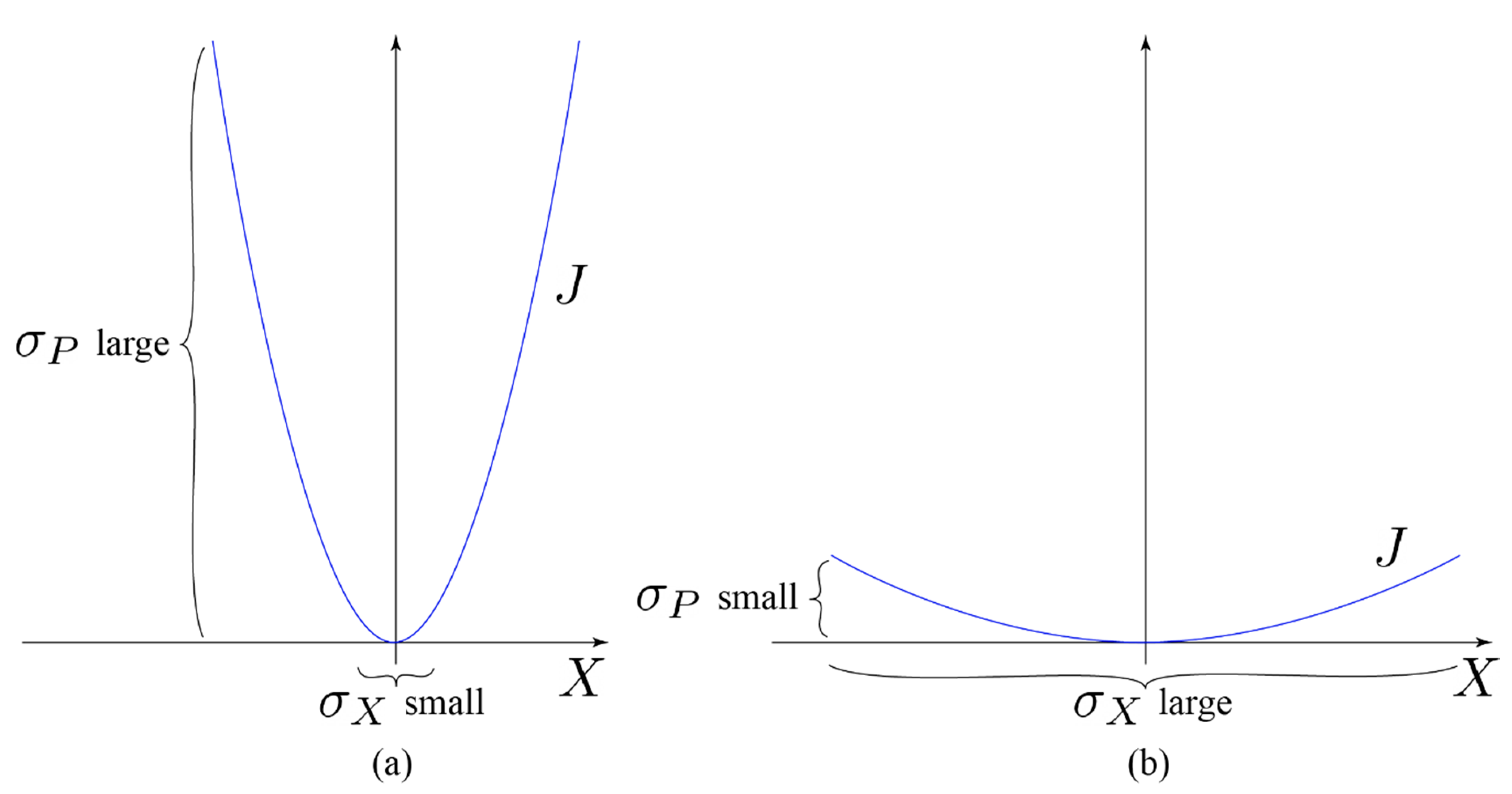
Intuitively, the content of the uncertainty principle is, in the present model, that the product of the standard deviations has a lower bound in terms of the stationary distribution due to the covariance. If one would like to have a small standard deviation for the position, one would need to have a rather steep value function in order to constrain and confine the particle within a small location in terms of the stationary distribution (due to the exponential structure of the Gibbs distribution). A steep and a localized value function $J$ would then imply a large standard deviation for the gradient of the value function. There is then a natural tradeoff between the localizations of four-position and four-momentum (Figure 1). The key is the gradient structure of the stochastic process, where the test particle tries to seek a minimum for the value function as in a “gradient search”.

Therefore, if one seeks an equilibrium system which has a very deep potential well and thus good localization and confinement properties, one needs to accept the large variability in the gradient of the potential (= value) function. This understanding of the uncertainty principle then implies that the lower bound for the product of standard deviations has nothing to do with experiments interfering with the set-up, but it is merely a natural trade-off implied by the linear–quadratic structure of the stochastic optimal control program. Indeed, one can see the framework through the lens of thermodynamics, where the system relaxes towards a thermodynamic equilibrium, which is just the stationary state for the respective Fokker–Planck equation. The results in this paper seem to therefore strongly support the statistical or the ensemble interpretation of quantum mechanics, put forward by, for example, Ballentine [6].

4. Conclusions

We believe that the Heisenberg uncertainty principle can be understood in a fruitful manner by considering it as a stationarity property of stochastic or statistical mechanics. The ontological and epistemological problems related to the uncertainty principle can be mitigated with such an interpretation as in the stochastic optimal control framework; the tradeoff of standard deviations between the four-position and the four-momentum can be understood intuitively through the confinement properties of the value function. The sharp localization, and thus small standard deviation of the test particle four-position, requires a rather steep value function locally, which naturally implies large variability for the gradient of the value function and thus for the four-momentum. Within this interpretation, it still holds that we cannot measure momentum and position simultaneously to an arbitrary degree of precision repetitively, but the uncertainty principle has a new, more intuitive meaning based on scientific realism and objectivism. The interpretation of the uncertainty principle, in which the measurement process itself causes the interference and the uncertainty limit, should be therefore finally abandoned.

The present model allows scientific realism and objectivism in the sense that the test particle obeys an optimal diffusion irrespective of the observer and its position and momentum are uniquely defined and measurable in principle at each point in spacetime, but as we repetitively measure something such as electrons from a beam, the fluctuations of the spacetime induce such randomness to the system that on average we can only “see” the ensemble in the “thermodynamic” equilibrium. In this sense, we argue that this study, together with [1], is very much a constructive model of an objective interpretation of quantum mechanics put forward by Karl Popper [5], among others. Moreover, the interpretation given in this article implies that the uncertainty principle does not logically rule out determinism as such. There is, however, a conceptual connection to Bohmian mechanics, due to the gradient drift structure and the quantum equilibrium, but as we have argued, the diffusion is a phenomenological model for the fluctuation of the spacetime itself. In a sense, the “hidden variables” are not needed, because the medium (spacetime) is stochastic. It is a modeling paradigm, from which one cannot, however, deduce whether the universe is deterministic or not. The optimization procedure, which nature seems to obey, just implies that certain random variables (due to the fluctuations of spacetime) must have a non-vanishing correlation. These conclusions are also in line with rather recent experimental evidence; see [10,11]. The present result seems to also support the paradigm that such uncertainty principles are general features of specific stochastic systems, as has been indicated, for example, in [4]. The symmetries of the present framework are manifested clearly in the property that the covariance of the four-position and the four-momentum is non-vanishing and invariant.

References

- Lindgren, J.; Liukkonen, J. Quantum mechanics can be understood through stochastic optimization on spacetimes. Sci. Rep. 2019, 9, 1–8. [Google Scholar] [CrossRef]
- Heisenberg, W. Über den anschaulichen inhalt der quantentheoretischen kinematik und mechanik. In Original Scientific Papers Wissenschaftliche Originalarbeiten; Springer: Berlin/Heidelberg, Germany, 1985; pp. 478–504. [Google Scholar]
- Ozawa, M. Physical content of Heisenberg’s uncertainty relation: Limitation and reformulation. Phys. Lett. A 2003, 318, 21–29. [Google Scholar] [CrossRef] [Green Version]
- Koide, T.; Kodama, T. Generalization of uncertainty relation for quantum and stochastic systems. Phys. Lett. A 2018, 382, 1472–1480. [Google Scholar] [CrossRef] [Green Version]
- Popper, K. Quantum Theory and the Schism in Physics; Psychology Press: Hove, UK, 1992. [Google Scholar]
- Ballentine, L.E. The statistical interpretation of quantum mechanics. Rev. Mod. Phys. 1970, 42, 358–381. [Google Scholar] [CrossRef]
- Bohm, D. A suggested interpretation of the quantum theory in terms of “hidden” variables. I. Phys. Rev. 1952, 85, 166. [Google Scholar] [CrossRef]
- Frederick, C. Stochastic space-time and quantum theory. Phys. Rev. D 1976, 13, 3183–3191. [Google Scholar] [CrossRef]
- Pavliotis, G.A. Stochastic Processes and Applications, Diffusion Processes, the Fokker-Planck and Langevin Equations; Springer: New York, NY, USA, 2014. [Google Scholar]
- Rozema, L.A.; Darabi, A.; Mahler, D.H.; Hayat, A.; Soudagar, Y.; Steinberg, A.M. Violation of Heisenberg’s measurement-disturbance relationship by weak measurements. Phys. Rev. Lett. 2012, 109, 100404. [Google Scholar] [CrossRef] [Green Version]
- Erhart, J.; Sponar, S.; Sulyok, G.; Badurek, G.; Ozawa, M.; Hasegawa, Y. Experimental demonstration of a universally valid error–disturbance uncertainty relation in spin measurements. Nat. Phys. 2012, 8, 185–189. [Google Scholar] [CrossRef] [Green Version]
Figure 1.
The tradeoff between the localizations of four-position and four-momentum: (a) position localized; (b) momentum localized.
© 2020 by the authors. Licensee MDPI, Basel, Switzerland. This article is an open access article distributed under the terms and conditions of the Creative Commons Attribution (CC BY) license (http://creativecommons.org/licenses/by/4.0/).
Share and Cite
MDPI and ACS Style
Lindgren, J.; Liukkonen, J. The Heisenberg Uncertainty Principle as an Endogenous Equilibrium Property of Stochastic Optimal Control Systems in Quantum Mechanics. Symmetry 2020, 12, 1533. https://doi.org/10.3390/sym12091533
AMA Style
Lindgren J, Liukkonen J. The Heisenberg Uncertainty Principle as an Endogenous Equilibrium Property of Stochastic Optimal Control Systems in Quantum Mechanics. Symmetry. 2020; 12(9):1533. https://doi.org/10.3390/sym12091533
Chicago/Turabian StyleLindgren, Jussi, and Jukka Liukkonen. 2020. "The Heisenberg Uncertainty Principle as an Endogenous Equilibrium Property of Stochastic Optimal Control Systems in Quantum Mechanics" Symmetry 12, no. 9: 1533. https://doi.org/10.3390/sym12091533
Note that from the first issue of 2016, this journal uses article numbers instead of page numbers. See further details here.