Oblique Stagnation Point Flow of Nanofluids over Stretching/Shrinking Sheet with Cattaneo–Christov Heat Flux Model: Existence of Dual Solution

Abstract

In the present work we consider a numerical solution for laminar, incompressible, and steady oblique stagnation point flow of $\mathrm{Cu}-\mathrm{water}$ nanofluid over a stretching/shrinking sheet with mass suction $S$. We make use of the Cattaneo–Christov heat flux model to develop the equation of energy and investigate the qualities of surface heat transfer. The governing flow and energy equations are modified into the ordinary differential equations by similarity method for reasonable change. The subsequent ordinary differential equations are illuminated numerically through the function bvp4c in MATLAB. The impact of different flow parameters for example thermal relaxation parameter, suction parameter, stretching/shrinking parameter, free stream parameter, and nanoparticles volume fraction on the skin friction coefficient, local Nusselt number, and streamlines are contemplated and exposed through graphs. It turns out that the lower branch solution for the skin friction coefficient becomes singular in shrinking area, although the upper branch solution is smooth in both stretching and shrinking domain. For oblique stagnation-point flow the streamlines pattern are not symmetric, and reversed phenomenon are detected close to the shrinking surface. Also, we observed that the free stream parameter changes the direction of the oncoming flow and controls the obliqueness of the flow. The existing work mostly includes heat and mass transfer as a mechanism for improving the heat transfer rate, which is the main objective of the authors.

1. Introduction

The heat transfer phenomenon in engineering and industrial system is one of the most vital problem in today’s year. Such phenomenon arises during the exchange of temperature difference within two medium or physical systems. The Interfacial thermal resistance is the measurement of an interfacial resistance to thermal flow, also known as Kapitza resistance or thermal boundary resistance. The Kapitza resistance varies from the contact resistance (not electrical contact resistance), since it presents being at atomically perfect interfaces. At solid–liquid interfaces thermal resistance performs a major role in heat transfer, and poor interface thermal resistance provides an opportunity to minimize heat casualty. The behaviors and performance of nanosized equipment rely powerfully on the way the systems consume heat. Additional knowledge of nanoscale heat transfer problems is significant for the thermoelectric, micro photonic industries and microelectronic from the nanosized thermal management, the system reliability and optimization. The efficient thermal conductivity of $\mathrm{Cu}$ is greatly affected due to the interfacial resistance. This field has not been much examined and just a couple of studies have been done to know the essential mechanism of this resistance [1,2]. In the earlier two centuries, Fourier’s law of heat transfer was used to analyze heat transfer attributes. The principle shortcoming of Fourier’s law is that it gives rise to a parabolic equation of energy, which characterizes that any preliminary turbulence is detected immediately through the entire system. To control this problem Maxwell–Cattaneos [3] extended the classical Fourier’s law by considering thermal relaxation time into it, that allows the transportation of heat through the propagation of thermal waves with confined speed. In this model, Christov [4] offered thermal relaxation time by means of Oldroyd’s upper-convicted derivative to obtain the material-invariant composition. Currently, different investigation has been made by a lot of researchers to use the Cattaneo–Christov heat flux model as an alternative of Fourier’s law of heat transfer. Tibullo and Zampoli [5] studied the originality and validity of the solution of incompressible fluids with the Cattaneo–Christov heat flux model. Mustafa [6] discussed the flow of Maxwell fluid with the Cattaneo–Christov heat flux model past a stretching sheet and showed that the thermal relaxation time has opposite effect on the thermal boundary layer thickness. The Magneto-Hydrodynamics viscoelastic flow with Cattaneo-Christov heat flux model of a radiative Maxwell fluid through stretched permeable surface was discovered by Shahid and colleagues [7]. They verified that growing the suction/injection parameter amazingly declines the horizontal components of velocity, although opposite actions are detected for the normal component in their study. The three-dimensional burgers fluid flow and heat transfer with the Cattaneo–Christov heat flux is deliberated numerically by Khan and Khan [8]. Several more beneficence in this direction with stimulating models has been reviewed by Ciarletta and Straughan [9], Liu [10], and Salahuddin [11].

Oblique stagnation-point flow emerges when fluid from any source obliquely impinges on a firm obstacle at an arbitrary angle of incidence. Such type of flow is mathematically obtained when shear component of flow along the wall is added to the orthogonal stagnation point flow. The two-dimensional steady flow of a Newtonian fluid in the direction of oblique stagnation-point has been addressed by several engineers and researchers starting from the Stuart [12] work in 1959. Subsequently, this problem was independently studied by Tamada [13] and Dorrepaal [14]. Reza and Gupta [15] generalized the Chiam [16] study of stagnation point flow toward a stretching surface with various wall stretching estimates from that of the stagnation flow by ignoring the pressure gradient and displacement thickness. The limited assistance toward this problem was given by Lok [17] in his paper. But he did not take pressure gradient in the far field boundary conditions. Drazin and Riley [18] further studied this problem together with free stream parameter added to the shear flow component associated with pressure gradient. Weidman and Putkaradze [19] investigated the axisymmetric flow on a circular cylinder toward oblique stagnation point by means of coupled ordinary differential equations. Considerable aspects of two dimensional steady and unsteady oblique and orthogonal stagnation flow toward a starching or shrinking surface has been evaluated by many researchers [20,21,22,23].

In recent times reasonable interest has been created in the study of stretching boundary because of its abundant and cumulative engineering and manufacturing applications including paper production, bundle wrapping, sheet extraction, hot rolling, cooling of electronic chips or metallic sheet, and many more. In sight of such circumstances the final compound of required features relies on the cooling rate and the technique of stretching. In the light of these useful implementation, huge efforts have been made in numerous directions for heat transfer and boundary layer flow through stretchable surface [24,25]. Sakiadis [26] was the first to describe the two-dimensional boundary layer flow over a stretching surface. Crane [27] further studied this idea and established a closed-form solution over a stretchable surface. After that the concept of stretching sheet have been developed by few scientists [28,29,30] for different models of fluid. In contrast, the study of shrinking sheet has drawn special attention of authors because of their captivating features. The problems of shrinking sheet are beneficial in observing the shrink-swell comportment, capillary effects in extremely diminutive openings, and the hydraulic characteristics of cultivated loam which are preeminent for agricultural enlargement and environmental administration policies. The leading work on the shrinking surface was adopted by Wang [31] in 1990. Later, Miklavcic and Wang [32] achieved an analytical result for hydrodynamic viscous flow through shrinking surface. In the presence of shrinking sheet, Wang [33] deliberated the flow of stagnation point. Using the Adomian decomposition method, Noor et al. [34] set up a series solution for magnetohydrodynamic viscous flow over a shrinking surface. Further studies on two and three-dimensional flow resulting from the shrinking sheet can be seen in references [35,36,37].

Recently the research on heat flux and heat transfer of nanofluid has gained extensive concentration because of excessive improvement in thermal conductivity of conventional fluids. Nanofluid technology has also extensive application in biomedical and processing system engineering including drug delivery, living organisms on their prime cellular level, phototherapy, fracture shrimps and super-hydrophobic beetle wings, usage of electric polymers for lubrication, molecular motors, chromatography, cancer therapeutics and diagnosis, in vivo therapy, neuro electronic interfaces, and protein engineering etc. Choi [38] developed the term nanofluid by appending the nano-sized particles in base fluids and declared that fluids with suspended nanoparticles consume high thermal conductivity. Masuda [39] also observed the refinement in the thermal conductivity of common fluid caused by the inclusion of nanoparticles. Wang [40] conducted a research on a viscous nanofluid through a stretching sheet in the presence of slip effect and mass suction. Buongiorno [41] presented a complete review of convective transportation in nanofluids while khan and Pop [42] applied the Buongiorno model [41] and observed the boundary layer flow of a nanofluid with existence of stretching sheet. Some remarkable surveys associated with the flow of nanofluid can be seen in references [43,44,45,46,47,48,49,50].

All of the above stated investigations related to the flow of stagnation point with a stretching/shrinking sheet in a viscous and Newtonian fluid. Nadeem et al. [20] investigated the MHD oblique stagnation point flow of nanofluid toward a stretching/shrinking sheet with existence of dual solutions. To the best knowledge of the authors no studies have previously reported the oblique stagnation flow of a nanofluid past a stretching/shrinking sheet with the Cattaneo–Christov heat flux model. Therefore, the prime objective of our study is to extend the work of Nadeem et al. [20] by taking heat transfer characteristics of the Cattaneo–Christov heat flux model. Numerical solutions for the governing flow and energy equations are gained using the effective bvp4c function in MATLAB. The behavior of skin friction coefficient and local Nusselt number are analyzed against various values of relevant parameters. The corresponding results are exposed graphically, and the successful features of the problem are deliberated.

2. Basic Equations

Consider an incompressible, two-dimensional, laminar and steady oblique stagnation point flow of $\mathrm{Cu}-\mathrm{water}$ nanofluid through stretching/shrinking sheet. We make use of the Cattaneo–Christov heat flux model to develop the energy equation. The cartesian coordinates $x$ and $y$ are taken along and normal to the sheet while $\left(u,v\right)$ are velocity components along $x$ and $y$ direction respectively. The surface velocities are assumed $u=ax$ and $v=-{\nu }_w$ where $a<0$ represents shrinking sheet, $a>0$ represents stretching sheet, ${\nu }_w>0$ refers to mass suction, and ${\nu }_w<0$ refers to mass injection.

It is recognized that the outer flow, in terms of ψ, is the partnership of basic shear flow and the orthogonal stagnation flow as [51]

$$\psi =a\left(\frac{\alpha }{2}{y}^2+xy-Ax-\alpha By+\alpha BA-\frac{\alpha }{2}{A}^2 \right) ,$$

(1)

Here $a$ represents the ability of an irrotational straining flow, $\alpha$ signifying the dimensionless constant that presents the ratio of the vorticity of a rotational shear flow to the strength of an irrotational straining flow, $A, B$ are constants to such an extent that $A$ is resolved as the major aspect of the solution of the orthogonal flow, and $B$ is a free parameter. Additionally, $B-A$ decides the displacement of the uniform shear flow parallel to the wall $y=0$. By characterizing $\psi$ in a regular way, $u=\frac{\partial \psi }{\partial y}$ and $v=-\frac{\partial \psi }{\partial x}$, the outer flow velocities are

$$u=a\left(x+\alpha \left(y-B\right)\right), v=-a\left(y-A\right).$$

(2)

Under these assumptions, the flow field equation becomes as [52]

$$\frac{\partial u}{\partial x}+\frac{\partial u}{\partial y}=0,$$

(3)

$$u\frac{\partial u}{\partial x}+v\frac{\partial u}{\partial y}=-\frac{1}{{\rho }_{nf}}\frac{\partial p}{\partial x}+\frac{{\mu }_{nf}}{{\rho }_{nf}}\left(\frac{{\partial }^{2}u}{\partial x^2}+\frac{{\partial }^{2}u}{\partial y^2}\right),$$

(4)

$$u\frac{\partial v}{\partial x}+v\frac{\partial v}{\partial y}=-\frac{1}{{\rho }_{nf}}\frac{\partial p}{\partial y}+\frac{{\mu }_{nf}}{{\rho }_{nf}}\left(\frac{{\partial }^{2}v}{\partial x^2}+\frac{{\partial }^{2}v}{\partial y^2}\right),$$

(5)

$${\left(\rho C_p\right)}_{nf}\left(u\frac{\partial T}{\partial x}+v\frac{\partial T}{\partial y}\right)=-\nabla \cdot q$$

(6)

where $q$ represents the heat flux and are defined for the Cattaneo–Christov heat flux model [1] as

$$q+\epsilon \left[V.\nabla q-q.\nabla V+\left(\nabla .V\right)q\right]=k_{nf}\nabla T$$

(7)

containing thermal relaxation time $\epsilon$ and $V=\left(u,v\right)$. In view of Equation (7) we can write Equation (6) as

$$u\frac{\partial T}{\partial x}+v\frac{\partial T}{\partial y}+\epsilon \left(u\frac{\partial u}{\partial x}\frac{\partial T}{\partial x}+u\frac{\partial v}{\partial x}\frac{\partial T}{\partial y}+v\frac{\partial u}{\partial y}\frac{\partial T}{\partial x}+v\frac{\partial v}{\partial y}\frac{\partial T}{\partial y}+u^2\frac{{\partial }^{2}T}{\partial x^2}+v^2\frac{{\partial }^{2}T}{\partial y^2}+2uv\frac{{\partial }^{2}T}{\partial x\partial y}\right)=\frac{k_{nf}}{{\left(\rho C_p\right)}_{nf}}\left(\frac{{\partial }^{2}T}{\partial x^2}+\frac{{\partial }^{2}T}{\partial y^2}\right)$$

(8)

The associated boundary constraints for flow equations are

$$\begin{array}{c}u=bx, v=-{\nu }_w=-\sqrt{a\frac{{\mu }_f}{{\rho }_f}}S, T=T_w at y=0\\ u=a\left(x+\alpha \left(y-B\right)\right), v=-a\left(y-A\right), T=T_{\infty }as y\to \infty \end{array}\}$$

(9)

where $S$ is a nondimensional constant which represents the strength of mass suction and ${\mu }_{nf},{\rho }_{nf}$, ${\left(\rho C_p\right)}_{nf}$ $k_{nf}$ are the dynamic viscosity, mass density, heat capacity, and thermal conductivity of the nanofluid respectively, and are defied as [20].

$$\frac{{\mu }_{nf}}{{\mu }_f}={\left(1-\phi \right)}^{-2.5}, \frac{{\rho }_{nf}}{{\rho }_f}=\left(1-\phi \right)+\phi \frac{{\rho }_s}{{\rho }_f}, \frac{{\left(\rho C_p\right)}_{nf}}{{\left(\rho C_p\right)}_f}=\left(1-\phi \right)+\phi \frac{{\left(\rho C_p\right)}_s}{{\left(\rho C_p\right)}_f},$$

$$\frac{k_{nf}}{k_f}=\frac{\left(\frac{k_s}{k_f}+2\right)-2\phi \left(1-\frac{k_s}{k_f}\right)}{\left(\frac{k_s}{k_f}+2\right)+\phi \left(1-\frac{k_s}{k_f}\right)}.$$

in which $\phi$ represent the nanoparticle volume fraction, ${\mu }_f$ is the dynamic viscosity of base fluid, ${\rho }_s$, ${\rho }_f$ are the mass density of nanoparticle and base fluid, respectively, ${\left(\rho C_p\right)}_s$, ${\left(\rho C_p\right)}_f$ are the heat capacity of nanoparticles and base fluid, respectively and $k_s$, $k_f$ represents the thermal conductivity of nanoparticle and base fluid, respectively, and the thermophysical values are given in

Table 1. Properties of fluid and nanoparticles [53].

Thermophysical Properties	Cu	Pure Water
$C_p\left(J/kgK\right)$	$385$	$4179$
$\rho \left(kg/m^3\right)$	$8933$	$997.1$
$k \left(W/mK\right)$	$401$	$0.613$

.

Using $p_{xy}=p_{yx}$ for eliminating the pressure field from Equations (4) and (5) and the similarity solutions as given in Equation (10)

$$u=ax{f}^{\prime }\left(\eta \right)+\sqrt{\frac{a{\mu }_f}{{\rho }_f}}g\left(\eta \right), v=-\sqrt{\frac{a{\mu }_f}{{\rho }_f}}f\left(\eta \right),\eta =\sqrt{\frac{a{\rho }_f}{{\mu }_f}}y,\theta \left(y\right)=\frac{T-T_{\infty }}{T_w-T_{\infty }}$$

(10)

Equations (3)–(9) reduces to

$$\frac{{\mu }_{nf}}{{\mu }_f}\frac{{\rho }_f}{{\rho }_{nf}}{f}^{iv}+f{f}^{‴}- f^{\prime } f^{’’}=0,$$

(11)

$$\frac{{\mu }_{nf}}{{\mu }_f}\frac{{\rho }_f}{{\rho }_{nf}}{g}^{‴}+f{g}^{″}-g{f}^{″}=0,$$

(12)

$$\frac{1}{Pr}\frac{k_{nf}}{k_f}{\theta }^{″}+\frac{{\left(\rho C_p\right)}_{nf}}{{\left(\rho C_p\right)}_f}f{\theta }^{\prime }-\gamma \frac{{\left(\rho C_p\right)}_{nf}}{{\left(\rho C_p\right)}_f}\left(f{f}^{\prime }{\theta }^{\prime }+f^2{\theta }^{″}\right)=0.$$

(13)

$$\begin{array}{c}f\left(0\right)=S, f^{\prime }\left(0\right)=\lambda , g\left(0\right)=0, \theta \left(0\right)=1,\\ f^{\prime }\left(\eta \right)=1, \theta \left(\eta \right)=0 as \eta \to \infty \\ f\left(\eta \right)=\eta -A, g\left(\eta \right)=\alpha \left(\eta -\mathbb{B}\right) as \eta \to \infty \end{array}\}$$

(14)

where $\gamma =\epsilon b$ is a thermal relaxation time, $\lambda =\frac{b}{a}$ represents stretching/shrinking parameter, $\mathbb{A}=\sqrt{\frac{a{\rho }_f}{{\mu }_f}}A$, $\mathbb{B}=\sqrt{\frac{a{\rho }_f}{{\mu }_f}}B$ are constant parameters, and $Pr=\frac{{\mu }_f}{{\rho }_f}\frac{{\left(\rho C_p\right)}_f}{k_f}$ is a Prandtl number.

Now integrating Equations (11) and (12) and using the extreme condition defined in (14), Equations (11) and (12) reduces to

$$\frac{{\mu }_{nf}}{{\mu }_f}\frac{{\rho }_f}{{\rho }_{nf}}{f}^{‴}+f{f}^{″}-{\left( f^{\prime }\right)}^2+1=0,$$

(15)

$$\frac{{\mu }_{nf}}{{\mu }_f}\frac{{\rho }_f}{{\rho }_{nf}}{g}^{″}+f{g}^{\prime }-g{f}^{\prime }-\alpha \left(B-A\right)=0,$$

(16)

For the streamlines, we find the non-dimensional stream function $\psi$ from Equation (17)

$$\frac{{\rho }_f}{{\mu }_f}\psi =\xi f\left(\eta \right)+\underset{0}{\overset{\eta }{{\displaystyle \int }}}g\left(s\right)ds$$

(17)

where $\xi =\sqrt{\frac{a{\rho }_f}{{\mu }_f}}x=\sqrt{\frac{a}{\upsilon }}x$. The point where $\psi /\upsilon = \frac{{\rho }_f}{{\mu }_f}\psi = 0$ meet the surface is denoted as ${\xi }_0$. Further, the dimensionless form of Equation (1), shows that the streamlines are hyperbolas whose asymptotes are

$$\eta =\mathbb{A}, \eta =-\frac{2}{\alpha }\xi +2\mathbb{B}-\mathbb{A},$$

(18)

These lines are also known as the degenerate streamlines or dividing streamlines.

From Equation (18) we can find the slope of dividing streamline as

$$slope=-\frac{2}{\alpha },$$

(19)

This line makes an angle $\vartheta$ with the plate as given in Equation (20) [51].

$$\vartheta ={\tan }^{-1}\left(-\frac{2}{\alpha }\right)$$

(20)

Equation (20) shows that the inclination angle varies, only, with respect to $\alpha$. Also, from Equations (17) and (18) we find that the stagnation point, ${\xi }_0$, occurs at the surface $\eta =\mathbb{A}$ rather than $\eta =0$.

The skin friction coefficient and local Nusselt number at the stretching/shrinking surface are given by [51].

$$C_f=\frac{{\tau }_w}{\frac{1}{2}{\rho }_f{U}_w^2}, Nu=\frac{x{q}_w}{k_f\left(T_w-T_{\infty }\right)}$$

(21)

where ${\tau }_w$ constitute the local wall shear stress and $q_{w }$ is the local heat flux and are determined as

$${\tau }_w={{\mu }_{nf}\frac{\partial u}{\partial y}|}_{y=0} \mathrm{and} q_w=-k_{nf}{\frac{\partial T}{\partial y}|}_{y=0}.$$

(22)

Making use of (10), system (21) and (22) reduces to

$$\begin{array}{c}\frac{1}{2}R{e}_x{C}_f=\frac{{\mu }_{nf}}{{\mu }_f}\left[\sqrt{Re}{f}^{″}\left(0\right)+g^{\prime }\left(0\right)\right],\\ {\left(R{e}_x\right)}^{-\frac{1}{2}}Nu=-\frac{k_{nf}}{k_f}{\theta }^{\prime }\left(0\right).\end{array}\}$$

(23)

In (23) $R{e}_x=\frac{{\rho }_f{U}_w^2}{a{\mu }_f}$ represents local Reynolds number. From ${\left(23\right)}_1$, we can easily find the point at the surface, ${\xi }_s,$ where the skin friction coefficient is zero, that is [51].

$${\xi }_s=-\frac{g^{\prime }\left(0\right)}{f^{″}\left(0\right)},$$

(24)

Equation (24) shows that the point ${\xi }_s$ depends on all the flow parameters but greatly depends on the stretching/shrinking parameter $\lambda$.

3. Results and Discussion

Using MATLAB function bvp4c the numerical solutions for the closing system of equations of ODEs with associated boundary conditions (13)–(16) have been obtained. For details of this method see Shampine et al. [54]. The outputs obtained through the bvp4c scheme are displayed graphically for multiple values of different parameters viz. suction parameter $\mathrm{S}$, stretching/shrinking parameter $\lambda$, thermal relaxation parameter $\mathsf{\gamma }$, free stream parameter $\mathsf{\alpha }$, and the nanoparticles volume fraction $\phi$. Results for $f^{″}\left(0\right),$ $g^{\prime }\left(0\right), -{\theta }^{\prime }\left(0\right),$ and ${\xi }_0$ are graphically presented with certain variations in the dimensionless parameters as shown in Figure 1, Figure 2 and Figure 3. Moreover, the pattern of streamlines along the shrinking surface for several values of free stream parameter $\alpha$ are displayed in Figure 4. Note that for $\alpha =0$ orthogonal streamlines are obtained. For the validation of the numerical method used, the results were compared with earlier studies.

Table 2. Values of $g_0^{\prime }\left(0\right)$ for some values of $\mathbb{B}-\mathbb{A}$ when $\lambda =\phi =M=S=\gamma =0$.

$\mathbb{A}$	${\mathit{f}}^{″}\left(0\right)$	$\mathbb{B}-\mathbb{A}$	${\mathit{g}}^{\prime }\left(0\right)$
			Borrelli et al. [55]	Nadeem et al. [20]	Present Results
0.6479	1.23295	−5.6479	7.5693	7.56948	7.56945
		−0.6479	1.4065	1.40655	1.40655
		0	0.6080	0.60796	0.60798
		0.6479	−0.1906	−0.19063	−0.19064
		4.3521	−4.7562	−4.75638	−4.75631

shows that the present results are in a very good agreement with the values obtained by Borrelli et al. [55] and Nadeem et al. [20]. Therefore, the validity and effectiveness of bvp4c method is proven.

The impact of $S$ on $f^{″}\left(0\right)$ $\mathrm{and}$ $g^{\prime }\left(0\right)$ both for stretching ($\lambda >0$) and shrinking ($\lambda <0$) surface have been respectively analyzed in Figure 1a,b. From these figures, we determine the critical values, ${\mathsf{\lambda }}_{\mathrm{c}}$, for stretching/shrinking parameter, $\lambda$, where we notice that there is no solution for $\lambda < {\lambda }_c$, unique solution exists for $\lambda = {\lambda }_c$ and dual solutions for $\lambda > {\lambda }_c$. The critical values ${\lambda }_c$ appear in the shrinking region $\lambda <0$, whereas the dual solution exists in both stretching and shrinking domain, whenever, $\lambda > {\lambda }_c$. Furthermore, from Figure 1a,b we can see that both $f^{″}\left(0\right)$ and $g^{\prime }\left(0\right)$ enhances for the first solution and declines for the second solution with enlarging values of mass suction $S.$ Figure 1c,d respectively shows the behavior of $-{\theta }^{\prime }\left(0\right)$ and ${\xi }_0$ with respect to stretching/shrinking parameter, $\mathsf{\lambda }$ for distinct values of mass suction $\mathrm{S}$. From these figures, we decided that with the increase of suction parameter $\mathrm{S}$, both $-{\theta }^{\prime }\left(0\right)$ and ${\xi }_0$ decreases whereas the higher values of shrinking parameter, $\lambda$ $(\lambda <0)$ enlarges both $-{\theta }^{\prime }\left(0\right)$ and ${\xi }_0$. Also, $\mathrm{S}$ increases the range of critical values for $\lambda$, i.e., ${\mathsf{\lambda }}_{\mathrm{c}}$ which means that mass suction increases the range of solution region. In Figure 2 again we have plotted $f^{″}\left(0\right)$, $g^{\prime }\left(0\right)$, $-{\theta }^{\prime }\left(0\right),\mathrm{and} {\xi }_0$ over a stretching/shrinking surface $\lambda$, for individual values of nanoparticles volume fraction, $\phi =0,0.1,0.2$. and fixed values of $\alpha =1, \gamma =0.01,S=3.0,\mathbb{B}=\mathbb{A}$ and $Pr=6.2$. From these plots, we found that $f^{″}\left(0\right)$ and $g^{\prime }\left(0\right)$ increases as nanoparticles volume fraction $\mathsf{\phi }$ increases. Moreover, increment of $\mathsf{\phi }$ supports the improvement of both $-{\theta }^{\prime }\left(0\right)\mathrm{and}{\xi }_0$. Also, $\mathsf{\phi }$ increases the range of critical values i.e., ${\lambda }_c$, which means that $\mathsf{\phi }$ increases the range of stretching/shrinking where solution exist.

The results presented in Figure 3 leads to the behavior of $-{\theta }^{\prime }\left(0\right)$ for different suction $\left(\mathrm{a}\right)$ $S=2$ and $\left(\mathrm{b}\right)$ $S=3$ against $\mathsf{\lambda }$ and several values of thermal relaxation parameter γ when $\alpha =1,\phi =0.2,\mathbb{B}=\mathbb{A}$ and $Pr=6.2.$ It is notified from Figure 3 that the outcomes of magnifying values of thermal relaxation parameter $\mathsf{\gamma }$ leads to decrease of $-{\theta }^{\prime }\left(0\right)$ and vice versa. Since we have one way coupling of momentum equation and temperature equation, therefore, thermal relaxation parameter γ, does not influence the skin friction coefficient, also it has no effect on the critical values of stretching/shrinking parameter, i.e., ${\lambda }_c$, as seen in Figure 3.

The behavior of streamlines pattern along the shrinking sheet for both first and second solution have been exposed in Figure 4. In these plots, we have discussed three different cases of free stream parameter ($\alpha =2,\alpha =0,\alpha =-2$) for the fixed values of $\phi =0.2,\gamma =0.01, S=0.5, \lambda =-1,\mathbb{B}=\mathbb{A}$ and $\mathrm{Pr}=6.2$. From the first two plots of streamlines it is clearly seen that for positive values of free stream parameter, $\alpha$, oblique pattern of streamlines is obtained for both first and second solution and the dividing stream line strike the surface at the left side of the origin. This led us to say that for positive values of free stream parameter, i.e., $\alpha >0$, the stagnation point appears at $\xi <0$. For $\alpha =0$ the streamlines become identical to that of orthogonal stagnation flow and the stagnation point lies on the origin as show in plots $\left(\mathrm{c}\right)$ and $\left(\mathrm{d}\right)$ of Figure 4. Furthermore, for $\alpha =-2$, again the streamlines pattern becomes oblique and the dividing streamline strike the surface at the positive side, from the origin, as seen in the last two plots of the streamlines. This led us to say that for negative values of free stream parameter, i.e., $\alpha <0$, the stagnation point appears at $\xi >0$. These observations indicate that by increasing both positive and negative values of $\mathsf{\alpha }$ the obliquity of flow increases more and more. However, for $\alpha =0$ the flow field becomes orthogonal. The streamlines of second solutions demonstrates clearly that flow field is parted into two sub-regions one where flow is like a normal stagnation point flow and other presenting the reverse flow field.

4. Conclusions

The present work provides analysis of a steady two-dimensional viscous flow of a nanofluid over a stretching/shrinking sheet near the oblique stagnation point flow in the presence of mass suction. Cattaneo–Christov heat flux model has been utilized to explore the properties of surface heat transfer. The main outcomes of the present article are summarized as follows:

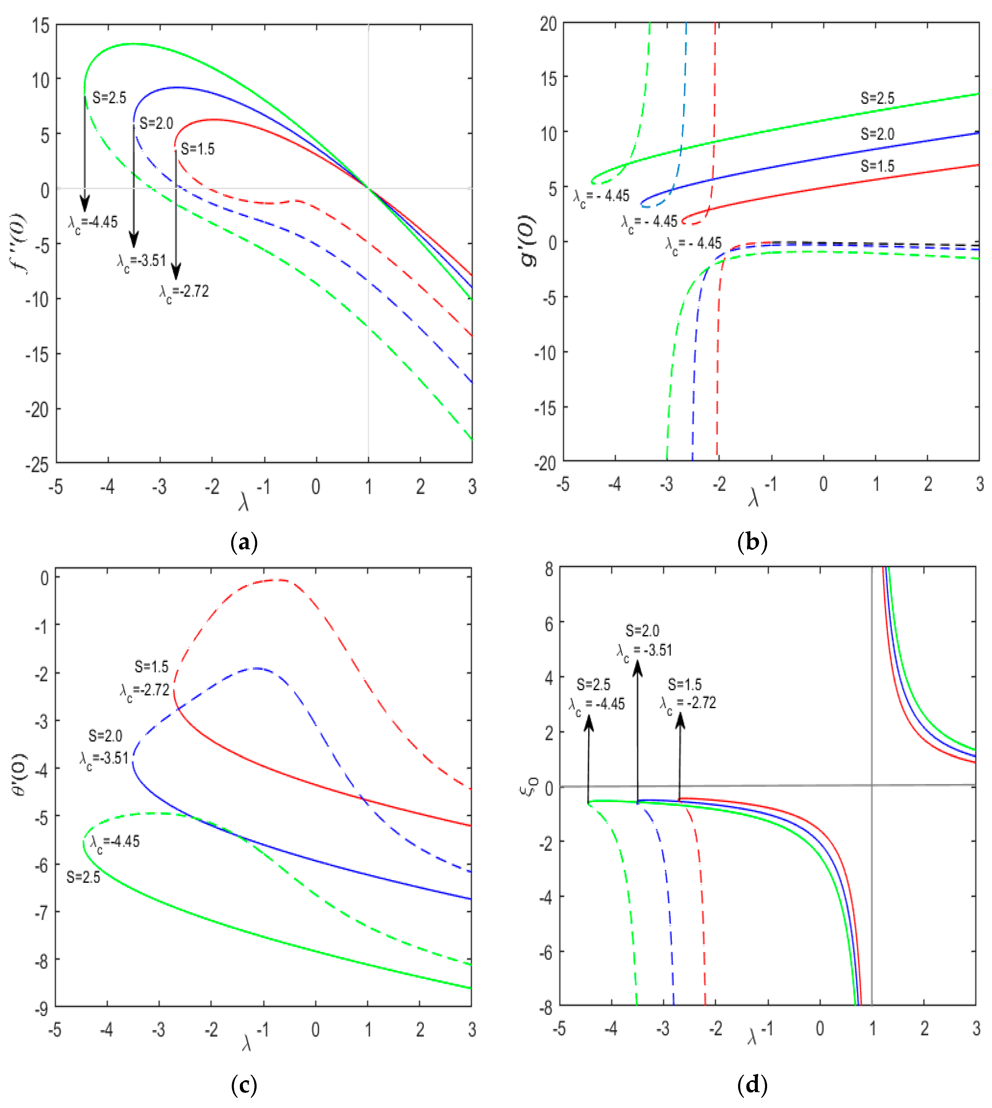
• Increasing the values of suction parameter $S$ gradually decreases the rate of heat transfer in a fluid both for first and second solutions. This rate is maximum when the sheet is shrunken and minimum when sheet is stretched.
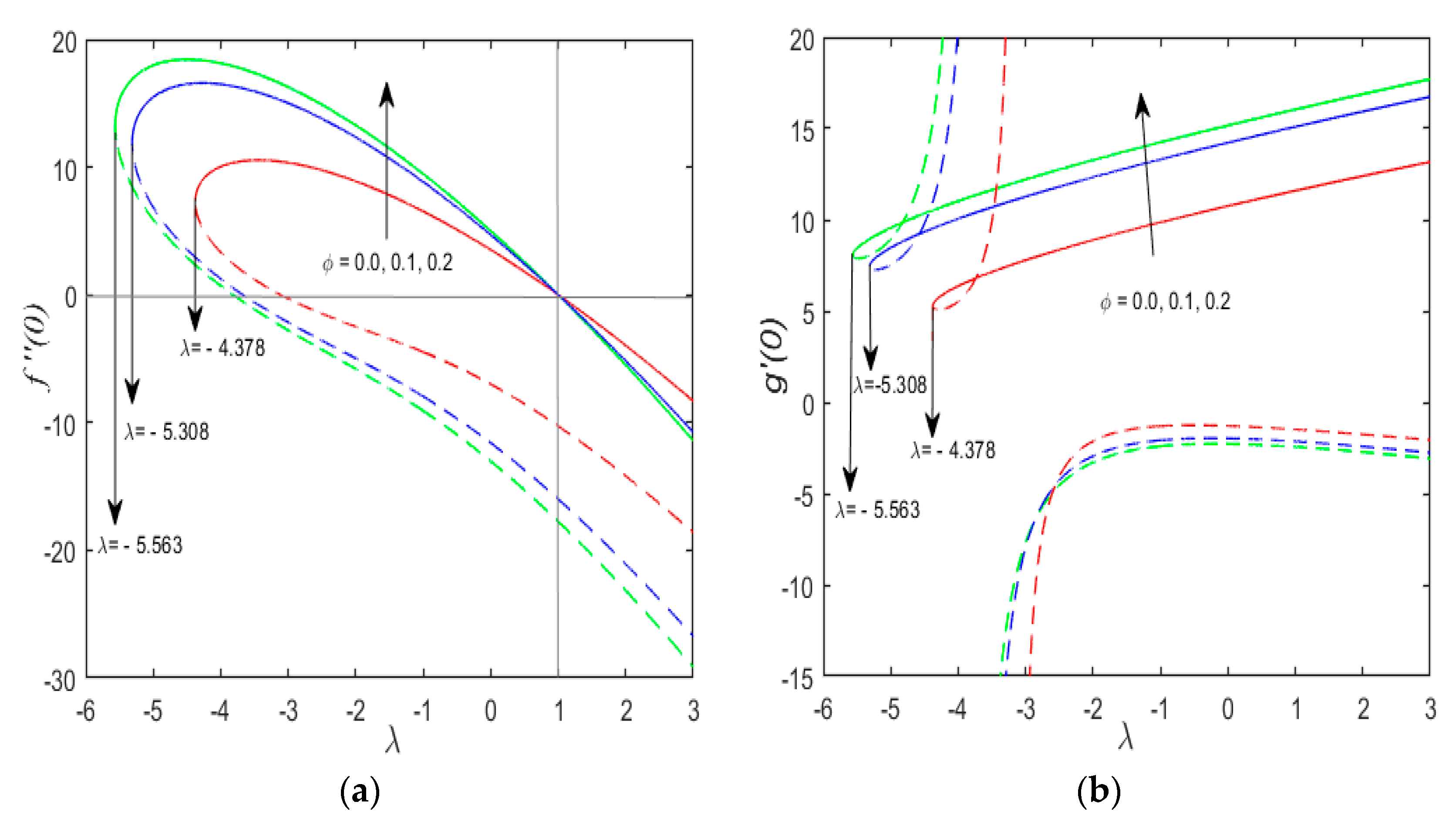
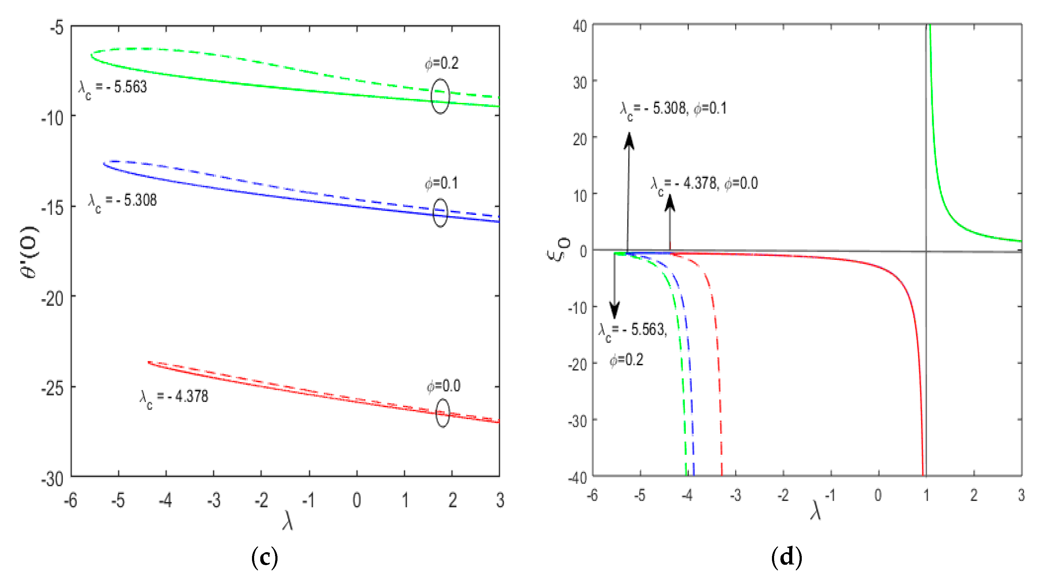
• Increasing the concentration of nanoparticles $\phi$ increases the rate of heat transfer in a fluid. Here $\phi$ has same effect both on first and second solution and $-{\theta }^{\prime }\left(0\right)$ is maximum for shrinking sheet as compared to stretching sheet.
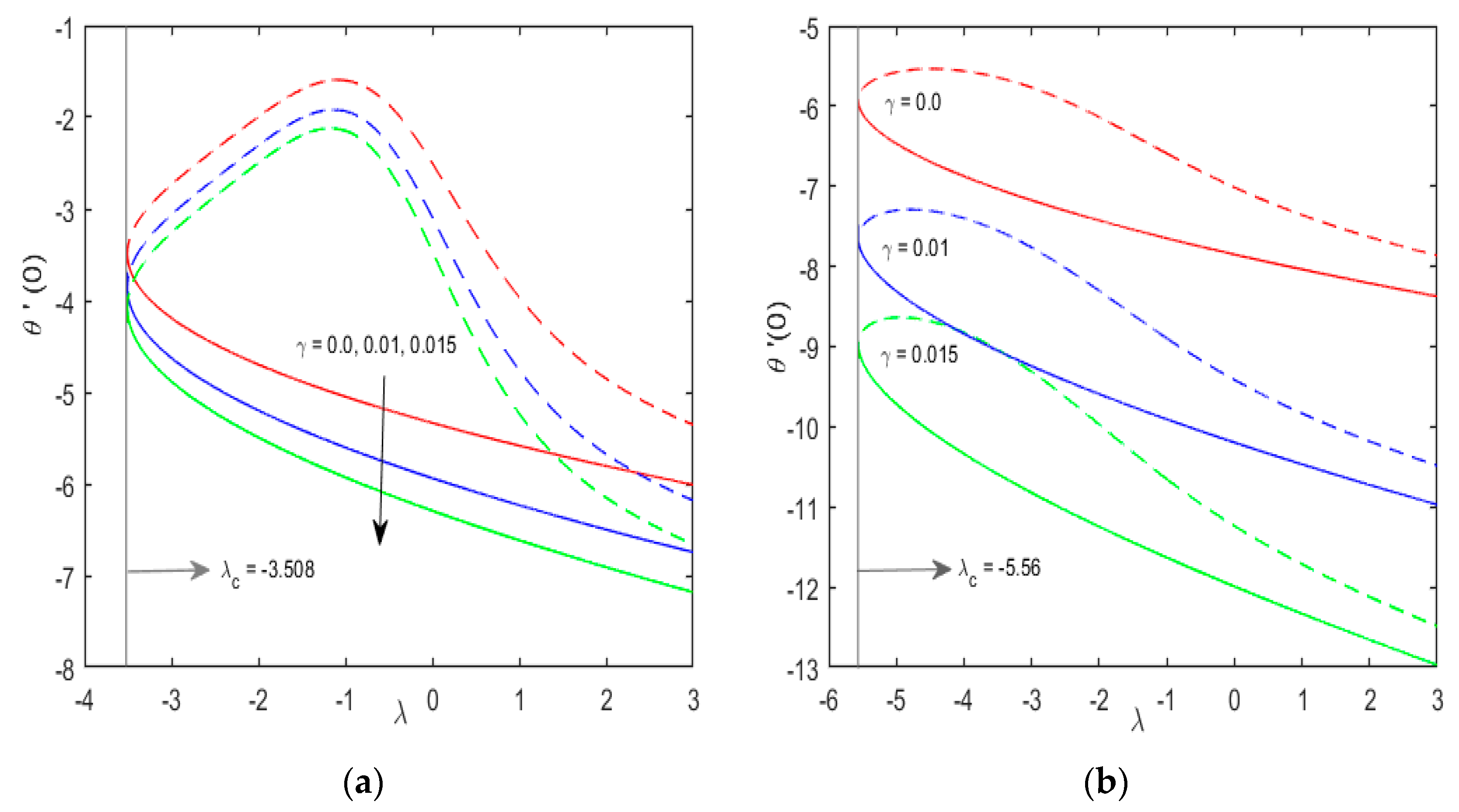
• It is notified that magnifying values of thermal relaxation parameter $\gamma$, only leads to a decrease in the rate of heat transfer $-{\theta }^{\prime }\left(0\right)$ and vice versa. Since we have one way coupling of momentum equation and temperature equation, therefore, thermal relaxation parameter γ, does not influence the skin friction coefficient, also it has no effect on the critical values of stretching/shrinking parameter, i.e., ${\lambda }_c$.
• The increasing values of $S$ and $\phi$ leads to an increase of $f^{″}\left(0\right)$.
• The local Nusselt number decreases with positive values of $\lambda$ (stretching sheet), however it increases with the negative values of $\lambda$ (shrinking sheet).
• ${\xi }_0$ decreases with high values of mass suction $S$.
• The streamlines pattern for three different values of free stream parameter $\alpha$ over a shrinking surface $\left(\lambda <0\right)$ shows that both positive and negative values of $\alpha$ increases the obliquity of flow toward the left or right of the origin, but for $\alpha =0$ orthogonal stagnation flow has been realized.

References

1. Vo, T.Q.; Kim, B. Transport Phenomena of Water in Molecular Fluidic Channels. Sci. Rep. 2016, 6, 33881. [Google Scholar]
2. Ge, Z.; Cahill, D.G.; Braun, P.V. Thermal conductance of hydrophilic and hydrophobic interfaces. Phys. Rev. Lett. 2006, 96, 186101. [Google Scholar] [CrossRef] [PubMed]
3. Cattaneo, C. Sulla conduzione del calore. Atti Sem. Mat. Fis. Univ. Modena. 1948, 3, 83–101. [Google Scholar]
4. Christov, C.I. On frame indifferent formulation of the Maxwell–Cattaneo model of finite-speed heat conduction. Mech. Res. Commun. 2009, 36, 481–486. [Google Scholar] [CrossRef]
5. Tibullo, V.; Zampoli, V. A uniqueness result for the Cattaneo–Christov heat conduction model applied to incompressible fluids. Mech. Res. Commun. 2011, 38, 77–79. [Google Scholar] [CrossRef]
6. Mustafa, M. Cattaneo-Christov heat flux model for rotating flow and heat transfer of upper-convected Maxwell fluid. AIP Adv. 2015, 5, 047109. [Google Scholar] [CrossRef]
7. Shahid, A.; Bhatti, M.M.; Bég, O.A.; Kadir, A. Numerical study of radiative Maxwell viscoelastic magnetized flow from a stretching permeable sheet with the Cattaneo–Christov heat flux model. Neural Comput. Appl. 2018, 30, 3467–3478. [Google Scholar] [CrossRef]
8. Khan, M.; Khan, W.A. Three-dimensional flow and heat transfer to burgers fluid using Cattaneo-Christov heat flux model. J. Mol. Liq. 2016, 221, 651–657. [Google Scholar] [CrossRef]
9. Ciarletta, M.; Straughan, B. Uniqueness and structural stability for the Cattaneo–Christov equations. Mech. Res. Commun. 2010, 37, 445–447. [Google Scholar] [CrossRef]
10. Liu, L.; Zheng, L.; Zhang, X. Fractional anomalous diffusion with Cattaneo–Christov flux effects in a comb-like structure. Appl. Math. Model. 2016, 40, 6663–6675. [Google Scholar] [CrossRef]
11. Salahuddin, T.; Malik, M.Y.; Hussain, A.; Bilal, S.; Awais, M. MHD flow of Cattanneo–Christov heat flux model for Williamson fluid over a stretching sheet with variable thickness: Using numerical approach. J. Magn. Magn. Mater. 2016, 401, 991–997. [Google Scholar] [CrossRef]
12. Stuart, J.T. The Viscous Flow Near a Stagnation Point When the External Flow Has Uniform Vorticity. J. Aerosp. Sci. 1959, 26, 124–125. [Google Scholar] [CrossRef]
13. Tamada, K. Two-Dimensional Stagnation-Point Flow Impinging Obliquely on a Plane Wall. J. Phys. Soc. Jpn. 1979, 46, 310–311. [Google Scholar] [CrossRef]
14. Dorrepaal, J.M. An exact solution of the Navier-Stokes equation which describes non-orthogonal stagnation-point flow in two dimensions. J. Fluid Mech. 1986, 163, 141. [Google Scholar] [CrossRef]
15. Reza, M.; Gupta, A.S. Steady two-dimensional oblique stagnation-point flow towards a stretching surface. Fluid Dyn. Res. 2005, 37, 334–340. [Google Scholar] [CrossRef]
16. Chaim, T.C. Stagnation-point flow towards a stretching plate. J. Phys. Soc. Jpn. 1994, 63, 2443–2444. [Google Scholar] [CrossRef]
17. Lok, Y.Y.; Amin, N.; Pop, I. Non-orthogonal stagnation point flow towards a stretching sheet. Int. J. Non-Linear Mech. 2006, 41, 622–627. [Google Scholar] [CrossRef]
18. Drazin, P.G.; Riley, N. The Navier-Stokes Equations: A Classification of Flows and Exact Solutions; Cambridge University Press: New York, NY, USA, 2006. [Google Scholar]
19. Weidman, P.D.; Putkaradze, V. Axisymmetric stagnation flow obliquely impinging on a circular cylinder. Eur. J. Mech. B/Fluids 2003, 22, 123–131. [Google Scholar] [CrossRef]
20. Nadeem, S.; Khan, M.R.; Khan, A.U. MHD oblique stagnation point flow of nanofluid over an oscillatory stretching/shrinking sheet: Existence of dual solutions. Phys. Scr. 2019, 94, 7. [Google Scholar] [CrossRef]
21. Ariel, P.D. Hiemenz flow in hydromagnetics. Acta Mech. 1994, 103, 31–43. [Google Scholar] [CrossRef]
22. Xu, H.; Liao, S.-J.; Pop, I. Series solutions of unsteady three-dimensional MHD flow and heat transfer in the boundary layer over an impulsively stretching plate. Eur. J. Mech. B/Fluids 2007, 26, 15–27. [Google Scholar] [CrossRef]
23. Gupta, P.S.; Gupta, A.S. Heat and mass transfer on a stretching sheet with suction or blowing. Can. J. Chem. Eng. 1977, 55, 744–746. [Google Scholar] [CrossRef]
24. Carragher, P.; Crane, L.J. Heat Transfer on a Continuous Stretching Sheet. ZAMM Zeitschrift für Angewandte Mathematik und Mechanik 1982, 62, 564–565. [Google Scholar] [CrossRef]
25. Dutta, B.K.; Roy, P.; Gupta, A.S. Temperature field in flow over a stretching sheet with uniform heat flux. Int. Commun. Heat Mass Transf. 1985, 12, 89–94. [Google Scholar] [CrossRef]
26. Sakiadis, B.C. Boundary-layer behavior on continuous solid surfaces: II. The boundary layer on a continuous flat surface. AIChE J. 1961, 7, 221–225. [Google Scholar] [CrossRef]
27. Crane, L.J. Flow past a stretching plate. Zeitschrift für Angewandte Mathematik und Physik ZAMP 1970, 21, 645–647. [Google Scholar] [CrossRef]
28. Ellahi, R.; Riaz, A. Analytical solutions for MHD flow in a third-grade fluid with variable viscosity. Math. Comput. Model. 2010, 52, 1783–1793. [Google Scholar] [CrossRef]
29. Nadeem, S.; Haq, R.U.; Akbar, N.S.; Lee, C.; Khan, Z.H. Numerical study of boundary layer flow and heat transfer of Oldroyd-B nanofluid towards a stretching sheet. PLoS ONE 2013, 8, e69811. [Google Scholar] [CrossRef]
30. Akbar, N.S.; Nadeem, S.; Haq, R.U.; Khan, Z.H. Numerical solutions of Magnetohydrodynamic boundary layer flow of tangent hyperbolic fluid towards a stretching sheet. Indian J. Phys. 2013, 87, 1121–1124. [Google Scholar] [CrossRef]
31. Wang, Y.C. Liquid film on an unsteady stretching surface. Q. Appl. Math. 1990, 48, 601–610. [Google Scholar] [CrossRef] [Green Version]
32. Miklavčič, M.; Wang, C. Viscous flow due to a shrinking sheet. Q. Appl. Math. 2006, 64, 283–290. [Google Scholar] [CrossRef] [Green Version]
33. Wang, C.Y. Stagnation flow towards a shrinking sheet. Int. J. Non. Linear. Mech. 2008, 43, 377–382. [Google Scholar] [CrossRef]
34. Noor, N.F.M.; Kechil, S.A.; Hashim, I. Simple non-perturbative solution for MHD viscous flow due to a shrinking sheet. Commun. Nonlinear Sci. Numer. Simul. 2010, 15, 144–148. [Google Scholar] [CrossRef]
35. Fang, T.; Zhang, J. Thermal boundary layers over a shrinking sheet: An analytical solution. Acta Mech. 2010, 209, 325–343. [Google Scholar] [CrossRef]
36. Midya, C. Hydromagnetic boundary layer flow and heat transfer over a linearly shrinking permeable surface. Int. J. Appl. Math. Mech. 2012, 8, 57–68. [Google Scholar]
37. Muhaimin; Kandasamy, R.; Hashim, I. Effect of chemical reaction, heat and mass transfer on nonlinear boundary layer past a porous shrinking sheet in the presence of suction. Nucl. Eng. Des. 2010, 240, 933–939. [Google Scholar] [CrossRef]
38. Choi, S.U.S.; Eastman, J.A. Enhancing Thermal Conductivity of Fluids with Nanoparticles; Argonne National Lab: Lemont, IL, USA, 1995. [Google Scholar]
39. Masuda, H.; Ebata, A.; Teramae, K. Alteration of thermal conductivity and viscosity of liquid by dispersing ultra-fine particles. Netsu Bussei 1993, 7, 227–233. [Google Scholar] [CrossRef]
40. Wang, C.Y. Analysis of viscous flow due to a stretching sheet with surface slip and suction. Nonlinear Anal. Real World Appl. 2009, 10, 375–380. [Google Scholar] [CrossRef]
41. Buongiorno, J. Convective transport in nanofluids. J. Heat Transfer. 2006, 128, 240–250. [Google Scholar] [CrossRef]
42. Khan, W.A.; Pop, I. Boundary-layer flow of a nanofluid past a stretching sheet. Int. J. Heat Mass Transf. 2010, 53, 2477–2483. [Google Scholar] [CrossRef]
43. Kakaç, S.; Pramuanjaroenkij, A. Review of convective heat transfer enhancement with nanofluids. Int. J. Heat Mass Transf. 2009, 52, 3187–3196. [Google Scholar] [CrossRef]
44. Hassani, M.; Tabar, M.M.; Nemati, H.; Domairry, G.; Noori, F. An analytical solution for boundary layer flow of a nanofluid past a stretching sheet. Int. J. Therm. Sci. 2011, 50, 2256–2263. [Google Scholar] [CrossRef]
45. Akyildiz, F.T.; Bellout, H.; Vajravelu, K.; van Gorder, R.A. Existence results for third order nonlinear boundary value problems arising in nano boundary layer fluid flows over stretching surfaces. Nonlinear Anal. Real World Appl. 2011, 12, 2919–2930. [Google Scholar] [CrossRef]
46. Dogonchi, A.S.; Ganji, D.D. Effect of Cattaneo–Christov heat flux on buoyancy MHD nanofluid flow and heat transfer over a stretching sheet in the presence of Joule heating and thermal radiation impacts. Indian, J. Phys. 2018, 92, 757–766. [Google Scholar] [CrossRef]
47. Kefayati, G.H.R.; Sidik, N.A.C. Simulation of natural convection and entropy generation of non-Newtonian nanofluid in an inclined cavity using Buongiorno’s mathematical model (Part II, entropy generation). Powder Technol. 2017, 305, 679–703. [Google Scholar] [CrossRef]
48. Kefayati, G.H.R. Simulation of natural convection and entropy generation of non-Newtonian nanofluid in a porous cavity using Buongiorno’s mathematical model. Int. J. Heat Mass Transf. 2017, 112, 709–744. [Google Scholar] [CrossRef]
49. Kefayati, G.H.R. Mixed convection of non-Newtonian nanofluid in an enclosure using Buongiorno’s mathematical model. Int. J. Heat Mass Transf. 2017, 108, 1481–1500. [Google Scholar] [CrossRef]
50. Kefayati, G.H.R. Lattice Boltzmann simulation of natural convection in a nanofluid-filled inclined square cavity at presence of magnetic field. Sci. Iran. Trans. B. Mech. Eng. 2013, 20, 1517. [Google Scholar]
51. Borrelli, A.; Giantesio, G.; Patria, M.C. MHD oblique stagnation-point flow of a micropolar fluid. Appl. Math. Model. 2012, 36, 3949–3970. [Google Scholar] [CrossRef]
52. Akbar, N.S.; Tripathi, D.; Khan, Z.H. Numerical investigation of Cattanneo-Christov heat flux in CNT suspended nanofluid flow over a stretching porous surface with suction and injection. Discret. Contin. Dyn. Syst. 2018, 11, 583–594. [Google Scholar] [CrossRef]
53. Nadeem, S.; Haq, R.U.; Khan, Z.H. Heat transfer analysis of water-based nanofluid over an exponentially stretching sheet. Alex. Eng. J. 2014, 53, 219–224. [Google Scholar] [CrossRef]
54. Shampine, L.F.; Kierzenka, J.; Reichelt, M.W. Solving boundary value problems for ordinary differential equations in MATLAB with bvp4c. Tutor. Notes 2000, 2000, 1–27. [Google Scholar]
55. Borrelli, A.; Giantesio, G.; Patria, M.C. MHD oblique stagnation-point flow of a Newtonian fluid. Zeitschrift für Angewandte Mathematik und Physik 2012, 63, 271–294. [Google Scholar] [CrossRef]
Figure 1. Behavior of physical quantities against λ and various values of S when α = 1 ,   γ = 0.01 ,   φ = 0.1 , B = A , and P r = 6.2 ; (a)   f ( 0 ) (b)   g ( 0 ) (c)   θ ( 0 ) (d)   ξ 0 .
Symmetry 11 01070 g001
Figure 2. Behavior of physical quantities against λ and different values of φ when α = 1 ,   γ = 0.01 ,   S = 3.0 , B = A , and P r = 6.2 ; (a)   f ( 0 ) (b)   g ( 0 ) (c)   θ ( 0 ) (d)   ξ 0 .
Symmetry 11 01070 g002aSymmetry 11 01070 g002b
Figure 3. Behavior of θ ( 0 ) against λ and different values of γ when α = 1 , φ   = 0.2 ,   B = A ,   and   P r = 6.2 .   ( a )   S = 2.0 ,   ( b )   S = 3.0 .
Symmetry 11 01070 g003
Figure 4. Streamlines pattern for both upper and lower solution branch for three different values of α when φ = 0.2 , γ = 0.01 , S = 0.5 , λ = 1 ,   B = A , P r = 6.2 ; (a)Upper branch solution for α = 2 (b) Lower branch solution for α = 2 (c) Upper branch solution for α = 0 (d) Lower branch solution for α = 0 (e) Upper branch solution for α = 2 (f) Lower branch solution for α = 2 .
Symmetry 11 01070 g004