Multi-Granulation Graded Rough Intuitionistic Fuzzy Sets Models Based on Dominance Relation

Abstract

From the perspective of the degrees of classification error, we proposed graded rough intuitionistic fuzzy sets as the extension of classic rough intuitionistic fuzzy sets. Firstly, combining dominance relation of graded rough sets with dominance relation in intuitionistic fuzzy ordered information systems, we designed type-I dominance relation and type-II dominance relation. Type-I dominance relation reduces the errors caused by single theory and improves the precision of ordering. Type-II dominance relation decreases the limitation of ordering by single theory. After that, we proposed graded rough intuitionistic fuzzy sets based on type-I dominance relation and type-II dominance relation. Furthermore, from the viewpoint of multi-granulation, we further established multi-granulation graded rough intuitionistic fuzzy sets models based on type-I dominance relation and type-II dominance relation. Meanwhile, some properties of these models were discussed. Finally, the validity of these models was verified by an algorithm and some relative examples.

1. Introduction

Pawlak proposed a rough set model in 1982, which is a significant method in dealing with uncertain, incomplete, and inaccurate information [1]. Its key strategy is to consider the lower and upper approximations based on precise classification.

As a tool, the classic rough set is based on precise classification. It is too restrictive for some problems in the real world. Considering this defect of classic rough sets, Yao proposed the graded rough sets (GRS) model [2]. Then researchers paid more attention to it and relative literatures began to accumulate on its theory and application. GRS can be defined as the lower approximation being ${\underset{\_}{R}}_k(X)=\{x||{[x]}_R|-|{[x]}_R\cap X|\le k,x\in U\}$ and the upper approximation being ${\overline{R}}_k(X)=\{x||{[x]}_R\cap X|>$ $k,x\in U\}.|{[x]}_R\cap X|$ is the absolute number of the elements of $|{[x]}_R|$ inside X and should be called internal grade, $|{[x]}_R|-|{[x]}_R\cap X|$ is the absolute number of the elements of $|{[x]}_R|$ outside X and should be called external grade. ${\overline{R}}_k(X)$ means union of the elements whose equivalence class’ internal-grade about X is greater than k, ${\underset{\_}{R}}_k(X)$ means union of the elements whose equivalence class’ external grade about X is at most k [3].

In the view of granular computing [4], the classic rough set is a single-granulation rough set. However, in the real world, we need multiple granularities to analyze and solve problems and Qian et al. proposed multi-granulation rough sets solving this issue [5]. Subsequently, multi-granulation rough sets were extended in References [6,7,8,9]. In addition, in the viewpoint of the degrees of classification error, Hu et al. and Wang et al. established a novel model of multi-granulation graded covering rough sets [10,11]. Simultaneously, Wu et al. constructed graded multi-granulation rough sets [12]. References [13,14,15,16,17] discussed GRS in a multi-granulation environment. Moreover, for GRS, it has been studied that the equivalence relation has been extended to the dominance relation [13,14], the limited tolerance relation [17] and so forth [10,11]. In general, all these aforementioned studies have naturally contributed to the development of GRS.

Inspired by the research reported in References [5,13,14,15,16,17], intuitionistic fuzzy sets (IFS) are also a theory which describe uncertainty [18]. IFS consisting of a membership function and a non-membership function are commonly encountered in uncertainty, imprecision, and vagueness [18]. The notion of IFS, proposed by Atanassov, was initially developed in the framework of fuzzy sets [19]. Furthermore, it can describe the “fuzzy concept” of “not this and not that”, that is to say, neutral state or neutral degree, thus it is more precise to portray the ambiguous nature of the objective world. IFS theory is applicable in decision-making, logical planning, medical diagnosis, machine learning, and market forecasting, etc. Applications of IFS have attracted people’s attention and achieved fruitful results [20,21,22,23,24,25,26,27].

In recent years, IFS have been a hot research topic in uncertain information systems [6,28,29,30]. For example, in the development of IFS theory, Ai et al. proposed intuitionistic fuzzy line integrals and gave their concrete values in Reference [31]. Zhang et al. researched the fuzzy logic algebraic system and neutrosophic sets as generalizations of IFS in References [23,26,27]. Furthermore, Guo et al. provided the dominance relation of intuitionistic fuzzy information systems [30].

Both rough sets and IFS not only describe uncertain information but also have strong complementarity in practical problems. As such many researchers have studied the combination of rough sets and IFS, namely, rough intuitionistic fuzzy sets (RIFS) and intuitionistic fuzzy rough sets (IFRS) [32]. For example, Huang et al., Gong et al., Zhang et al., He et al., and Tiwari et al. effectively developed IFRS respectively from uncertainty measures, variable precision rough sets, dominance–based rough sets, interval-valued IFS, and attribute selection [29,30,33,34,35]. Additionally, Zhang and Chen, Zhang and Yang, Huang et al. studied dominance relation of IFRS [19,20,21]. With respect to RIFS, Xue et al. provided a multi-granulation covering the RIFS model [9].

The above models did not consider the classification of some degrees of error [6,7,8,9,29,30,33,36] in dominance relation on GRS and dominance relation in intuitionistic fuzzy ordered information systems [37]. Therefore, in this paper, firstly, we introduce GRS into RIFS to get graded rough intuitionistic fuzzy sets (GRIFS) solving this problem. Then, considering the need for more precise sequence information in the real world, based on dominance relation of GRS and an intuitionistic fuzzy ordered information system, we respectively perform logical conjunction and disjunction operation to gain type-I dominance relation and type-II dominance relation. After that, we use type-I dominance relation and type-II dominance relation thereby replacing equivalence relation to generalize GRIFS. We design two novel models of GRIFS based on type-I dominance relation and type-II dominance relation. In addition, to accommodate a complex environment, we further extend GRIFS models based on type-I dominance relation and type-II dominance relation, respectively, to multi-granulation GRIFS models based on type-I dominance relation and type-II dominance relation. These models present a new path to extract more flexible and accurate information.

The rest of this paper is organized as follows. In Section 2, some basic concepts of IFS and GRS, RIFS are briefly reviewed, at the same time, we give the definition of GRS based on dominance relation. In Section 3, we respectively propose two novel models of GRIFS models based on type-I dominance relation and type-II dominance relation and verify the validity of these two models. In Section 4, the basic concepts of multi-granulation RIFS are given. Then, we propose multi-granulation GRIFS models based on type-I dominance relation and type-II dominance relation, and provide the concepts of optimistic and pessimistic multi-granulation GRIFS models based on type-I dominance relation and type-II dominance relation, respectively. In Section 5, we use an algorithm and example to study and illustrate the multi-granulation GRIFS models based on type-I dominance relation and type-II dominance relation, respectively. In Section 6, we conclude the paper and illuminate on future research.

2. Preliminaries

Definition 1

([22]). Let U be a non-empty classic universe of discourse. U is denoted by:

$$A=\{<x,{\mu }_A(x),{\nu }_A(x)>|x\in U\},$$

A can be viewed as IFS on U, where${\mu }_A(x):U\to [0,1]$and${\nu }_A(x):U\to [0,1]$.${\mu }_A(x)$and${\nu }_A(x)$are denoted as membership and non-membership degrees of the element$x$in A, satisfying$0\le {\mu }_A(x)+{\nu }_A(x)\le 1$. For$\forall x\in U$, the hesitancy degree is${\pi }_A(x)=1-{\mu }_A(x)-{\nu }_A(x)$, noticeably,${\pi }_A(x):U\to [0,1]$.$\forall A,B\in$$IFS(U)$, the basic operations of A and B are given as follows:

$(1)A\subseteq B\iff {\mu }_A(x)\le {\mu }_B(x),{\nu }_A(x)\ge {\nu }_B(x),\forall x\in U$,

$(2)A=B\iff {\mu }_A(x)={\mu }_B(x),{\nu }_A(x)={\nu }_B(x),\forall x\in U,$

$(3)A\cup B=\{<x,\max \{{\mu }_A(x),{\mu }_B(x)\},\min \{{\nu }_A(x),{\nu }_B(x)\}>|x\in U\},$

$(4)A\cap B=\{<x,\min \{{\mu }_A(x),{\mu }_B(x)\},\max \{{\nu }_A(x),{\nu }_B(x)\}>|x\in U\},$

$(5)\sim A=\{<x,{\nu }_A(x),{\mu }_A(x)>|x\in U\}.$

Definition 2

([2]). Let $(U,R)$ be an approximation space, assume $k\in N$, where N is the natural number set. Then GRS can be defined as follows:

$$\begin{array}{l}{\underset{\_}{R}}_k(X)=\{x||{[x]}_R|-|{[x]}_R\cap X|\le k,x\in U\},\\ {\overline{R}}_k(X)=\{x||{[x]}_R\cap X|>k,x\in U\}.\end{array}$$

${\underset{\_}{R}}_k(X)$and${\overline{R}}_k(X)$can be considered as the lower and upper approximations of X with respect to the graded k. Then we call the pair$({\underset{\_}{R}}_k(X),{\overline{R}}_k(X))$GRS. When$k=0,{\underset{\_}{R}}_0(X)=\underset{\_}{R}(X),$${\overline{R}}_0(X)=\overline{R}(X)$. However, in general,${\underset{\_}{R}}_k(X)\not\subset {\overline{R}}_k(X),{\overline{R}}_k(X)\not\subset {\underset{\_}{R}}_k(X)$.

In Reference [4], the positive and negative domains of X are given as follows:

$$POS(X)={\underset{\_}{R}}_k(X)\cap {\overline{R}}_k(X),NEG(X)=\neg ({\underset{\_}{R}}_k(X)\cup {\overline{R}}_k(X)).$$

Definition 3

([36]). If we denote $R_a^{\ge }=\{(x_i,x_j)\in U\times U:f(x_i)\ge f(x_j),\forall a\in A\}$ where A is a subset of the attributes set and $f(x)$ is the value of attribute $a$, then ${[x]}_a^{\ge }$ is referred to as the dominance class of dominance relation $R_a^{\ge }$. Moreover, we denote approximation space based on dominance relations by $S=(U,R_a^{\ge })$.

Definition 4.

Let$(U,R_a^{\ge })$be an information approximation.$U/R_a^{\ge }$is the set of dominance classes induced by a dominance relation$R_a^{\ge }$, and${[x]}_a^{\ge }$is called the dominance class containing x. Assume$k\in N$, where N is the natural number set. GRS based on dominance relation can be defined:

$$\begin{array}{l}{\underset{\_}{R}}_k^{\ge }(X)=\{x||{[x]}_a^{\ge }|-|{[x]}_a^{\ge }\cap X|\le k,x\in U\},\\ {\overline{R}}_k^{\ge }(X)=\{x||{[x]}_a^{\ge }\cap X|>k,x\in U\}.\end{array}$$

When$k=0$,$({\overline{R}}_0^{\ge }(X),{\underset{\_}{R}}_0^{\ge }(X))$will be rough sets based on dominance relation.

Example 1.

Suppose there are nine patients$U=\{x_1,x_2,x_3,x_4,x_5,x_6,x_7,x_8,x_9\}$, they may suffer from a cold. According to their fever, we get$U/R_a^{\ge }=\{\{x_1,x_2,x_4\},\{x_3,x_8\},\{x_6,x_8\},\{x_5,x_7,x_8,x_9\}\},X\subseteq U$. Then suppose$X=\{x_1,x_2,x_4,x_7,x_9\}$, we can obtain GRS based on dominance relation.

The demonstration process is given as follows:

Suppose$k=1$, then we can get,

$$\begin{array}{l}{[x_1]}_a^{\ge }={[x_2]}_a^{\ge }={[x_4]}_a^{\ge }=\{x_1,x_2,x_4\},{[x_3]}_a^{\ge }={[x_8]}_a^{\ge }=\{x_3,x_8\},{[x_6]}_a^{\ge }={[x_8]}_a^{\ge }=\{x_6,x_8\},\\ {[x_5]}_a^{\ge }={[x_7]}_a^{\ge }={[x_8]}_a^{\ge }={[x_9]}_a^{\ge }=\{x_5,x_7,x_8,x_9\}.\end{array}$$

Then, we can calculate${\underset{\_}{R}}_1^{\ge }(X),{\overline{R}}_1^{\ge }(X)$and$POS(X),NEG(X)$.

$${\underset{\_}{R}}_1^{\ge }(X)=\{x_1,x_2,x_4\},{\overline{R}}_1^{\ge }(X)=\{x_1,x_2,x_4,x_5,x_7,x_8,x_9\}.$$

$$\begin{array}{l}POS(X)={\underset{\_}{R}}_1^{\ge }(X)\cap {\overline{R}}_1^{\ge }(X)=\{x_1,x_2,x_4\}\cap \{x_1,x_2,x_4,x_5,x_7,x_8,x_9\}=\{x_1,x_2,x_4\},\\ NEG(X)=\neg ({\underset{\_}{R}}_1^{\ge }(X)\cup {\overline{R}}_1^{\ge }(X))=\neg (\{x_1,x_2,x_4\}\cup \{x_1,x_2,x_4,x_5,x_7,x_8,x_9\})=\{x_3,x_6\}.\end{array}$$

Through the above analysis, we can see x₁, x₂, and x₄ patients suffering from a cold disease and x₃ and x₆ patients not having a cold disease.

When$k=0$,$({\overline{R}}_0^{\ge }(X),{\underset{\_}{R}}_0^{\ge }(X))$will be rough sets based on dominance relation.

Definition 5

([8,32,35]). Let X be a non-empty set and R be an equivalence relation on X. Let B be IFS in X with the membership function ${\mu }_B(x)$ and non-membership function ${\nu }_B(x)$. The lower and upper approximations, respectively, of B are IFS of the quotient set $X/R$ with

(1) Membership function defined by

$${\mu }_{\underset{\_}{R}(B)}(X_i)=\inf \{{\mu }_B(x)|x\in X_i\},{\mu }_{\overline{R}(B)}(X_i)=\sup \{{\mu }_B(x)|x\in X_i\}.$$

(2) Non-membership function defined by

$${\nu }_{\underset{\_}{R}(B)}(X_i)=\sup \{{\nu }_B(x)|x\in X_i\},{\nu }_{\overline{R}(B)}(X_i)=\inf \{{\nu }_B(x)|x\in X_i\}.$$

In this way, we can prove$\underset{\_}{R}(B)$and$\overline{R}(B)$are IFS.

For$\forall x\in X_i$, we can obtain,

$$\begin{gathered} {\mu }_B(x)+{\nu }_B(x)\le 1,{\mu }_B(x)\le 1-{\nu }_B(x), \\ \sup \{{\mu }_B(x)|x\in X_i\}\le \sup \{1-{\nu }_B(x)|x\in X_i\}, \\ \sup \{{\mu }_B(x)|x\in X_i\}\le 1-\inf \{{\nu }_B(x)|x\in X_i\}, \\ \sup \{{\mu }_B(x)|x\in X_i\}+\inf \{{\nu }_B(x)|x\in X_i\}\le 1. \end{gathered}$$

Hence$\overline{R}(B)$is IFS. Similarly, we can prove that$\underset{\_}{R}(B)$is IFS. The RIFS of$\underset{\_}{R}(B)$and$\overline{R}(B)$are given as follows:

$$\underset{\_}{R}(B)=\{<x,\underset{y\in {[x]}_i}{\inf }{\mu }_B(y),\underset{y\in {[x]}_i}{\sup }{\nu }_B(y)>|x\in U\},$$

$$\overline{R}(B)=\{<x,\underset{y\in {[x]}_i}{\sup }{\mu }_B(y),\underset{y\in {[x]}_i}{\inf }{\nu }_B(y)>|x\in U\}.$$

3. GRIFS Model Based on Dominance Relation

In this section, we propose a GRIFS model based on dominance relation. Moreover, this model contains a GRIFS model based on type-I dominance relation and GRIFS model based on type-II dominance relation, respectively. Then we employ an example to demonstrate the validity of these two models, and finish by discussing some basic properties of these two models.

Definition 6

([37]). If $(U,A,V,f)$ is an intuitionistic fuzzy ordered information system, so ${(R^{\prime })}_a^{\ge }=$ $\{(x,y)\in U\times U|f_a(y)\ge f_a(x),\forall a\in A\}$ can be called dominance relation in the intuitionistic fuzzy ordered information system.

$$\begin{array}{cc}\hfill {[x]}_a^{{\ge }^{\prime }}& =\{y|(x,y)\in {(R^{\prime })}_a^{\ge },\forall a\in A,y\in U\}\hfill \\ & =\{y|{\mu }_a(y)\ge {\mu }_a(x),{\nu }_a(y)\le {\nu }_a(x),\forall a\in A,y\in U\}\hfill \end{array}$$

${[x]}_a^{{\ge }^{\prime }}$is dominance class of x in terms of dominance relation${(R^{\prime })}_a^{\ge }$.

3.1. GRIFS Model Based on Type-I Dominance Relation

Definition 7.

Let$I{S}^{{\ge }^{\mathrm{I}}}=(U,A,V,f)$be an intuitionistic fuzzy ordered information system and$R_a^{\ge }$be a dominance relation of the attribute set A. Suppose X is the GRS of$R_a^{\ge }$on U,$a\in A$, and IFS B on U about attribute a satisfies dominance relation${(R^{\prime })}_a^{\ge }$. The lower approximation${\underset{\_}{R}}_k^{{\ge }^{\mathrm{I}}}(B)$and the upper approximation${\overline{R}}_k^{{\ge }^{\mathrm{I}}}(B)$with respect to the graded k are given as follows:

When$k\ge 1$, we can gain,

$$\begin{array}{l}{\underset{\_}{R}}_k^{{\ge }^{\mathrm{I}}}(B)=\{<x,\underset{y\in (\underset{s=1}{\overset{j}{\wedge }}({({[x]}_a^{\ge })}_s\wedge {[x]}_a^{{\ge }^{\prime }}))}{\inf }({\mu }_B(y)\wedge {\mu }_B^{\prime }(y)),\underset{y\in (\underset{s=1}{\overset{j}{\wedge }}({({[x]}_a^{\ge })}_s\wedge {[x]}_a^{{\ge }^{\prime }}))}{\sup }({\nu }_B(y)\vee {\nu }_B^{\prime }(y))>|x\in U\},\\ {\overline{R}}_k^{{\ge }^{\mathrm{I}}}(B)=\{<x,\underset{y\in (\underset{s=1}{\overset{j}{\wedge }}({({[x]}_a^{\ge })}_s\wedge {[x]}_a^{{\ge }^{\prime }}))}{\sup }({\mu }_B(y)\vee {\mu }_B^{\prime }(y)),\underset{y\in (\underset{s=1}{\overset{j}{\wedge }}({({[x]}_a^{\ge })}_s\wedge {[x]}_a^{{\ge }^{\prime }}))}{\inf }({\nu }_B(y)\wedge {\nu }_B^{\prime }(y))>|x\in U\}.\end{array}$$

$${\mu }_B^{\prime }(y)=\frac{|{\overline{R}}_k^{\ge }(X)\cap {\underset{\_}{R}}_k^{\ge }(X)|}{|U|},{\nu }_B^{\prime }(y)=\frac{|\neg ({\overline{R}}_k^{\ge }(X)\cup {\underset{\_}{R}}_k^{\ge }(X))|}{|U|}.$$

Obviously,$0\le {\mu }_B^{\prime }(y)\le 1,0\le {\nu }_B^{\prime }(y)\le 1,j=1,2,\cdots ,n.$

When$k=0$,${\mu }_B^{\prime }(y)$and${\nu }_B^{\prime }(y)$degenerate to be calculated by the classical rough set. However, under these circumstances, the model is still valid, we call this model RIFS based on type-I dominance relation.

Note that, in GRIFS model based on type-I dominance relation, we let${[x]}_a^{\ge }$and${[x]}_a^{{\ge }^{\prime }}$perform a conjunction operation$\wedge$, this is to say${\ge }^{\mathrm{I}}$means$\underset{s=1}{\overset{j}{\wedge }}({({[x]}_a^{\ge })}_s\wedge {[x]}_a^{{\ge }^{\prime }})$.

Note that,$\underset{s=1}{\overset{j}{\wedge }}({({[x]}_a^{\ge })}_s\wedge {[x]}_a^{{\ge }^{\prime }})$in GRIFS model based on type-I dominance relation, if x have j dominance classes${[x]}_a^{\ge }$of dominance relation$R_a^{\ge }$on GRS, we perform a conjunction operation$\wedge$of j dominance classes${[x]}_a^{\ge }$and${[x]}_a^{{\ge }^{\prime }}$.

According to Definition 7, the following theorem can be obtained.

Theorem 1.

Let$I{S}^{{\ge }^{\mathrm{I}}}=<U,A,V,f>$be an intuitionistic fuzzy ordered information system, and B be IFS on U. Then a GRIFS model based on type-I dominance relation has these following properties:

$$\begin{array}{l}(1){\underset{\_}{R}}_k^{{\ge }^{\mathrm{I}}}(B)\subseteq B\subseteq {\overline{R}}_k^{{\ge }^{\mathrm{I}}}(B),\\ (2)\mathrm{A}\subseteq \mathrm{B},{\underset{\_}{R}}_k^{{\ge }^{\mathrm{I}}}(A)\subseteq {\underset{\_}{R}}_k^{{\ge }^{\mathrm{I}}}(B),{\overline{R}}_k^{{\ge }^{\mathrm{I}}}(A)\subseteq {\overline{R}}_k^{{\ge }^{\mathrm{I}}}(B),\\ (3){\underset{\_}{R}}_k^{{\ge }^{\mathrm{I}}}(A\cap B)={\underset{\_}{R}}_k^{{\ge }^{\mathrm{I}}}(A)\cap {\underset{\_}{R}}_k^{{\ge }^{\mathrm{I}}}(B),{\overline{R}}_k^{{\ge }^{\mathrm{I}}}(A\cup B)={\overline{R}}_k^{{\ge }^{\mathrm{I}}}(A)\cup {\overline{R}}_k^{{\ge }^{\mathrm{I}}}(B).\end{array}$$

Proof. 

(1) From Definition 7, we can get,

$$\begin{array}{l}\underset{y\in (\underset{s=1}{\overset{j}{\wedge }}({({[x]}_a^{\ge })}_s\wedge {[x]}_a^{{\ge }^{\prime }}))}{\inf }({\mu }_B(y)\wedge {\mu }_B^{\prime }(y))\le {\mu }_B(x)\le \underset{y\in (\underset{s=1}{\overset{j}{\wedge }}({({[x]}_a^{\ge })}_s\wedge {[x]}_a^{{\ge }^{\prime }}))}{\sup }({\mu }_B(y)\vee {\mu }_B^{\prime }(y))\iff {\mu }_{{\underset{\_}{R}}_k^{{\ge }^{\mathrm{I}}}(B)}(x)\le {\mu }_B(x)\le {\mu }_{{\overline{R}}_k^{{\ge }^{\mathrm{I}}}(B)}(x),\\ \underset{y\in (\underset{s=1}{\overset{j}{\wedge }}({({[x]}_a^{\ge })}_s\wedge {[x]}_a^{{\ge }^{\prime }}))}{\sup }({\nu }_B(y)\vee {\nu }_B^{\prime }(y))\ge {\nu }_B(x)\ge \underset{y\in (\underset{s=1}{\overset{j}{\wedge }}({({[x]}_a^{\ge })}_s\wedge {[x]}_a^{{\ge }^{\prime }}))}{\inf }({\nu }_B(y)\wedge {\nu }_B^{\prime }(y))\iff {\nu }_{{\underset{\_}{R}}_k^{{\ge }^{\mathrm{I}}}(B)}(x)\ge {\nu }_B(x)\ge {\nu }_{{\overline{R}}_k^{{\ge }^{\mathrm{I}}}(B)}(x),\end{array}$$

Hence, ${\underset{\_}{R}}_k^{{\ge }^{\mathrm{I}}}(B)\subseteq B\subseteq {\overline{R}}_k^{{\ge }^{\mathrm{I}}}(B)$.

(2) Based on Definition 1 and $A\subseteq B$,

Thus we can get, ${\mu }_A(x)\le {\mu }_B(x),{\nu }_A(x)\ge {\nu }_B(x)$.

From Definition 7, we can get, ${\mu }_A^{\prime }(y)={\mu }_B^{\prime }(y),{\nu }_A^{\prime }(y)={\nu }_B^{\prime }(y)$.

Then, in the GRIFS model based on type-I dominance relation, we can get,

$$\begin{gathered} \underset{y\in (\underset{s=1}{\overset{j}{\wedge }}({({[x]}_a^{\ge })}_s\wedge {[x]}_a^{{\ge }^{\prime }}))}{\inf }({\mu }_A(y)\wedge {\mu }_A^{\prime }(y))\le \underset{y\in (\underset{s=1}{\overset{j}{\wedge }}({({[x]}_a^{\ge })}_s\wedge {[x]}_a^{{\ge }^{\prime }}))}{\inf }({\mu }_B(y)\wedge {\mu }_B^{\prime }(y))\iff {\mu }_{{\underset{\_}{R}}_k^{{\ge }^{\mathrm{I}}}(A)}(x)\le {\mu }_{{\underset{\_}{R}}_k^{{\ge }^{\mathrm{I}}}(B)}(x), \\ \underset{y\in (\underset{s=1}{\overset{j}{\wedge }}({({[x]}_a^{\ge })}_s\wedge {[x]}_a^{{\ge }^{\prime }}))}{\sup }({\nu }_A(y)\vee {\nu }_A^{\prime }(y))\ge \underset{y\in (\underset{s=1}{\overset{j}{\wedge }}({({[x]}_a^{\ge })}_s\wedge {[x]}_a^{{\ge }^{\prime }}))}{\sup }({\nu }_B(y)\vee {\nu }_B^{\prime }(y))\iff {\nu }_{{\underset{\_}{R}}_k^{{\ge }^{\mathrm{I}}}(A)}(x)\ge {\nu }_{{\underset{\_}{R}}_k^{{\ge }^{\mathrm{I}}}(B)}(x). \end{gathered}$$

Thus we can get, ${\underset{\_}{R}}_k^{{\ge }^{\mathrm{I}}}(A)\subseteq {\underset{\_}{R}}_k^{{\ge }^{\mathrm{I}}}(B)$.

In the same way, we can get, ${\overline{R}}_k^{{\ge }^{\mathrm{I}}}(A)\subseteq {\overline{R}}_k^{{\ge }^{\mathrm{I}}}(B)$.

(3) From Definition 7, we can get,

$$\begin{array}{l}\begin{array}{cc}\hfill {\mu }_{{\underset{\_}{R}}_k^{{\ge }^{\mathrm{I}}}(A\cap B)}(x)& =\underset{y\in (\underset{s=1}{\overset{j}{\wedge }}({({[x]}_a^{\ge })}_s\wedge {[x]}_a^{{\ge }^{\prime }}))}{\inf }({\mu }_{A\cap B}(y)\wedge {\mu }_{A\cap B}^{\prime }(y))=(\underset{y\in (\underset{s=1}{\overset{j}{\wedge }}({({[x]}_a^{\ge })}_s\wedge {[x]}_a^{{\ge }^{\prime }}))}{\inf }({\mu }_A(y)\wedge {\mu }_A^{\prime }(y)))\wedge (\underset{y\in (\underset{s=1}{\overset{j}{\wedge }}({({[x]}_a^{\ge })}_s\wedge {[x]}_a^{{\ge }^{\prime }}))}{\inf }({\mu }_B(y)\wedge {\mu }_B^{\prime }(y)))\hfill \\ & ={\mu }_{{\underset{\_}{R}}_k^{{\ge }^{\mathrm{I}}}(A)}(x)\wedge {\mu }_{{\underset{\_}{R}}_k^{{\ge }^{\mathrm{I}}}(B)}(x),\hfill \end{array}\\ \begin{array}{cc}\hfill {\nu }_{{\underset{\_}{R}}_k^{{\ge }^{\mathrm{I}}}(A\cap B)}(x)& =\underset{y\in (\underset{s=1}{\overset{j}{\wedge }}({({[x]}_a^{\ge })}_s\wedge {[x]}_a^{{\ge }^{\prime }}))}{\sup }({\nu }_{A\cap B}(y)\vee {\nu }_{A\cap B}^{\prime }(y))=(\underset{y\in (\underset{s=1}{\overset{j}{\wedge }}({({[x]}_a^{\ge })}_s\wedge {[x]}_a^{{\ge }^{\prime }}))}{\sup }({\nu }_A(y)\vee {\nu }_A^{\prime }(y)))\wedge (\underset{y\in (\underset{s=1}{\overset{j}{\wedge }}({({[x]}_a^{\ge })}_s\wedge {[x]}_a^{{\ge }^{\prime }}))}{\sup }({\nu }_B(y)\vee {\nu }_B^{\prime }(y)))\hfill \\ & ={\nu }_{{\underset{\_}{R}}_k^{{\ge }^{\mathrm{I}}}(A)}(x)\wedge {\nu }_{{\underset{\_}{R}}_k^{{\ge }^{\mathrm{I}}}(B)}(x),\hfill \end{array}\end{array}$$

Thus we can get, ${\underset{\_}{R}}_k^{{\ge }^{\mathrm{I}}}(A\cap B)={\underset{\_}{R}}_k^{{\ge }^{\mathrm{I}}}(A)\cap {\underset{\_}{R}}_k^{{\ge }^{\mathrm{I}}}(B)$.

In the same way, we can get ${\overline{R}}_k^{{\ge }^{\mathrm{I}}}(A\cup B)={\overline{R}}_k^{{\ge }^{\mathrm{I}}}(A)\cup {\overline{R}}_k^{{\ge }^{\mathrm{I}}}(B)$. ☐

Example 2.

In a city, the court administration needs to recruit 3 staff. Applicants who pass the application, preliminary examination of qualifications, written examination, interview, qualification review, political review, and physical examination can be employed. In order to facilitate the calculation, we simplify the enrollment process to qualification review, written test, interview. At present, 12 people have passed the preliminary examination of qualifications, and 9 of them have passed the written examination (administrative professional ability test and application).$U=\{x_1,x_2,x_3,x_4,x_5,x_6,x_7,x_8,x_9\}$is the domain. We can get$U/R_a^{\ge }=\{\{x_1,x_2,x_4\},\{x_3,x_8\},\{x_7\},\{x_4,x_5,x_6,x_9\}\}$according to the “excellent” and “pass” of the two results. In addition, through the interview of 9 people, the following IFS can be obtained, and we suppose$X=\{x_1,x_4,x_5,x_6,x_9\}$,$X\subseteq U$.

$$B=\{\frac{[0.9,0]}{x_1},\frac{[0.8,0.1]}{x_2},\frac{[0.65,0.3]}{x_3},\frac{[0.85,0.1]}{x_4},\frac{[0.95,0.05]}{x_5},\frac{[0.7,0.3]}{x_6},\frac{[0.5,0.2]}{x_7},\frac{[0.87,0.1]}{x_8},\frac{[0.75,0.2]}{x_9}\}.$$

To solve the above problems, we can use the model described in References [38,39], which are rough sets based on dominance relation.

First, according to $U/R_a^{\ge }$, we can get,

$${\underset{\_}{R}}^{\ge }(X)=\{x_4,x_5,x_6,x_9\},{\overline{R}}^{\ge }(X)=\{x_1,x_2,x_4,x_5,x_6,x_9\},$$

Through rough sets based on dominance relation, we can get some applicants with better written test scores. However, regarding IFS B, we cannot use rough sets based on dominance relation to handle the data. Therefore, we are even less able to get the final result with the model. To process the interview data, we need to use another model, described in Reference [40]. Through data processing, we can obtain the dominance classes as follows:

$$\begin{array}{l}{[x_1]}_a^{{\ge }^{\prime }}=\{x_1\},{[x_2]}_a^{{\ge }^{\prime }}=\{x_2,x_4,x_5,x_8\},{[x_3]}_a^{{\ge }^{\prime }}=\{x_3,x_4,x_5,x_6,x_8,x_9\},{[x_4]}_a^{{\ge }^{\prime }}=\{x_4,x_5\},\\ {[x_5]}_a^{{\ge }^{\prime }}=\{x_5\},{[x_6]}_a^{{\ge }^{\prime }}=\{x_6,x_8,x_9\},{[x_7]}_a^{{\ge }^{\prime }}=\{x_7,x_8,x_9\},{[x_8]}_a^{{\ge }^{\prime }}=\{x_8\},{[x_9]}_a^{{\ge }^{\prime }}=\{x_9\}.\end{array}$$

From the above analysis, we can get,

$$x_5\ge x_1\ge x_8\ge x_4\ge x_2\ge x_9\ge x_6\ge x_3\ge x_7$$

Through dominance relation in the intuitionistic fuzzy ordered information system, we can get some applicants with better interview results, but we still cannot get the final results. To get this result, we need to analyze the applicants who have better written test scores and better written test scores. Based on the above conclusions, we can determine that only x₅ and x₄ applicants meet the requirements. However, the performance of others is not certain. If they only need one or two staff, then this analysis can help us to choose the applicant. However, we need 3 applicants, so we cannot get the result in this way. However, there is a model in Definition 6 that can help us get the results. The calculation process is as follows:

According to Example 1, when k = 1, we can get

$${\underset{\_}{R}}_1^{\ge }(X)=\{x_1,x_2,x_4,x_5,x_6,x_7,x_9\},{\overline{R}}_1^{\ge }(X)=\{x_1,x_2,x_4,x_5,x_6,x_7,x_9\},$$

According to Definitions 7 and 8, we can then get,

$${\mu }_B^{\prime }(y)=\frac{|{\overline{R}}_1^{\ge }(X)\cap {\underset{\_}{R}}_1^{\ge }(X)|}{|U|}=\frac{7}{9}\approx 0.78,{\nu }_B^{\prime }(y)=\frac{|\neg ({\overline{R}}_1^{\ge }(X)\cup {\underset{\_}{R}}_1^{\ge }(X))|}{|U|}=\frac{2}{9}\approx \mathrm{0.22.}$$

So, according to Definition 6 and Example 1, we can compute the conjunction operation of ${[x]}_a^{\ge }$ and ${[x]}_a^{{\ge }^{\prime }}$, and the results are as

Table 1. The conjunction operation of ${[x]}_a^{\ge }$ and ${[x]}_a^{{\ge }^{\prime }}$.

x	${\mathbf{[}\mathit{x}\mathbf{]}}_{\mathit{a}}^{\mathbf{\ge }}$	${\mathbf{[}\mathit{x}\mathbf{]}}_{\mathit{a}}^{\mathbf{\ge }\mathbf{\prime }}$	${\mathbf{[}\mathit{x}\mathbf{]}}_{\mathit{a}}^{\mathbf{\ge }}\mathbf{\wedge }{\mathbf{[}\mathit{x}\mathbf{]}}_{\mathit{a}}^{\mathbf{\ge }\mathbf{\prime }}$
$x_1$	$\{x_1,x_2,x_4\}$	$\{x_1\}$	$\{x_1\}$
$x_2$	$\{x_1,x_2,x_4\}$	$\{x_2,x_4,x_5,x_8\}$	$\{x_2,x_4\}$
$x_3$	$\{x_3,x_8\}$	$\{x_3,x_4,x_5,x_6,x_8,x_9\}$	$\{x_3,x_8\}$
$x_4$	$\{x_1,x_2,x_4\},\{x_4,x_5,x_6,x_9\}$	$\{x_4,x_5\}$	$\{x_4\}$
$x_5$	$\{x_4,x_5,x_6,x_9\}$	$\{x_5\}$	$\{x_5\}$
$x_6$	$\{x_4,x_5,x_6,x_9\}$	$\{x_6,x_8,x_9\}$	$\{x_6,x_9\}$
$x_7$	$\{x_7\}$	$\{x_7,x_8,x_9\}$	$\{x_7\}$
$x_8$	$\{x_3,x_8\}$	$\{x_8\}$	$\{x_8\}$
$x_9$	$\{x_4,x_5,x_6,x_9\}$	$\{x_9\}$	$\{x_9\}$

.

GRIFS model based on type-I dominance relation can be obtained as follows:

$$\begin{array}{l}{\underset{\_}{R}}_1^{{\ge }^{\mathrm{I}}}(B)=\{\frac{[0.78,0.22]}{x_1},\frac{[0.78,0.22]}{x_2},\frac{[0.65,0.3]}{x_3},\frac{[0.78,0.22]}{x_4},\frac{[0.78,0.22]}{x_5},\frac{[0.7,0.3]}{x_6},\frac{[0.5,0.22]}{x_7},\frac{[0.78,0.22]}{x_8},\frac{[0.75,0.22]}{x_9}\},\\ {\overline{R}}_1^{{\ge }^{\mathrm{I}}}(B)=\{\frac{[0.9,0]}{x_1},\frac{[0.85,0.1]}{x_2},\frac{[0.78,0.1]}{x_3},\frac{[0.85,0.1]}{x_4},\frac{[0.95,0.05]}{x_5},\frac{[0.87,0.1]}{x_6},\frac{[0.78,0.1]}{x_7},\frac{[0.87,0.1]}{x_8},\frac{[0.78,0.2]}{x_9}\}.\end{array}$$

Comprehensive analysis ${\underset{\_}{R}}_1^{{\ge }^{\mathrm{I}}}(B)$ and ${\overline{R}}_1^{{\ge }^{\mathrm{I}}}(B)$, we can conclude that x₅, x₁, x₈, x₂ and x₄ applicants are more suitable for the position in the pessimistic situation. From this example we can see that our model is able to handle more complicated situations than the previous theories, and it can help us get more accurate results.

3.2. GRIFS Model Based on Type-II Dominance Relation

Definition 8.

Let U be a non-empty set and A be the attribute set on U, and$a\in A$,$R_a^{\ge }$is a dominance relation of attribute A. Let X be GRS of$R_a^{\ge }$on U, and IFS B on U about attribute a satisfies dominance relation${(R^{\prime })}_a^{\ge }$. The lower and upper approximations of B with respect to the graded k are given as follows:

When$k\ge 1$, we can get,

$${\underset{\_}{R}}_k^{{\ge }^{\mathrm{\Pi }}}(B)=\{<x,\underset{y\in (\underset{s=1}{\overset{j}{\vee }}({({[x]}_a^{\ge })}_s\vee {[x]}_a^{{\ge }^{\prime }}))}{\inf }({\mu }_B(y)\wedge {\mu }_B^{\prime }(y)),\underset{y\in (\underset{s=1}{\overset{j}{\vee }}({({[x]}_a^{\ge })}_s\vee {[x]}_a^{{\ge }^{\prime }}))}{\sup }({\nu }_B(y)\vee {\nu }_B^{\prime }(y))>|x\in U\},$$

$${\overline{R}}_k^{{\ge }^{\mathrm{\Pi }}}(B)=\{<x,\underset{y\in (\underset{s=1}{\overset{j}{\vee }}({({[x]}_a^{\ge })}_s\vee {[x]}_a^{{\ge }^{\prime }}))}{\sup }({\mu }_B(y)\vee {\mu }_B^{\prime }(y)),\underset{y\in (\underset{s=1}{\overset{j}{\vee }}({({[x]}_a^{\ge })}_s\vee {[x]}_a^{{\ge }^{\prime }}))}{\inf }({\nu }_B(y)\wedge {\nu }_B^{\prime }(y))>|x\in U\}.$$

$${\mu }_B^{\prime }(y)=\frac{|{\overline{R}}_k^{\ge }(X)\cap {\underset{\_}{R}}_k^{\ge }(X)|}{|U|},{\nu }_B^{\prime }(y)=\frac{|\neg ({\overline{R}}_k^{\ge }(X)\cup {\underset{\_}{R}}_k^{\ge }(X))|}{|U|}.$$

Obviously,$0\le {\mu }_B^{\prime }(y)\le 1,0\le {\nu }_B^{\prime }(y)\le 1,j=1,2,\cdots ,n.$

When$k=0$,${\mu }_B^{\prime }(y)$and${\nu }_B^{\prime }(y)$are calculated from the classical rough set. However, under these circumstances the model is still valid and we call this model RIFS based on type-II dominance relation.

Note that in the GRIFS model based on type-II dominance relation, we perform a disjunction operation$\vee$on${[x]}_a^{\ge }$and${[x]}_a^{{\ge }^{\prime }}$, this is to say${\ge }^{\mathrm{\Pi }}$means$\underset{s=1}{\overset{j}{\vee }}({({[x]}_a^{\ge })}_s\vee {[x]}_a^{{\ge }^{\prime }})$.

Note that,$\underset{s=1}{\overset{j}{\vee }}({({[x]}_a^{\ge })}_s\vee {[x]}_a^{{\ge }^{\prime }})$in the GRIFS model based on type-II dominance relation. If x have j dominance classes${[x]}_a^{\ge }$of dominance relation$R_a^{\ge }$on GRS, we perform a disjunction operation$\vee$of j dominance classes${[x]}_a^{\ge }$and${[x]}_a^{{\ge }^{\prime }}$, respectively.

According to Definition 8, the following theorem can be obtained.

Theorem 2.

Let$I{S}^{{\ge }^{\mathrm{\Pi }}}=<U,A,V,f>$be an intuitionistic fuzzy ordered information system, and B be IFS on U. Then GRIFS model based on type-II dominance relation will have the following properties:

$$\begin{array}{l}(1){\underset{\_}{R}}_k^{{\ge }^{\mathrm{\Pi }}}(B)\subseteq B\subseteq {\overline{R}}_k^{{\ge }^{\mathrm{\Pi }}}(B),\\ (2)A\subseteq B,{\underset{\_}{R}}_k^{{\ge }^{\mathrm{\Pi }}}(A)\subseteq {\underset{\_}{R}}_k^{{\ge }^{\mathrm{\Pi }}}(B),{\overline{R}}_k^{{\ge }^{\mathrm{\Pi }}}(A)\subseteq {\overline{R}}_k^{{\ge }^{\mathrm{\Pi }}}(B),\\ (3){\underset{\_}{R}}_k^{{\ge }^{\mathrm{\Pi }}}(A\cap B)={\underset{\_}{R}}_k^{{\ge }^{\mathrm{\Pi }}}(A)\cap {\underset{\_}{R}}_k^{{\ge }^{\mathrm{\Pi }}}(B),{\overline{R}}_k^{{\ge }^{\mathrm{\Pi }}}(A\cup B)={\overline{R}}_k^{{\ge }^{\mathrm{\Pi }}}(A)\cup {\overline{R}}_k^{{\ge }^{\mathrm{\Pi }}}(B).\end{array}$$

Proof. 

The proving process of Theorem 2 is similar to Theorem 1. ☐

Example 3.

Nine senior university students are going to graduate from a computer department and they want to work for a famous internet company. Let$U=\{x_1,x_2,x_3,x_4,x_5,x_6,x_7,x_8,x_9\}$be the domain. The company has a campus recruitment at this university. Based on their confidence in programming skills, we get the following IFS B whether they succeed in the campus recruitment or not. At the same time, according to programming skills grades in school,$U/R_a^{\ge }=\{\{x_1,x_2,x_4\},\{x_4,x_5,x_6,x_9\},\{x_3,x_8\},\{x_7\}\}$can be obtained. We suppose$X=\{x_1,x_4,x_5,x_6,x_9\},X\subseteq U$.

$$B=\{\frac{[0.9,0]}{x_1},\frac{[0.8,0.1]}{x_2},\frac{[0.65,0.3]}{x_3},\frac{[0.85,0.1]}{x_4},\frac{[0.95,0.05]}{x_5},\frac{[0.7,0.3]}{x_6},\frac{[0.5,0.2]}{x_7},\frac{[0.87,0.1]}{x_8},\frac{[0.75,0.2]}{x_9}\}.$$

We can try to use rough sets based on dominance relation to solve the above problems, as described in Reference [38].

First, according to $U/R_a^{\ge }$, we can get the result as follows.

$${\underset{\_}{R}}^{\ge }(X)=\{x_4,x_5,x_6,x_9\},{\overline{R}}^{\ge }(X)=\{x_1,x_2,x_4,x_5,x_6,x_9\},$$

From the upper and lower approximations, we can get that x₄, x₅, x₆ and x₉ students may pass the campus interview. However, we cannot use the rough set based on dominance relation to deal with the data of the test scores of their programming skills. In order to process B, we need to use another model, outlined in Reference [40]. The result is as follows:

$$x_5\ge x_1\ge x_8\ge x_4\ge x_2\ge x_9\ge x_6\ge x_3\ge x_7$$

Through IFS, we can get that x₄, x₂, x₁ and x₇ students are better than other students. From the above analysis, we can get student x₄ who can be successful in the interview. However, we are not sure about other students. At the same time, from the process of analysis, we find that different models are built for the examples, and the predicted results will have deviation. Our model is based on GRS based on dominance relation and the dominance relation in intuitionistic fuzzy ordered information system. Thus, we can use the model to predict the campus interview.

Consequently, according to Definition 8 and Example 1, we can compute the disjunction operation of ${[x]}_a^{\ge }$ and ${[x]}_a^{{\ge }^{\prime }}$, the results are as

Table 2. The disjunction operation of ${[x]}_a^{\ge }$ and ${[x]}_a^{{\ge }^{\prime }}$.

$\mathit{x}$	${\mathbf{[}\mathit{x}\mathbf{]}}_{\mathit{a}}^{\mathbf{\ge }}$	${\mathbf{[}\mathit{x}\mathbf{]}}_{\mathit{a}}^{\mathbf{\ge }\mathbf{\prime }}$	${\mathbf{[}\mathit{x}\mathbf{]}}_{\mathit{a}}^{\mathbf{\ge }}\mathbf{\vee }{\mathbf{[}\mathit{x}\mathbf{]}}_{\mathit{a}}^{\mathbf{\ge }\mathbf{\prime }}$
$x_1$	$\{x_1,x_2,x_4\}$	$\{x_1\}$	$\{x_1,x_2,x_4\}$
$x_2$	$\{x_1,x_2,x_4\}$	$\{x_2,x_4,x_5,x_8\}$	$\{x_1,x_2,x_4,x_5,x_8\}$
$x_3$	$\{x_3,x_8\}$	$\{x_3,x_4,x_5,x_6,x_8,x_9\}$	$\{x_3,x_4,x_5,x_6,x_8,x_9\}$
$x_4$	$\{x_1,x_2,x_4\},\{x_4,x_5,x_6,x_9\}$	$\{x_4,x_5\}$	$\{x_1,x_2,x_4,x_5,x_6,x_9\}$
$x_5$	$\{x_4,x_5,x_6,x_9\}$	$\{x_5\}$	$\{x_4,x_5,x_6,x_9\}$
$x_6$	$\{x_4,x_5,x_6,x_9\}$	$\{x_6,x_8,x_9\}$	$\{x_4,x_5,x_6,x_8,x_9\}$
$x_7$	$\{x_7\}$	$\{x_7,x_8,x_9\}$	$\{x_7,x_8,x_9\}$
$x_8$	$\{x_3,x_8\}$	$\{x_8\}$	$\{x_3,x_8\}$
$x_9$	$\{x_4,x_5,x_6,x_9\}$	$\{x_9\}$	$\{x_4,x_5,x_6,x_9\}$

.

GRIFS model based on type-II dominance relation can be obtained as follows:

$$\begin{array}{l}{\underset{\_}{R}}_1^{{\ge }^{\mathrm{\Pi }}}(B)=\{\frac{[0.78,0.22]}{x_1},\frac{[0.78,0.22]}{x_2},\frac{[0.65,0.3]}{x_3},\frac{[0.7,0.22]}{x_4},\frac{[0.7,0.22]}{x_5},\frac{[0.7,0.3]}{x_6},\frac{[0.5,0.22]}{x_7},\frac{[0.65,0.3]}{x_8},\frac{[0.7,0.3]}{x_9}\},\\ {\overline{R}}_1^{{\ge }^{\mathrm{\Pi }}}(B)=\{\frac{[0.9,0]}{x_1},\frac{[0.95,0]}{x_2},\frac{[0.95,0.05]}{x_3},\frac{[0.95,0]}{x_4},\frac{[0.95,0.05]}{x_5},\frac{[0.95,0.05]}{x_6},\frac{[0.87,0.1]}{x_7},\frac{[0.87,0.1]}{x_8},\frac{[0.95,0.05]}{x_9}\}.\end{array}$$

Through the above analysis, the students’ interviews prediction can be obtained. x₄, x₂ and x₁ students are better than others. From this example, the model can help us to analyze the same situation though two kinds of dominance relations. Therefore, this example can be analyzed more comprehensively

4. Multi-Granulation GRIFS Models Based on Dominance Relation

In this section, we give the multi-granulation RIFS conception, and then propose optimistic and pessimistic multi-granulation GRIFS models based on type-I dominance relation and type-II dominance relation, respectively. These four models are constructed by multiple granularities GRIFS models based on type-I and type-II dominance relation. Finally, we discuss some properties of these models.

Definition 9

([39]). Let $IS=<U,A,V,f>$ be an information system, $A_1,A_2,\cdots ,A_m\subseteq A$, and $R_{A_i}$ is an equivalence relation of x in terms of attribute set A. ${[x]}_{A_i}$ is the equivalence class of $R_{A_i}$, $\forall B\subseteq U$, B is IFS. Then the optimistic multi-granulation lower and upper approximations of $A_i$ can be defined as follows:

$$\begin{array}{l}\underset{\_}{{\displaystyle \sum _{i=1}^m{R}_{A_i}^O}}(B)=\{<x,{\mu }_{\underset{\_}{{\displaystyle \sum _{i=1}^m{R}_{A_i}^O}}(B)}(x),{\nu }_{\underset{\_}{{\displaystyle \sum _{i=1}^m{R}_{A_i}^O}}(B)}(x)>|x\in U\},\\ \overline{{\displaystyle \sum _{i=1}^m{R}_{A_i}^O}}(B)=\{<x,{\mu }_{\overline{{\displaystyle \sum _{i=1}^m{R}_{A_i}^O}}(B)}(x),{\nu }_{\overline{{\displaystyle \sum _{i=1}^m{R}_{A_i}^O}}(B)}(x)>|x\in U\},\\ {\mu }_{\underset{\_}{{\displaystyle \sum _{i=1}^m{R}_{A_i}^O}}(B)}(x)=\underset{i=1}{\overset{m}{\vee }}\underset{y\in {[x]}_{A_i}}{\inf }{\mu }_B(y),{\nu }_{\underset{\_}{{\displaystyle \sum _{i=1}^m{R}_{A_i}^O}}(B)}(x)=\underset{i=1}{\overset{m}{\wedge }}\underset{y\in {[x]}_{A_i}}{\sup }{\nu }_B(y),\\ {\mu }_{\overline{{\displaystyle \sum _{i=1}^m{R}_{A_i}^O}}(B)}(x)=\underset{i=1}{\overset{m}{\wedge }}\underset{y\in {[x]}_{A_i}}{\sup }{\mu }_B(y),{\nu }_{\overline{{\displaystyle \sum _{i=1}^m{R}_{A_i}^O}}(B)}(x)=\underset{i=1}{\overset{m}{\vee }}\underset{y\in {[x]}_{A_i}}{\inf }{\nu }_B(y).\end{array}$$

where ${[x]}_{A_i}$ is the equivalence class of x in terms of the equivalence relation $A_i$. ${[x]}_{A_1},$ ${[x]}_{A_2},\cdots ,{[x]}_{A_m}$ are m equivalence classes, and $\vee$ is a disjunction operation.

Definition 10

([39]). Let $IS=<U,A,V,f>$ be an information system, $A_1,A_2,\cdots ,A_m\subseteq A$, and $R_{A_i}$ is an equivalence relation of x in terms of attribute set A. ${[x]}_{A_i}$ is the equivalence class of $R_{A_i}$, $\forall B\subseteq U$, B is IFS. Then the pessimistic multi-granulation lower and upper approximations of $A_i$ can be easily obtained by:

$$\begin{array}{l}\underset{\_}{{\displaystyle \sum _{i=1}^m{R}_{A_i}^p}}(B)=\{<x,{\mu }_{\underset{\_}{{\displaystyle \sum _{i=1}^m{R}_{A_i}^p}}(B)}(x),{\nu }_{\underset{\_}{{\displaystyle \sum _{i=1}^m{R}_{A_i}^p}}(B)}(x)>|x\in U\},\\ \overline{{\displaystyle \sum _{i=1}^m{R}_{A_i}^p}}(B)=\{<x,{\mu }_{\overline{{\displaystyle \sum _{i=1}^m{R}_{A_i}^p}}(B)}(x),{\nu }_{\overline{{\displaystyle \sum _{i=1}^m{R}_{A_i}^p}}(B)}(x)>|x\in U\},\end{array}$$

$$\begin{array}{l}{\mu }_{\underset{\_}{{\displaystyle \sum _{i=1}^m{R}_{A_i}^P}}(B)}(x)=\underset{i=1}{\overset{m}{\wedge }}\underset{y\in {[x]}_{A_i}}{\inf }{\mu }_B(y),{\nu }_{\underset{\_}{{\displaystyle \sum _{i=1}^m{R}_{A_i}^P}}(B)}(x)=\underset{i=1}{\overset{m}{\vee }}\underset{y\in {[x]}_{A_i}}{\sup }{\nu }_B(y),\\ {\mu }_{\overline{{\displaystyle \sum _{i=1}^m{R}_{A_i}^P}}(B)}(x)=\underset{i=1}{\overset{m}{\vee }}\underset{y\in {[x]}_{A_i}}{\sup }{\mu }_B(y),{\nu }_{\overline{{\displaystyle \sum _{i=1}^m{R}_{A_i}^P}}(B)}(x)=\underset{i=1}{\overset{m}{\wedge }}\underset{y\in {[x]}_{A_i}}{\inf }{\nu }_B(y).\end{array}$$

where ${[x]}_{A_i}$ is the equivalence class of x in terms of the equivalence relation $A_i$. ${[x]}_{A_1},{[x]}_{A_2},\cdots ,{[x]}_{A_m}$are m equivalence classes, and $\wedge$ is a conjunction operation.

4.1. GRIFS Model Based on Type-I Dominance Relation

Definition 11.

Let$I{S}^{{\ge }^{\mathrm{I}}}=<U,A,V,f>$be an intuitionistic fuzzy ordered information system,$A_1,A_2,\cdots ,$$A_m\subseteq A$.${(R_a^{\ge })}_i$is a dominance relation of x in terms of attribute$A_i,a\in A_i$, where${({[x]}_a^{\ge })}_i$is the dominance class of${(R_a^{\ge })}_i.$Suppose X is GRS of${(R_a^{\ge })}_i$and B is IFS on U. IFS B with respect to attribute a satisfies dominance relation${({(R^{\prime })}_a^{\ge })}_i.$Therefore, the lower and upper approximations of B with respect to the graded k are given as follows:

When$k\ge 1$, we can get,

$$\begin{gathered} {\underset{\_}{{\displaystyle \sum _{i=1}^m{R}_{A_i}^O}}}_{(k)}^{{\ge }^{\mathrm{I}}}(B)=\{<x,{\mu }_{{\underset{\_}{{\displaystyle \sum _{i=1}^m{R}_{A_i}^O}}}_{(k)}^{{\ge }^{\mathrm{I}}}(B)}(x),{\nu }_{{\underset{\_}{{\displaystyle \sum _{i=1}^m{R}_{A_i}^O}}}_{(k)}^{{\ge }^{\mathrm{I}}}(B)}(x)>|x\in U\}, \\ {\overline{{\displaystyle \sum _{i=1}^m{R}_{A_i}^O}}}_{(k)}^{{\ge }^{\mathrm{I}}}(B)=\{<x,{\mu }_{{\overline{{\displaystyle \sum _{i=1}^m{R}_{A_i}^O}}}_{(k)}^{{\ge }^{\mathrm{I}}}(B)}(x),{\nu }_{{\overline{{\displaystyle \sum _{i=1}^m{R}_{A_i}^O}}}_{(k)}^{{\ge }^{\mathrm{I}}}(B)}(x)>|x\in U\}, \\ {\mu }_{B_i}^{\prime }(y)=\frac{|{\overline{R}}_k^{\ge }(X)\cap {\underset{\_}{R}}_k^{\ge }(X)|}{|U|},{\nu }_{B_i}^{\prime }(y)=\frac{|\neg ({\overline{R}}_k^{\ge }(X)\cup {\underset{\_}{R}}_k^{\ge }(X))|}{|U|}. \end{gathered}$$

We can get GRS in$A_1,A_2,\cdots ,A_m$, then there will be${\mu }_{B_1}^{\prime }(y),{\mu }_{B_2}^{\prime }(y),{\mu }_{B_3}^{\prime }(y),\cdots ,{\mu }_{B_m}^{\prime }(y)$and${\nu }_{B_1}^{\prime }(y),{\nu }_{B_2}^{\prime }(y),{\nu }_{B_3}^{\prime }(y),\cdots ,{\nu }_{B_m}^{\prime }(y)$. Subsequently, we can obtain,

$$\begin{array}{l}{\mu }_{{\underset{\_}{{\displaystyle \sum _{i=1}^m{R}_{A_i}^O}}}_{(k)}^{{\ge }^{\mathrm{I}}}(B)}(x)=\underset{i=1}{\overset{m}{\vee }}\underset{y\in {(\underset{s=1}{\overset{j}{\wedge }}({({[x]}_a^{\ge })}_s\wedge {[x]}_a^{{\ge }^{\prime }}))}_i}{\inf }({\mu }_B(y)\wedge {\mu }_{B_i}^{\prime }(y)),{\nu }_{{\underset{\_}{{\displaystyle \sum _{i=1}^m{R}_{A_i}^O}}}_{(k)}^{{\ge }^{\mathrm{I}}}(B)}(x)=\underset{i=1}{\overset{m}{\wedge }}\underset{y\in {(\underset{s=1}{\overset{j}{\wedge }}({({[x]}_a^{\ge })}_s\wedge {[x]}_a^{{\ge }^{\prime }}))}_i}{\sup }({\nu }_B(y)\vee {\nu }_{B_i}^{\prime }(y)),\\ {\mu }_{{\overline{{\displaystyle \sum _{i=1}^m{R}_{A_i}^O}}}_{(k)}^{{\ge }^{\mathrm{I}}}(B)}(x)=\underset{i=1}{\overset{m}{\wedge }}\underset{y\in {(\underset{s=1}{\overset{j}{\wedge }}({({[x]}_a^{\ge })}_s\wedge {[x]}_a^{{\ge }^{\prime }}))}_i}{\sup }({\mu }_B(y)\vee {\mu }_{B_i}^{\prime }(y)),{\nu }_{{\overline{{\displaystyle \sum _{i=1}^m{R}_{A_i}^O}}}_{(k)}^{{\ge }^{\mathrm{I}}}(B)}(x)=\underset{i=1}{\overset{m}{\vee }}\underset{y\in {(\underset{s=1}{\overset{j}{\wedge }}({({[x]}_a^{\ge })}_s\wedge {[x]}_a^{{\ge }^{\prime }}))}_i}{\inf }({\nu }_B(y)\wedge {\nu }_{B_i}^{\prime }(y)).\end{array}$$

Obviously,$0\le {\mu }_B^{\prime }(y)\le 1,0\le {\nu }_B^{\prime }(y)\le 1,j=1,2,\cdots ,n.$

When${\underset{\_}{{\displaystyle \sum _{i=1}^m{R}_{A_i}^O}}}_{(k)}^{{\ge }^{\mathrm{I}}}(B)\ne {\overline{{\displaystyle \sum _{i=1}^m{R}_{A_i}^O}}}_{(k)}^{{\ge }^{\mathrm{I}}}(B)$, B is an optimistic multi-granulation GRIFS model based on type-I dominance relation.

When$k=0$,${\mu }_{B_i}^{\prime }(y)$and${\nu }_{B_i}^{\prime }(y)$are calculated through the classical rough set. However, under these circumstances the model is still valid and we call this model an optimistic multi-granulation RIFS based on type-I dominance relation.

Definition 12.

Let$I{S}^{{\ge }^{\mathrm{I}}}=<U,A,V,f>$be an intuitionistic fuzzy ordered information system,$A_1,A_2,\cdots ,$$A_m\subseteq A$.${(R_a^{\ge })}_i$is a dominance relation of x in terms of attribute$A_i$, where${({[x]}_a^{\ge })}_i$is the dominance class of${(R_a^{\ge })}_i$. Suppose X is GRS of${(R_a^{\ge })}_i$and B is IFS on U. IFS B about attribute a satisfies dominance relation${({(R^{\prime })}_a^{\ge })}_i,a\in A_i.$Then the lower and upper approximations of B with respect to the graded k are given as follows:

When$k\ge 1$, we can get,

$$\begin{array}{l}{\underset{\_}{{\displaystyle \sum _{i=1}^m{R}_{A_i}^p}}}_{(k)}^{{\ge }^{\mathrm{I}}}(B)=\{<x,{\mu }_{{\underset{\_}{{\displaystyle \sum _{i=1}^m{R}_{A_i}^p}}}_{(k)}^{{\ge }^{\mathrm{I}}}(B)}(x),{\nu }_{{\underset{\_}{{\displaystyle \sum _{i=1}^m{R}_{A_i}^p}}}_{(k)}^{{\ge }^{\mathrm{I}}}(B)}(x)>|x\in U\},\\ {\overline{{\displaystyle \sum _{i=1}^m{R}_{A_i}^p}}}_{(k)}^{{\ge }^{\mathrm{I}}}(B)=\{<x,{\mu }_{{\overline{{\displaystyle \sum _{i=1}^m{R}_{A_i}^p}}}_{(k)}^{{\ge }^{\mathrm{I}}}(B)}(x),{\nu }_{{\overline{{\displaystyle \sum _{i=1}^m{R}_{A_i}^p}}}_{(k)}^{{\ge }^{\mathrm{I}}}(B)}(x)>|x\in U\},\end{array}$$

$${\mu }_{B_i}^{\prime }(y)=\frac{|{\overline{R}}_k^{\ge }(X)\cap {\underset{\_}{R}}_k^{\ge }(X)|}{|U|},{\nu }_{B_i}^{\prime }(y)=\frac{|\neg ({\overline{R}}_k^{\ge }(X)\cup {\underset{\_}{R}}_k^{\ge }(X))|}{|U|}.$$

We can obtain GRS in$A_1,A_2,\cdots ,A_m$, then there will be${\mu }_{B_1}^{\prime }(y),{\mu }_{B_2}^{\prime }(y),{\mu }_{B_3}^{\prime }(y),\cdots ,{\mu }_{B_m}^{\prime }(y)$and${\nu }_{B_1}^{\prime }(y),{\nu }_{B_2}^{\prime }(y),{\nu }_{B_3}^{\prime }(y),\cdots ,{\nu }_{B_m}^{\prime }(y)$. Subsequently, we can obtain,

$${\mu }_{{\underset{\_}{{\displaystyle \sum _{i=1}^m{R}_{A_i}^p}}}_{(k)}^{{\ge }^{\mathrm{I}}}(B)}(x)=\underset{i=1}{\overset{m}{\wedge }}\underset{y\in {(\underset{s=1}{\overset{j}{\wedge }}({({[x]}_a^{\ge })}_s\wedge {[x]}_a^{{\ge }^{\prime }}))}_i}{\inf }({\mu }_B(y)\wedge {\mu }_{B_i}^{\prime }(y)),{\nu }_{{\underset{\_}{{\displaystyle \sum _{i=1}^m{R}_{A_i}^p}}}_{(k)}^{{\ge }^{\mathrm{I}}}(B)}(x)=\underset{i=1}{\overset{m}{\vee }}\underset{y\in {(\underset{s=1}{\overset{j}{\wedge }}({({[x]}_a^{\ge })}_s\wedge {[x]}_a^{{\ge }^{\prime }}))}_i}{\sup }({\nu }_B(y)\vee {\nu }_{B_i}^{\prime }(y)),$$

$${\mu }_{{\overline{{\displaystyle \sum _{i=1}^m{R}_{A_i}^p}}}_{(k)}^{{\ge }^{\mathrm{I}}}(B)}(x)=\underset{i=1}{\overset{m}{\vee }}\underset{y\in {(\underset{s=1}{\overset{j}{\wedge }}({({[x]}_a^{\ge })}_s\wedge {[x]}_a^{{\ge }^{\prime }}))}_i}{\sup }({\mu }_B(y)\vee {\mu }_{B_i}^{\prime }(y)),{\nu }_{{\overline{{\displaystyle \sum _{i=1}^m{R}_{A_i}^p}}}_{(k)}^{{\ge }^{\mathrm{I}}}(B)}(x)=\underset{i=1}{\overset{m}{\wedge }}\underset{y\in {(\underset{s=1}{\overset{j}{\wedge }}({({[x]}_a^{\ge })}_s\wedge {[x]}_a^{{\ge }^{\prime }}))}_i}{\inf }({\nu }_B(y)\wedge {\nu }_{B_i}^{\prime }(y)).$$

Obviously,$0\le {\mu }_B^{\prime }(y)\le 1,0\le {\nu }_B^{\prime }(y)\le 1,j=1,2,\cdots ,n.$

When${\underset{\_}{{\displaystyle \sum _{i=1}^m{R}_{A_i}^p}}}_{(k)}^{{\ge }^{\mathrm{I}}}(B)\ne {\overline{{\displaystyle \sum _{i=1}^m{R}_{A_i}^p}}}_{(k)}^{{\ge }^{\mathrm{I}}}(B)$, B is a pessimistic multi-granulation GRIFS model based on type-I dominance relation.

When$k=0$,${\mu }_{B_i}^{\prime }(y)$and${\nu }_{B_i}^{\prime }(y)$are calculated through the classical rough set. However, under these circumstances the model is still valid and we call this model a pessimistic multi-granulation RIFS based on type-I dominance relation.

Note that,${(\underset{s=1}{\overset{j}{\wedge }}({({[x]}_a^{\ge })}_s\wedge {[x]}_a^{{\ge }^{\prime }}))}_i$in multi-granulation GRIFS models based on type-I dominance relation. If x have j dominance classes${[x]}_a^{\ge }$of dominance relation$R_a^{\ge }$on GRS, we perform a conjunction operation$\wedge$of j dominance classes${[x]}_a^{\ge }$and${[x]}_a^{{\ge }^{\prime }}$, respectively.

Note that multi-granulation GRIFS models based on type-I dominance relation are formed by combining multiple granularities GRIFS models based on type-I dominance relation.

According to Definitions 11 and 12, the following theorem can be obtained.

Theorem 3.

Let$I{S}^{{\ge }^{\mathrm{I}}}=<U,A,V,f>$be an intuitionistic fuzzy ordered information system,$A_1,A_2,\cdots ,$$A_m\subseteq A$, and B be IFS on U. Then the optimistic and pessimistic multi-granulation GRIFS models based on type-I dominance relation have the following properties:

$${\underset{\_}{{\displaystyle \sum _{i=1}^m{R}_{A_i}^O}}}_{(k)}^{{\ge }^{\mathrm{I}}}(B)=\underset{i=1}{\overset{m}{\cup }}{\underset{\_}{R_{A_i}}}_{(k)}^{{\ge }^{\mathrm{I}}}(B),{\overline{{\displaystyle \sum _{i=1}^m{R}_{A_i}^O}}}_{(k)}^{{\ge }^{\mathrm{I}}}(B)=\underset{i=1}{\overset{m}{\cap }}{\overline{R_{A_i}}}_{(k)}^{{\ge }^{\mathrm{I}}}(B).$$

$${\underset{\_}{{\displaystyle \sum _{i=1}^m{R}_{A_i}^p}}}_{(k)}^{{\ge }^{\mathrm{I}}}(B)=\underset{i=1}{\overset{m}{\cap }}{\underset{\_}{R_{A_i}}}_{(k)}^{{\ge }^{\mathrm{I}}}(B),{\overline{{\displaystyle \sum _{i=1}^m{R}_{A_i}^p}}}_{(k)}^{{\ge }^{\mathrm{I}}}(B)=\underset{i=1}{\overset{m}{\cup }}{\overline{R_{A_i}}}_{(k)}^{{\ge }^{\mathrm{I}}}(B).$$

Proof. 

One can derive them from Definitions 7, 11, and 12. ☐

4.2. GRIFS Model Based on Type-II Dominance Relation

Definition 13.

Let$I{S}^{{\ge }^{\mathrm{\Pi }}}=<U,A,V,f>$be an intuitionistic fuzzy ordered information system,$A_1,A_2,$$\cdots ,A_m\subseteq A$, and U be the universe of discourse.${(R_a^{\ge })}_i$is a dominance relation of x in terms of attribute$A_i,a\in A_i$, where${({[x]}_a^{\ge })}_i$is the dominance class of${(R_a^{\ge })}_i$. Suppose X is GRS of${(R_a^{\ge })}_i$and B is IFS on U. IFS B about attribute a satisfies dominance relation${({(R^{\prime })}_a^{\ge })}_i.$So the lower and upper approximations of B with respect to the graded k are given as follows:

When$k\ge 1$, we can get,

$$\begin{gathered} {\underset{\_}{{\displaystyle \sum _{i=1}^m{R}_{A_i}^O}}}_{(k)}^{{\ge }^{\mathrm{\Pi }}}(B)=\{<x,{\mu }_{{\underset{\_}{{\displaystyle \sum _{i=1}^m{R}_{A_i}^O}}}_{(k)}^{{\ge }^{\mathrm{\Pi }}}(B)}(x),{\nu }_{{\underset{\_}{{\displaystyle \sum _{i=1}^m{R}_{A_i}^O}}}_{(k)}^{{\ge }^{\mathrm{\Pi }}}(B)}(x)>|x\in U\}, \\ {\overline{{\displaystyle \sum _{i=1}^m{R}_{A_i}^O}}}_{(k)}^{{\ge }^{\mathrm{\Pi }}}(B)=\{<x,{\mu }_{{\overline{{\displaystyle \sum _{i=1}^m{R}_{A_i}^O}}}_{(k)}^{{\ge }^{\mathrm{\Pi }}}(B)}(x),{\nu }_{{\overline{{\displaystyle \sum _{i=1}^m{R}_{A_i}^O}}}_{(k)}^{{\ge }^{\mathrm{\Pi }}}(B)}(x)>|x\in U\}, \\ {\mu }_{B_i}^{\prime }(y)=\frac{|{\overline{R}}_k^{\ge }(X)\cap {\underset{\_}{R}}_k^{\ge }(X)|}{|U|},{\nu }_{B_i}^{\prime }(y)=\frac{|\neg ({\overline{R}}_k^{\ge }(X)\cup {\underset{\_}{R}}_k^{\ge }(X))|}{|U|}. \end{gathered}$$

We can obtain GRS in$A_1,A_2,\cdots ,A_m$, then there will be${\mu }_{B_1}^{\prime }(y),{\mu }_{B_2}^{\prime }(y),{\mu }_{B_3}^{\prime }(y),\cdots ,{\mu }_{B_m}^{\prime }(y)$and${\nu }_{B_1}^{\prime }(y),{\nu }_{B_2}^{\prime }(y),{\nu }_{B_3}^{\prime }(y),\cdots ,{\nu }_{B_m}^{\prime }(y)$. Subsequently, we can obtain,

$$\begin{gathered} {\mu }_{{\underset{\_}{{\displaystyle \sum _{i=1}^m{R}_{A_i}^O}}}_{(k)}^{{\ge }^{\mathrm{\Pi }}}(B)}(x)=\underset{i=1}{\overset{m}{\vee }}\underset{y\in {(\underset{s=1}{\overset{j}{\vee }}({({[x]}_a^{\ge })}_s\vee {[x]}_a^{{\ge }^{\prime }}))}_i}{\inf }({\mu }_B(y)\wedge {\mu }_{B_i}^{\prime }(y)),{\nu }_{{\underset{\_}{{\displaystyle \sum _{i=1}^m{R}_{A_i}^O}}}_{(k)}^{{\ge }^{\mathrm{\Pi }}}(B)}(x)=\underset{i=1}{\overset{m}{\wedge }}\underset{y\in {(\underset{s=1}{\overset{j}{\vee }}({({[x]}_a^{\ge })}_s\vee {[x]}_a^{{\ge }^{\prime }}))}_i}{\sup }({\nu }_B(y)\vee {\nu }_{B_i}^{\prime }(y)), \\ {\mu }_{{\overline{{\displaystyle \sum _{i=1}^m{R}_{A_i}^O}}}_{(k)}^{{\ge }^{\mathrm{\Pi }}}(B)}(x)=\underset{i=1}{\overset{m}{\wedge }}\underset{y\in {(\underset{s=1}{\overset{j}{\vee }}({({[x]}_a^{\ge })}_s\vee {[x]}_a^{{\ge }^{\prime }}))}_i}{\sup }({\mu }_B(y)\vee {\mu }_{B_i}^{\prime }(y)),{\nu }_{{\overline{{\displaystyle \sum _{i=1}^m{R}_{A_i}^O}}}_{(k)}^{{\ge }^{\mathrm{\Pi }}}(B)}(x)=\underset{i=1}{\overset{m}{\vee }}\underset{y\in {(\underset{s=1}{\overset{j}{\vee }}({({[x]}_a^{\ge })}_s\vee {[x]}_a^{{\ge }^{\prime }}))}_i}{\inf }({\nu }_B(y)\wedge {\nu }_{B_i}^{\prime }(y)). \end{gathered}$$

Obviously,$0\le {\mu }_B^{\prime }(y)\le 1,0\le {\nu }_B^{\prime }(y)\le 1,j=1,2,\cdots ,n.$

When${\underset{\_}{{\displaystyle \sum _{i=1}^m{R}_{A_i}^O}}}_{(k)}^{{\ge }^{\mathrm{\Pi }}}(B)\ne {\overline{{\displaystyle \sum _{i=1}^m{R}_{A_i}^O}}}_{(k)}^{{\ge }^{\mathrm{\Pi }}}(B)$, B is an optimistic multi-granulation GRIFS model based on type-II dominance relation.

When$k=0$,${\mu }_{B_i}^{\prime }(y)\mathrm{and}{\nu }_{B_i}^{\prime }(y)$are calculated from the classical rough set. Under these circumstances, the model is still valid.

Definition 14.

Let$I{S}^{{\ge }^{\mathrm{\Pi }}}=<U,A,V,f>$be an intuitionistic fuzzy ordered information system,$A_1,A_2,\cdots ,$$A_m\subseteq A$.${(R_a^{\ge })}_i$is a dominance relation of x in terms of attribute$A_i,a\in A_i$, where${({[x]}_a^{\ge })}_i$is the dominance class of${(R_a^{\ge })}_i$. Suppose X is GRS of${(R_a^{\ge })}_i$on U and B is IFS on U. IFS B with respect to attribute a satisfies dominance relation${({(R^{\prime })}_a^{\ge })}_i.$Then lower and upper approximations of B with respect to the graded k are as follows:

When$k\ge 1$, we can get,

$${\underset{\_}{{\displaystyle \sum _{i=1}^m{R}_{A_i}^p}}}_{(k)}^{{\ge }^{\mathrm{\Pi }}}(B)=\{<x,{\mu }_{{\underset{\_}{{\displaystyle \sum _{i=1}^m{R}_{A_i}^p}}}_{(k)}^{{\ge }^{\mathrm{\Pi }}}(B)}(x),{\nu }_{{\underset{\_}{{\displaystyle \sum _{i=1}^m{R}_{A_i}^p}}}_{(k)}^{{\ge }^{\mathrm{\Pi }}}(B)}(x)>|x\in U\},$$

$${\overline{{\displaystyle \sum _{i=1}^m{R}_{A_i}^p}}}_{(k)}^{{\ge }^{\mathrm{\Pi }}}(B)=\{<x,{\mu }_{{\overline{{\displaystyle \sum _{i=1}^m{R}_{A_i}^p}}}_{(k)}^{{\ge }^{\mathrm{\Pi }}}(B)}(x),{\nu }_{{\overline{{\displaystyle \sum _{i=1}^m{R}_{A_i}^p}}}_{(k)}^{{\ge }^{\mathrm{\Pi }}}(B)}(x)>|x\in U\},$$

$${\mu }_{B_i}^{\prime }(y)=\frac{|{\overline{R}}_k^{\ge }(X)\cap {\underset{\_}{R}}_k^{\ge }(X)|}{|U|},{\nu }_{B_i}^{\prime }(y)=\frac{|\neg ({\overline{R}}_k^{\ge }(X)\cup {\underset{\_}{R}}_k^{\ge }(X))|}{|U|}.$$

We can obtain GRS in$A_1,A_2,\cdots ,A_m$, then there will be${\mu }_{B_1}^{\prime }(y),{\mu }_{B_2}^{\prime }(y),{\mu }_{B_3}^{\prime }(y),\cdots ,{\mu }_{B_m}^{\prime }(y)$and${\nu }_{B_1}^{\prime }(y),{\nu }_{B_2}^{\prime }(y),{\nu }_{B_3}^{\prime }(y),\cdots ,{\nu }_{B_m}^{\prime }(y)$. Subsequently, we can obtain,

$$\begin{array}{l}{\mu }_{{\underset{\_}{{\displaystyle \sum _{i=1}^m{R}_{A_i}^p}}}_{(k)}^{{\ge }^{\mathrm{\Pi }}}(B)}(x)=\underset{i=1}{\overset{m}{\wedge }}\underset{y\in {(\underset{s=1}{\overset{j}{\vee }}({({[x]}_a^{\ge })}_s\vee {[x]}_a^{{\ge }^{\prime }}))}_i}{\inf }({\mu }_B(y)\wedge {\mu }_{B_i}^{\prime }(y)),{\nu }_{{\underset{\_}{{\displaystyle \sum _{i=1}^m{R}_{A_i}^p}}}_{(k)}^{{\ge }^{\mathrm{\Pi }}}(B)}(x)=\underset{i=1}{\overset{m}{\vee }}\underset{y\in {(\underset{s=1}{\overset{j}{\vee }}({({[x]}_a^{\ge })}_s\vee {[x]}_a^{{\ge }^{\prime }}))}_i}{\sup }({\nu }_B(y)\vee {\nu }_{B_i}^{\prime }(y)),\\ {\mu }_{{\overline{{\displaystyle \sum _{i=1}^m{R}_{A_i}^p}}}_{(k)}^{{\ge }^{\mathrm{\Pi }}}(B)}(x)=\underset{i=1}{\overset{m}{\vee }}\underset{y\in {(\underset{s=1}{\overset{j}{\vee }}({({[x]}_a^{\ge })}_s\vee {[x]}_a^{{\ge }^{\prime }}))}_i}{\sup }({\mu }_B(y)\vee {\mu }_{B_i}^{\prime }(y)),{\nu }_{{\overline{{\displaystyle \sum _{i=1}^m{R}_{A_i}^p}}}_{(k)}^{{\ge }^{\mathrm{\Pi }}}(B)}(x)=\underset{i=1}{\overset{m}{\wedge }}\underset{y\in {(\underset{s=1}{\overset{j}{\vee }}({({[x]}_a^{\ge })}_s\vee {[x]}_a^{{\ge }^{\prime }}))}_i}{\inf }({\nu }_B(y)\wedge {\nu }_{B_i}^{\prime }(y)).\end{array}$$

Obviously,$0\le {\mu }_B^{\prime }(y)\le 1,0\le {\nu }_B^{\prime }(y)\le 1,j=1,2,\cdots ,n.$

When${\underset{\_}{{\displaystyle \sum _{i=1}^m{R}_{A_i}^p}}}_{(k)}^{{\ge }^{\mathrm{\Pi }}}(B)\ne {\overline{{\displaystyle \sum _{i=1}^m{R}_{A_i}^p}}}_{(k)}^{{\ge }^{\mathrm{\Pi }}}(B)$, B is a pessimistic multi-granulation GRIFS model based on type-II dominance relation.

When$k=0$,${\mu }_{B_i}^{\prime }(y)\mathrm{and}{\nu }_{B_i}^{\prime }(y)$are calculated from the classical rough set. Under these circumstances, the model is still valid.

Note that, in${(\underset{s=1}{\overset{j}{\vee }}({({[x]}_a^{\ge })}_s\vee {[x]}_a^{{\ge }^{\prime }}))}_i$, if x have j dominance classes${[x]}_a^{\ge }$of dominance relation$R_a^{\ge }$on GRS, we perform a disjunction operation$\vee$of j dominance classes${[x]}_a^{\ge }$and${[x]}_a^{{\ge }^{\prime }}$, respectively.

Note that multi-granulation GRIFS models based on type-II dominance relation are formed by combining multiple granularities GRIFS models based on type-II dominance relation.

According to Definitions 13 and 14, the following theorem can be obtained.

Theorem 4.

Let$I{S}^{{\ge }^{\mathrm{\Pi }}}=<U,A,V,f>$be an intuitionistic fuzzy ordered information system,$A_1,A_2,\cdots ,$$A_m\subseteq A$, and$IFSB\subseteq U$. Then optimistic and pessimistic multi-granulation GRIFS models based on type-II dominance relation have the following properties:

$${\underset{\_}{{\displaystyle \sum _{i=1}^m{R}_{A_i}^O}}}_{(k)}^{{\ge }^{\mathrm{\Pi }}}(B)=\underset{i=1}{\overset{m}{\cup }}{\underset{\_}{R_{A_i}}}_{(k)}^{{\ge }^{\mathrm{\Pi }}}(B),{\overline{{\displaystyle \sum _{i=1}^m{R}_{A_i}^O}}}_{(k)}^{{\ge }^{\mathrm{\Pi }}}(B)=\underset{i=1}{\overset{m}{\cap }}{\overline{R_{A_i}}}_{(k)}^{{\ge }^{\mathrm{\Pi }}}(B),$$

$${\underset{\_}{{\displaystyle \sum _{i=1}^m{R}_{A_i}^p}}}_{(k)}^{{\ge }^{\mathrm{\Pi }}}(B)=\underset{i=1}{\overset{m}{\cap }}{\underset{\_}{R_{A_i}}}_{(k)}^{{\ge }^{\mathrm{\Pi }}}(B),{\overline{{\displaystyle \sum _{i=1}^m{R}_{A_i}^p}}}_{(k)}^{{\ge }^{\mathrm{\Pi }}}(B)=\underset{i=1}{\overset{m}{\cup }}{\overline{R_{A_i}}}_{(k)}^{{\ge }^{\mathrm{\Pi }}}(B).$$

Proof. 

One can derive them from Definitions 7, 13 and 14. ☐

5. Algorithm and Example Analysis

5.1. Algorithm

Through Examples 1–3, we can conclude that the GRIFS model is effective, and now we use multi-granulation GRIFS models based on dominance relation to predict results under the same situations again as Algorithm 1.

Algorithm 1. Computing multi-granulation GRIFS models based on dominance relation.

Input:$IS=<U,A,V,f>$, $X\subseteq U$, IFS $B\subseteq U$, k is a natural number Output: Multi-granulation GRIFS models based on dominance relation 1:if ($U\ne \varphi$ and $A\ne \varphi$) 2: if can build up GRS 3:  if ($k\ge 1$ && i = 1 to m && $a\in A_i$) 4:    compute ${\mu }_B^{\prime }(y)$ and ${\nu }_B^{\prime }(y)$, ${[x]}_a^{\ge }$ and ${[x]}_a^{{\ge }^{\prime }}$, for each $A_i\subseteq A$; 5:    then compute $\wedge$ and $\vee$ of ${\mu }_B(y)$ and ${\mu }_{B_i}^{\prime }(y)$, ${\nu }_{B_i}^{\prime }(y)$ and ${\nu }_B(y)$ and compute $\wedge$ and $\vee$ of ${[x]}_a^{\ge }$ and ${[x]}_a^{{\ge }^{\prime }}$; 6:   if $(x\in U\&\&\forall y\in {(\underset{s=1}{\overset{j}{\ast }}({({[x]}_a^{\ge })}_s\ast {[x]}_a^{{\ge }^{\prime }}))}_i)$ 7:     for (i = 1 to m $\&\&$ $1\le j\le n$) 8:      compute ${\mu }_{{\underset{\_}{{\displaystyle \sum _{i=1}^m{R}_{A_i}^{\Delta }}}}_{(k)}^{{\ge }^{•}}(B)}(x),{\nu }_{{\underset{\_}{{\displaystyle \sum _{i=1}^m{R}_{A_i}^{\Delta }}}}_{(k)}^{{\ge }^{•}}(B)}(x),{\mu }_{{\overline{{\displaystyle \sum _{i=1}^m{R}_{A_i}^{\Delta }}}}_{(k)}^{{\ge }^{•}}(B)}(x),{\nu }_{{\overline{{\displaystyle \sum _{i=1}^m{R}_{A_i}^{\Delta }}}}_{(k)}^{{\ge }^{•}}(B)}(x)$; 9:     end 10:       compute ${\underset{\_}{{\displaystyle \sum _{i=1}^m{R}_{A_i}^{\Delta }}}}_{(k)}^{{\ge }^{•}}(B),{\overline{{\displaystyle \sum _{i=1}^m{R}_{A_i}^{\Delta }}}}_{(k)}^{{\ge }^{•}}(B).$ 11:    end 12:   end 13: end 14:else return NULL 15:end

Note that $\Delta$ represents optimistic and pessimistic and $\ast$ means $\wedge$ or $\vee$ operation, and in ${(\underset{s=1}{\overset{j}{\ast }}({({[x]}_a^{\ge })}_s\ast {[x]}_a^{{\ge }^{\prime }}))}_i$, ${(\underset{s=1}{\overset{j}{\ast }}({({[x]}_a^{\ge })}_s\ast {[x]}_a^{{\ge }^{\prime }}))}_i$ represent ${(\underset{s=1}{\overset{j}{\wedge }}({({[x]}_a^{\ge })}_s\wedge {[x]}_a^{{\ge }^{\prime }}))}_i$ or ${(\underset{s=1}{\overset{j}{\vee }}({({[x]}_a^{\ge })}_s\vee {[x]}_a^{{\ge }^{\prime }}))}_i$ in this algorithm. $•$ represents I or II.

Through this algorithm, we next illustrate these models by example again.

5.2. An Illustrative Example

We use this example to illustrate Algorithm 1 of multi-granulation GRIFS models based on type-I and type-II dominance relation. According to Algorithm 1, we will not discuss this case where k is 0. There are 9 patients. Let $U=\{x_1,x_2,x_3,x_4,x_5,x_6,x_7,x_8,x_9\}$ be the domain. Next, we analyzed these 9 patients from these symptoms of fever and salivation. The set of condition attributes are A = {fever, salivation, streaming nose}. For fever, we can get $U/R^{\ge }=\{\{x_1,x_2,x_4\},\{x_3,x_8\},\{x_7\},\{x_4,x_5,x_6,x_9\}\}$, for salivation there is $U/R^{\ge }=\{\{x_1\},\{x_1,x_4\},\{x_3,x_5,x_6\},\{x_5,x_6\},\{x_6,x_9\},\{x_2,x_7,x_8\}\},$ and for streaming nose $U/R^{\ge }=\{\{x_1\},$ $\{x_1,x_2,x_4\},\{x_3,x_5,x_6\},\{x_4,x_6,x_7,x_9\},\{x_2,x_7,x_8\}\}$. According to the cold disease, these patients have the have the following IFS

$$B=\{\frac{[0.9,0]}{x_1},\frac{[0.8,0.1]}{x_2},\frac{[0.65,0.3]}{x_3},\frac{[0.85,0.1]}{x_4},\frac{[0.95,0.05]}{x_5},\frac{[0.7,0.3]}{x_6},\frac{[0.5,0.2]}{x_7},\frac{[0.87,0.1]}{x_8},\frac{[0.75,0.2]}{x_9}\}.$$

Suppose $X=\{x_1,x_4,x_5,x_6,x_9\}$, $k=1$. Then we can obtain multi-granulation GRIFS models based on type-I and type-II dominance relation through Definitions 11–14. Results are as follows.

For fever, according to $U/R^{\ge }$, we can get,

$$\begin{gathered} {\underset{\_}{R}}_1^{\ge }(X)=\{x_1,x_2,x_4,x_5,x_6,x_7,x_9\},{\overline{R}}_1^{\ge }(X)=\{x_1,x_2,x_4,x_5,x_6,x_7,x_9\}, \\ {\mu }_{B_1}^{\prime }(y)=\frac{|{\overline{R}}_1^{\ge }(X)\cap {\underset{\_}{R}}_1^{\ge }(X)|}{|U|}=\frac{7}{9}\approx 0.78,{\nu }_{B_1}^{\prime }(y)=\frac{|\neg ({\overline{R}}_1^{\ge }(X)\cup {\underset{\_}{R}}_1^{\ge }(X))|}{|U|}=\frac{2}{9}\approx 0.22. \end{gathered}$$

Similarly, for salivation and streaming nose, the results are as follows:

$${\mu }_{B_2}^{\prime }(y)=\frac{6}{9}\approx 0.67,{\nu }_{B_2}^{\prime }(y)=\frac{3}{9}\approx \mathrm{0.33.}{\mu }_{B_2}^{\prime }(y)=\frac{8}{9}\approx 0.89,{\nu }_{B_2}^{\prime }(y)=\frac{1}{9}\approx 0.11.$$

According to Definitions 11–14, we can obtain multi-granulation GRIFS models based on type-I dominance relation and type-II dominance relation.

For ${\mu }_{B_1}^{\prime }(y)\mathrm{and}{\nu }_{B_1}^{\prime }(y)$, ${\mu }_{B_2}^{\prime }(y)\mathrm{and}{\nu }_{B_2}^{\prime }(y)$ and ${\mu }_{B_3}^{\prime }(y)\mathrm{and}{\nu }_{B_3}^{\prime }(y)$, the results are the followings as

Table 3. The conjunction and disjunction operation of ${\mu }_B(y)$ and ${\mu }_{B_1}^{\prime }(y)$.

x	${\mathit{x}}_{\mathbf{1}}$	${\mathit{x}}_{\mathbf{2}}$	${\mathit{x}}_{\mathbf{3}}$	${\mathit{x}}_{\mathbf{4}}$	${\mathit{x}}_{\mathbf{5}}$	${\mathit{x}}_{\mathbf{6}}$	${\mathit{x}}_{\mathbf{7}}$	${\mathit{x}}_{\mathbf{8}}$	${\mathit{x}}_{\mathbf{9}}$
${\mu }_B(y)$	0.9	0.8	0.65	0.85	0.95	0.7	0.5	0.87	0.75
${\mu }_B(y)$	0	0.1	0.3	0.1	0.05	0.3	0.2	0.1	0.2
${\mu }_B(y)\wedge {\mu }_{B_1}^{\prime }(y)$	0.78	0.78	0.65	0.78	0.78	0.7	0.5	0.72	0.75
${\nu }_B(y)\wedge {\nu }_{B_1}^{\prime }(y)$	0.22	0.22	0.3	0.22	0.22	0.3	0.22	0.22	0.22
${\mu }_B(y)\vee {\mu }_{B_1}^{\prime }(y)$	0.9	0.8	0.78	0.85	0.95	0.78	0.78	0.78	0.78
${\nu }_B(y)\wedge {\nu }_{B_1}^{\prime }(y)$	0	0.1	0.22	0.1	0.05	0.22	0.2	0.1	0.2
${\mu }_B(y)\wedge {\mu }_{B_2}^{\prime }(y)$	0.67	0.67	0.65	0.67	0.67	0.67	0.5	0.6	0.67
${\nu }_B(y)\vee {\nu }_{B_2}^{\prime }(y)$	0.33	0.33	0.33	0.33	0.33	0.33	0.33	0.33	0.33
${\mu }_B(y)\vee {\mu }_{B_2}^{\prime }(y)$	0.89	0.8	0.67	0.85	0.95	0.7	0.67	0.67	0.75
${\nu }_B(y)\wedge {\nu }_{B_2}^{\prime }(y)$	0.11	0.1	0.3	0.1	0.05	0.3	0.2	0.1	0.2
${\mu }_B(y)\wedge {\mu }_{B_3}^{\prime }(y)$	0.9	0.8	0.65	0.85	0.89	0.7	0.5	0.87	0.75
${\nu }_B(y)\vee {\nu }_{B_3}^{\prime }(y)$	0	0.11	0.3	0.11	0.11	0.3	0.2	0.11	0.2
${\mu }_B(y)\vee {\mu }_{B_3}^{\prime }(y)$	0.9	0.89	0.89	0.89	0.95	0.89	0.89	0.89	0.89
${\nu }_B(y)\wedge {\nu }_{B_3}^{\prime }(y)$	0	0.1	0.11	0.1	0.05	0.11	0.11	0.1	0.11

.

Then, according to Definition 6, for B, we can get ${[x]}_a^{{\ge }^{\prime }}$. Then, the conjunction operation of ${[x]}_a^{\ge }$ and ${[x]}_a^{{\ge }^{\prime }}$ can be computed as Table 1.

For fever, we can get GRIFS based on type-I dominance relation as follows:

$$\begin{array}{l}{\underset{\_}{R}}_1^{{\ge }^{\mathrm{I}}}(B)=\{\frac{[0.78,0.22]}{x_1},\frac{[0.78,0.22]}{x_2},\frac{[0.65,0.3]}{x_3},\frac{[0.78,0.22]}{x_4},\frac{[0.78,0.22]}{x_5},\frac{[0.7,0.3]}{x_6},\frac{[0.5,0.22]}{x_7},\frac{[0.78,0.22]}{x_8},\frac{[0.75,0.22]}{x_9}\},\\ {\overline{R}}_1^{{\ge }^{\mathrm{I}}}(B)=\{\frac{[0.9,0]}{x_1},\frac{[0.85,0.1]}{x_2},\frac{[0.78,0.1]}{x_3},\frac{[0.85,0.1]}{x_4},\frac{[0.95,0.05]}{x_5},\frac{[0.87,0.1]}{x_6},\frac{[0.78,0.1]}{x_7},\frac{[0.87,0.1]}{x_8},\frac{[0.78,0.2]}{x_9}\}.\end{array}$$

For streaming nose, similar to Table 1, we can obtain ${[x]}_a^{\ge }\wedge {[x]}_a^{{\ge }^{\prime }}$ as

Table 4. The conjunction operation of ${[x]}_a^{\ge }$ and ${[x]}_a^{{\ge }^{\prime }}$.

x	${\mathbf{[}\mathit{x}\mathbf{]}}_{\mathit{a}}^{\mathbf{\ge }}$	${\mathbf{[}\mathit{x}\mathbf{]}}_{\mathit{a}}^{\mathbf{\ge }\mathbf{\prime }}$	${\mathbf{[}\mathit{x}\mathbf{]}}_{\mathit{a}}^{\mathbf{\ge }}\mathbf{\wedge }{\mathbf{[}\mathit{x}\mathbf{]}}_{\mathit{a}}^{\mathbf{\ge }\mathbf{\prime }}$
$x_1$	$\{x_1\},\{x_1,x_2,x_4\}$	$\{x_1\}$	$\{x_1\}$
$x_2$	$\{x_1,x_2,x_4\},\{x_2,x_7,x_8\}$	$\{x_2,x_4,x_5,x_8\}$	$\{x_2\}$
$x_3$	$\{x_3,x_5,x_6\}$	$\{x_3,x_4,x_5,x_6,x_8,x_9\}$	$\{x_3,x_5,x_6\}$
$x_4$	$\{x_1,x_2,x_4\},\{x_4,x_6,x_7,x_9\}$	$\{x_4,x_5\}$	$\{x_4\}$
$x_5$	$\{x_3,x_5,x_6\}$	$\{x_5\}$	$\{x_5\}$
$x_6$	$\{x_3,x_5,x_6\},\{x_4,x_6,x_7,x_9\}$	$\{x_6,x_8,x_9\}$	$\{x_6\}$
$x_7$	$\{x_2,x_7,x_8\},\{x_4,x_6,x_7,x_9\}$	$\{x_7,x_8,x_9\}$	$\{x_7\}$
$x_8$	$\{x_2,x_7,x_8\}$	$\{x_8\}$	$\{x_8\}$
$x_9$	$\{x_4,x_6,x_7,x_9\}$	$\{x_9\}$	$\{x_9\}$

.

For salivation, similar to Table 1, we can obtain ${[x]}_a^{\ge }\wedge {[x]}_a^{{\ge }^{\prime }}$ as

Table 5. The conjunction operation of ${[x]}_a^{\ge }$ and ${[x]}_a^{{\ge }^{\prime }}$.

x	${\mathbf{[}\mathit{x}\mathbf{]}}_{\mathit{a}}^{\mathbf{\ge }}$	${\mathbf{[}\mathit{x}\mathbf{]}}_{\mathit{a}}^{\mathbf{\ge }\mathbf{\prime }}$	${\mathbf{[}\mathit{x}\mathbf{]}}_{\mathit{a}}^{\mathbf{\ge }}\mathbf{\wedge }{\mathbf{[}\mathit{x}\mathbf{]}}_{\mathit{a}}^{\mathbf{\ge }\mathbf{\prime }}$
$x_1$	$\{x_1,x_2\}$	$\{x_1\}$	$\{x_1\}$
$x_2$	$\{x_1,x_2\},\{x_2,x_4\}$	$\{x_2,x_4,x_5,x_8\}$	$\{x_2\}$
$x_3$	$\{x_3,x_8\}$	$\{x_3,x_4,x_5,x_6,x_8,x_9\}$	$\{x_3,x_8\}$
$x_4$	$\{x_2,x_4\}$	$\{x_4,x_5\}$	$\{x_4\}$
$x_5$	$\{x_5,x_6\}$	$\{x_5\}$	$\{x_5\}$
$x_6$	$\{x_5,x_6\}$	$\{x_6,x_8,x_9\}$	$\{x_6\}$
$x_7$	$\{x_7,x_9\},\{x_7,x_8,x_9\}$	$\{x_7,x_8,x_9\}$	$\{x_7,x_9\}$
$x_8$	$\{x_3,x_8\},\{x_7,x_8,x_9\}$	$\{x_8\}$	$\{x_8\}$
$x_9$	$\{x_7,x_9\},\{x_7,x_8,x_9\}$	$\{x_9\}$	$\{x_9\}$

.

For streaming nose, we can get GRIFS based on type-I dominance relation as follows:

$$\begin{array}{l}{\underset{\_}{R}}_1^{{\ge }^{\mathrm{I}}}(B)=\{\frac{[0.9,0.11]}{x_1},\frac{[0.8,0.11]}{x_2},\frac{[0.65,0.3]}{x_3},\frac{[0.85,0.11]}{x_4},\frac{[0.89,0.11]}{x_5},\frac{[0.7,0.3]}{x_6},\frac{[0.5,0.2]}{x_7},\frac{[0.87,0.11]}{x_8},\\ \frac{[0.75,0.2]}{x_9}\},\end{array}$$

$$\begin{array}{l}{\overline{R}}_1^{{\ge }^{\mathrm{I}}}(B)=\{\frac{[0.9,0]}{x_1},\frac{[0.89,0.1]}{x_2},\frac{[0.95,0.05]}{x_3},\frac{[0.89,0.1]}{x_4},\frac{[0.95,0.05]}{x_5},\frac{[0.89,0.11]}{x_6},\frac{[0.89,0.11]}{x_7},\frac{[0.89,0.1]}{x_8},\\ \frac{[0.89,0.11]}{x_9}\}.\end{array}$$

For salivation, we can get GRIFS based on type-I dominance relation as follows:

$$\begin{array}{l}{\underset{\_}{R}}_1^{{\ge }^{\mathrm{I}}}(B)=\{\frac{[0.67,0.33]}{x_1},\frac{[0.67,0.33]}{x_2},\frac{[0.65,0.33]}{x_3},\frac{[0.67,0.33]}{x_4},\frac{[0.67,0.33]}{x_5},\frac{[0.67,0.33]}{x_6},\frac{[0.67,0.33]}{x_7},\frac{[0.67,0.33]}{x_8},\\ \frac{[0.67,0.33]}{x_9}\},\end{array}$$

$${\overline{R}}_1^{{\ge }^{\mathrm{I}}}(B)=\{\frac{[0.9,0]}{x_1},\frac{[0.8,0.1]}{x_2},\frac{[0.87,0.1]}{x_3},\frac{[0.85,0.1]}{x_4},\frac{[0.95,0.05]}{x_5},\frac{[0.7,0.3]}{x_6},\frac{[0.75,0.2]}{x_7},\frac{[0.87,0.1]}{x_8},\frac{[0.75,0.2]}{x_9}\}.$$

For ${[x_2]}_a^{\ge }=\{x_1,x_2\}$, ${[x_2]}_a^{\ge }=\{x_2,x_4\}$ and ${[x_2]}_a^{{\ge }^{\prime }}=\{x_2,x_4,x_5,x_8\}$, based on Definitions 11–14, we should perform the conjunction operation of them, respectively.

$$({[x_1]}_a^{\ge }\wedge {[x_1]}_a^{{\ge }^{\prime }})\wedge ({[x_1]}_a^{\ge }\wedge {[x_1]}_a^{{\ge }^{\prime }})=(\{x_1\}\wedge \{x_1,x_1,x_4\})\wedge (\{x_1,x_2\}\wedge \{x_1,x_2,x_4\})=\{x_1\}\wedge \{x_1,x_2\}=\{x_1\}.$$

Similarly, for x₂, x₄, x₆ and x₇, we can get the results as Table 4 and Table 5.

Therefore, according to the Definitions 11 and 12 and the above calculations, we can get multi-granulation GRIFS models based on a type-I dominance relation as follows:

$$\begin{array}{l}{\underset{\_}{{\displaystyle \sum _{i=1}^3{R}_{A_i}^O}}}_1^{{\ge }^{\mathrm{I}}}(B)=\{\frac{[0.89,0.11]}{x_1},\frac{[0.8,0.11]}{x_2},\frac{[0.65,0.3]}{x_3},\frac{[0.85,0.11]}{x_4},\frac{[0.89,0.11]}{x_5},\frac{[0.7,0.3]}{x_6},\frac{[0.67,0.2]}{x_7},\frac{[0.87,0.11]}{x_8},\frac{[0.75,0.2]}{x_9}\},\\ {\overline{{\displaystyle \sum _{i=1}^3{R}_{A_i}^O}}}_1^{{\ge }^{\mathrm{I}}}(B)=\{\frac{[0.9,0]}{x_1},\frac{[0.8,0.1]}{x_2},\frac{[0.78,0.1]}{x_3},\frac{[0.85,0.1]}{x_4},\frac{[0.95,0.05]}{x_5},\frac{[0.7,0.3]}{x_6},\frac{[0.75,0.2]}{x_7},\frac{[0.87,0.1]}{x_8},\frac{[0.75,0.2]}{x_9}\}.\\ \begin{array}{l}{\underset{\_}{{\displaystyle \sum _{i=1}^3{R}_{A_i}^P}}}_1^{{\ge }^{\mathrm{I}}}(B)=\{\frac{[0.67,0.33]}{x_1},\frac{[0.67,0.33]}{x_2},\frac{[0.65,0.33]}{x_3},\frac{[0.67,0.33]}{x_4},\frac{[0.67,0.33]}{x_5},\frac{[0.67,0.33]}{x_6},\frac{[0.5,0.33]}{x_7},\frac{[0.67,0.33]}{x_8},\\ \frac{[0.67,0.33]}{x_9}\},\end{array}\\ {\overline{{\displaystyle \sum _{i=1}^3{R}_{A_i}^P}}}_1^{{\ge }^{\mathrm{I}}}(B)=\{\frac{[0.89,0]}{x_1},\frac{[0.85,0.1]}{x_2},\frac{[0.95,0.05]}{x_3},\frac{[0.85,0.1]}{x_4},\frac{[0.95,0.05]}{x_5},\frac{[0.87,0.05]}{x_6},\frac{[0.78,0.1]}{x_7},\frac{[0.87,0.1]}{x_8},\frac{[0.78,0.1]}{x_9}\}.\end{array}$$

From the above results, Figure 1 and Figure 2 can be drawn as follows:

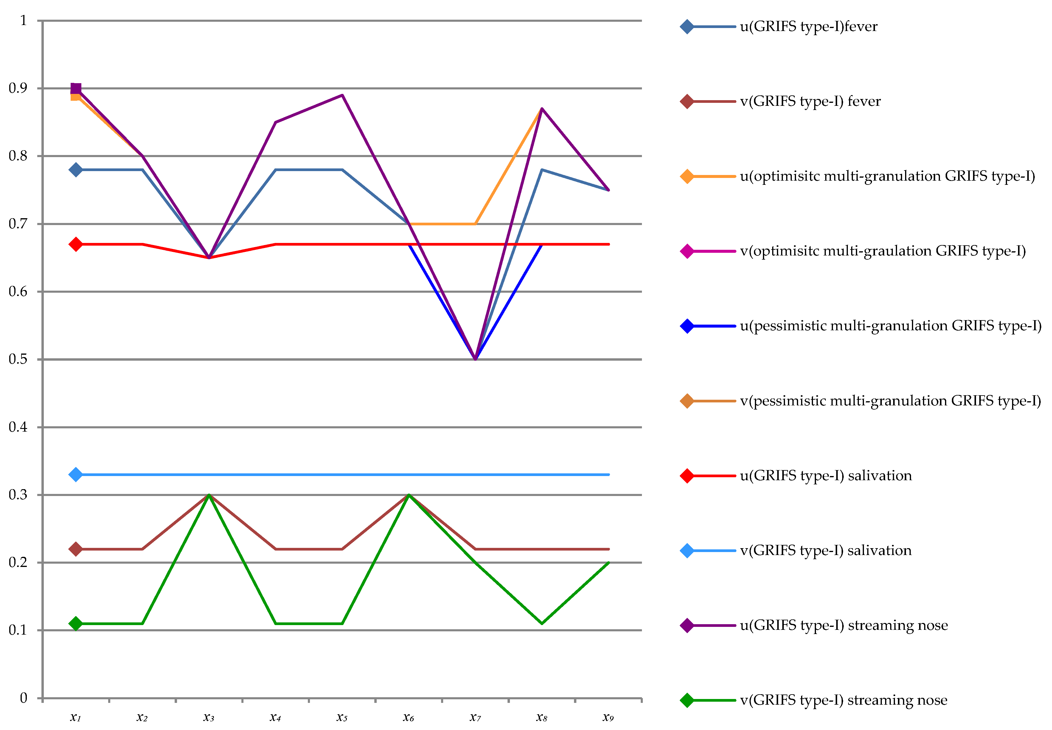
For Figure 1, we can obtain,

$$\begin{gathered} \mu {(y)}_{OI1}\ge \mu {(y)}_{GIn1}\mathrm{\Theta }\mu {(y)}_{GIf1}\mathrm{\Theta }{(y)}_{GIs1}\ge \mu {(y)}_{PI1}, \\ \nu {(y)}_{GIs1}\ge \nu {(y)}_{PI1}\ge \nu {(y)}_{OI1}=\nu {(y)}_{GIf1}\ge \nu {(y)}_{GIn1}; \end{gathered}$$

Note:

$\mathrm{\Theta }$ represents $\le \mathrm{or}\ge$;

$\mu {(y)}_{GIf1}$ and $\nu {(y)}_{GIf1}$ represent GRIFS type-I dominance relation (fever);

$\mu {(y)}_{GIs1}$ and $\nu {(y)}_{GIs1}$ represent GRIFS type-I dominance relation (salivation);

$\mu {(y)}_{GIn1}$ and $\nu {(y)}_{GIn1}$ represent GRIFS type-I dominance relation (streaming nose);

$\mu {(y)}_{OI1}$ and $\nu {(y)}_{OI1}$ represent optimistic multi-granulation GRIFS type-I dominance relation;

$\mu {(y)}_{PI1}$ and $\nu {(y)}_{PI1}$ represent pessimistic multi-granulation GRIFS type-I dominance relation;

From Figure 1, we can get that x₁, x₂, x₄, x₅ and x₈ patients have the disease, and x₇ patients do not have the disease.

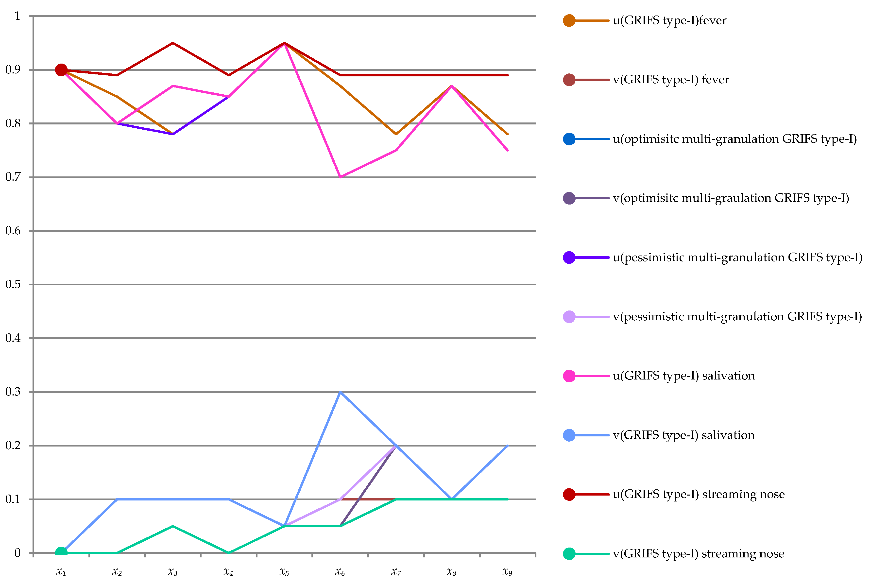
Then, from Figure 2, we can obtain,

$$\begin{gathered} \mu {(y)}_{O\mathrm{I}2}=\mu {(y)}_{G\mathrm{I}n2}\ge \mu {(y)}_{P\mathrm{I}2}\mathrm{\Theta }\mu {(y)}_{G\mathrm{I}s2}\mathrm{\Theta }\mu {(y)}_{G\mathrm{I}f2}, \\ \nu {(y)}_{G\mathrm{I}s2}\ge \nu {(y)}_{O\mathrm{I}2}\mathrm{\Theta }\nu {(y)}_{P\mathrm{I}2}\mathrm{\Theta }\nu {(y)}_{G\mathrm{I}f2}\ge \nu {(y)}_{G\mathrm{I}n2}; \end{gathered}$$

Note:

$\mathrm{\Theta }$ represents $\le \mathrm{or}\ge$;

$\mu {(y)}_{GIf2}$ and $\nu {(y)}_{GIf2}$ represent GRIFS type-I dominance relation (fever);

$\mu {(y)}_{GIs2}$ and $\nu {(y)}_{GIs2}$ represent GRIFS type-I dominance relation (salivation);

$\mu {(y)}_{GIn2}$ and $\nu {(y)}_{GIn2}$ represent GRIFS type-I dominance relation (streaming nose);

$\mu {(y)}_{OI2}$ and $\nu {(y)}_{OI2}$ represent optimistic multi-granulation GRIFS type-I dominance relation;

$\mu {(y)}_{PI2}$ and $\nu {(y)}_{PI2}$ represent pessimistic multi-granulation GRIFS type-I dominance relation;

From Figure 2, we can get that x₁, x₂, x₃, x₄, x₅, x₆, x₈, and x₉ patients have the disease, and x₆ patients do not have the disease.

For multi-granulation GRIFS models based on type-II dominance relation, the calculations for this model are similar to multi-granulation GRIFS models based on type-I dominance relation.

Firstly, for streaming nose, we can compute the disjunction operation of ${[x]}_a^{\ge }$ and ${[x]}_a^{{\ge }^{\prime }}$, and the results are as

Table 6. The disjunction operation of ${[x]}_a^{\ge }$ and ${[x]}_a^{{\ge }^{\prime }}$.

$\mathit{x}$	${\mathbf{[}\mathit{x}\mathbf{]}}_{\mathit{a}}^{\mathbf{\ge }}$	${\mathbf{[}\mathit{x}\mathbf{]}}_{\mathit{a}}^{\mathbf{\ge }\mathbf{\prime }}$	${\mathbf{[}\mathit{x}\mathbf{]}}_{\mathit{a}}^{\mathbf{\ge }}\mathbf{\vee }{\mathbf{[}\mathit{x}\mathbf{]}}_{\mathit{a}}^{\mathbf{\ge }\mathbf{\prime }}$
$x_1$	$\{x_1\},\{x_1,x_2,x_4\}$	$\{x_1\}$	$\{x_1,x_2,x_4\}$
$x_2$	$\{x_1,x_2,x_4\},\{x_2,x_7,x_8\}$	$\{x_2,x_4,x_5,x_8\}$	$\{x_1,x_2,x_4,x_5,x_7,x_8\}$
$x_3$	$\{x_3,x_5,x_6\}$	$\{x_3,x_4,x_5,x_6,x_8,x_9\}$	$\{x_3,x_4,x_5,x_6,x_8,x_9\}$
$x_4$	$\{x_1,x_2,x_4\},\{x_4,x_6,x_7,x_9\}$	$\{x_4,x_5\}$	$\{x_1,x_2,x_4,x_5,x_6,x_7,x_9\}$
$x_5$	$\{x_3,x_5,x_6\}$	$\{x_5\}$	$\{x_3,x_5,x_6\}$
$x_6$	$\{x_3,x_5,x_6\},\{x_4,x_6,x_7,x_9\}$	$\{x_6,x_8,x_9\}$	$\{x_3,x_4,x_5,x_6,x_7,x_8,x_9\}$
$x_7$	$\{x_2,x_7,x_8\},\{x_4,x_6,x_7,x_9\}$	$\{x_7,x_8,x_9\}$	$\{x_2,x_4,x_6,x_7,x_8,x_9\}$
$x_8$	$\{x_2,x_7,x_8\}$	$\{x_8\}$	$\{x_2,x_7,x_8\}$
$x_9$	$\{x_4,x_6,x_7,x_9\}$	$\{x_9\}$	$\{x_4,x_6,x_7,x_9\}$

.

Next, for salivation, we can compute the disjunction operation of ${[x]}_a^{\ge }$ and ${[x]}_a^{{\ge }^{\prime }}$, and the results are as

Table 7. The disjunction operation of ${[x]}_a^{\ge }$ and ${[x]}_a^{{\ge }^{\prime }}$.

$\mathit{x}$	${\mathbf{[}\mathit{x}\mathbf{]}}_{\mathit{a}}^{\mathbf{\ge }}$	${\mathbf{[}\mathit{x}\mathbf{]}}_{\mathit{a}}^{\mathbf{\ge }\mathbf{\prime }}$	${\mathbf{[}\mathit{x}\mathbf{]}}_{\mathit{a}}^{\mathbf{\ge }}\mathbf{\vee }{\mathbf{[}\mathit{x}\mathbf{]}}_{\mathit{a}}^{\mathbf{\ge }\mathbf{\prime }}$
$x_1$	$\{x_1,x_2\}$	$\{x_1\}$	$\{x_1,x_2\}$
$x_2$	$\{x_1,x_2\},\{x_2,x_4\}$	$\{x_2,x_4,x_5,x_8\}$	$\{x_1,x_2,x_4,x_5,x_8\}$
$x_3$	$\{x_3,x_8\}$	$\{x_3,x_4,x_5,x_6,x_8,x_9\}$	$\{x_3,x_4,x_5,x_6,x_8,x_9\}$
$x_4$	$\{x_2,x_4\}$	$\{x_4,x_5\}$	$\{x_2,x_4,x_5\}$
$x_5$	$\{x_5,x_6\}$	$\{x_5\}$	$\{x_5,x_6\}$
$x_6$	$\{x_5,x_6\}$	$\{x_6,x_8,x_9\}$	$\{x_5,x_6,x_8,x_9\}$
$x_7$	$\{x_7,x_9\},\{x_7,x_8,x_9\}$	$\{x_7,x_8,x_9\}$	$\{x_7,x_8,x_9\}$
$x_8$	$\{x_3,x_8\},\{x_7,x_8,x_9\}$	$\{x_8\}$	$\{x_3,x_7,x_8,x_9\}$
$x_9$	$\{x_7,x_9\},\{x_7,x_8,x_9\}$	$\{x_9\}$	$\{x_7,x_8,x_9\}$

.

Then, for fever, we compute the disjunction operation of ${[x]}_a^{\ge }$ and ${[x]}_a^{{\ge }^{\prime }}$, and these results are shown as

Table 8. The disjunction operation of ${[x]}_a^{\ge }$ and ${[x]}_a^{{\ge }^{\prime }}$.

$\mathit{x}$	${\mathbf{[}\mathit{x}\mathbf{]}}_{\mathit{a}}^{\mathbf{\ge }}$	${\mathbf{[}\mathit{x}\mathbf{]}}_{\mathit{a}}^{\mathbf{\ge }\mathbf{\prime }}$	${\mathbf{[}\mathit{x}\mathbf{]}}_{\mathit{a}}^{\mathbf{\ge }}\mathbf{\vee }{\mathbf{[}\mathit{x}\mathbf{]}}_{\mathit{a}}^{\mathbf{\ge }\mathbf{\prime }}$
$x_1$	$\{x_1,x_2,x_4\}$	$\{x_1\}$	$\{x_1,x_2,x_4\}$
$x_2$	$\{x_1,x_2,x_4\}$	$\{x_2,x_4,x_5,x_8\}$	$\{x_1,x_2,x_4,x_5,x_8\}$
$x_3$	$\{x_3,x_8\}$	$\{x_3,x_4,x_5,x_6,x_8,x_9\}$	$\{x_3,x_4,x_5,x_6,x_8,x_9\}$
$x_4$	$\{x_1,x_2,x_4\},\{x_4,x_5,x_6,x_9\}$	$\{x_4,x_5\}$	$\{x_1,x_2,x_4,x_5,x_6,x_9\}$
$x_5$	$\{x_4,x_5,x_6,x_9\}$	$\{x_5\}$	$\{x_4,x_5,x_6,x_9\}$
$x_6$	$\{x_4,x_5,x_6,x_9\}$	$\{x_6,x_8,x_9\}$	$\{x_4,x_5,x_6,x_8,x_9\}$
$x_7$	$\{x_7\}$	$\{x_7,x_8,x_9\}$	$\{x_7,x_8,x_9\}$
$x_8$	$\{x_3,x_8\}$	$\{x_8\}$	$\{x_3,x_8\}$
$x_9$	$\{x_4,x_5,x_6,x_9\}$	$\{x_9\}$	$\{x_4,x_5,x_6,x_9\}$

.

For streaming nose, we can get GRIFS based on type-II dominance relation,

$$\begin{array}{l}{\underset{\_}{R}}_1^{{\ge }^{\mathrm{\Pi }}}(B)=\{\frac{[0.8,0.11]}{x_1},\frac{[0.5,0.2]}{x_2},\frac{[0.65,0.3]}{x_3},\frac{[0.5,0.3]}{x_4},\frac{[0.65,0.3]}{x_5},\frac{[0.5,0.3]}{x_6},\frac{[0.5,0.3]}{x_7},\frac{[0.5,0.2]}{x_8},\frac{[0.5,0.3]}{x_9}\},\\ {\overline{R}}_1^{{\ge }^{\mathrm{\Pi }}}(B)=\{\frac{[0.9,0]}{x_1},\frac{[0.95,0]}{x_2},\frac{[0.95,0.05]}{x_3},\frac{[0.95,0]}{x_4},\frac{[0.95,0.05]}{x_5},\frac{[0.95,0.05]}{x_6},\frac{[0.89,0.1]}{x_7},\frac{[0.89,0.1]}{x_8},\frac{[0.89,0.1]}{x_9}\}.\end{array}$$

For salivation, we can get GRIFS based on type-II dominance relation,

$$\begin{array}{l}{\underset{\_}{R}}_1^{{\ge }^{\mathrm{\Pi }}}(B)=\{\frac{[0.67,0.33]}{x_1},\frac{[0.67,0.33]}{x_2},\frac{[0.65,0.33]}{x_3},\frac{[0.67,0.33]}{x_4},\frac{[0.67,0.33]}{x_5},\frac{[0.67,0.33]}{x_6},\frac{[0.5,0.33]}{x_7},\frac{[0.5,0.33]}{x_8},\\ \frac{[0.5,0.33]}{x_9}\},\\ {\overline{R}}_1^{{\ge }^{\mathrm{\Pi }}}(B)=\{\frac{[0.9,0]}{x_1},\frac{[0.95,0]}{x_2},\frac{[0.95,0.05]}{x_3},\frac{[0.95,0.05]}{x_4},\frac{[0.95,0.05]}{x_5},\frac{[0.95,0.05]}{x_6},\frac{[0.87,0.1]}{x_7},\frac{[0.87,0.1]}{x_8},\frac{[0.87,0.1]}{x_9}\}.\end{array}$$

For fever, GRIFS type-II dominance relation can be calculated as follows:

$$\begin{gathered} {\underset{\_}{R}}_1^{{\ge }^{\mathrm{\Pi }}}(B)=\{\frac{[0.78,0.22]}{x_1},\frac{[0.78,0.22]}{x_2},\frac{[0.65,0.3]}{x_3},\frac{[0.7,0.22]}{x_4},\frac{[0.7,0.22]}{x_5},\frac{[0.7,0.3]}{x_6},\frac{[0.5,0.22]}{x_7},\frac{[0.65,0.3]}{x_8},\frac{[0.7,0.3]}{x_9}\}, \\ {\overline{R}}_1^{{\ge }^{\mathrm{\Pi }}}(B)=\{\frac{[0.9,0]}{x_1},\frac{[0.95,0]}{x_2},\frac{[0.95,0.05]}{x_3},\frac{[0.95,0]}{x_4},\frac{[0.95,0.05]}{x_5},\frac{[0.95,0.05]}{x_6},\frac{[0.87,0.1]}{x_7},\frac{[0.87,0.1]}{x_8},\frac{[0.95,0.05]}{x_9}\}. \end{gathered}$$

Based on Definitions 13 and 14, the condition of these patients based on multi-granulation GRIFS type-II dominance relation can be obtained as follows:

$$\begin{array}{l}{\underset{\_}{{\displaystyle \sum _{i=1}^3{R}_{A_i}^O}}}_1^{{\ge }^{\mathrm{\Pi }}}(B)=\{\frac{[0.8,0.11]}{x_1},\frac{[0.78,0.2]}{x_2},\frac{[0.65,0.3]}{x_3},\frac{[0.7,0.22]}{x_4},\frac{[0.7,0.3]}{x_5},\frac{[0.7,0.3]}{x_6},\frac{[0.5,0.22]}{x_7},\frac{[0.65,0.2]}{x_8},\frac{[0.7,0.3]}{x_9}\},\\ {\overline{{\displaystyle \sum _{i=1}^3{R}_{A_i}^O}}}_1^{{\ge }^{\mathrm{\Pi }}}(B)=\{\frac{[0.9,0]}{x_1},\frac{[0.95,0]}{x_2},\frac{[0.95,0.05]}{x_3},\frac{[0.95,0.05]}{x_4},\frac{[0.95,0.05]}{x_5},\frac{[0.95,0.05]}{x_6},\frac{[0.87,0.1]}{x_7},\frac{[0.87,0.1]}{x_8},\frac{[0.87,0.1]}{x_9}\}.\\ {\underset{\_}{{\displaystyle \sum _{i=1}^3{R}_{A_i}^P}}}_1^{{\ge }^{\mathrm{\Pi }}}(B)=\{\frac{[0.67,0.33]}{x_1},\frac{[0.5,0.33]}{x_2},\frac{[0.65,0.33]}{x_3},\frac{[0.5,0.4]}{x_4},\frac{[0.65,0.33]}{x_5},\frac{[0.5,0.33]}{x_6},\frac{[0.5,0.33]}{x_7},\frac{[0.5,0.33]}{x_8},\frac{[0.5,0.33]}{x_9}\},\\ {\overline{{\displaystyle \sum _{i=1}^3{R}_{A_i}^P}}}_1^{{\ge }^{\mathrm{\Pi }}}(B)=\{\frac{[0.9,0]}{x_1},\frac{[0.95,0]}{x_2},\frac{[0.95,0.05]}{x_3},\frac{[0.95,0]}{x_4},\frac{[0.95,0.05]}{x_5},\frac{[0.95,0.05]}{x_6},\frac{[0.89,0.1]}{x_7},\frac{[0.89,0.1]}{x_8},\frac{[0.95,0.05]}{x_9}\}.\end{array}$$

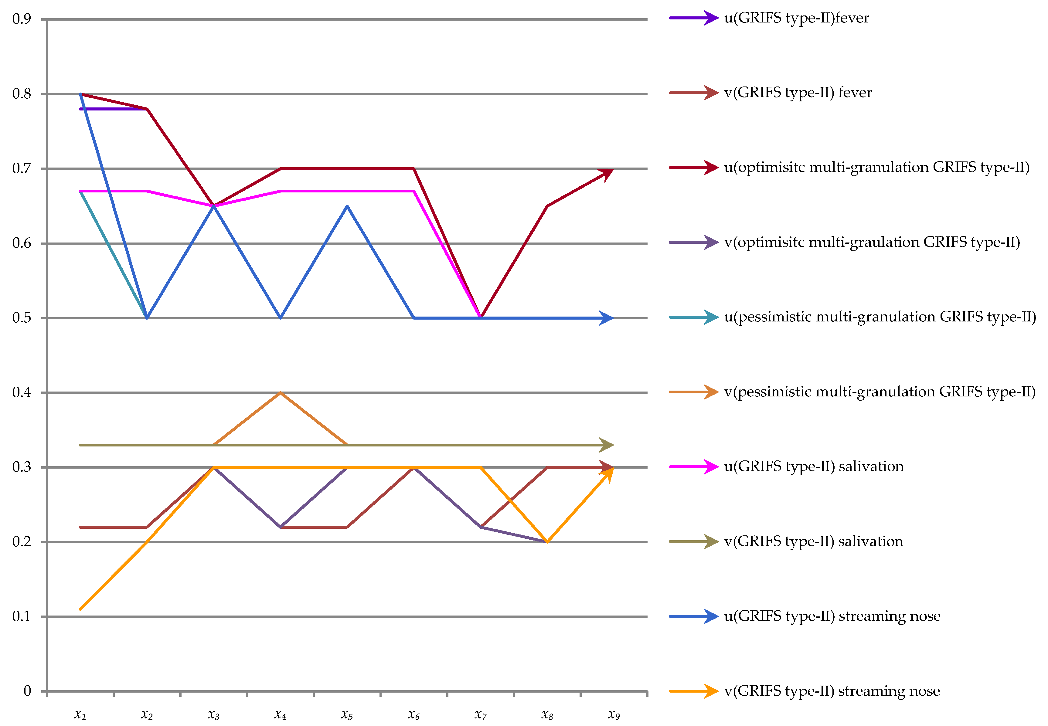
Then, from Figure 3, we can obtain,

$$\begin{gathered} \mu {(y)}_{O\mathrm{\Pi }3}\ge \mu {(y)}_{G\mathrm{\Pi }f3}\mathrm{\Theta }\mu {(y)}_{G\mathrm{\Pi }n3}\mathrm{\Theta }\mu {(y)}_{G\mathrm{\Pi }s3}\ge \mu {(y)}_{P\mathrm{\Pi }3}, \\ \nu {(y)}_{P\mathrm{\Pi }3}\ge \nu {(y)}_{G\mathrm{\Pi }s3}\mathrm{\Theta }\nu {(y)}_{O\mathrm{\Pi }3}\mathrm{\Theta }\nu {(y)}_{G\mathrm{\Pi }f3}\mathrm{\Theta }\nu {(y)}_{G\mathrm{\Pi }n3}; \end{gathered}$$

Note:

$\mathrm{\Theta }$ represents $\le \mathrm{or}\ge$;

$\mu {(y)}_{G\mathrm{\Pi }f3}$ and $\nu {(y)}_{G\mathrm{\Pi }f3}$ represent GRIFS type-II dominance relation (fever);

$\mu {(y)}_{G\mathrm{\Pi }s3}$ and $\nu {(y)}_{G\mathrm{\Pi }s3}$ represent GRIFS type-II dominance relation (salivation);

$\mu {(y)}_{G\mathrm{\Pi }n3}$ and $\nu {(y)}_{G\mathrm{\Pi }n3}$ represent GRIFS type-II dominance relation (streaming nose);

$\mu {(y)}_{O\mathrm{\Pi }3}$ and $\nu {(y)}_{O\mathrm{\Pi }3}$ represent optimistic multi-granulation GRIFS type-II dominance relation;

$\mu {(y)}_{P\mathrm{\Pi }3}$ and $\nu {(y)}_{P\mathrm{\Pi }3}$ represent pessimistic multi-granulation GRIFS type-II dominance relation;

From Figure 3, we can see that x₁, x₂, x₄ patients have the disease, and x₃, x₅, x₆, x₇, x₈, x₉ patients do not have the disease.

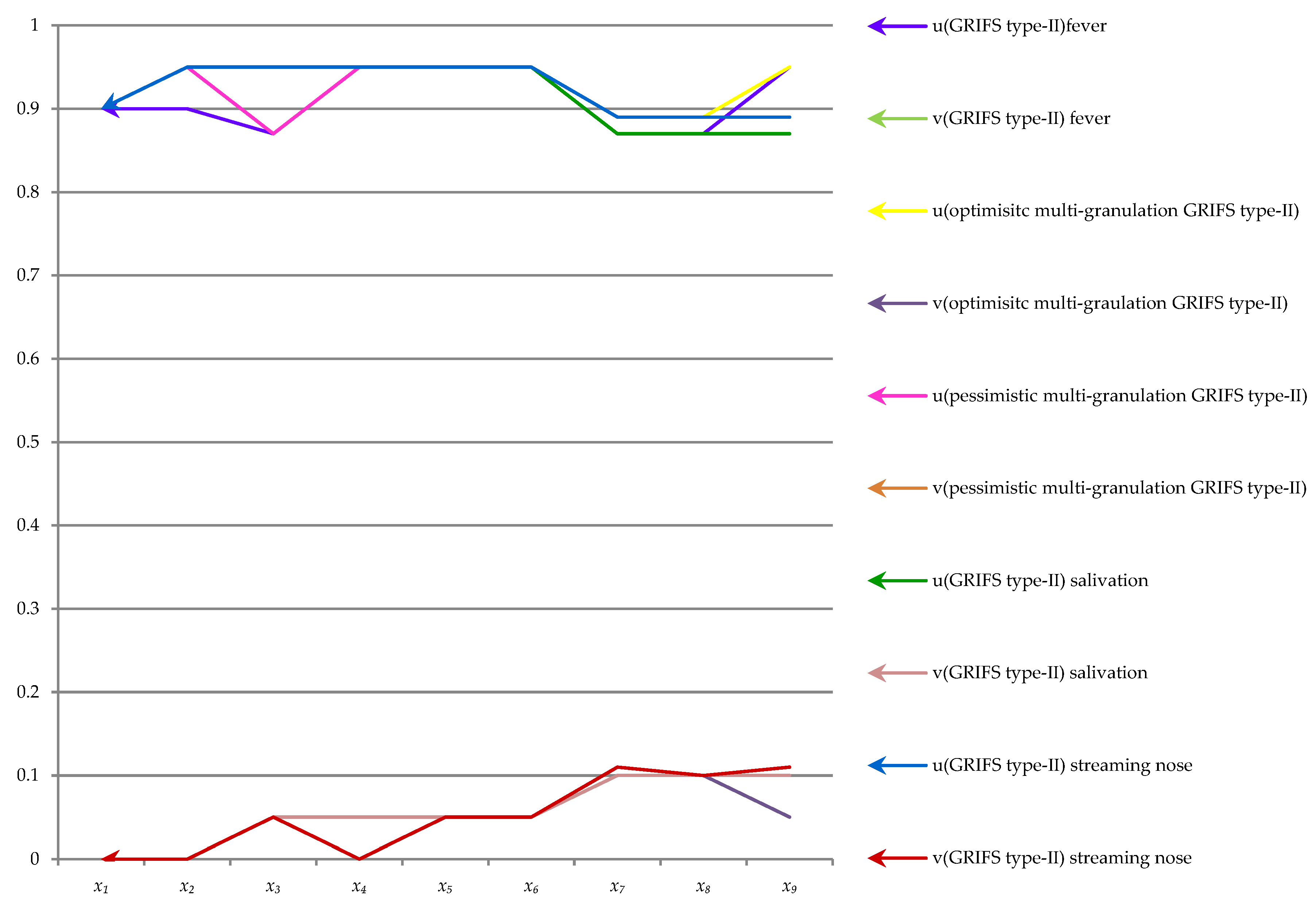
Then, from Figure 4, we can obtain,

$$\begin{gathered} \mu {(y)}_{O\mathrm{\Pi }4}\ge \mu {(y)}_{G\mathrm{\Pi }n4}\mathrm{\Theta }\mu {(y)}_{G\mathrm{\Pi }f4}\mathrm{\Theta }\mu {(y)}_{G\mathrm{\Pi }s4}\ge \mu {(y)}_{P\mathrm{\Pi }4}, \\ \nu {(y)}_{P\mathrm{\Pi }4}\mathrm{\Theta }\nu {(y)}_{G\mathrm{\Pi }s4}\mathrm{\Theta }\nu {(y)}_{G\mathrm{\Pi }f4}\mathrm{\Theta }\nu {(y)}_{G\mathrm{\Pi }n4}\mathrm{\Theta }\nu {(y)}_{O\mathrm{\Pi }4}; \end{gathered}$$

Note:

$\mathrm{\Theta }$ represents $\le \mathrm{or}\ge$;

$\mu {(y)}_{G\mathrm{\Pi }f4}$ and $\nu {(y)}_{G\mathrm{\Pi }f4}$ represent GRIFS type-II dominance relation (fever);

$\mu {(y)}_{G\mathrm{\Pi }s4}$ and $\nu {(y)}_{G\mathrm{\Pi }s4}$ represent GRIFS type-II dominance relation (salivation);

$\mu {(y)}_{G\mathrm{\Pi }n4}$ and $\nu {(y)}_{G\mathrm{\Pi }n4}$ represent GRIFS type-II dominance relation (streaming nose);

$\mu {(y)}_{O\mathrm{\Pi }4}$ and $\nu {(y)}_{O\mathrm{\Pi }4}$ represent optimistic multi-granulation GRIFS type-II dominance relation;

$\mu {(y)}_{P\mathrm{\Pi }4}$ and $\nu {(y)}_{P\mathrm{\Pi }4}$ represent pessimistic multi-granulation GRIFS type-II dominance relation;

From Figure 4, we can see that x₁, x₂, x₃, x₄, x₅, x₆, x₇, x₈ and x₉ patients have the disease.

From Figure 1 and Figure 2, x₁, x₂, x₄ and x₈ patients have the disease, x₆ and x₇ patient do not have the disease. From Figure 3 and Figure 4, x₁, x₂ and x₄ patients have the disease, x₃, x₅, x₆, x₇, x₈ and x₉ patients do not have the disease. Furthermore, this example proves the accuracy of Algorithm 1.

This example analyzes and discusses multi-granulation GRIFS models based on dominance relation. From conjunction and disjunction operations of two kinds of dominance classes perspective, we analyzed GRIFS models based on type-I dominance relation and type-II dominance relation and also optimistic and pessimistic multi-granulation GRIFS models based on type-I dominance relation and type-II dominance relation, respectively. Through the analysis of this example, the validity of these multi-granulation GRIFS models based on type-I dominance relation and type-II dominance relation models can be obtained.

6. Conclusions

These theories of GRS and RIFS are extensions of the classical rough set theory. In this paper, we proposed a series of models on GRIFS based on dominance relation, which were based on the combination of GRS, RIFS, and dominance relations. Moreover, these models of multi-granulation GRIFS models based on dominance relation were established on GRIFS models based on dominance relation using multiple dominance relations on the universe. The validity of these models was demonstrated by giving examples. Compared with GRS based on dominance relation, GRIFS models based on dominance relation can be more precise. Compared with GRIFS models based on dominance relation, multi-granulation GRIFS models based on dominance relation can be more accurate. It can be demonstrated using the algorithm, and our methods provide a way to combine GRS and RIFS. Our next work is to study the combination of GRS and variable precision rough sets on the basis of our proposed methods.

References

- Pawlak, Z. Rough sets. Int. J. Comput. Inf. Sci. 1982, 11, 341–356. [Google Scholar] [CrossRef]
- Yao, Y.Y.; Lin, T.Y. Generalization of rough sets using modal logics. Intell. Autom. Soft Comput. 1996, 2, 103–119. [Google Scholar] [CrossRef]
- Zhang, X.Y.; Mo, Z.W.; Xiong, F.; Cheng, W. Comparative study of variable precision rough set model and graded rough set model. Int. J. Approx. Reason. 2012, 53, 104–116. [Google Scholar] [CrossRef]
- Zadeh, L.A. Fuzzy Sets, Fuzzy Logic, and Fuzzy Systems; World Scientific Publishing Corporation: Singapore, 1996; pp. 433–448. [Google Scholar]
- Qian, Y.H.; Liang, J.Y.; Yao, Y.Y.; Dang, C.Y. MGRS: A multi-granulation rough set. Inf. Sci. 2010, 180, 949–970. [Google Scholar] [CrossRef]
- Xu, W.H.; Wang, Q.R.; Zhang, X.T. Multi-granulation fuzzy rough sets in a fuzzy tolerance approximation space. Int. J. Fuzzy Syst. 2011, 13, 246–259. [Google Scholar]
- Lin, G.P.; Liang, J.Y.; Qian, Y.H. Multigranulation rough sets: From partition to covering. Inf. Sci. 2013, 241, 101–118. [Google Scholar] [CrossRef]
- Liu, C.H.; Pedrycz, W. Covering-based multi-granulation fuzzy rough sets. J. Intell. Fuzzy Syst. 2015, 30, 303–318. [Google Scholar] [CrossRef]
- Xue, Z.A.; Si, X.M.; Xue, T.Y.; Xin, X.W.; Yuan, Y.L. Multi-granulation covering rough intuitionistic fuzzy sets. J. Intell. Fuzzy Syst. 2017, 32, 899–911. [Google Scholar]
- Hu, Q.J. Extended Graded Rough Sets Models Based on Covering. Master’s Thesis, Shanxi Normal University, Linfen, China, 21 March 2016. (In Chinese). [Google Scholar]
- Wang, H.; Hu, Q.J. Multi-granulation graded covering rough sets. In Proceedings of the International Conference on Machine Learning and Cybernetics, Guangzhou, China, 12–15 July 2015; Institute of Electrical and Electronics Engineers Computer Society: New York, NY, USA, 2015. [Google Scholar]
- Wu, Z.Y.; Zhong, P.H.; Hu, J.G. Graded multi-granulation rough sets. Fuzzy Syst. Math. 2014, 28, 165–172. (In Chinese) [Google Scholar]
- Yu, J.H.; Zhang, X.Y.; Zhao, Z.H.; Xu, W.H. Uncertainty measures in multi-granulation with different grades rough set based on dominance relation. J. Intell. Fuzzy Syst. 2016, 31, 1133–1144. [Google Scholar] [CrossRef]
- Yu, J.H.; Xu, W.H. Multigranulation with different grades rough set in ordered information system. In Proceedings of the International Conference on Fuzzy Systems and Knowledge Discovery, Zhangjiajie, China, 15–17 August 2015; Institute of Electrical and Electronics Engineers Incorporated: New York, NY, USA, 2016. [Google Scholar]
- Wang, X.Y.; Shen, J.Y.; Shen, J.L.; Shen, Y.X. Graded multi-granulation rough set based on weighting granulations and dominance relation. J. Shandong Univ. 2017, 52, 97–104. (In Chinese) [Google Scholar]
- Zheng, Y. Graded multi-granularity rough sets based on covering. J. Shanxi Normal Univ. 2017, 1, 5–9. (In Chinese) [Google Scholar]
- Shen, J.R.; Wang, X.Y.; Shen, Y.X. Variable grade multi-granulation rough set. J. Chin. Comput. Syst. 2016, 37, 1012–1016. (In Chinese) [Google Scholar]
- Atanassov, K.T.; Rangasamy, P. Intuitionistic fuzzy sets. Fuzzy Sets Syst. 1986, 20, 87–96. [Google Scholar] [CrossRef]
- Zadeh, L.A. Fuzzy sets. Inf. Control 1965, 8, 338–353. [Google Scholar] [CrossRef] [Green Version]
- Huang, B.; Zhuang, Y.L.; Li, H.X. Information granulation and uncertainty measures in interval-valued intuitionistic fuzzy information systems. Eur. J. Oper. Res. 2013, 231, 162–170. [Google Scholar] [CrossRef]
- Slowinski, R.; Vanderpooten, D. A generalized definition of rough approximations based on similarity. IEEE Trans. Knowl. Data Eng. 1996, 12, 331–336. [Google Scholar] [CrossRef]
- Chang, K.H.; Cheng, C.H. A risk assessment methodology using intuitionistic fuzzy set in FMEA. Int. J. Syst. Sci. 2010, 41, 1457–1471. [Google Scholar] [CrossRef]
- Zhang, X.H. Fuzzy anti-grouped filters and fuzzy normal filters in pseudo-BCI algebras. J. Intell. Fuzzy Syst. 2017, 33, 1767–1774. [Google Scholar] [CrossRef]
- Gong, Z.T.; Zhang, X.X. The further investigation of variable precision intuitionistic fuzzy rough set model. Int. J. Mach. Learn. Cybern. 2016, 8, 1565–1584. [Google Scholar] [CrossRef]
- He, Y.P.; Xiong, L.L. Generalized inter-valued intuitionistic fuzzy soft rough set and its application. J. Comput. Anal. Appl. 2017, 23, 1070–1088. [Google Scholar]
- Zhang, X.H.; Bo, C.X.; Smarandache, F.; Dai, J.H. New inclusion relation of neutrosophic sets with applications and related lattice structure. Int. J. Mach. Learn. Cybern. 2018, 9, 1753–1763. [Google Scholar] [CrossRef]
- Zhang, X.H.; Smarandache, F.; Liang, X.L. Neutrosophic duplet semi-group and cancellable neutrosophic triplet groups. Symmetry 2017, 9, 275. [Google Scholar] [CrossRef]
- Huang, B.; Guo, C.X.; Li, H.X.; Feng, G.F.; Zhou, X.Z. An intuitionistic fuzzy graded covering rough set. Knowl.-Based Syst. 2016, 107, 155–178. [Google Scholar] [CrossRef]
- Tiwari, A.K.; Shreevastava, S.; Som, T. Tolerance-based intuitionistic fuzzy-rough set approach for attribute reduction. Expert Syst. Appl. 2018, 101, 205–212. [Google Scholar] [CrossRef]
- Guo, Q.; Ming, Y.; Wu, L. Dominance relation and reduction in intuitionistic fuzzy information system. Syst. Eng. Electron. 2014, 36, 2239–2243. [Google Scholar]
- Ai, A.H.; Xu, Z.S. Line integral of intuitionistic fuzzy calculus and their properties. IEEE Trans. Fuzzy Syst. 2018, 26, 1435–1446. [Google Scholar] [CrossRef]
- Rizvi, S.; Naqvi, H.J.; Nadeem, D. Rough intuitionistic fuzzy sets. In Proceedings of the 6th Joint Conference on Information Sciences, Research Triangle Park, NC, USA, 8–13 March 2002; Duke University/Association for Intelligent Machinery: Durham, NC, USA, 2002. [Google Scholar]
- Zhang, X.X.; Chen, D.G.; Tsang, E.C.C. Generalized dominance rough set models for the dominance intuitionistic fuzzy information systems. Inf. Sci. 2017, 378, 1339–1351. [Google Scholar] [CrossRef]
- Zhang, Y.Q.; Yang, X.B. An intuitionistic fuzzy dominance-based rough set. In Proceedings of the 7th International Conference on Intelligent Computing, Zhengzhou, China, 11–14 August 2011; Springer: Berlin, Germany, 2011. [Google Scholar]
- Huang, B.; Zhuang, Y.L.; Li, H.X.; Wei, D.K. A dominance intuitionistic fuzzy-rough set approach and its applications. Appl. Math. Model. 2013, 37, 7128–7141. [Google Scholar] [CrossRef]
- Zhang, W.X.; Wu, W.Z.; Liang, J.Y.; Li, D.Y. Theory and Method of Rough Sets; Science Press: Beijing, China, 2001. (In Chinese) [Google Scholar]
- Wen, X.J. Uncertainty measurement for intuitionistic fuzzy ordered information system. Master’s Thesis, Shanxi Normal University, Linfen, China, 21 March 2015. (In Chinese). [Google Scholar]
- Lezanski, P.; Pilacinska, M. The dominance-based rough set approach to cylindrical plunge grinding process diagnosis. J. Intell. Manuf. 2018, 29, 989–1004. [Google Scholar] [CrossRef]
- Huang, B.; Guo, C.X.; Zhang, Y.L.; Li, H.X.; Zhou, X.Z. Intuitionistic fuzzy multi-granulation rough sets. Inf. Sci. 2014, 277, 299–320. [Google Scholar] [CrossRef]
- Greco, S.; Matarazzo, B.; Slowinski, R. An algorithm for induction decision rules consistent with the dominance principle. In Proceedings of the 2nd International Conference on Rough Sets and Current Trends in Computing, Banff, AB, Canada, 16–19 October 2000; Springer: Berlin, Germany, 2011. [Google Scholar]
Figure 1.
The lower approximation of GRIFS based on type-I dominance relation, as well as optimistic and pessimistic multi-granulation GRIFS based on type-I dominance relation.
Figure 2.
The upper approximation of GRIFS based on type-I dominance relation, as well as optimistic and pessimistic multi-granulation GRIFS based on type-I dominance relation.
Figure 3.
The lower approximation of GRIFS based on type-II dominance relation, as well as optimistic and pessimistic multi-granulation GRIFS based on type-II dominance relation.
Figure 4.
The upper approximation of GRIFS based on type-II dominance relation, as well as optimistic and pessimistic multi-granulation GRIFS based on type-II dominance relation.