Spatial Variations and Determinants of Per Capita Household CO2 Emissions (PHCEs) in China
by
 ,
,
Lina Liu
1 ,
,
Jiansheng Qu
1,2,*,
Afton Clarke-Sather
2,3,
Tek Narayan Maraseni
4 and
Jiaxing Pang
1 1
Key Laboratory of Western China’s Environmental Systems, College of Earth and Environmental Sciences, Lanzhou University, Lanzhou 730000, China
2
Information Center for Global Change Studies, Lanzhou Information Center, Chinese Academy of Sciences, Lanzhou 730000, China
3
Department of Geography, University of Delaware, Newark, DE 19716, USA
4
Institute for Agriculture and the Environment, University of Southern Queensland, Toowoomba, QLD 4350, Australia
*
Author to whom correspondence should be addressed.
Sustainability 2017, 9(7), 1277; https://doi.org/10.3390/su9071277
Submission received: 19 June 2017
/
Revised: 17 July 2017
/
Accepted: 18 July 2017
/
Published: 20 July 2017
Abstract
:In China, household CO2 emissions (HCEs) are increasing due to economic development and accelerated urbanization. This paper details the spatial variations of per capita household CO2 emissions (PHCEs) in China and the factors impacting PHCEs using spatial statistical analysis and a spatial panel data model for the period from 1997 to 2014. Our results indicate that (1) there has been high provincial variation in rates of change across China, with some provinces’ PHCEs increasing by an order of magnitude from 1997 to 2014; (2) the Global Moran’s I of PHCEs are above 0, and the spatial differences between PHCEs are caused by the High-High cluster and Low-Low cluster in China; (3) a 1% increase of per capita income, education level, and urbanization will result in increases in PHCEs of 0.6990%, 0.0149%, and 0.0044%, respectively, whilst a 1% increase in household size will result in a 0.0496% decrease in PHCEs. There are a large number of factors impacting CO2 emissions, while there is little specific guidance on the spatial variations and provincial characteristics of CO2 emissions from the perspective of household consumption.
1. Introduction
Global climate change is primarily caused by anthropogenic greenhouse gas emissions, particularly CO2 emissions [1,2]. China is currently the largest CO2 emitter in the world and continues to have rapid growth in CO2 emissions [3]. Facing fast-growing CO2 emissions, the Chinese government established a goal of reducing its carbon intensity to 40% to 50% of 2005 levels by 2020 at the Copenhagen Climate Conference in 2009 and vowed to reach its carbon emissions peak circa 2030 and make efforts to peak early during the APEC (Asia-Pacific Economic Cooperation) Summit in 2014. While many of these emissions can be attributed to household energy usage, household consumption will account for a rising portion of emissions in the coming decades as living standards improve [4,5,6]. Early evaluations of carbon emission reduction efforts focused on the industrial sector and evaluated CO2 emissions from fossil fuels, but, recently, researchers have turned to studies of CO2 emissions from household consumption [4,6,7,8,9,10,11], with per capita household CO2 emissions (PHCEs) being an important point for climate change mitigation efforts in the future [12].
Previous studies of household CO2 emissions (HCEs) can be divided into three phases. During the initial phase (1990 to 2000), scholars focused on analyzing carbon emissions from residential uses [13,14,15]. The second phase (2001 to 2010) featured the development of a variety of assessment methods for carbon emissions from household consumption, including the Consumer Lifestyle Approach [16,17], the IPCC Reference Approach (IPCC Reference Approach for estimating CO2 emissions) [1,18], and Input-output analysis [19,20]. In addition, household CO2 emissions were divided into direct and indirect carbon emissions for the purpose of analysis [16,17,20]. The third phase (2011 to the present) has seen the focus shift to the analysis of factors influencing household CO2 emissions and measures to reduce CO2 emissions.
Studies of factors influencing HCEs have used a variety of approaches, including Logarithmic Mean Divisia Index (LMDI) models [21,22,23], Stochastic Impacts by Regression on Population, Affluence and Technology (STIRPAT) models [24,25], shapley decomposition [26], Structural Decomposition Analysis (SDA) models [27], self-organizing feature map (SOFM) models [28], the Adaptive Weighting Divisia (AWD) method [29], and multivariate analysis [30]. Although many scholars have explored how household carbon emissions and the factors influencing their variation vary across time, few have explored the spatial variations of PHCEs and their influencing factors. This paper contributes to the understanding of the factors influencing PHCEs by evaluating spatial patterns.
In China, there is a rich source of literature on the spatial analysis of CO2 emissions from energy consumption [31,32,33]. Based on Chinese provincial energy consumption data, Chuai et al. [31] identified an increasing trend in the global spatial autocorrelation in carbon emissions. Similarly, for carbon intensity, a growing spatial agglomeration based on Moran’s I has been identified [32]. However, energy usage and CO2 emissions from the household sector accounted for 27% and 17%, respectively, of total global emissions [34]. In China, estimates of CO2 emissions from households range from 35% [6] to 40% [4] of total emissions. To develop national and regional carbon reduction targets for the future, it is essential to analyze the factors influencing household CO2 emissions for residents in China by using a spatial perspective.
Recently, the relationship between CO2 emissions and the related influencing factors have been analyzed using spatial panel data models at the global level [35,36,37,38,39], national level [40,41], and provincial level [42,43,44,45]. There are numerous advantages to spatial panel data models, including improved efficiency with increasing degrees of freedom, the capability of controlling individual heterogeneity, and reduced the effects of collinearity among different variables [46]. Spatial panel data analysis has been used to examine the factors influencing carbon emissions both in spatial and temporal dimensions. For example, the relationship between economic development and CO2 emissions was investigated by Du et al. [42], and the relationship between urbanization, energy consumption, and carbon emissions was examined by Wang et al. [43]. Many factors affected CO2 emissions, including population, economic factors, and social variables. This study investigates the impacts of population, economic development, and technology on China’s PHCEs by constructing different forms of spatial panel data models, including pooled regression models and variable intercepts models with both constant and variable coefficients.
In this study, we compare PHCEs at the provincial level in China and their related influencing factors (e.g., population, economic status, and technology) using a spatial panel data model. The paper asks two questions. (1) What is the current distribution of PHCEs in China? We answer this through the spatial analysis of a data set of provincial level PHCEs using measures of both global and local spatial autocorrelation. (2) What factors have influenced this distribution of PHCEs? We answer this question through use of a panel model to estimate the effects of factors likely to influence PHCEs.
The remainder of this article is organized as follows. Section 2 presents the data sources and analytical methods. Section 3 evaluates the spatial distribution of PHCEs and discusses the influencing factors based on a spatial panel data method. Finally, in Section 4, we offer some conclusions and give primary policy recommendations related to PHCEs.
2. Research Methods and Data Sources
2.1. Estimation of PHCEs
PCHEs can be divided into six parts in this work: coal, oil, gas, other fuels, electricity, heating, and household consumption. Household CO2 emissions from coal, oil, gas, and other fuels are calculated based on the IPCC reference approach [1]. Household CO2 emissions from electricity and heating are calculated following the IPCC Reference Approach [1] and the National Development and Reform Commission (NDRC) [47]. This follows a ‘twelfth five-year’ control scheme for greenhouse gas emissions and includes the first ten industries in greenhouse gas emission accounting methods and reporting guidelines [47]. Household CO2 emissions from other household consumption are calculated by (1) Input-output analysis, which is similar to Bin and Dowlatabadi [16] and Wei et al. [17], and (2) the Consumer Lifestyle Approach, following Liu et al. [4], Zhu et al. [5], and Qu et al. [8,9]. In this work, we calculate the total amount of household CO2 emissions in China based on the provincial unit. The formula of calculating PHCEs in each province is shown below:
where ET is the total amount of household CO2 emissions in each Chinese province (t CO2); ECoal is the total amount of household CO2 emissions from coal usage (t CO2); EOil is the total amount of household CO2 emissions from oil usage (t CO2); EGas is the total amount of household CO2 emissions from gas usage (t CO2); EOther is the total amount of household CO2 emissions from the use of other fuels (t CO2); EElec is the total amount of household CO2 emissions from electricity usage (t CO2); EHeat is the total amount of household CO2 emissions from heating (heating usage in this study is the centralized heating usage in urban China; meanwhile, the centralized heating usage equals zero in rural China) (t CO2); and EHC is the total amount of household CO2 emissions from household consumption (t CO2).
where Fi denotes the fuel consumption of the average household (104 t/108 m3) (i = coal, oil, gas, and other fossil fuels); NCVi is the Net Calorific Value of the ith fuel (TJ/104 t/108 m3); CCi denotes the Carbon Emission Factor of the ith fuel (t C/TJ); OFi expresses the fraction of carbon oxidized for the ith fuel; and 44/12 is the ratio of molecular weight of CO2/C.
where FElec is the electric power consumption (MWh); CElec is the CO2 emission factor of the electricity sector (t CO2/MWh) from different provinces in 2010, which comes from the Baseline Emission Factor for provincial power grids in China [48]; FHeat (GJ) is the heating power consumption; and CHeat is the CO2 emissions factor of the heating sector (t CO2/GJ), which is derived from the NDRC [47].
where CHC = CDj(I − A)−1 and CDj = Ej/Pj, FIj is the consumption of the household (104 RMB); CHC is the CO2 emissions factor from household consumption (t CO2/104 RMB); j is the household consumption category (i.e., food, clothing, residence, household equipment, transportation and communication, cultural and educational entertainment, medical care, and other goods); CDj is the direct energy carbon emissions intensity from the jth category (t CO2/104 RMB); Ej is the direct energy carbon emissions from the jth category (t CO2, Ej is calculated based on Equation (2); Pj is the total output value of the jth category (104 RMB); A is the direct requirement matrix; I is the identity matrix; and (I − A)−1 is Leontief inverse square matrix.
where PHCEs is the per capita household CO2 emissions (t CO2/person) and P is the population size of each province in China.
2.2. The Spatial Statistical Analysis
2.2.1. Global Spatial Autocorrelation
Spatial autocorrelation and spatial regression analyses have long been employed in studies of energy consumption and the related carbon emissions [31,32,33]. In this study, changing trends in regional spatial patterns of PHCEs are evaluated by Global Moran’s I and Local Indicators of Spatial Association (LISA) by using ArcGIS10.3 and GeoDa software, respectively.
The formulas of Global Moran’s I are shown below [49]:
where ; n is the total number of provinces; xi and xj are the household carbon emissions of the ith and jth provinces, respectively; is the average of all observational values; and wij is the spatial weight matrix. In this study, we use the z value as Moran’s I statistic test, calculated as .
The Global Moran’s I measures the degree of global spatial autocorrelation for PHCEs in China, with values ranging between −1 and 1. Spatial autocorrelation is positive if the value is > 0, indicating more agglomeration, and negative for values < 0, indicating more scattered data. There is no spatial autocorrelation when the value is equal to 0 [49].
2.2.2. Cluster and Outlier Analysis
In addition to global spatial autocorrelation, this article examines the Local Indicators of Spatial Association (LISA) [49], expressed as:
where and .
LISA makes every local spatial unit a target item, which indicates the presence or absence of significant spatial clusters or outliers for every local spatial pattern. The Moran scatterplot can identify relationships between a local province and its adjacent provinces. By composing four quadrants [49], the upper right quadrant, termed High-High (H-H), and the lower left quadrant, termed Low-Low (L-L), indicate that there is a conglomeration effect of high values and low values between the province and its adjacent provinces, respectively. The upper left quadrant, termed High-Low (H-L), and the lower right quadrant, termed Low-High (L-H), indicate that the province itself has a high value with low values in adjacent provinces and that the province itself has a low value with high values in adjacent provinces, respectively.
2.2.3. The Standard Deviational Ellipse
The Standard Deviational Ellipse (SDE) is a Geographic Information Systems (GIS) tool for delineating the dispersion of univariate features around its center [50], which was initially put forward by Lefever [51]. We use the SDE to calculate the gravity center of PHCEs in China following Lefever [51] and Zhao and Zhao [50]. The center of SDE is calculated as:
where xi and yi are the space coordinates of each feature; and are the arithmetic average centers; and are the center of SDE; and , , and represent the angle of rotation, the length of X, and the length of Y of the SDE, respectively.
2.3. Spatial Panel Data Models
A spatial panel data analysis is used in this paper is to estimate the relationships between PHCEs and factors predicted to influence PHCEs. There are three types of panel data analytic models based on different parameters, as shown in Figure 1; pooled regression models (, variable intercepts and constant coefficient models (, and variable intercepts and variable coefficient models ( [46]. In Figure 1, yit is the index for the dependent variable; xit is the index for the independent variable; ai and bi are expressed as fixed effects or random effects; and is the error term. Baltagi [46] has shown that the Hausman test is the most appropriate analytic to select the suitability of spatial panel data models. In this work, we use the Hausman test to decide which model is most suitable for analyzing the factors influencing PHCEs in China.
Based on the Hausman test, two main hypotheses are used to confirm which specific model should be selected. The formulas are shown as below [46]:
where F2 is the statistic for H2; F1 is the statistic for H1; S1, S2, and S3 are the residual sums of the squares of the three spatial panel data models above, respectively; and N, T, and k are the number of entities, time points, and explanatory variables, respectively.
Based on these two hypotheses, if H2 is accepted, we should choose the pooled regression model. If H2 is rejected but H1 is accepted, we should choose the variable intercepts and constant coefficients model. If both H2 and H1 are rejected, we should choose the variable intercepts and variable coefficients model [46].
We selected a variety of variables that have been shown to be related to PHCEs in previous research for the spatial data model. Two variables were chosen to represent urbanization and population density, which in previous studies have been shown to influence PHCEs [8,9,10,11]. Population per km2 (PD) was chosen to represent the average population density of a province. This is distinct from the rate of urbanization (UR) which represents the portion of the population living in urban areas. For example, Sichuan has a relatively high population density, while it has a moderate rate of urbanization. A final demographic variable that has been shown to influence PHCEs is average household size (HS) [8,9,10,11]. Per capita income (PI) was chosen as a metric of economic affluence [21], since personal income is likely to have the most direct impact on PHCEs, relative to other measures such as per capita GDP. Personal income data is also readily available for both urban and rural China, while GDP data is only available at the provincial level. Education has also been identified as an important factor influencing HCEs [8,9]; its effect has been debated. This effect appears to be independent of measures of relative wealth, which is often correlated with income. The relative level of technological development plays an important role in HCEs yet is difficult to define. We have chosen energy intensity (measures in t ce/104 RMB) to represent technological development [5].
The spatial panel data model used in this work is shown as follows:
where represents the intercept for specifying cross-section fixed or period fixed effects; is the error term; and the factors influencing PHCEs are shown in Table 1.
2.4. Data Sources
Annual data for household energy usage were obtained from the China Energy Statistical Yearbooks (1998 to 2015) [52]. Annual data for household consumption were obtained from the China Statistical Yearbooks (1998 to 2015) [53]. Data for calculating CO2 emissions factors from household consumption were obtained from China’s Input-Output tables (1999, 2007, 2009, 2015) [54], the extended input-output tables [53], and the China Energy Statistical Yearbooks (1998–2015). In addition, data for factors influencing PHCEs were obtained from the China Population Statistical Yearbooks (1998 to 2015) [55] and the China Statistical Yearbooks (1998 to 2015) [53]. To control for inflation, annual data for household consumption was indexed to the year 2005. Due to the lack of comparable data for the Taiwan, Hong Kong, and Macao Special Administrative Regions and the Tibet Autonomous Region, this work took no account of these regions.
3. Results and Discussions
3.1. Comparing PHCEs in China
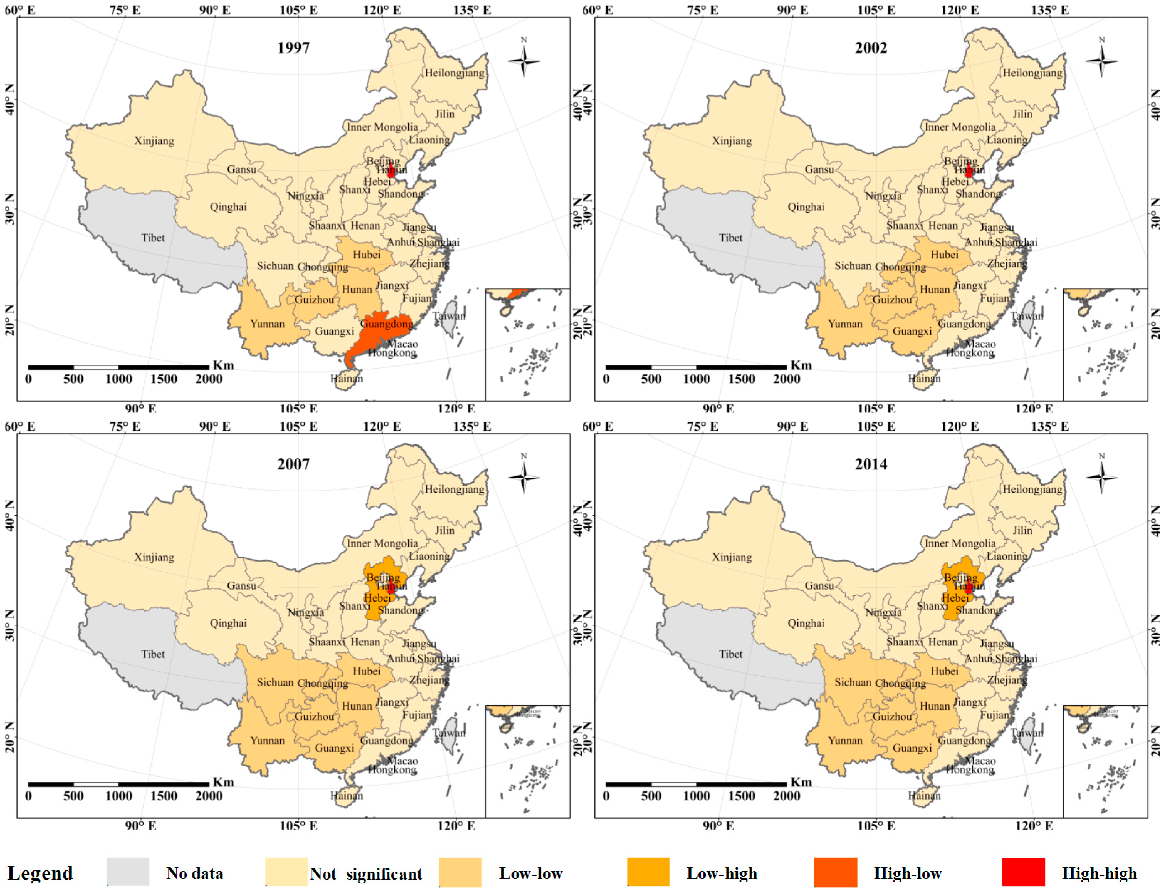
Figure 2 illustrates the temporal-spatial evolution of China’s PHCEs for each province in 1997, 2002, 2007, and 2014. The PHCEs of different provinces range from 0.60 t CO2/person in 1997 to 6.18 t CO2/person in 2014, differing by one order of magnitude. We classify the PHCEs of different provinces into five groups: lowest (less than 1.00 t CO2/person), low (1.01–2.00 t CO2/person), mid (2.01–3.00 t CO2/person), high (3.01–4.00 t CO2/person), and highest (more than 4 t CO2/person). In 1997, all provinces’ PHCEs were no more than 3.00 t CO2/person; thus they were classified into the lowest three groups. Of these, 16 provinces were in the lowest-level PHCEs, including northwest China, central China and southeast China. The 12 provinces with low-level PHCEs were concentrated in northeast China, the Qinghai-Tibet area, the Bohai Sea Region, and the Yangtze River Delta Economic Zone. By 2014, PHCEs in all provinces were more than 1.00 t CO2/person, constituting the top four groups. Only four provinces had low-level PHCEs in 2014, and these were among the poorest provinces: Gansu, Jiangxi, Guangxi, and Yunnan. The 16 provinces with mid-level PHCEs in 2014 were concentrated in the Qinghai-Tibet area, central China, and northern China. Six provinces that were either relatively wealthy (Guangdong, Fujian, Jiangsu) or had coal resources and a higher concentration of energy industries (Heilongjiang, Liaoning, and Inner Mongolia) had high-level PHCEs. Four of China’s wealthiest provinces, Beijing, Shanghai, Tianjin, and Zhejiang, had the highest-level PHCEs.
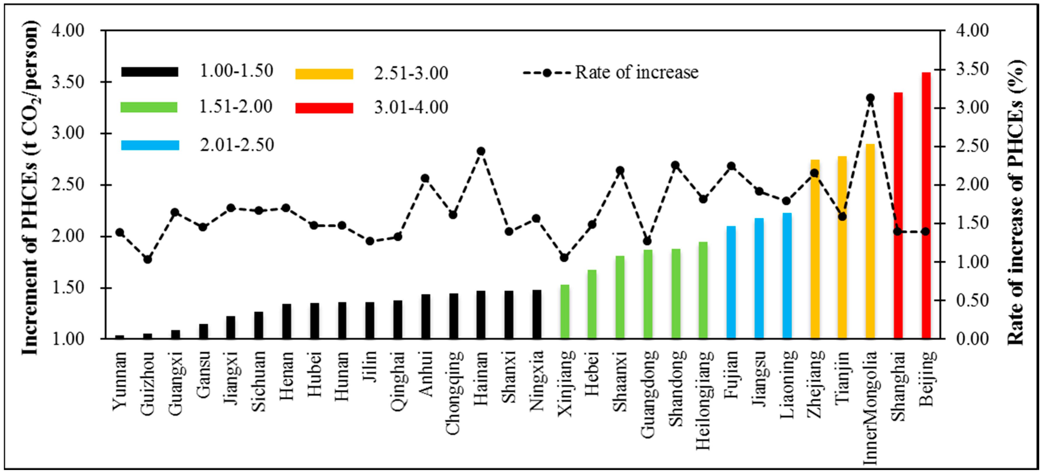
Figure 3 presents the increment and the increase rate of PHCEs from 1997 to 2014 for each province. All provinces’ PHCEs increased by more than 1.00 t CO2/person between 1997 and 2014. Twenty-two provinces had relatively low increases of PHCEs, from 1.00–2.00 t CO2/person. These provinces were relatively poor and were found in China’s southwest, northwest, and central regions. The two provinces with high increments of PHCEs, from 3.01 to 4.00 t CO2/person, were the rich provinces, Shanghai and Beijing. However, patterns in the rates of increase are somewhat different. Thirteen provinces had low rates of increase in PHCEs by one to two times. These can be divided into two groups; (1) relatively wealthy provinces, including Guangdong, Beijing, Shanghai, and other provinces with large PHCEs but with low rates of increase, and (2) relatively poor provinces with both low PHCEs and low rates of increase. Seven provinces had PHCEs more than double from 1997 to 2014. These included provinces with low PHCEs but high rates of increase (e.g., Anhui and Hainan) and provinces with both relatively high PHCEs and rates of increase (e.g., Zhejiang, Shandong, and Inner Mongolia).
3.2. Spatial Evolution Analysis of PHCEs in China
3.2.1. Results of Global Spatial Autocorrelation
While a regional pattern is clear from our descriptive analysis, we quantified this correlation using Moran’s I to evaluate the global spatial autocorrelation of PHCEs at the provincial level from 1997 to 2014. Table 2 shows that the Global Moran’s I of PHCEs in China for all years was above 0, indicating spatial clustering, and all are significant at a 95% confidence interval level based on the Z test. While the values of Moran’s I vary from year to year, over the study period, there was a general rising pattern from values in the low 0.2 range (0.22 in 1997) to the mid 0.3 range (0.37 in 2014). This pattern of increasing Moran’s I was matched by increasing statistical significance levels, from the 95% confidence range in 1997 to greater than 99% confidence by 2014. This indicates that there is significant and rising spatial autocorrelation for PHCEs in China.
3.2.2. Cluster and Outlier Analysis
We analyzed local spatial autocorrelation [31,32,33] using LISA for 1997, 2002, 2007, and 2014. Figure 4 reveals the characteristics of significant local spatial agglomeration in the distribution of PHCEs in China. Three significant patterns stand out. Firstly, the LL type of local spatial autocorrelation, which indicates provinces with low PHCEs that are also surrounded by provinces with low PHCEs, was present in central and southwest China for all years. This pattern can be seen in the provinces of Hubei, Hunan, Guizhou, and Yunnan for all years, as well as Sichuan, Chongqing, and Guangxi for all years except 1997 and 2002. Secondly, Guangdong, a manufacturing powerhouse located in the Southeast, has the HL pattern in 1997, indicating that Guangdong’s PHCEs are high whilst those of the surrounding provinces are low. However, Guangdong has no significant pattern in 2002, 2007, and 2014, indicating a convergence between Guangdong’s PHCEs and the surrounding provinces such as Fujian. Thirdly, in the Bohai region (Beijing, Tianjin, and Hebei), a notable shift occurred during the study period. Early in the study period (1997 and 2002), Beijing and Tianjin exhibited the HH pattern, indicating high PHCEs surrounded by provinces with high PHCEs. However, for 2007 and 2014, the adjacent Hebei province began to show a significant LH pattern, indicating low PHCEs surrounded by higher PHCEs. It is likely that this divergence during the course of the study period was driven by diverging PHCEs patterns within the Bohai region, with PHCEs rising rapidly in Beijing and Tianjin. Finally, it is worth noting that, in many regions of China, there were no significant patterns of local spatial autocorrelation, which is important to note in light of the significant patterns of global spatial autocorrelation. Most of northwest and northeastern China had no patterns of PCHEs spatial autocorrelation, nor did the Yangtze River Delta centered on Shanghai, Jiangsu, and Zhejiang. The latter example was particularly notable because the Yangtze River Delta, along with the Bohai region and Guangdong, was one of China’s most economically developed regions with relatively high PHCEs, yet, unlike the other two urban metropolises, the Yangtze Delta exhibited no patterns of local spatial autocorrelation in PHCEs.
3.2.3. Geographical Distribution of PHCEs in China
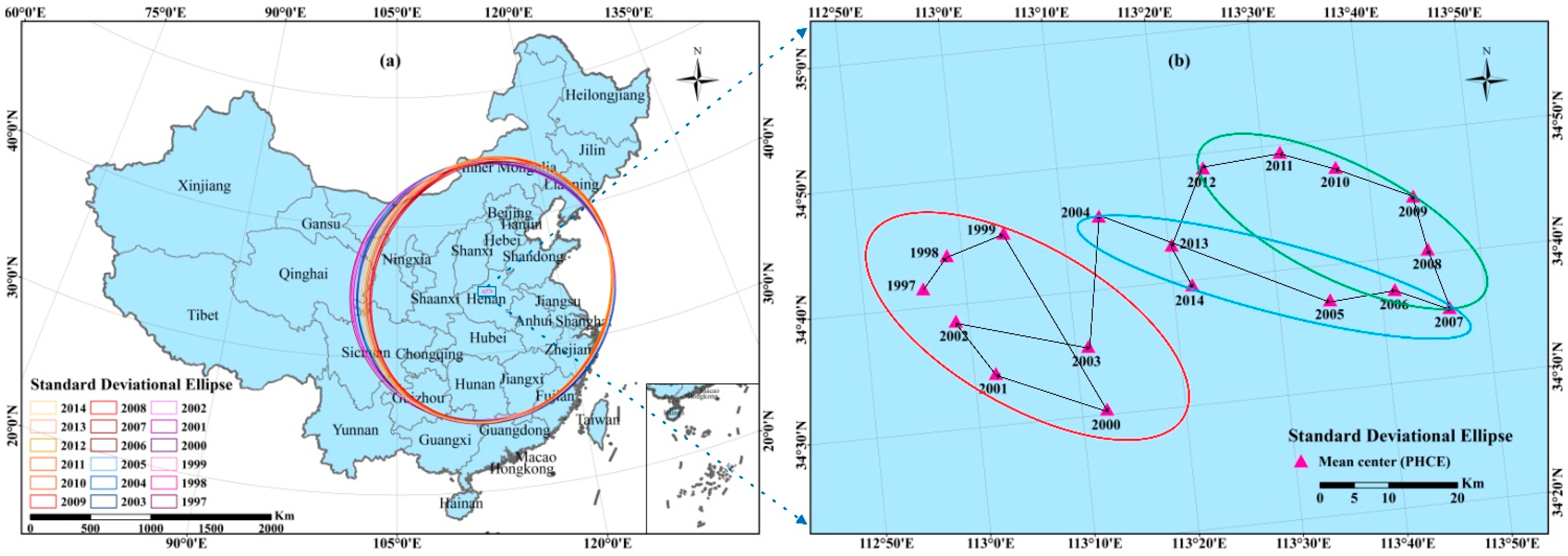
We used ArcGIS10.3 to analyze the gravity center of PHCEs in China following Zhao and Zhao [50]. The semi-major axis of the SDE represents the direction of distribution, whilst the short half axis of the SDE represents the range distribution. The greater the gap between the semi-major and short half axis, the more obvious the direction of distribution. If the length of the half shaft is completely equal to that of the semi-major axis, this means there is no direction characteristic [48]. As shown in Figure 5a, we can find that the gap between the semi-major axis and the short half axis of the SDE was not large in any year, which means that the gravity center offset of PHCEs in China is not obvious. Although there was little directional orientation to the location of PHCEs in China, important temporal trends did emerge. As shown in Figure 5b, the center of PHCEs in China during the study period was located between 34°30′–34°50′ N and 112°50′–113°50′ E. The movement of the SDE in PHCEs can be divided into three stages: firstly, from 1997 to 2003, it was located where the gravity center of PHCEs varied within a relatively small area; secondly, from 2004 to 2007, it was located where the gravity center of PHCEs moved approximately 60 km southeast; and thirdly, from 2007 to 2012, it was located where the center of PHCEs moved approximately 40 km to the northwest. As important as the individual patterns, it is worth noting that at all times during the study period, with the exception of 2003, 2004, 2013, and 2014, there was a relatively consistent pattern of movement in the center of gravity.
3.3. Spatial Panel Data Model of PHCEs in China
Based on the Hausman test, H2 was rejected while H1 was accepted, indicating that a variable intercept and constant coefficients model is most suitable [46]. Since the variables used in this work are co-integrated, the results for the four-type spatial panel data models (pooled regression model, spatial fixed effect, time period fixed effect, and spatial and time period fixed effect) are presented in Table 3. Comparing the estimators of R-squared, Adjusted R-squared, Log likelihood, Probability (F-statistic), and the Akaike info criterion in these four spatial panel data models, R-squared (0.97), Adjusted R-squared (0.96), and Log likelihood (200.47) are all higher and the Akaike info criterion (−0.55) is lower in the spatial and time period fixed effect than the other three models. Hence, the spatial and time period fixed effect model should be considered a fit model in this work. Based on the spatial and time period fixed effect model (Table 3), the parameter estimations of individual variable coefficients have important but slightly different influences on PHCEs in China.
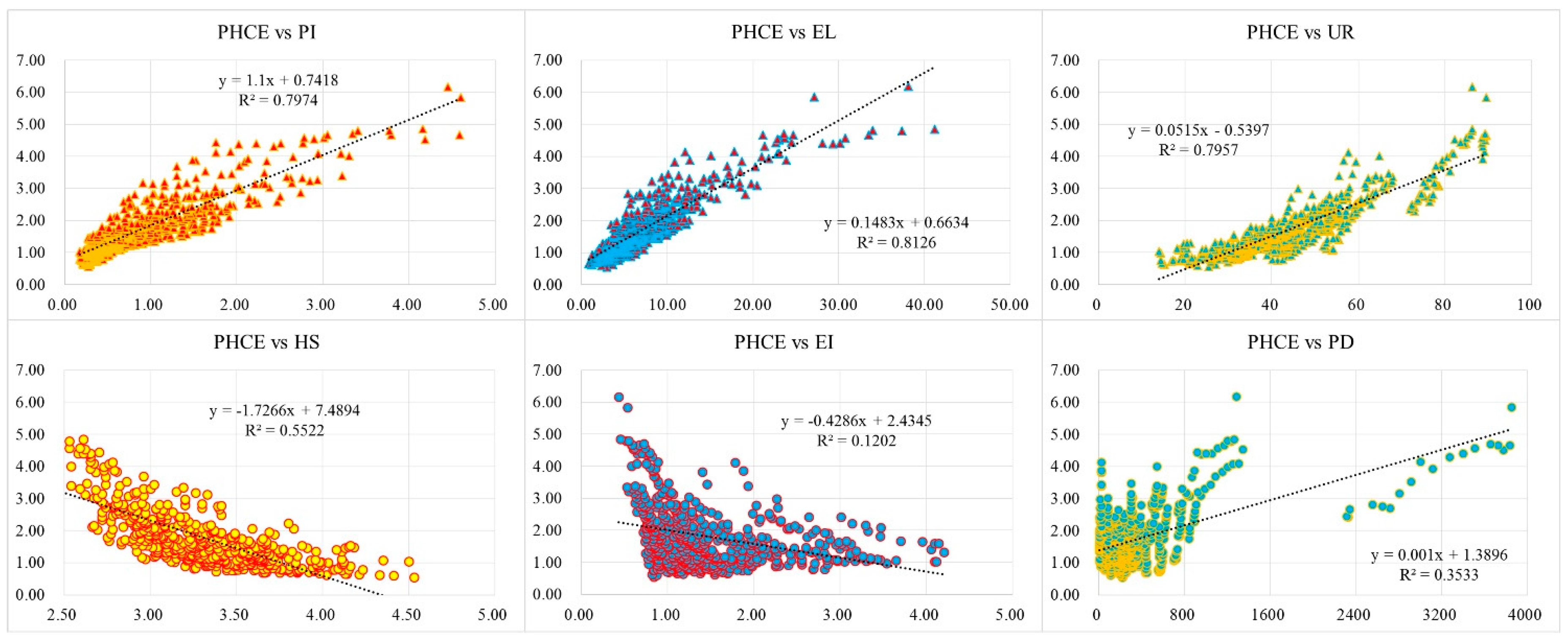
As shown in Figure 6, PI (Per capita income), EL (Education level), and UR (Urbanization) have a positive impact on PHCEs. HS (Household size) and EI (Energy intensity) have a negative impact on PHCEs. Based on the spatial panel data model, of the factors influencing PHCEs in China, PI (Per capita income) has a positive impact and the highest regression coefficient of 0.6990, followed by EL (Education level), and UR (Urbanization). As shown in Table 3, a 1% increase in PI, EL, and UR will result in 0.6990%, 0.0149%, and 0.0044% increases in PHCEs, respectively. HS (Household size) has a negative impact, with the highest regression coefficient of −0.0496, followed by PD (Population density). A 1% increase in HS and PD will result in 0.0496% and 0.0003% decreases in PHCEs, respectively. However, the coefficient of EI (Energy intensity) is not significant at the 5% level. Of the factors influencing PHCEs, we find that PI, EL, and UR have a positive influence, HS has a negative influence, and PD has a statistically significant negative influence, although very slight. The influence of EI on PHCEs, while negative, is not significant at the 5% level.
3.4. Discussions
Base on the movement of the SDE in PHCEs, the gravity center moves eastward first and then moves westward. There are two main reasons for this movement. First, economic development has a positive impact on PHCEs; meanwhile, the economic development in the East of China has been faster than in the West. Residents living in the East of China are relatively richer than those who live in the West of China. They have better living conditions, use more energy, and purchase more goods. This is why the gravity center moved eastward in the preliminary study period. Second, technology development has a substantial impact on PHCEs. The technological development in the East of China is also much faster than in the West. People that live in the East of China can get more information about renewable energy and clean energy, so they can enjoy the green energy welfare such as purchasing more energy-saving products. This is why the gravity center moved westward in the later study period.
After reviewing the spatial distribution and influencing factors of PHCEs in China, with an eye towards reducing PHCEs in China, we identify several trends.
First, PI has an important impact on PHCEs. The result that PI has a positive impact on PHCEs is similar with previous studies. Feng et al. [56] and Han et al. [26] showed that per capita income has a significant positive association with per capita CO2 emissions. As regions experience economic growth, household expenditure can be expected to rise, resulting in higher household consumption and associated emissions. PHCEs levels increase with both regional development and income level in this work.
Second, UR, and EL are also important factors that affect PHCEs in China in this analysis. The results in this work indicate that the rapid development of urbanization has increased household consumption and the related CO2 emissions. Zhang and Lin [57] pointed out that urbanization was positively related to energy consumption and the CO2 emissions in China based on a STIRPAT model and a spatial panel data model, respectively. Li et al. [58] revealed that there was a unidirectional causal relationship between urbanization and household carbon emissions. A 1% increase in urbanization may result in a 2.9% and 1.1% increase in direct and indirect household carbon emissions, respectively. Currently, China’s urbanization rate is projected to increase by 1.5% annually. Reducing PHCEs in the face of rapid urbanization presents a challenge and will require the decoupling of urbanization and PHCEs. With rapid urbanization in China, people’s lifestyles and habits have changed greatly. China’s urbanization rate is projected to increase, and this will further challenge the goal of carbon emissions reduction. Such challenges can be overcome through policy and changes in consumer behavior. Yang et al. [59] suggested that sustainable urban development should be highlighted and that enforcement of the law should be strengthened in ‘China’s new Environmental Protection Law’ [59]. Moreover, the advancement of technology can reduce carbon intensity and also save CO2 emissions. Therefore, technology should be improved to reduce environmental damage and develop more energy-saving products to cut carbon emissions.
The relationship between education and PHCEs has had mixed evaluations in the literature. Some have found that persons with higher education levels have higher emissions [60], while others claim that persons with higher education will help reduce carbon emissions [61,62]. There is ample grounding for both positions. The theory that higher education levels will reduce emissions is grounded in the belief that those with higher education levels are more aware of the adverse consequence of fossil fuel consumption and will adopt low carbon practices. The notion that higher education levels will lead to higher PHCEs is grounded in the belief that persons with higher education levels will purchase more modern products such as mobile phones, computers, and automobiles, thus resulting in more carbon emissions. Such consumer preference is also corroborated by the fact that those with higher education levels also have higher incomes. Our results indicate that the education level of household members positively, but only slightly, influences consumption attitudes and consumption habits, even when controlling for income. This influence is small in magnitude but significant at the 95% confidence level. We cannot, in this case, rule out the possibility of a latent variable, and the relationship between education and PHCEs is a likely venue for finer grained analysis.
Third, PHCEs decrease with increasing household size. This finding is similar to the findings of Qu et al. [8,9], who pointed out that PHCEs decreased as household size increased in northwest China. Large families, specifically extended families living together, presented a promising way to save energy and reduce CO2 emissions [8,9]. The same conclusion is found in Ireland [63]. When comparing per capita CO2 emissions between one-person households, two-person households, and any other household size, Lyons found that a larger household size will produce fewer per capita emissions than a lower household size.
The Chinese government has pledged to cut carbon intensity by 40% to 45% by 2020 from 2005 levels and to achieve peak CO2 emissions around 2030, which will result in more CO2 emissions from household consumption. These goals will be challenging in the face of rising income and urbanization levels, two factors that we have identified as influential for PHCEs. International comparisons point towards this difficulty, with CO2 emissions rising with increased income in Ireland [63] and China [21,26]. Thus, it is important to introduce policies to decouple increased household spending from rising emissions.
This could be accomplished through government policies that encourage consumers to use low-carbon products such as eco-labeling [64,65] and helping the producers of consumer goods to produce energy-saving products. However, it is ultimately consumers who must transition from luxurious to more frugal consumption activities [17] such as purchasing fuel-efficient cars and using more environmental-friendly home appliances. Consumers, as the drivers of markets for many energy-consuming items, should choose ‘green’ products to achieve a reduction in carbon emissions. Carbon labelled products should be considered important in this choosing process [64,65,66,67,68]. Increasing the ratio of renewable energy and clean energy in the total household energy usage in the future is also a very important measure to reduce CO2 from the household sector. These findings also highlight the importance of funding research into household emission mitigation measures.
Finally, although the connection between education level and emissions in general is ambiguous, education activities surrounding climate change should be publicized in schools and public places, especially in some rural areas, to explain individuals’ impact on climate change.
Although many findings highlighting the importance of this research on carbon reduction mitigation measures, a minor uncertainty in the results of accounting for PHCEs exists, owing to the inaccuracy or uncertainty of statistical data. First, heating usage in this study only includes the centralized heating usage in urban China. Centralized heating is only used in urban China so the centralized heating usage equals zero in rural China. Residents living in rural China mainly utilize small coal stoves (by using coal or gas) for heating in winter. Second, the emissions factors used to calculate CO2 emissions from the electricity sector (t CO2/MWh) for each province are based on data from 2010. The mix of electric generating sources changes constantly, which varies the carbon intensity of generation for two reasons; increasing the efficiency of fossil fuel (primarily coal) fired plans and changes in the mix of renewable and non-renewable sources. Data for electric emissions were selected for 2010 due to data being available for all provinces. Both of these sources of uncertainty could have a slight influence on our results.
Based on the aforementioned research results, the first way to reduce PHCEs is to narrow the difference of provincial PHCEs in China. Policy-makers should consider provincial differences when making policies impacting household emissions. China’s rapid development of urbanization has a great impact on PHCEs and thus policy-makers should; (1) consider the different urbanization ratios of different provinces and (2) seek ways to decouple urbanization from an increase in PHCEs. Provinces with higher PHCEs in China should have more responsibility to reduce emissions by taking on different responsibilities in a domestic form.
4. Conclusions
4.1. Conclusions
In this paper, we have investigated the spatial variations and determinants of per capita household CO2 emissions (PHCEs) in China. By analyzing the distributions of PHCEs in China, we examine the influencing factors of PHCEs using a spatial panel data model.
PHCEs at the provincial level grew rapidly from 1997 to 2014, with certain spatial patterns of variation enduring while others changed. The PHCEs of provinces ranged from 0.60 t CO2/person in 1997 to 6.18 t CO2/person in 2014, differing by one order of magnitude. Higher PHCE emitting regions are concentrated in eastern China, including Beijing, Shanghai, Zhejiang, and Tianjin. Lower PHCEs emitting regions are predominately in northwest and central China, including Guangxi, Anhui, Hainan, Qinghai, Gansu, and Ningxia. While individual provinces differed in their ranks in specific years, regional patterns of higher and lower PHCEs did not change during the study period. To lessen regional disparities and realize balanced development, regional compensation mechanisms, distinct development, and regional energy supply and demand must also be balanced.
To analyze the factors influencing PHCEs, geographically spatial dependence cannot be ignored. Based on the global Moran’s I index, we find a significant spatial autocorrelation of provincial PHCEs in China. We also reveal that the regions with high PHCEs tend to be adjacent to other regions with high PHCEs; regions with low PHCEs are also adjacent to each other. However, the gravity center offset of PHCEs in China is not obvious. The gravity center of PHCEs in China has moved between 34°30′–34°50′ N and 112°50′–113°50′ E, showing a distinct eastward movement between 2002 and 2007, with westward movement from 2007 to 2014.
We analyzed factors influencing PHCEs across Chinese provinces by using panel datasets. Our results show that PHCEs are increased by per capita income (PI), education level (EL), and urbanization (UR). A 1% increase in per capita income, education level, and urbanization will result in 0.6990%, 0.0149%, and 0.0044% increases in PHCEs, respectively. Household size (HS) has a negative impact with the highest regression coefficient of −0.0496, followed by population density (PD).
4.2. Policy Recommendations
Household CO2 emissions (HCEs) are increasing in China due to economic development and accelerated urbanization. Per capita income (PI) will keep growing in China, which will result in more CO2 emissions from household sector. Based on the results of spatial panel data model in this study, per capita income has a great impact on per capita household CO2 emissions (PHCEs). As regions experience different economic growth, policy makers should consider the impact of issues of increasing income and income disparity on PHCEs. It is urgent to introduce policies to decouple increased household spending from rising emissions.
Urbanization (UR) also has a positive impact on PHCEs in China and is likely to continue to do so in the future. One problem facing China is how to reduce carbon emissions in the face of rapid urbanization progress. It is necessary to guide residents to change their lifestyles and habits, yet there are positive signs in this regard. The proliferation of bike sharing services in China has increased the use of bike riding within close ranges, and the purchasing low-carbon and energy-saving products has increased. Education plays an important role in carbon reduction awareness. Our results reveal that an individual’s education level slightly influences their attitudes towards consumption and consumption habits, so it is very important to emphasize education in different regions. Education activities surrounding climate change should be publicized in schools and public places, especially in some rural areas, to promote environmental awareness to address climate change.
Although China’s PHCEs are much lower than those of developed countries, it is also important to prevent further increases of PHCEs. To achieve peak CO2 emissions around 2030, it is suggested to advance technology and establish a carbon emission trading system to reduce carbon intensity and reduce CO2 emissions from household consumption.
There are many factors affecting household CO2 emissions, including population, economic development, and demographic traits, all of which are identified by our spatial panel data model, which can give some suggestions for meaningful theoretical and policy implications. Measures for household carbon emission abatement should be proposed at the government and consumer levels. These findings also highlight the importance of funding research into household emission mitigation measures.
Acknowledgments
This work was founded by the National Key Research and Development Program of China (No. 2016YFA0602803) and the National Natural Sciences Foundation of China (No. 41371537), and we thank the editor and reviewers for their constructive comments and suggestions on the manuscript.
Author Contributions
Lina Liu, Jiansheng Qu, and Afton Clarke-Sather conceived and designed the experiments; Lina Liu, Jiansheng Qu, Afton Clarke-Sather, Tek Narayan Maraseni, and Jiaxing Pang performed the experiments; Lina Liu analyzed the data; and Lina Liu and Afton Clarke-Sather wrote the paper. All authors read and approved the final manuscript.
Conflicts of Interest
The authors declare no conflict of interest.
References
- IPCC (Intergovernmental Panel on Climate Change). IPCC Guidelines for National Greenhouse Gas Inventories; United Kingdom Meteorological Office: Bracknell, UK, 2006.
- Dietz, T.; Gardner, G.T.; Gilligan, J.; Stern, P.C.; Vandenbergh, M.P. Household actions can provide a behavioral wedge to rapidly reduce US carbon emissions. Proc. Natl. Acad. Sic. USA 2009, 106, 18452–18456. [Google Scholar] [CrossRef] [PubMed]
- Guan, D.B.; Peters, G.P.; Weber, C.L.; Hubacek, K. Journey to world top emitter: An analysis of the driving forces of China’s recent CO2 emissions surge. Geophys. Res. Lett. 2009, 36, 1–5. [Google Scholar] [CrossRef]
- Liu, L.C.; Wu, G.; Wang, J.N.; Wei, Y.M. China’s carbon emissions from urban and rural households during 1992–2007. J. Clean. Prod. 2011, 19, 1754–1762. [Google Scholar] [CrossRef]
- Zhu, Q.; Peng, X.Z.; Wu, K.Y. Calculation and decomposition of indirect carbon emissions from residential consumption in China based on the input-output model. Energy Policy 2012, 48, 618–626. [Google Scholar] [CrossRef]
- Tian, X.; Chang, M.; Lin, C.; Tanikawa, H. China’s carbon footprint: A regional perspective on the effect of transitions in consumption and production patterns. Appl. Energy 2014, 123, 19–28. [Google Scholar] [CrossRef]
- Zheng, S.Q.; Wang, R.; Glaeser, E.L.; Kahn, M.E. The greenness of China: Household carbon dioxide emissions and urban development. J. Econ. Geogr. 2011, 11, 761–792. [Google Scholar] [CrossRef]
- Qu, J.S.; Zeng, J.J.; Li, Y.; Wang, Q.; Maraseni, T.N.; Zhang, L.H.; Zhang, Z.Q.; Clarke-Sather, A. Household carbon dioxide emissions from peasants and herdsmen in northwestern arid-alpine regions, China. Energy Policy 2013, 57, 133–140. [Google Scholar] [CrossRef]
- Qu, J.S.; Zhang, Z.Q.; Zeng, J.J.; Li, Y.; Wang, Q.H.; Qiu, J.L.; Liu, L.N.; Dong, L.P.; Tang, X. Household carbon emission differences and their driving factors in north-western China. Chin. Sci. Bull. 2013, 58, 260–266. [Google Scholar] [CrossRef]
- Qu, J.S.; Maraseni, T.N.; Liu, L.N.; Zhang, Z.Q.; Yusaf, T. A comparison of household carbon emission patterns of urban and rural China over the 17 Year Period (1995–2011). Energies 2015, 8, 10537–10557. [Google Scholar] [CrossRef]
- Maraseni, T.N.; Qu, J.S.; Yue, B.; Zeng, J.J. Dynamism of household carbon emissions (HCEs) from rural and urban regions of northern and southern China. Environ. Sci. Pollut. Res. 2016, 23, 20553–20566. [Google Scholar] [CrossRef] [PubMed]
- Zhang, G.X.; Liu, M.X.; Gao, X.L. Dynamics characteristic analysis of indirect carbon emissions caused by Chinese urban and rural residential consumption based on time series Input-Output tables from 2002 to 2011. Math. Probl. Eng. 2014, 2014, 1–11. [Google Scholar] [CrossRef]
- Marks, R. Reducing carbon dioxide emissions from Australian energy. Sci. Total. Environ. 1991, 108, 111–121. [Google Scholar] [CrossRef]
- Stokes, D.; Lindsay, A.; Marinopoulos, J.; Treloar, A.; Wescott, G. Household carbon dioxide production in relation to the greenhouse effect. J. Environ. Manag. 1994, 40, 197–211. [Google Scholar] [CrossRef]
- Shorrock, L.D. Identifying the individual components of United Kingdom domestic sector carbon emission changes between 1990 and 2000. Energy Policy 2000, 28, 193–200. [Google Scholar] [CrossRef]
- Bin, S.; Dowlatabadi, H. Consumer lifestyle approach to US energy use and the related CO2 emissions. Energy Policy 2005, 33, 197–208. [Google Scholar] [CrossRef]
- Wei, Y.M.; Liu, L.C.; Fan, Y.; Wu, G. The impact of lifestyle on energy use and CO2 emission: An empirical analysis of China’s residents. Energy Policy 2007, 35, 247–257. [Google Scholar] [CrossRef]
- Kadian, R.; Dahiya, R.P.; Garg, H.P. Energy-related emissions and mitigation opportunities from the household sector in Delhi. Energy Policy 2007, 35, 6195–6211. [Google Scholar] [CrossRef]
- Weber, C.L.; Matthews, H.S. Quantifying the global and distributional aspects of American household carbon footprint. Ecol. Econ. 2008, 66, 379–391. [Google Scholar] [CrossRef]
- Liu, H.T.; Guo, J.; Qian, D.; Xi, Y.M. Comprehensive evaluation of household indirect energy consumption and impacts of alternative energy policies in China by input-output analysis. Energy Policy 2009, 37, 3194–3204. [Google Scholar] [CrossRef]
- Zha, D.L.; Zhou, D.Q.; Zhou, P. Driving forces of residential CO2 emissions in urban and rural China: An index decomposition analysis. Energy Policy 2010, 38, 3377–3383. [Google Scholar]
- Wang, Z.H.; Liu, W.; Yin, J.H. Driving forces of indirect carbon emissions from household consumption in China: An input-output decomposition analysis. Nat. Hazards 2015, 75, S257–272. [Google Scholar] [CrossRef]
- Zhu, Q.; Wei, T.Y. Household energy use and carbon emissions in China: A decomposition analysis. Environ. Policy. Gov. 2015, 25, 316–329. [Google Scholar] [CrossRef]
- Wang, Z.H.; Yang, L. Indirect carbon emissions in household consumption: Evidence from the urban and rural area in China. J. Clean. Prod. 2014, 78, 94–103. [Google Scholar] [CrossRef]
- Wang, Z.H.; Yin, F.C.; Zhang, Y.X.; Zhang, X. An empirical research on the influencing factors of regional CO2 emissions: Evidence from Beijing city, China. Appl. Energy 2012, 100, 277–284. [Google Scholar] [CrossRef]
- Han, L.Y.; Xu, X.K.; Han, L. Applying quantile regression and Shapley decomposition to analyzing the determinants of household embedded carbon emissions: Evidence from urban China. J. Clean. Prod. 2015, 103, 219–230. [Google Scholar] [CrossRef]
- Yuan, B.L.; Ren, S.G.; Chen, X.H. The effects of urbanization, consumption ratio and consumption structure on residential indirect CO2 emissions in China: A regional comparative analysis. Appl. Energy 2015, 140, 94–106. [Google Scholar] [CrossRef]
- Fan, J.; Wu, Y.R.; Guo, X.M.; Zhao, D.T.; Marinova, D. Regional disparity of embedded carbon footprint and its sources in China: A consumption perspective. Asia Pac. Bus. Rev. 2014, 21, 130–146. [Google Scholar] [CrossRef]
- Fan, J.L.; Liao, H.; Liang, Q.M.; Tatano, H.; Liu, C.F.; Wei, Y.M. Residential carbon emission evolutions in urban-rural divided China: An end-use and behavior analysis. Appl. Energy 2013, 101, 323–332. [Google Scholar] [CrossRef]
- Ala-Mantila, S.; Heinonen, J.; Junnila, S. Relationship between urbanization, direct and indirect greenhouse gas emissions, and expenditures: A multivariate analysis. Ecol. Econ. 2014, 104, 129–139. [Google Scholar] [CrossRef]
- Chuai, X.W.; Huang, X.J.; Wang, W.J.; Wen, J.Q.; Chen, Q.; Peng, J.W. Spatial econometric analysis of carbon emissions from energy consumption in China. J. Geogr. Sci. 2012, 22, 630–642. [Google Scholar] [CrossRef]
- Cheng, Y.Q.; Wang, Z.Y.; Ye, X.Y.; Wei, Y.H.D. Spatiotemporal dynamics of carbon intensity from energy consumption in China. J. Geogr. Sci. 2014, 24, 631–650. [Google Scholar] [CrossRef]
- Wang, S.J.; Fang, C.L.; Li, G.D. Spatiotemporal characteristics, determinants and scenario analysis of CO2 emissions in China using provincial panel data. PLoS ONE 2015, 10, e0138666. [Google Scholar] [CrossRef] [PubMed]
- Nejat, P.; Jomehzadeh, F.; Taheri, M.M.; Gohari, M.; Majid, M.Z.A. A global review of energy consumption, CO2 emissions and policy in the residential sector (with an overview of the top ten CO2 emitting countries). Renew. Sust. Energy Rev. 2015, 43, 843–862. [Google Scholar] [CrossRef]
- Dinda, S.; Coondoo, D. Income and emission: A panel data-based cointegration analysis. Ecol. Econ. 2006, 57, 167–181. [Google Scholar] [CrossRef]
- Narayan, P.K.; Narayan, S. Carbon dioxide emissions and economic growth: Panel data evidence from developing countries. Energy Policy 2010, 38, 661–666. [Google Scholar] [CrossRef]
- Niu, S.W.; Ding, Y.X.; Niu, Y.Z.; Li, Y.X.; Luo, G.H. Economic growth, energy conservation and emissions reduction: A comparative analysis based on panel data for 8 Asian-Pacific countries. Energy Policy 2011, 39, 2121–2131. [Google Scholar] [CrossRef]
- Ozcan, B. The nexus between carbon emissions, energy consumption and economic growth in Middle East countries: A panel data analysis. Energy Policy 2013, 62, 1138–1147. [Google Scholar] [CrossRef]
- Kais, S.; Sami, H. An econometric study of the impact of economic growth and energy use on carbon emissions: Panel data evidence from fifty eight countries. Renew. Sust. Energy Rev. 2016, 59, 1101–1110. [Google Scholar] [CrossRef]
- Hamit-Haggar, M. Greenhouse gas emissions, energy consumption and economic growth: A panel cointegration analysis from Canadian industrial sector perspective. Energy Econ. 2013, 34, 358–364. [Google Scholar] [CrossRef]
- Burnett, J.W.; Bergstrom, J.C.; Dorfman, J.H. A spatial panel data approach to estimating U.S. state-level energy emissions. Energy Econ. 2013, 40, 396–404. [Google Scholar] [CrossRef]
- Du, L.M.; Wei, C.; Cai, S.H. Economic development and carbon dioxide emissions in China: Provincial panel data analysis. China Econ. Rev. 2012, 23, 371–384. [Google Scholar] [CrossRef]
- Wang, S.J.; Fang, C.L.; Guan, X.L.; Pang, B.; Ma, H.T. Urbanization, energy consumption, and carbon dioxide emissions in China: A panel data analysis of China’s provinces. Appl. Energy 2014, 136, 738–749. [Google Scholar] [CrossRef]
- Wang, S.J.; Fang, C.L.; Wang, Y. Spatial variations of energy-related CO2 emissions in China and its influencing factors: An empirical analysis based on provincial panel data. Renew. Sustain. Energy Rev. 2016, 55, 505–515. [Google Scholar] [CrossRef]
- Hao, Y.; Chen, H.; Wei, Y.M.; Li, Y.M. The influence of climate change on CO2 (carbon dioxide) emissions: An empirical estimation based on Chinese provincial panel data. J. Clean. Prod. 2016, 131, 667–677. [Google Scholar] [CrossRef]
- Baltagi, B.H. Econometric Analysis of Panel Data; John Wiley & Sons Ltd.: Chichester, UK, 2005; pp. 215–231. Available online: http://max.book118.com/html/2015/0922/25967559.shtm (accessed on 19 July 2017).
- National Development and Reform Commission (NDRC). The First Ten Industries in Greenhouse Gas Emission Accounting Methods and Reporting Guidelines. Available online: http://bgt.ndrc.gov.cn/zcfb/201311/t20131101_568921.html (accessed on 19 July 2017).
- National Development and Reform Commission (NDRC). Factor for Provincial Power Grids in China. Available online: https://wenku.baidu.com/view/c2f4e1c3102de2bd960588f4.html (accessed on 19 July 2017).
- Anselin, L. Space and applied econometrics: Introduction. Reg. Sci. Urban. Econ. 1992, 22, 307–316. [Google Scholar] [CrossRef]
- Zhao, L.; Zhao, Z.Q. Projecting the spatial variation of economic based on the specific ellipses in China. Sci. Geogr. Sin. 2014, 34, 979–986. [Google Scholar]
- Lefever, D.W. Measuring geographic concentration by means of the standard deviational ellipse. Am. J. Sociol. 1926, 32, 89–94. [Google Scholar] [CrossRef]
- National Bureau of Statistics of China. China Energy Statistical Yearbook 1997–2014; China Statistics Press: Beijing, China, 1998–2015.
- National Bureau of Statistics of China. China Statistical Yearbook 1997–2014; China Statistics Press: Beijing, China, 1998–2015.
- National Bureau of Statistics of China. Input-Output Tables of China 1997, 2002, 2007, 2012; China Statistics Press: Beijing, China, 1999, 2007, 2009, 2015.
- National Bureau of Statistic of China. China Population Statistical Yearbook 1997–2006; China Population & Employment Statistical Yearbook 2007–2014; China Statistics Press: Beijing, China, 1998–2015.
- Feng, Z.H.; Zou, L.L.; Wei, Y.M. The impact of household consumption on energy use and CO2 emissions in China. Energy 2011, 36, 656–670. [Google Scholar] [CrossRef]
- Zhang, C.; Lin, Y. Panel estimation for urbanization, energy consumption and CO2 emissions: A regional analysis in China. Energy Policy 2012, 49, 488–498. [Google Scholar] [CrossRef]
- Li, Y.M.; Zhao, R.; Liu, T.S.; Zhao, J.F. Does urbanization lead to more direct and indirect household carbon dioxide emissions? Evidence from China during 1996–2012. J. Clean. Prod. 2015, 102, 103–114. [Google Scholar] [CrossRef]
- Yang, H.; Huang, X.; Thompson, J.R.; Flower, R.J. Enforcement key to China’s environment. Science 2015, 347, 834–835. [Google Scholar] [CrossRef] [PubMed]
- Liu, W.L.; Spaargaren, G.; Heerink, N.; Mol, A.P.J.; Wang, C. Energy consumption practices of rural households in north China: Basic characteristics and potential for low carbon development. Energy 2013, 55, 128–138. [Google Scholar] [CrossRef]
- Golley, J.; Meng, X. Income inequality and carbon dioxide emissions: The case of Chinese urban households. Energy Econ. 2012, 34, 1864–1872. [Google Scholar] [CrossRef]
- Dai, H.C.; Masui, T.; Matsuoka, Y.; Fujimori, S. The impacts of China’s household consumption expenditure patterns on energy demand and carbon emissions towards 2050. Energy 2012, 50, 736–750. [Google Scholar] [CrossRef]
- Lyons, S.; Pentecost, A.; Tol, R.S.J. Socioeconomic distribution of emissions and resource use in Ireland. J. Environ. Manag. 2012, 112, 186–198. [Google Scholar] [CrossRef] [PubMed]
- Zhao, R.; Deutz, P.; Neighbour, G.; McGuire, M. Carbon emissions intensity ratio: An indicator for an improved carbon labelling scheme. Environ. Res. Lett. 2012, 7, 2039–2049. [Google Scholar] [CrossRef]
- Zhao, R.; Zhou, X.; Jin, Q.; Wang, Y.T.; Liu, C.L. Enterprises’ compliance with government carbon reduction labelling policy using a system dynamics approach. J. Clean. Prod. 2016. Available online: https://doi.org/10.1016/j.jclepro.2016.04.096 (accessed on 15 Mary 2017). [CrossRef]
- Maraseni, T.N.; Qu, J.; Zeng, J. A comparison of trends and magnitudes of household carbon emissions between China, Canada and UK. Environ. Dev. 2015, 15, 103–119. [Google Scholar] [CrossRef]
- Maraseni, T.N.; Qu, J.; Zeng, J.; Liu, L. An analysis of magnitudes and trends of household carbon emissions in China between 1995 and 2011. Int. J. Environ. Res. 2016, 10, 179–192. [Google Scholar]
- Maraseni, T.N.; Xu, G. An analysis of Chinese perceptions on unilateral Clean Development Mechanism projects. Environ. Sci. Policy 2010, 14, 339–346. [Google Scholar] [CrossRef]
Figure 1.
Flowchart of the methodology for the spatial panel data model.

Figure 2.
The distribution of China’s total PHCEs in 1997, 2002, 2007, and 2014.

Figure 3.
Increment and rate of increase of PHCEs in China from 1997 to 2014.

Figure 4.
Spatial Moran’s I scatterplots of China’s PHCEs in 1997, 2002, 2007, and 2014.

Figure 5.
The geographical distribution trend of PHCEs in China (a); and the gravity center of PHCEs in China (b).
Figure 5.
The geographical distribution trend of PHCEs in China (a); and the gravity center of PHCEs in China (b).

Figure 6.
The relationship between PHCEs and the related influencing factors (Per capita income (PI), Education level (EL), Urbanization (UR), Household size (HS), Energy intensity (EI), and Population density (PD)).
Figure 6.
The relationship between PHCEs and the related influencing factors (Per capita income (PI), Education level (EL), Urbanization (UR), Household size (HS), Energy intensity (EI), and Population density (PD)).


Table 1.
The factors influencing per capita household CO2 emissions (PHCEs) in this work.
| Variables | Implication | Interpretation | Unit | Sources |
|---|---|---|---|---|
| PHCEs | Per capita household CO2 emissions | Total household CO2 emissions/total population | t CO2/person | Calculated by above formulas |
| PD | Per km2 areas population (Population density) | Administrative area/total population | person/km2 | China Statistical Yearbooks (1998–2015) |
| UR | Urbanization | The proportion of urban population | % | China Statistical Yearbooks (1998–2015) |
| HS | Household size | Average person in each household | Person/household | China Population Statistical Yearbooks (1998–2015) |
| EL | Education level | The proportion of college educated people and/or higher educational level students in the population | % | China Statistical Yearbooks (1998–2015) |
| PI | Per capita income | Total income/total population | 104RMB/person | China Statistical Yearbooks (1998–2015) |
| EI | Energy intensity | Total Energy usage/Total GDP | t ce/104RMB | China Statistical Yearbooks (1998–2015) |
Table 2.
Changes of the Global Moran’s I of PHCEs in China (1997–2014).
| Year | I | Z | P |
|---|---|---|---|
| 1997 | 0.22 | 1.98 | 0.04 |
| 1998 | 0.24 | 2.12 | 0.03 |
| 1999 | 0.26 | 2.12 | 0.04 |
| 2000 | 0.28 | 2.27 | 0.03 |
| 2001 | 0.27 | 2.07 | 0.04 |
| 2002 | 0.28 | 2.29 | 0.03 |
| 2003 | 0.29 | 2.58 | 0.02 |
| 2004 | 0.25 | 2.12 | 0.03 |
| 2005 | 0.29 | 2.34 | 0.02 |
| 2006 | 0.32 | 2.62 | 0.02 |
| 2007 | 0.32 | 2.45 | 0.02 |
| 2008 | 0.34 | 2.51 | 0.02 |
| 2009 | 0.35 | 2.65 | 0.02 |
| 2010 | 0.34 | 2.54 | 0.01 |
| 2011 | 0.34 | 2.56 | 0.01 |
| 2012 | 0.33 | 2.53 | 0.02 |
| 2013 | 0.37 | 2.78 | 0.01 |
| 2014 | 0.37 | 2.81 | 0.01 |
Table 3.
Estimation of influencing factors on PHCEs in by the spatial panel data model.
| Panel Data Model | Pooled Regression Model | Spatial Fixed Effect | Time Period Fixed Effect | Spatial & Time Period Fixed Effect |
|---|---|---|---|---|
| C | 1.7756 *** | 0.4784 *** | 1.2156 *** | |
| PD | 0.0001 *** | 0.0001 | 0.0000 * | 0.0003 *** |
| UR | 0.0214 *** | 0.0091 *** | 0.0182 *** | 0.0044 ** |
| HS | 0.0559 *** | 0.3087 *** | 0.1903 *** | 0.0496 ** |
| EL | 0.0421 *** | 0.0199 ** | 0.0413 *** | 0.0149 ** |
| PI | 0.4989 *** | 0.5921 *** | 0.6557 *** | 0.6990 *** |
| EI | 0.1241 ** | 0.0237 * | 0.1263 *** | 0.0697 * |
| R-squared | 0.92 | 0.96 | 0.93 | 0.97 |
| Adjusted R-squared | 0.92 | 0.96 | 0.93 | 0.97 |
| Log likelihood | −39.44 | 131.46 | 5.96 | 200.47 |
| Prob(F-statistic) | 0.00 | 0.00 | 0.00 | 0.00 |
| Akaike info criterion | 0.19 | −0.35 | 0.07 | −0.55 |
Notes: * Significant at the 10% level; ** Significant at the 5% level; *** Significant at the 1% level.
© 2017 by the authors. Licensee MDPI, Basel, Switzerland. This article is an open access article distributed under the terms and conditions of the Creative Commons Attribution (CC BY) license (http://creativecommons.org/licenses/by/4.0/).
Share and Cite
MDPI and ACS Style
Liu, L.; Qu, J.; Clarke-Sather, A.; Maraseni, T.N.; Pang, J. Spatial Variations and Determinants of Per Capita Household CO2 Emissions (PHCEs) in China. Sustainability 2017, 9, 1277. https://doi.org/10.3390/su9071277
AMA Style
Liu L, Qu J, Clarke-Sather A, Maraseni TN, Pang J. Spatial Variations and Determinants of Per Capita Household CO2 Emissions (PHCEs) in China. Sustainability. 2017; 9(7):1277. https://doi.org/10.3390/su9071277
Chicago/Turabian StyleLiu, Lina, Jiansheng Qu, Afton Clarke-Sather, Tek Narayan Maraseni, and Jiaxing Pang. 2017. "Spatial Variations and Determinants of Per Capita Household CO2 Emissions (PHCEs) in China" Sustainability 9, no. 7: 1277. https://doi.org/10.3390/su9071277
Note that from the first issue of 2016, this journal uses article numbers instead of page numbers. See further details here.