Statistical Building Energy Model from Data Collection, Place-Based Assessment to Sustainable Scenarios for the City of Milan

Mutani, Guglielmina; Alehasin, Maryam; Usta, Yasemin; Fiermonte, Francesco; Mariano, Angelo

doi:10.3390/su152014921

Open AccessArticle

Statistical Building Energy Model from Data Collection, Place-Based Assessment to Sustainable Scenarios for the City of Milan

¹

Department of Energy, Politecnico di Torino, 10129 Turin, Italy

²

Urban Sustainability & Security Laboratory for Social Challenges, S3+Lab, Politecnico di Torino, 10125 Turin, Italy

³

Energy Technologies and Renewable Sources Department, ICT Division, ENEA (Agenzia Nazionale per le Nuove Tecnologie, L’energia e lo Sviluppo Economico Sostenibile—National Agency for New Technologies, Energy and Sustainable Economic Development), 70125 Bari, Italy

^*

Author to whom correspondence should be addressed.

Sustainability 2023, 15(20), 14921; https://doi.org/10.3390/su152014921

Submission received: 8 September 2023 / Revised: 1 October 2023 / Accepted: 13 October 2023 / Published: 16 October 2023

(This article belongs to the Special Issue Building Energy and Structural Deep Renovation: Analysis, System and Approach)

Abstract

:

Building energy modeling plays an important role in analyzing the energy efficiency of the existing building stock, helping in enhancing it by testing possible retrofit scenarios. This work presents an urban scale and place-based approach that utilizes energy performance certificates to develop a statistical energy model. The objective is to describe the energy modeling methodology for evaluating the energy performance of residential buildings in Milan; in addition, a comprehensive reference dataset for input data from available open databases in Italy is provided—a critical step in assessing energy consumption and production at territorial scale. The study employs open-source software QGIS 3.28.8 to model and calculate various energy-related variables for the prediction of space heating, domestic hot water consumptions, and potential solar production. By analyzing demand/supply profiles, the research aims to increase energy self-consumption and self-sufficiency in the urban context using solar technologies. The presented methodology is validated by comparing simulation results with measured data, achieving a Mean Absolute Percentage Error (MAPE) of 5.2%, which is acceptable, especially considering city-scale modeling. The analysis sheds light on key parameters affecting building energy consumption/production, such as type of user, volume, surface-to-volume ratio, construction period, systems’ efficiency, solar exposition and roof area. Additionally, this assessment attempts to evaluate the spatial distribution of energy-use and production within urban environments, contributing to the planning and realization of smart cities.

Keywords:

Urban Building Energy Modeling; statistical model; urban scale; residential buildings; energy performance certificates (EPCs); energy efficiency; renewable energy sources; solar technologies; space heating; domestic hot water; electrical consumption; QGIS; self-sufficiency; self-consumption

1. Introduction

The compelling growth of cities and the consequent higher energy consumption in urban territories underlines the importance of taking actions to mitigate climate changes associated with high concentration of energy-use and low renewable energy sources in these critical areas. The significance of cities’ capacity to respond and recover from energy disturbances and shocks is emphasized by the concept of urban resilience. Urban areas should be prepared for future challenges and ensure long-term sustainability by adapting and transforming their systems to overcome interruptions or limitations on the use of energy [1].

The United Nation (UN) defined 17 Sustainable Development Goals (SDGs), which encourage actions for a more sustainable future, with clean energy production and lower consumption, especially in cities and communities. The UN-Energy plan of action is committed to reaching a 100% increase in renewables capacity globally, to meet 100% renewables-based power targets established in 100 countries, and to increase the annual rate of energy efficiency from 0.8 to 3% in at least 50 countries across the world [2]. The new energy challenges are availability, accessibility, acceptability and convenience to ensure an overall global resilience of energy systems with benefits for all. It is important to integrate these four challenges with planning, preparation, absorption, recovery, and adaptation to consider the complex links between stakeholders, governance, social and economic factors, resources, infrastructure, and individual behavior [3]. The widespread actions that lead to energy sustainability and resilience of urban spaces are: energy efficiency, renewable energy, and the smart grid. Certainly, these actions can be facilitated by a framework of governance, policies and incentives that need to be explored for each specific case study and the modeling proposed in this work helps in this direction.

The building sector accounts for an important quota of energy consumption, making this sector play an essential role in the application of sustainable urban strategies. Therefore, for the building sector, it is crucial to understand and optimize the energy consumption profiles of the different users, variables affecting energy consumption, the available energy resources and greenhouse gas emissions (GHG). In Europe, residential buildings have the highest energy consumption, and the most widely used fuel is natural gas, followed by electricity and renewables, respectively (Figure 1); for residential buildings, space heating accounts for 63.6% among the other energy services, showing the importance of meeting energy production and consumption profiles, especially during the heating season. In Italy, the problem is more complicated by the great dependence on foreign countries, mainly for both natural gas and electricity. Thus, the seasonal hourly profiles of energy consumption, and the renewable production and self-sufficiency potential, with their spatial distribution within a city, are important indicators for modeling the energy–environmental–economic–social performance of a smart energy system in order to boost the post-carbon transition.

Energy consumption significantly depends on several variables related to many aspects. The more important energy-related variables that affect the energy performance of buildings are: climate conditions, geometric and typological features of the buildings (volume, surface-to-volume ratio S/V, period of construction, etc.), urban context typology (buildings’ density, urban canyons’ height-to-width ratio H/W, etc.), and population’s socio–economic characteristics (people’s age, number of family members, maintenance level of buildings, etc.) [5]. For example, the S/V ratio represents how much the building is non-compact and demonstrates the importance of building form in controlling the heat flow to/from the outdoor environment; detached houses have higher energy consumption compared to condominiums since the S/V ratio is higher. In addition, the urban density and aspect ratio H/W of urban canyons influence the solar exposition, the radiant flux between buildings and to the sky, and local climate conditions, with consequences for energy consumption.

McKeen and Fung illustrated significant changes in space heating and cooling consumption for various residential building typologies, cities, aspect ratios, building orientations, shapes, and construction periods [5]. Generally, older buildings exhibited higher energy consumption due to poor thermal insulation and low technological system efficiencies. However, between 1961 and 1980, energy usage increased, primarily due to the use of low-performance construction materials during the post-World War II economic popular housing boom and because of the higher window-to-wall ratio. Duran et al. analyzed an energy model to enhance modeling precision using open-data sources at an urban scale [6]. The study’s results emphasize the importance of having detailed data for a reliable energy performance analysis of buildings at an urban scale. It specifically highlights the challenges in modeling certain population characteristics, such as presence and behavior, as these are complex and uncertain variables that can influence building energy usage. One solution was to use synthetic population data and average values for people density per floor area at a block of buildings scale. To achieve a higher resolution, it might be essential to simulate various presence profiles. According to Malhotra et al., simulating multiple presence profiles can provide a more comprehensive understanding of the complex and uncertain variables influencing energy usage in buildings, leading to more accurate energy modeling at an urban scale [7]. Using building characteristic features becomes beneficial when processing data for multiple buildings on an urban scale while employing data-driven modeling [8].

This work aims to present a place-based assessment for the city of Milan to understand the actual energy performance and the energy efficiency potential of the existing building stock. The statistical Urban Building Energy Modeling (UBEM) applied for the city of Milan can help to evaluate the role of buildings in reducing energy consumption and the share of renewable energy sources (RES) from building to district-urban level. The choice of a statistical model is due to the possibility of accessing the Energy Performance Certificates (EPCs) database [9] and to the lack of consumption data at building scale. This energy modeling makes it possible to evaluate the consumption of the buildings before and after the energy retrofit interventions and therefore considering the interventions that are actually carried out taking into account the existing historical, environmental and economic constraints. The use of the free tool, Quantum Geographic Information System (QGIS), is fundamental for geo-localizing information, and assessing the spatial distribution of energy-related variables and consumption data. QGIS consents to exploit all databases and information with different scales, allowing an accurate place-based modeling for each building at urban scale.

2. The City of Milan

Milan is one of the most important and populated cities in Italy. According to the National Institute of Statistics ISTAT [10], in recent years, the population is quite stable with about 1,350,000 inhabitants. The blocks of residential buildings number about 43,000 (i.e., 66%) with 700,000 dwellings mainly built in 1919–1960 (51%). Most residential buildings (70%) have more than five apartments with about two components per family.

Milan has a temperate climate with cold winters and hot humid summers. It is a typical mega-city with the urban heat island effect. In recent decades, Milan has registered an average annual air temperature of 14.3 °C, 2274 heating degree days at 20 °C and 81 cooling degree days at 26 °C [11].

Table 1 shows the average monthly air temperature and solar irradiation; it can be observed that the heating season starts in the second half of October and ends in mid-April; the cooling season is concentrated in the summer months of June, July and August.

In 2008, Milan decided to join the Covenant of Mayors’ initiative to reduce greenhouse gas (GHG) emissions and energy consumption, and to increase the share of energy produced from renewable sources [12]. Referring to the year 2005, the GHG emissions were 5.67 tonCO₂/capita (with final energy consumption of 18.97 MWh/capita) and, because of various energy and climate actions, in 2020 fell to 3.4 tonCO₂/capita (i.e., −40%).

Due to the many constraints on the use of renewable energy technologies in a high-density city, photovoltaic technology is the main used RES in the city of Milan with an installed power of only 24.6 MW.

Milan is monitoring the use of energy and GHG emissions [13,14,15] and has joined international initiatives to reduce them, such C40 Cities Climate network, Urban Agenda Partnership on Air Quality, the revision of the Sustainable Energy and Climate Action Plane (within the Covenant of Mayors), Resilient Cities Network, European initiative EIT, Climate KIC and KIC Mobility initiative [16]. To reach its energy and climate targets, Milan is one of the Italian cities that participate in the 100-climate neutral and smart cities by 2030 and Reinventing Cities programs. These initiatives are opportunities that cannot be missed to start processes for a sustainable development of the city, an improvement of the quality of life and a commitment to achieve the highest level of decarbonization. Furthermore, in the building code regulations, Milan sets the minimum environmental sustainability requirements to be achieved, and environmental or economic compensation actions.

3. Materials and Methods

In this work, the description of the urban context is based on a place-based approach considering all the features that describe both buildings and their surrounding space. Together with the characteristics of the buildings, the most influential urban variables are urban building density, dimensions of urban canyons, sky view factor, main orientation of streets, properties of urban surfaces, and presence of green areas and water.

The novelty of this work is in providing a detailed approach for UBEMs with a complete set of databases and geodatabases. Table 2 provides the information to calculate all energy-related variables useful to build energy consumption models at an urban scale; geo-localize energy production systems and plants; assess the availability of renewable energy sources (RES) that can be used to supply clean energy in each Italian territory. Moreover, the QGIS methodology is explained in detail by providing the pre-processing and modeling steps necessary for a place-based approach. The objective is to describe a replicable methodology and modeling that can be used for all urban contexts and climate conditions.

The QGIS place-based approach is well described in some results of the Cities on Power project [17] and other more recent research [18,19]. In these works, the authors described the place-based approach to buildings’ energy consumption and production through renewable energy sources using free databases and an open-source tool (QGIS). QGIS is not only a tool to visualize, represent and map data but also to overlap, analyze, manage, create information, and for modeling. Certainly, it is widely used because of its possibility to spatialize data and results, providing a better comprehension of energy matters.

Urban Building Energy Modeling can be divided into four phases represented in the flowchart of Figure 2: pre-modeling, modeling, calibration and representation of the results. These phases are described in detail in the following sections.

Section 3.1 describes the pre-modeling, which is one of the most important phases of Urban Building Energy Modeling with data collection and pre-processing analyses. The input data are processed and associated with the spatial or territorial unit of the model (i.e., dwelling, building, neighborhood, district, municipal area) to build a database as complete as possible. The spatial unit used in this work corresponds to the building, and by knowing the physical phenomenon of the heat exchanges between buildings and the external environment, all the variables that could influence the energy modeling are calculated and added to the geo-database.

The energy consumption which is used to define the modeling approach (bottom-up or top-down) is collected from the Energy Performance Certificates (EPCs) database. In Section 3.1.1, the EPC database of the buildings is described, and this led to the decision to use the bottom-up approach and statistical modeling (considering the energy performance index of each dwelling). Since the higher quota of energy consumption in Milan is attributed to the civil sector and mainly to residential buildings, this model considers residential buildings, with their main energy-use for space heating (H) and domestic hot water (DHW). Electricity data (E) for the consumption of inhabitants in 2018 and 2022 were used with the hourly profile provide by ARERA for the Province of Milan [20,21].

Then, in the modeling phase (Section 3.2), the GIS-based methodology is described in detail. The geo-database is used to extract further energy-related variables from building geometry and to create the 3D model of the city of Milan. Then, indicators and variables related to energy consumption are identified and analyzed in order to assess the actual scenario with a spatial distribution of the consumption through the urban area. Future scenarios can be foreseen assuming the adoption of some energy efficiency measures and greater use of available renewable energy sources.

Finally, Section 3.3 describes in detail the process of using EPCs for the statistical model, which is the core of this work, finding the variables that affect energy-use and highlighting the challenges behind gathering the correct information about building size, period of construction, and inhabitants.

The main field of application of this model will be the identification of the most effective energy policy for sustainable development of the specific high-density city of Milan.

3.1. Data Collection

For the evaluation of the energy consumption, production, and possible future production in the Italian territory, some examples of input data at a national-local level have been reported in Table 2. This table is subdivided by databases, tools, and platforms for energy-consumption variables, technologies, and energy-related data, with information about energy costs too. These databases/tools can be used to analyze actual and future energy consumption and production, evaluate the available renewable sources and optimize energy supply and demand in a future post-carbon scenario. Table 2 can allow access, through a place-based approach, to the availability of renewable energy resources to cover energy demand at each point of the Italian territory. This table is very important because most of the information is open-access and therefore already available. Furthermore, the place-based analysis, which can be performed with this information, also concerns all the constraints that exist on the territory, making energy modeling more realistic.

The databases used for the statistical energy-use model for each building of the city of Milan (i.e., with 74,936 blocks of residential buildings) are the following: the municipal technical map of the city with the description of building characteristics, the map of census sections-districts and municipal boundaries, the digital terrain model (DTM, every 10 m), the 2011 ISTAT census database on population and buildings, the Regional Registry for Thermal Plants and Systems, mainly for space heating and hot water production, and the Atlaimpianti web-tool for actual renewable energy systems. The Energy Performance Certificates (EPCs) database at building scale [9] and the Covenant of Mayors’ data at municipal scale [12] were used to calibrate and validate the energy model for residential buildings in the city of Milan.

3.1.1. Energy Performance Certificates Database

The Energy Performance Certificates (EPCs) database was used to obtain information about the energy-use and primary energy consumption, energy classes, and energy efficiency levels of the buildings [9]. Energy performance certificates (EPCs) of 277,121 were collected, released from October 2015 till May 2022. These EPCs were georeferenced to apply the place-based approach and only 251,320 EPCs had a correct and complete address. Then, EPCs were analyzed and extracted to include only residential buildings according to the Italian Decree 412/1993: E.1 (1) permanent residences.

This first selection reduced the number of EPCs from 251,320 to 209,969.

The big database of EPCs allows a bottom-up approach from building to urban scale. For each EPC, the characteristics of the residential building were collected (e.g., geometry, typology and technological system characteristics) including the period of construction. Together with building geometry, the period of construction is very important because over the years the buildings have been constructed with different types of envelopes, levels of thermal isolation, window-to-wall ratio and systems efficiencies. Some important laws (and corresponding dates) are useful for assessing the energy efficiency level of buildings in Italy: Law 373/1976, Law 10/1991, Decree Lgs. 192/2005 and Law 90/2013 as subsequently amended and supplemented. In Milan, residential buildings were mainly built as follows: 27% before 1945, 25% in 1946–1960, 30% in 1961–1976, and only 13% after 1992 (after the first Italian laws on energy saving in buildings). In Figure 3, it is possible to observe the period of construction of the buildings in the central historical districts of the City of Milan; almost all buildings were built before 1960 (i.e., before Law 373/1976); in Milan, this percentage is 65%. Older buildings are concentrated in the center and in old settlements near transport infrastructure and industries; newer buildings are in the peripheral areas and in new districts.

Using the ISTAT database, the number and characteristics of inhabitants and families were collected for each census section; then these data were processed as per volume data and assigned to each residential building. Figure 4 illustrates the number of families in residential buildings resulting from the number of families per census section and the percentage of gross heated volume per building. The majority of buildings in the center host between 1 to 26 families per building, which suggests that there are few historical condominiums, or that only a portion of the buildings is residential.

The ISTAT database was also used to calculate the real heated volume considering the number of empty apartments and other energy-related characteristics of buildings (e.g., maintenance level and property conditions).

Table 3 shows the percentage of EPCs by period of construction and energy class. An improvement in energy classes for newer buildings can be observed, especially after 1991. Until 1980, most of the buildings are in class G, then in the 1980s a higher percentage moves into class F and after 1991 into class D; the more recent buildings are in class A3. Overall, most of the buildings belong to the most energy-intensive classes F and G with 56% (E, F, G 75%); considering the percentage of buildings by the period of construction, 52% of buildings were built before 1960 and 82% before 1976 (before the first Italian Law on energy savings in buildings), hence they need retrofit interventions. The energy classes, efficiency level, and consumption, mainly for space heating and domestic hot water, of the EPCs’ database are investigated to define an urban building energy model.

3.2. Pre-Processing and Geographical Database Creation

In the pre-processing phase, the geometrical variables that strongly influence the energy consumption were calculated, such as the heated gross volume, heat loss surfaces and the net heated floor area. For the calculation of the surface-to-volume ratio S/V, a special procedure in QGIS software was necessary to consider the shared walls between adjacent buildings and the presence of unheated volumes. In general, space heating consumption increases with S/V.

Afterwards, according to the surface-to-volume ratio and the number of floors, different categories of buildings were identified: detached, terrace (maximum three floors), row, and tower buildings. In Figure 5, the gross volume of residential buildings is represented. This is one of the main energy-related variables for space heating and it was used to calculate the net volume, and the net heated volume and area. The calculation of the net heated area is very important because is used to calculate both the dimension of the building and its energy performance index. This map shows the volume of merged blocks of buildings, so it is notable to have a quite high-volume range in the legend. For more precise modeling, the building shapefile should be more detailed, representing single polygons for each building (for Milan these data are not available).

In Figure 6, the typology of residential buildings is represented and classified. The type of building was determined as a function of the surface-to-volume ratio (S/V) that represents the non-compactness of buildings. Considering buildings with equal volume V, the higher is S (the heat loss surface area), the higher will be the energy consumption for space heating. It can be observed that there are mainly towers or row houses; only in districts 2, 7, 8 and 9 is the percentage of detached houses about 22%, 20%, 16%, and 23%, respectively. Districts 8 and 9, on the North-East side of the city, are the most populated. For this work, given the large amount of data, the city of Milan has been divided into nine districts to manage and represent the spatial distribution of buildings and energy consumption.

The 3D model of the city is represented in Figure 7 with the altitude of the built environment in meters a.s.l. To describe the 3D built environment of the city of Milan, a Digital Surface Model (DSM) was created. Generally, this analysis starts from a Lidar flight which allows the building of an accurate 3D model of the city. In the absence of a Lidar flight, the orography of the territory with the Digital Terrain Model (DTM) was merged with the 3D model of the buildings, considering the area and height of the buildings. It is important to mention that the DSM created for this work is not as accurate as a real DSM, because it does not consider the exact shape of buildings, therefore presenting all buildings as flat roofed.

3.3. Statistical Modeling of Buildings’ Energy Consumption

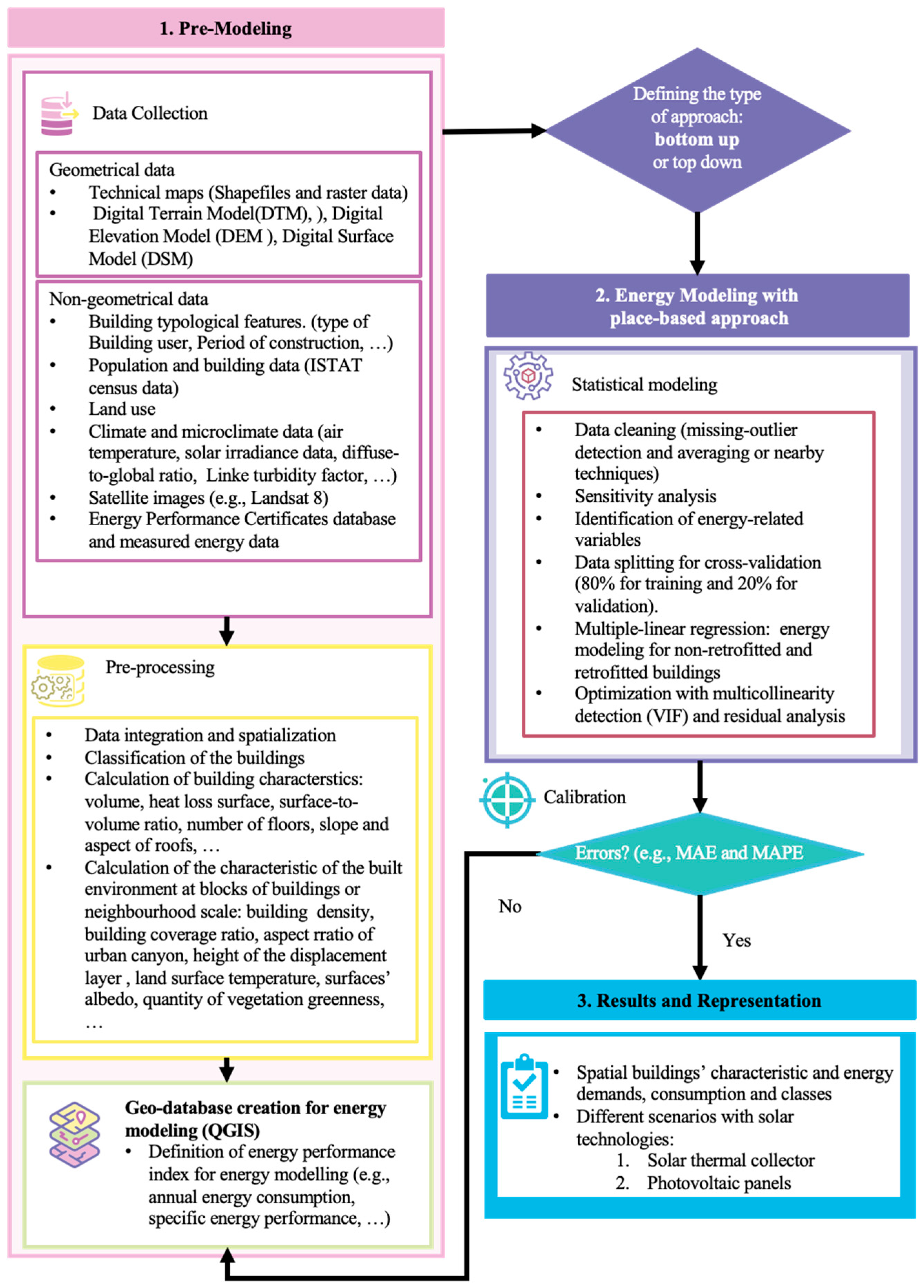
The goal of the statistical energy modeling was to evaluate the energy performance index (EP) of residential buildings for the city of Milan from the EPCs’ database. In particular, the specific energy demand for space heating (EP_H) and the overall primary energy index (EP_gl,nren) of the buildings were considered.

The statistical assessment can be synthesized in the steps below:

(1): data collection from EPCs’ database, technical maps and ISTAT data;
(2): pre-processing phase to calculate and add other variables that could influence the energy consumption;
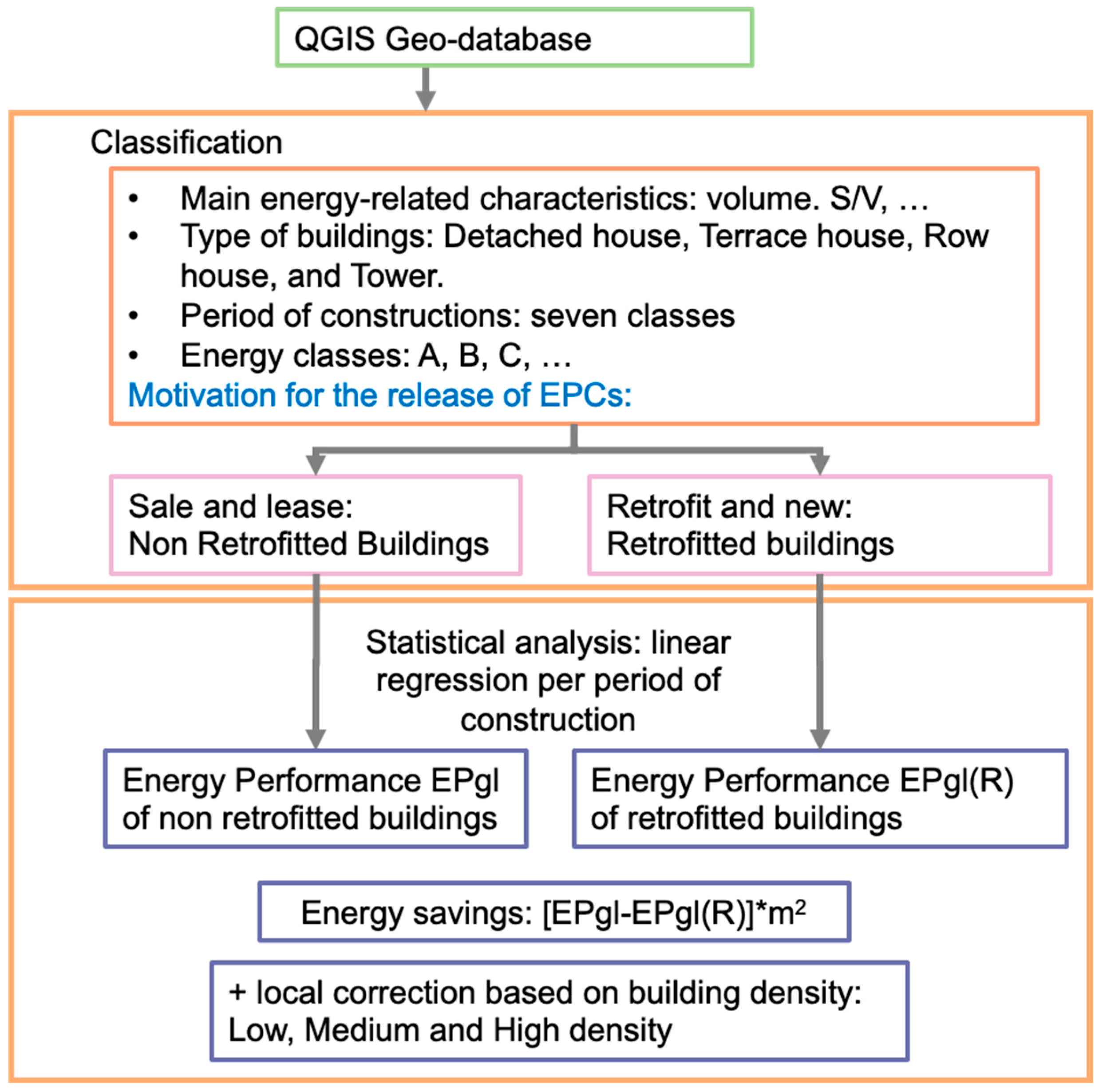
(3): the database of EPCs was subdivided into two datasets of non-retrofitted and retrofitted buildings considering the motivation of the release of the EPCs;
(4): evaluation of the more energy-related variables with Pearson’s correlation;
(5): definition of subsets of consumption data considering the more energy-related variables; for each subset, the frequency distribution of consumption data was verified with the Kolmogorov–Smirnov and/or Chi-squared tests;
(6): identification and exclusion of outliers from EPCs’ database together with the null data;
(7): formulation of the multilinear regression for the evaluation of the energy performance of non-retrofitted and retrofitted buildings;
(8): multicollinearity and residual analysis;
(9): definitive multilinear regression models.

Figure 8 represents the elaboration steps applied to the available EPCs, which are part of the preprocessing phase of the presented energy modeling. The initial step is to classify the buildings according to some energy-related characteristics considering their geometric attributes, which in turn will be used to define additional parameters (e.g., S/V ratio is used to define building typology). The ISTAT database is also used to classify the buildings according to their period of construction. The energy performance of the buildings can be calculated based on the seven classes of period of construction and the S/V ratio. The motivation for releasing EPCs is to categorize the data based on the new, retrofitted, sale, and lease of the buildings. Then, statistical analysis was applied to calculate the linear regression for energy performance and S/V using EPCs data.

From the early stages of the analysis, the EPCs’ database was divided to train and then test the model with a respective percentage of data equal to 80% and 20%.

Using the EPCs’ database, the energy consumption of the non-retrofitted building stock and the retrofitted one was calculated considering standard climate conditions and the average use of residential buildings according to the Energy Performance Certification Standards. Comparing the resulting models, applied to the city of Milan, the percentage of energy savings that can be achieved is evaluated by taking into account all the actual energy, environmental, economic and social constraints.

One important limit of energy modeling at urban scale is the availability of data for all the buildings in Milan, which are:

from the technical map of the city of Milan: the building use, footprint area, height or number of floors, gross volume, net heated surface, surface-to-volume ratio S/V, period of construction;
from the National Institute of Statistics ISTAT for population and buildings: the number of inhabitants and families, age, nationality, working level, buildings’ property, level of maintenance, occupation profile, period of construction class.

Description of Alternative Machine Learning Models

There are several machine learning (ML) models that can be applied in the energy sector in order to analyze, monitor and manage energy consumption, each of them depending on the typical task that they need to accomplish.

In the supervised domain, where typical problems are energy consumption prediction, fault detection and load forecasting, the main algorithms are based on Random Forest, an ensemble learning technique made of simple decision trees; on Gradient Boosting, an evolution of ensemble techniques made of weak learners trying to reduce the distance between obtained output and ground truth; on Support Vector Machines, an attempt to find the best boundary that separates the data into different classes, by maximizing the margin, which is the distance between the boundary and the closest data points from each class; or on Neural Networks, a family of machine learning algorithms that are particularly well-suited to problems that involve high-dimensional, complex data. When in a supervised setting, data are sequential as in time series forecasting, Recurrent Neural Networks, e.g., Long Short-Term Memory cells, usually take place. A typical example of a supervised task is a regression model, which can be trained on a dataset of historical energy usage data from a building to learn the relationship between different factors (such as weather conditions, occupancy levels, and building features) and the building’s energy consumption. The trained model can then be used to make predictions about the building’s future energy usage based on new data inputs.

In the unsupervised domain, where the task is to identify patterns in energy consumption data and detect anomalies, or facilitate data fusion and integration, the techniques are based on, for example: k-means clustering, used to group similar data points together into clusters; self-organizing maps, used to map high-dimensional data onto a lower-dimensional grid of neurons; and auto-encoders, that map the input data to a lower-dimensional, bottleneck feature representation.

In the reinforcement learning domain, where an agent must learn how to act in a sequential environment to maximize some reward, optimization problems usually arise and ML algorithms are based on Monte Carlo or temporal difference techniques, a mathematical framework for decision-making problems where the future is uncertain, that tries to identify the optimal policy that allows the agent to choose the best action to perform in the environment. For example, the scheduling of renewable energy generation, such as wind or solar power, can be adjusted through these algorithms to maximize the amount of energy generated while minimizing the cost.

In Figure 9, typical tasks in the energy sectors tackled by machine learning approaches are shown, and a review is discussed in a recent paper [22]; however, it is worth noting that the field is rapidly evolving, and new techniques may emerge as better options for specific problems.

Predicting energy consumption at the urban/territorial scale with data-driven models typically involves collecting data on a variety of factors that can impact a city’s energy usage, such as the age and size of buildings, the type of heating and cooling systems used, the weather, and the population density. This data is then processed using machine learning algorithms to train a model that can make predictions about a city’s future energy consumption or about other cities, based on data collected from an analogous distribution. This model can be used to help city planners and policymakers make decisions about how to reduce energy usage and improve energy efficiency in the city or in a territory.

4. Results and Discussion

4.1. Energy Performance Certificates (EPC) Analysis

To simulate the energy performance (EP_gl,nren) of the existing building stock, and therefore compare the energy efficiency level before and after retrofit measures, the data for the residential buildings of Milan have been processed to obtain all energy-related characteristics. To evaluate the energy efficiency level of the buildings, it was necessary to identify the typological and geometric characteristics that influence their energy-use. Buildings were classified into seven classes by the period of construction: before 1930, 1930–1945, 1946–1960, 1961–1976, 1977–1992, 1993–2006, and after 2006. To simplify the analysis, the buildings built before 1945 were grouped, as the characteristics of these buildings are similar, with no thermal insulation, brick walls and slabs, low glazing ratio, and low energy efficiency systems; they constitute over 64% of all buildings in Italy, as per ISTAT’s report in 2001 [10].

Table 4 illustrates the energy classes of residential buildings, global energy performance (EP_gl,nren) and motivation for release. Buildings without data on EP_gl,nren and with “empty” or “other” motivations for release were neglected; then the dataset of EPCs is reduced from 209,969 to 189,756. It has been assumed that the non-retrofitted buildings are those identified by the energy performance certificate as for sale or lease. Retrofitted buildings are only 8.8% and new buildings are 4.8%. Comparing these data, it can be observed that after retrofit interventions the energy performance of buildings is improved from class G to class F; it must be remembered that these interventions are the actual ones, and the most frequent is the replacement of windows, with a fairly low improvement in energy performance. A total of 65% of new buildings are in class A. Because of the low number of retrofitted interventions, especially for recent periods of construction, these two datasets (retrofitted and new buildings) have been merged in the “retrofitted” database.

Figure 10 represents the energy classes of residential buildings before (a) and after (b) retrofit interventions. Before retrofit measures, the prevailing classes are F and G, while after retrofitting, this becomes D, E and F. A total of 25% of buildings after retrofit interventions belong to classes A, B and C, and only 7% before retrofitting interventions.

For cross-validation, the EPCs’ database was divided into two datasets: 80% as training set and 20% as testing set. This data splitting is necessary to ensure the evaluation of the energy model’s performance, using 80% of the data, allowing it to learn and capture patterns from this larger portion. Once the model is built and trained, it can be tested using the remaining 20% of the data, which served as the validation step.

The analysis of the collected EPCs, which are registered from October 2015 until May 2020, gives an important insight into the effectiveness of retrofit interventions in global energy saving. The number of apartments renewed is 17,738 for the whole registered period with an average heated surface area of 388,665 m²/year.

Figure 11a illustrates the sum of heated surfaces for the different years and (b) the cumulative energy savings after retrofit interventions; energy savings are almost constant. This last analysis uses the retrofitted surfaces and the difference between the average values of energy performance indexes before and after retrofit interventions (see Figure 10).

4.2. GIS-Based Energy Modeling and Sensitivity Analysis

In order to enhance the model’s representation of Milan’s energy performance, the global, non-retrofitted and retrofitted datasets were selected for conducting of sensitivity analyses. The main information used comes from: EPC database, ISTAT database with the characteristics of population and buildings, the technical map of Milan, and income data by district in 2020.

The Pearson’s correlation was applied to two energy performances indexes (EP): the space–heating energy performance need (EP_H,nd) and the global primary energy performance, not considering the use of renewable sources (EP_gl,nren); the average and median values of EPs are indicated in Table 5. Comparing the values of EP, with the retrofitted buildings there are potential energy savings of 43–39%.

The main energy-related variables with the strongest Pearson’s correlations to energy performance are presented in Table 6. The higher Pearson’s correlation with energy performance, the more the energy-related variables: period of construction, S/V ratio and the year of systems’ installation. Potential energy performance after retrofit interventions and the CO₂ emissions, which are directly influenced and therefore not independent of the EPs, were not considered in the modeling; also, the year of the systems’ installation was not taken into consideration because this information is not available at an urban scale.

From the dataset of non-retrofitted buildings, the average potential energy performance is about 110 kWh/m²/y with a payback time of 5–15 years depending on the type of intervention; this is probably due to multiple urban constrains in this high-density urban environment.

It can be observed that there is a negative correlation between energy performance and period of construction because, for newer buildings the energy performance index EP decreases. The same applies for the year of systems’ installation: newer installation means higher efficiency of the systems and therefore a lower energy performance index EP. There is a positive correlation with the surface-to-volume ratio S/V because higher S/V means lower compactness and therefore higher heat loss surfaces of buildings, with a higher energy performance index EP. In this work, period of construction and S/V ratio of buildings are used for modeling their EP at an urban scale because the year of installation of the systems is unknown for all buildings in Milan. As is possible to observe, the socio–economic data were lowly correlated to energy performance and neglected for this analysis (only the main energy-related examples are reported).

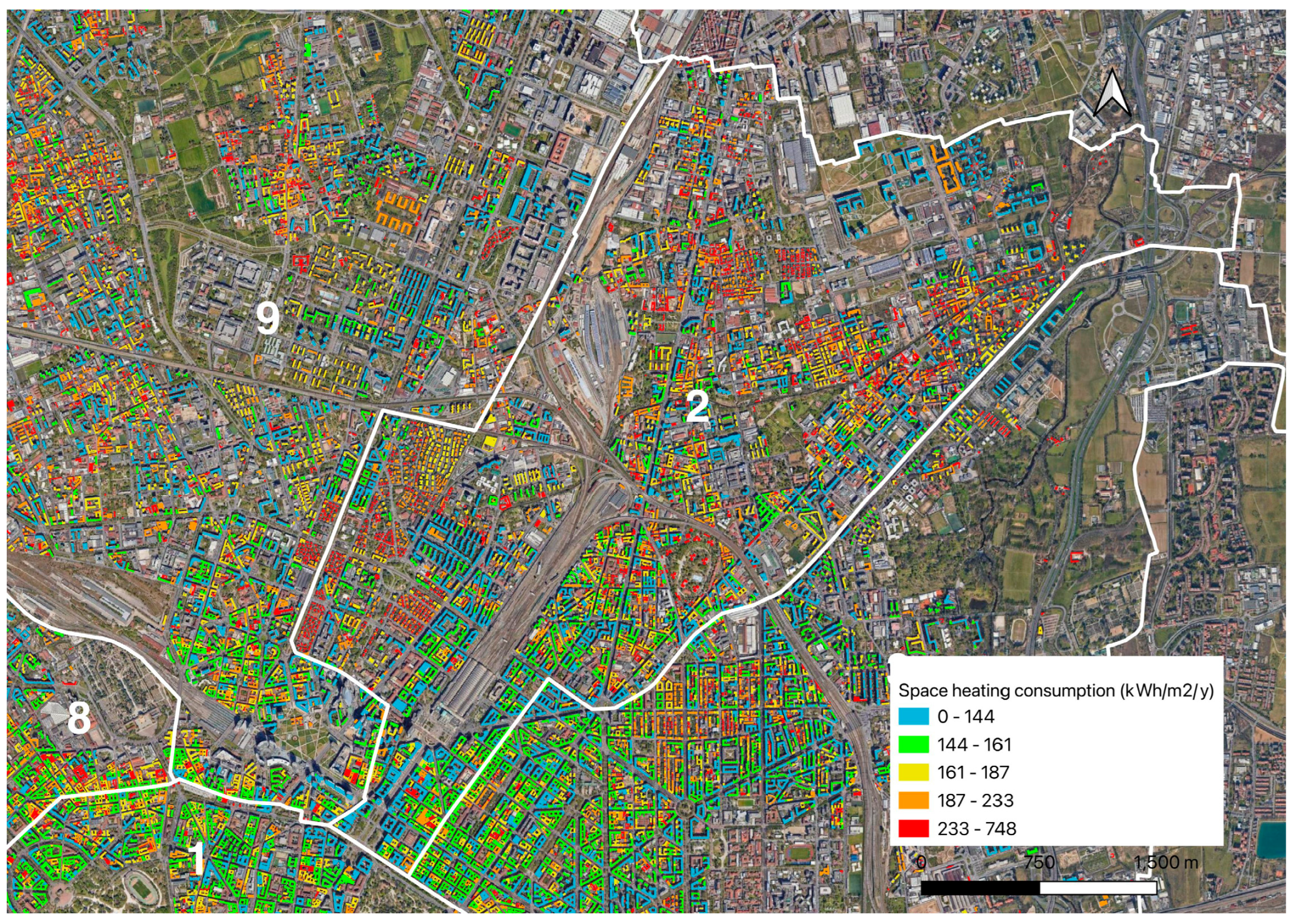
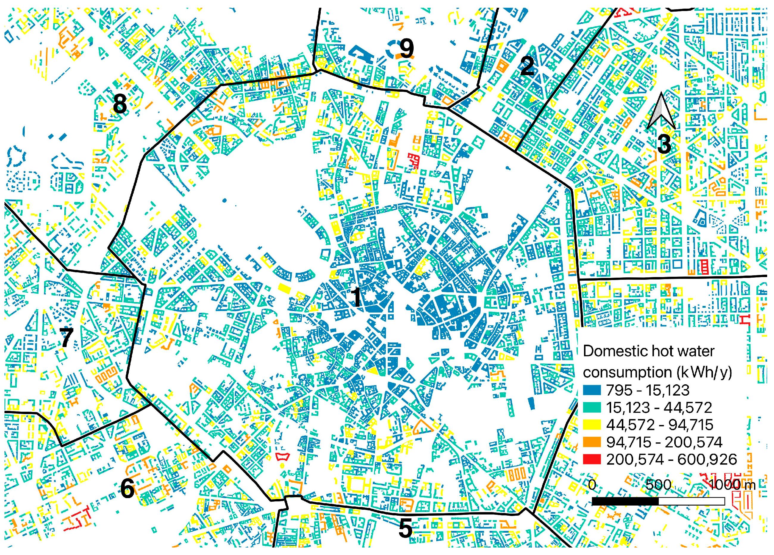
4.3. Statistical Energy Consumption Model

The choice of statistical modeling in this work is due to its powerful role in assessing big databases with a simple methodology and extracting meaningful insights and patterns from large amounts of data. These models offer the advantage of systematically analyzing information, identifying trends, and making informed predictions. It is also possible to define easily homogenous classes of buildings based on their characteristics by utilizing various classification techniques and frequency distribution; these techniques were used to group buildings with similar attributes into distinct categories but also to identify outliers.

This statistical energy modeling with a place-based approach can extract valuable data from different sources in order to analyze the current energy consumption model with more input data and then define future energy savings and production scenarios.

Using the QGIS software, the results of the models for energy consumption and solar thermal and electrical energy production are presented in the sections below for residential buildings. The annual energy performance for space heating H and DHW before and after retrofit interventions was computed and compared with the amount of energy that can be produced through solar technologies for the city of Milan. Similarly, the electricity demand was compared with the electricity produced by photovoltaic modules. All solar technologies are roof-integrated to reduce the visual impact of solar panels, but it is very important to boost this resource, especially in high-density cities where almost no other RES is available.

Considering the period of construction and the surface-to-volume ratio S/V (the main energy-related variables), the EPCs were grouped considering only these two variables. Then, the normal distribution of the EP_gl,nren was calculated for each homogeneous group and verified by the Kolmogorov–Smirnov and/or Chi-squared tests. This phase allows the checking of outliers or null values of S/V, period of construction and, using the normal distribution, of EP_gl,nren, obtaining a database of 121,967 EPCs.

Table 7 shows the number of buildings per homogeneous group without outliers that were used for the statistical modeling. For the period of construction, the ISTAT classes were used because this range is available for the city of Milan and will make the model more applicable. It is possible to observe that, for recent periods of construction, the low number of buildings can affect the result, especially for retrofitted buildings.

Based on this classification, for each homogeneous group of buildings, the average energy performance index EP_gl,nren was computed. This average EP_gl,nren was used in the linear regression model depending on the S/V, for each period of construction.

The building density influencing the solar gains, the radiant fluxes to the surrounding objects and the sky and local climate conditions were also taken into account. This allows a more detailed place-based approach. In Figure 12, QGIS software was used to evaluate the density of buildings, based on census sections, and categorized it into three classes: low, medium, and high, considering respectively 60%, 30%, and 10% of areas.

Figure 13 represents the resulting linear regression of the energy performance index EP_gl,nren by the period of construction and S/V, before (a) and after (b) retrofit interventions. These linear regressions take into consideration Milan’s climate conditions, type of building stock, energy services (which are mainly space heating H 100% and domestic hot water DHW 99.8%; only 37.7% have cooling systems) and the main retrofit interventions made in Milan due to technical, historical, environmental, and socio–economic constraints (only 8.8% for the total EPC). Higher S/V ratio values result in higher primary energy consumption, and the EP_gl,nren after retrofit intervention decreased by about 40%, showing the importance of enhancing the efficiency of the existing building stock.

To obtain the energy consumption, the EP_gl,nren values were multiplied by the net heated floor area of each building and then divided by the primary energy coefficient of the fuel (mainly natural gas 83.1%, electricity 6.4% and district heating 7.6%).

Figure 14 illustrates how the energy performance (EP) is influenced by the density in the city of Milan, explaining local climate conditions in urban canyons, solar exposition and radiative heat flow to the nearby buildings and the sky. Each point shows the average EP by type of building density and period of construction; the missing points are not significant due to a too low number of buildings. As it is possible to observe, building density and energy performance are inversely correlated (at census section scale); in general, low building density means 5–12% higher consumption considering, respectively, medium- and high-density contexts.

Therefore, in this model, the energy performance depends on the surface-to-volume ratio S/V and the period of construction but is corrected by the building density.

Figure 15 indicates the process of calculating the energy performance for residential buildings using QGIS. After adding the vector layer of the Technical Map of the city of Milan to QGIS, first it is important to select only the residential buildings and calculate the footprint area, perimeter, volume and number of floors of each building. It is important to consider only heated buildings. Buildings with a footprint area lower than 50 m² and a height lower that 3.3 m were excluded. All characteristics of the buildings can be checked in the attribute table of the buildings’ shape file. The calculation of new variables (geometrical, but not only) can be obtained by creating a new column using the “field calculator”.

For high-density cities, a quite complicated step in this analysis is the calculation of the surface-to-volume ratio S/V (point 6 in 13). Indeed, the common surfaces between adjacent buildings should be subtracted by the heat loss surface S and the unheated volumes, inside the buildings, should be subtracted by the gross volume V. To identify the common surfaces a geo-package was created from the building shapefile using the DB manager and a query was written (see Appendix A) to measure the border length (L_COND) between each adjacent building. The second step is to create a narrow buffer to the perimeter of each building, which will help in finding the lower/common height of the intersecting buildings; with the field calculator, it is possible to identify the lower buildings by the positive or negative sign of the height difference HDIFF between the adjacent buildings. Knowing the height of the two buildings, the lowest will be selected and multiplied by L_COND (obtained in the first step from the virtual layer) to calculate the common area between two buildings. Then, the unheated gross volumes inside the buildings can be evaluated by typical coefficients for each type of building to correct the real volume V_real. After this automatic calculation of S/V_real, it is possible to acquire many related geometric variables (e.g., useful heated surface, window surface, vertical wall surfaces, etc.) that are helpful inputs for possible retrofit scenarios.

Energy consumption data can be computed from the modeling application knowing the energy performance index EP_gl,nren. This place-based approach using QGIS allows evaluation of EP_gl,nren and consequently energy consumption (mainly for space heating and domestic hot water) for each building in a city using the field calculator tool.

As mentioned before, only the space heating and domestic hot water services were considered in the primary energy performance index EP_gl,nren because they are the more frequent; moreover, natural gas fuel was assumed for the same reason:

EP_gl,nren = EP_H,nren + EP_DHW,nren = (EC_H,nren + EC_DHW,nren). f_p,nren/m²

(1)

where:

-: EP_nren is the primary energy performance index in kWh/m²/year considering non-renewable sources for space heating (H) and domestic hot water (DHW);
-: EC is the energy consumption (or delivered energy) in kWh/year;
-: f_p,nren is the conversion factor of delivered energy into primary energy (for natural gas, this is 1.05);
-: m² is the net heated area of a building.

Then, the Energy Consumption for DHW EC_DHW,nren of each building was calculated considering a volume of 50 L/person/day, a temperature gradient of 30 °C (with an average water temperature from the aqueduct of 15 °C) and an average system efficiency of 0.8. Knowing the energy consumption for domestic hot water (i.e., about 796 kWh/inh/year), the energy consumption for space heating was evaluated.

This place-based methodology has been used to define the energy model and apply it to all the buildings in the city of Milan knowing the number of inhabitants per building. The QGIS tool enables us to enhance the accuracy of the model with an iterative procedure to reduce its errors; this calibration procedure modified input data manually. This phase could be improved by automatizing it through decision tree algorithms with Machine Learning (ML).

The model was calibrated and then validated by comparing the application of the statistical model (in Figure 13 and Figure 14) with the global primary energy from the EPCs’ database and the energy consumption for space heating and domestic hot water in all of the city of Milan during 2017: 12,200 GWh [23].

In Figure 16, the annual consumption for space heating is represented. The consumption was calculated from the model represented in Figure 13 and Figure 14 supposing that natural gas is supplied. With this model, energy consumption depends on the shape of the building (with the surface-to-volume S/V), the period of construction and the building density. The empty spaces in the central district 1 in Milan indicate that no residential buildings are present. The calculation of space heating considered only the net heated areas inside each residential building, excluding unheated spaces, like empty apartments, stairwells, hallways, and entrance halls.

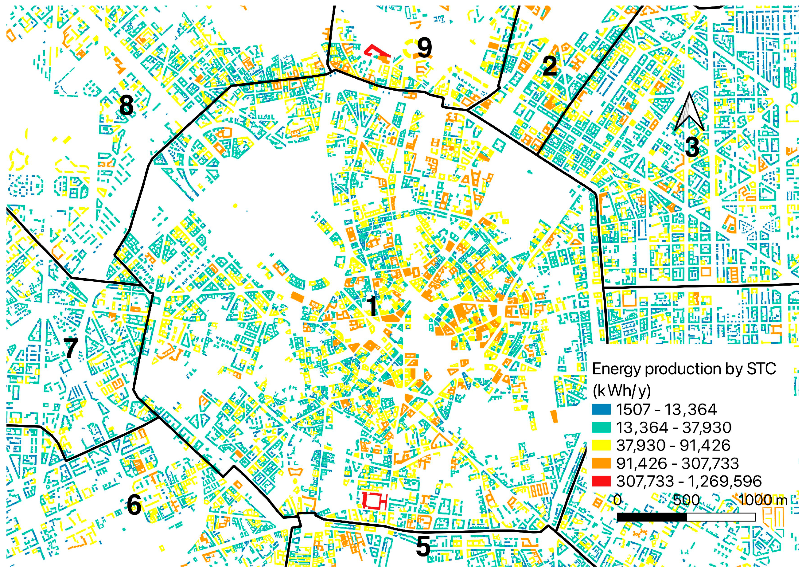
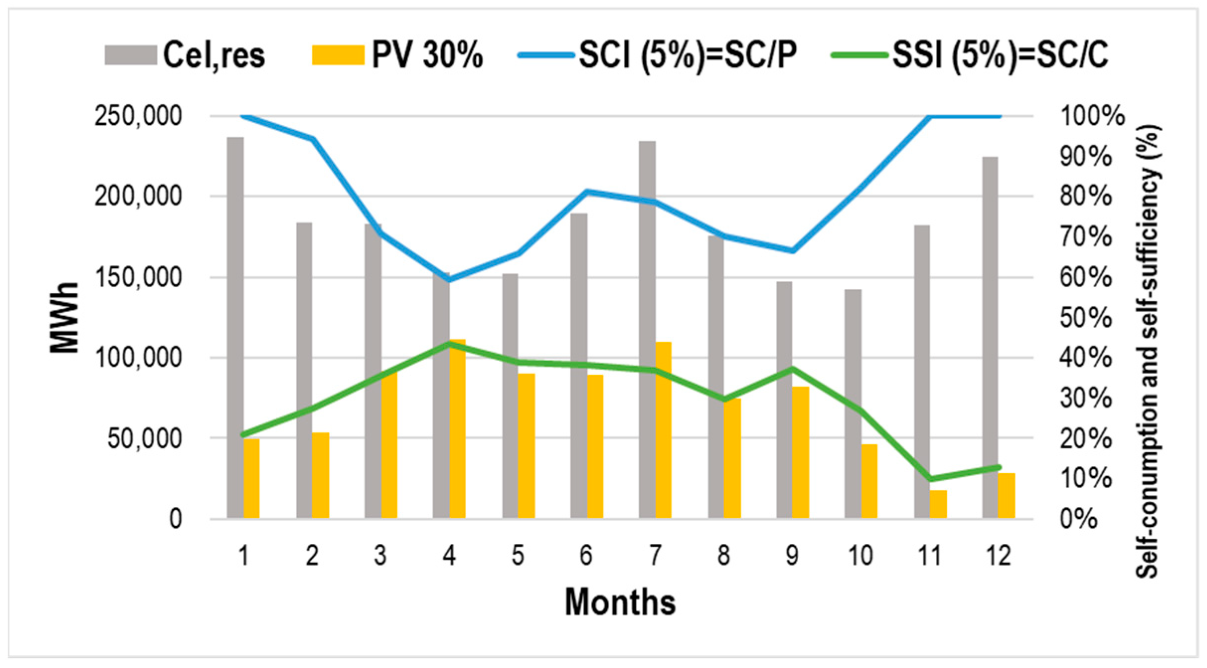
4.4. Evaluation of Solar Irradiation and Energy Production with Roof-Integrated Technologies

Solar energy is among the most widely used renewable sources in the clean energy transition of cities. The wide availability of roof areas and the simplicity of installation, the reduced visual impact and the low price determine a widespread use of solar technologies, especially (but not only) in Italy and southern Europe (but not only). Except in historically and environmentally constrained areas, the visibility of solar technology is indeed positive, indicating the city’s commitment to clean energy and technological progress. The use of solar technology is a first step in promoting responsible consumption and clean production of energy in cities. Consumption can be calculated through the instantaneous quantity of energy produced that meets the energy-use in order to require a lower quantity of fossil fuels [23]. This evaluation can consider the single user, with self-consumption, a condominium with multiple users or a district and, furthermore, a community, with collective self-consumption.

In this section, the evaluation of solar resources and the potential of clean energy production is presented to evaluate energy self-consumption for residential users in each month using roof-integrated solar technologies. For solar analysis, no historical constraints were considered.

Figure 17 explains in detail the QGIS place-based assessment with the building as territorial unit. As already mentioned, a raster image of the DTM with 10 m precision and the area and height of the buildings was used to describe the 3D urban environment (Figure 17, points 1 to 6). The DSM serves to show the evaluation of slope and aspect of each surface of the urban environment, a crucial step for solar analyses.

For the evaluation of solar irradiation, the characteristics of sun and sky should also be defined. They can be explained mainly by two monthly variables: diffuse-to-global irradiation (D/G) and Linke Turbidity Factor (TL) or transmissivity (Figure 17, point 9). Table 8 shows the monthly values for both variables for Milan in wintertime, with higher values of D/G and lower Linke Turbidity Factors, and vice versa in summertime. These data were respectively taken from the website of PVGIS (Last update: 01/03/2022) and Meteonorm 8.1.4 software. A constant albedo of 0.20 was used according to the average value for urban environments.

Then, the daily solar irradiation was calculated with the tool “r.sun.insoltime” for all points every 10 m in the city, especially on the roofs of the buildings. The results of these analyses are raster images, which were processed to have numerical values for solar irradiation.

Solar irradiation could also be an important variable for energy modeling [24] but in this statistical analysis this variable was explained locally by the building density as a surrogate variable. In this work, solar irradiation was used to evaluate solar energy production using either photovoltaic panels (PV) or solar thermal collectors (STC). In this way, in the city of Milan, solar energy can be used to supply DHW, space heating H, and electrical appliances E, reducing consumption especially during the summer season when there is a diurnal and seasonal positive correlation (cooling period). The aim of this analysis was to optimize self-consumption and self-sufficiency, considering for each building the solar exposition, the available area of the roof and the demand profile of the residential users.

Two solar technologies were used to produce energy:

Flat solar thermal collector STC with optical efficiency of 77.5% and heat loss coefficients k₁ = 4.35 and k₂ = 0.01.
Photovoltaic PV panel in monocrystalline silicon with an efficiency of 23%.

In this work, the thermal energy consumption for domestic hot water, evaluated in the previous section, was compared with the solar energy produced by thermal collectors TC; likewise, the electricity consumption was compared with solar energy produced by photovoltaic panel PV. All technologies are roof-integrated.

Figure 18 shows the general methodology for assessing the energy produced by roof-integrated solar technologies. Generally, the quantity of energy produced depends on both area and solar exposition of the panels, but the user demand should be considered too: the energy production should meet the actual and future energy demand. The optimal orientation can be defined by choosing the surface that receives the highest solar irradiation excluding obstacles, but this is not an efficient method for increasing the self-consumption level, because the demand profile changes according to the type of user. For example, for residential users, the peak of electricity demand occurs in the afternoon, which makes it more efficient to analyze different orientations that can fulfill the highest possible self-consumption rather than selecting only the orientation with the highest solar irradiation. Thus, solar production hourly analysis should follow a multi-approach considering the end-user demand profile together with the solar irradiation [24,25].

Similarly to the previous section, the level of accuracy of the input data is very important but some initial evaluations can be made on typical days of the year: winter, summer and mid-season.

The solar irradiance on top of each residential building was calculated for each month in kWh/m². Regarding thermal energy production, a standard flat solar collector has been considered with an average efficiency that changes between 12% in November and 67% in July. In Figure 19, the energy consumption for domestic hot water is represented and it was evaluated knowing the number of inhabitants in each residential building assuming a consumption of 50 L/day/inh and hot water at 45 °C. The blue area in the center of district 1 is the area with offices and commercial buildings without residential users and the DHW load.

Figure 20 represents the use of roof-integrated flat collectors on 5% of the available building roof area. In Milan, the high presence of big condominiums limits the roof area per inhabitant and thus the possibility to meet the energy demand for hot water, especially in wintertime. This sizing of the solar panel area (i.e., 5%) was chosen to avoid extra production of thermal energy in summertime which could be wasted.

Figure 21 illustrates the total amount of electricity generated by photovoltaic panels using 30% of the available roof area, respectively. In this case, this sizing of the photovoltaic area was chosen on the basis of a purely economic–environmental evaluation because the extra production can be sold to the national electrical grid or exchanged between users. As already mentioned, solar irradiation has a positive diurnal and seasonal correlation with space cooling that requires electricity, therefore its over-production in summertime could be used also for space cooling (not included in this analysis).

Table 9 shows the annual energy consumption for space heating, domestic hot water, electricity and the energy production with solar technologies by district. It is possible to observe that the annual energy production by STC is about 73% of the energy consumption; only in the central district 1, with a lower presence of inhabitants, is production about 1.8 times higher than consumption. In this case, the hot water can be used by non-residential users. The energy-use for electricity was calculated based on the population and families of each district, using the hourly profile of electricity consumption per family for the city of Milan: 1500–1800 kWh/inh/year [20,21]. Using the thermal energy consumption in 2017 of 12,200 GWh [23], the mean absolute percentage error (MAPE) with energy consumption for space heating and domestic hot water is 5.2%, which is in the average error range reported in the literature considering urban scale analysis (between 5 and 20%) [26]. It should be also noted that the measured data are related to the specific year of 2017 with its climate condition, while the simulated data using the EPCs’ database consider average 20-year climate conditions.

For environmental and cost–benefit analyses the evaluation of the self-sufficiency SS and self-consumption SC is mandatory. The self-consumer is defined by the European Directive 2018/2001/EU as a user that generates renewable energy for its own consumption without any commercial activity. The ratio between the self-consumption and the total consumption is the self-sufficiency index (SSI) and the ratio between the self-consumption and the total production is the self-consumption index (SCI). The first SSI is important from an environmental and social point of view, whereas the SCI considers the technical and economic investments and benefits. Optimization could be reached with high SSI and high SCI but with solar technologies due to the intrinsic nature of the sun (both daily and seasonal behavior); the SSI is annually lower than 50%.

The sizing of solar technologies is represented in Figure 22. For the supply/demand optimization, it was necessary to divide the simulations for the big city of Milan by districts, to be able to carry out the analyses with a standard personal computer. Figure 22 compares the monthly data of district 2 for energy produced by roof-integrated STC and PV and the consumption for DHW and electricity. In fact, the use of STC has a negative seasonal correlation with space heating loads, so it is more appropriate to use it for domestic hot water production that is quite constant during the year. The monthly consumptions for DHW vary mainly by the number of days in each month and for electricity by the use of space heating (auxiliary elements), space cooling and lighting systems. The variation in solar irradiation and efficiency of STC determines a higher self-sufficiency during summer and a lower one during winter (especially in November). Therefore, for DHW, the annual self-sufficiency index SSI, using 5% of roof area, is 67%, ranging from 8 to 100% during the various months.

The same analysis has been carried out with roof-integrated photovoltaic PV modules using 30% of available roofs (in Figure 22). The relative monthly production of electricity is reported and compared with electrical consumption. The annual self-sufficiency index for PV panels is equal to 30%, ranging monthly from 11 to 48% in the different months.

It is important to analyze the self-consumption level before implementing the STC or PV power systems by assessing the relation between consumption and production to satisfy both higher self-consumption and self-sufficiency levels. It is very important to select a good technology with high efficiency considering climate conditions: air temperature and solar irradiation. This analysis considers instantaneously (e.g., hourly) consumption and production for a specific user.

Utilizing solar technologies can reduce the dependence of residential buildings on conventional systems that commonly rely on fossil fuels. Solar technologies can improve self-sufficiency, supplying energy even during power outages or natural disasters, thus enhancing the buildings’ resilience and sustainability.

Figure 23 analyses the self-sufficiency SSI and self-consumption SCI indexes for STC occupying the 5% of the roof area of residential buildings; it shows that this area is sufficient to completely cover the needs of DHW for the inhabitants from April to September. Integrating renewable energy sources not only reduces carbon emissions but also empowers communities to rely less on energy dependence from abroad, thus reducing countries’ vulnerability to energy price fluctuations and geopolitical uncertainties. It fosters a distributed energy production system that can better withstand unforeseen challenges, making it a crucial step towards a greener and more resilient future.

The monthly PV production and consumption are represented in Figure 24. Consumption is fully covered by production from May till July and almost for August, thanks to high solar irradiation during these months, leading to a high SSI. However, from November till February, the demand is barely covered, with less than 50% of the energy consumption met by PV production alone, resulting in a lower SSI.

Regarding PV generation, the size of the systems depends on cost–benefit analysis, considering also the incentives for PV production and installation costs. In this case, over-production can be economically advantageous but, in this work, the main focus is on achieving self-sufficiency at building or community scale.

To ensure a sustainable and efficient energy supply, it is crucial to implement storage systems to optimize the use of solar technologies throughout the days, aligning it with the demand profile while also increasing the self-consumption index. While satisfying demand, it is equally important not to have over-production, as excessive generation would lead to a decreased self-consumption index. The exchange of energy production between users can lead to more use of the over-production with a higher collective self-consumption and higher self-sufficiency, which is the case for energy communities. Also, by integrating energy storage, excess energy produced during peak hours can be efficiently stored and utilized during hours of lower solar irradiation. The increased focus on self-consumption or collective self-consumption allows for a higher proportion of the locally generated solar energy to be consumed on-site, reducing dependency on external energy sources.

The presented place-based approach considers building energy modeling within an urban context accounting for the effects of the characteristics of each building and urban parameter. This modeling has high potential for estimating energy consumption, production, and related emissions in urban areas, and it can be easily integrated into a platform.

Figure 25 illustrates an example of a platform with integrated urban energy modeling for analyzing the impacts of changing energy-related variables. By controlling buildings and urban attributes (as shown in the middle graph of Figure 25), it becomes possible to obtain valuable insights (right graph), enabling urban planners, architects, and policymakers to make informed decisions when designing future sustainable cities and new energy policies. Starting from a scenario, Figure 25 in black, the results of a future scenario, in grey, can be compared.

With this powerful platform, city planners can foresee and assess the spatial distribution of energy demands, production capacity, and related emissions of various urban development scenarios. Furthermore, the ability to consider diverse urban parameters allows the model to account for the dynamic nature of cities and their evolving energy needs over time. As a result, this approach not only facilitates accurate estimations but also supports the development of resilient cities that are well prepared to meet energy challenges and mitigate environmental impacts.

5. Conclusions

Building energy modeling is becoming an essential tool for analyzing the energy consumption at city scale to achieve more sustainable urban environments. The place-based methodology presented in this work allows the application of UBEMs in various urban contexts and climate conditions. It provides in detail the modeling steps, starting from input data acquisition using open-source databases (Table 2), followed by data pre-processing and modeling using the open-source software QGIS (Figure 15). This statistical modeling completely relies on free geo-databases, and it is important to highlight this step; more available and accurate urban data results in improving the precision of UBEM.

The analysis focused on the residential sector in the city of Milan and on its main forms of energy consumption, which are space heating, domestic hot water, and electricity. The GIS-based approach gives an important insight into the benefits of analyzing and retrofitting the existing building stock for achieving energy efficient cities. The EPC database (from 2016 to 2022) was used to analyze the energy performance of buildings before and after retrofit measures, and to measure their effect on enhancing territories considering all technical, economical, and environmental constraints. The results illustrated in Figure 10 show that 25% of the buildings achieved energy class A, B, or C after the retrofit interventions, while only 7% of them were in these classes before retrofit interventions.

This work describes in detail all the steps for calculating energy-related variables, consumption and production from solar source using QGIS (Figure 17). The produced amount of energy from solar technologies (STC and PV) was analyzed, considering the real 3D urban environment, to evaluate the potential share of energy consumption in the city of Milan. With a standard PV system, the annual SSI can reach 29.1% and 32.1% and the SCI 75.8% and 62.8%, considering the use of 30% and 40% of roof area, respectively. These results show the importance of sizing solar systems properly from an environmental and economic point of view, using both indexes simultaneously, because increasing the solar system area results in higher SSI but lower SCI due to over-production. The solar production analysis highlights the importance of the place-based approach in evaluating the availability of roof areas in urban contexts for energy generation, self-consumption and collective self-consumption with other nearby users.

The statistical energy consumption model was calibrated by comparing the data obtained by the statistical modeling with the energy consumption data reported in the EPC database for the city of Milan. The accuracy of the model is acceptable considering a MAPE of 5.2%, and the error average in the literature, which is 5–20% [26].

The resulting maps help in understanding the energy-related variables clearly, due to the possibility of GIS-based modeling in overlapping the maps for further analysis. For example, the consumption of DHW illustrated in Figure 19 is correlated with the number of families (Figure 4) and the consumption for space heating with the gross volume of residential buildings (Figure 5). For further applications, the presented methodology can be useful to analyze more correlations with newly available input data, e.g., income data.

With the increase in data accessibility, the USEM is believed to achieve higher accuracy levels since the most challenging step is data collection and pre-processing.

Finally, the methodology of this work can help in achieving climate neutral cities by optimizing the spatial distribution of energy demand and supply, boosting energy policy as the increase of retrofit interventions and more use of available renewable energy sources, like the solar source. A further application is the evaluation of the impact of local actions at an urban scale.

Author Contributions

Conceptualization, G.M.; Methodology, G.M. and Y.U.; Software, M.A. and Y.U.; Validation, G.M., M.A. and Y.U.; Data curation, M.A. and F.F.; Writing—original draft, G.M., M.A., A.M. and Y.U.; Writing—review & editing, G.M. and Y.U.; Supervision, G.M. All authors have read and agreed to the published version of the manuscript.

Funding

This research received no external funding.

Institutional Review Board Statement

Not applicable.

Informed Consent Statement

Not applicable.

Data Availability Statement

The results data of this study are not publicly available due to privacy and agreements between research centers.

Acknowledgments

The authors are grateful to the collaboration with Eugenio Morello and Nicola Colaninno, Laboratorio di Simulazione Urbana Fausto Curti, Dipartimento di Architettura e Studi Urbani, Politecnico di Milano, for sharing documents, data and geo-databases for the City of Milano.

Conflicts of Interest

The authors declare no conflict of interest.

Appendix A

The used query to calculate the common surfaces between adjacent buildings:

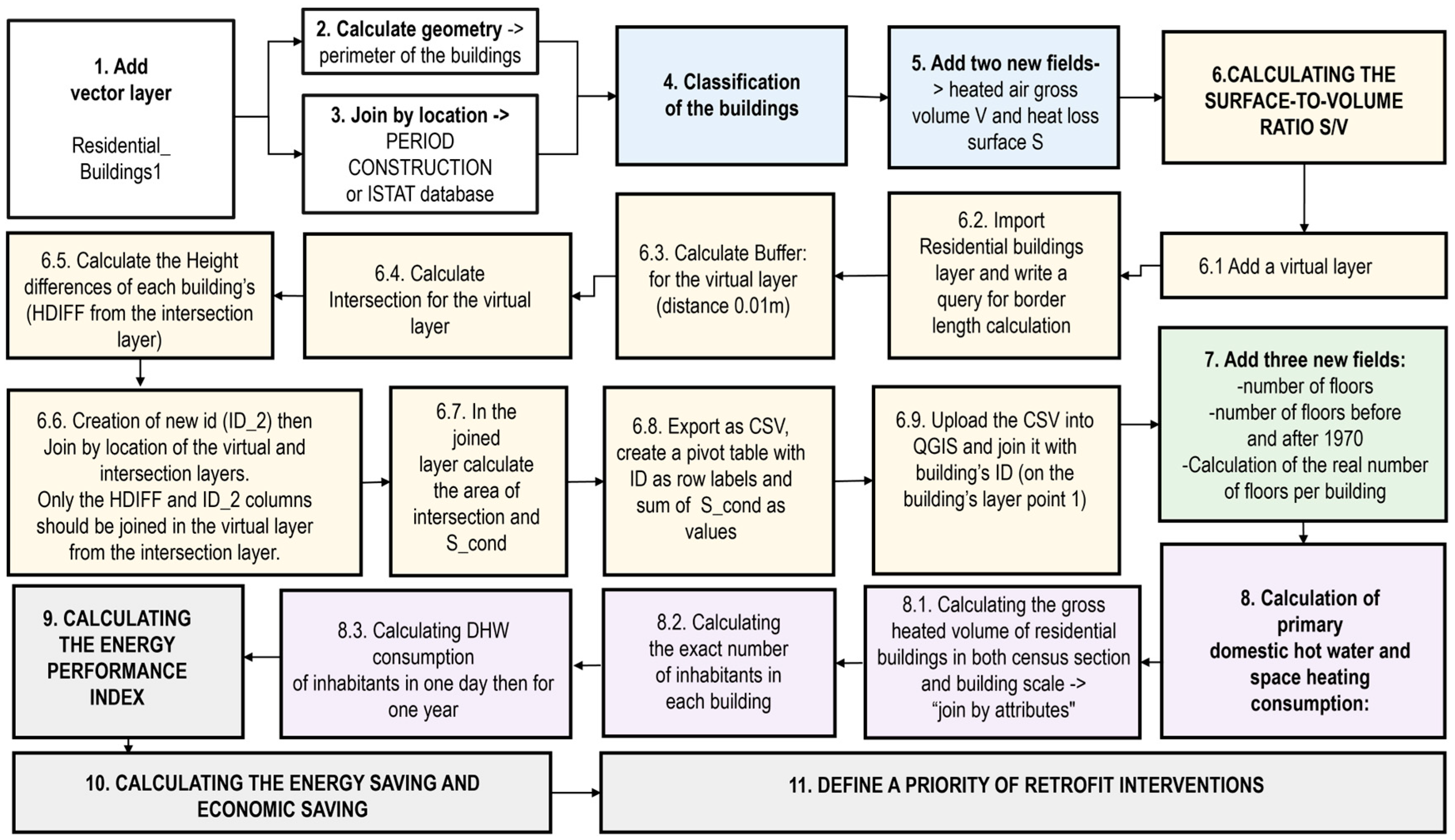
SELECT
a.*,
b.id || ‘, len:’ || round(st_length(st_intersection(a.geom, b.geom)), 4) AS “neighbor_info”
FROM
“building layer” AS a, “building layer” AS b
WHERE
st_intersects(a.geom, b.geom)
AND a.id <> b.id
ORDER BY
a.id ASC

where;

o: round(st_length(st_intersection(a.geom, b.geom)), 4): calculates the length of the intersection between the two geometries (a and b), with a decimal number.
o: AS “neighbor_info”: renames the result of the series as “neighbor_info” and assigns it to a new column in the result set.
o: “building layer”: this should be replaced with the actual name of the building layer. It is the table for using the query, and we use the aliases a and b to reference it twice for the self-join operation.
o: AS a, AS b: These are table aliases. AS is used to give a table a temporary name (a and b in this case) so that it can be used as a reference to the same table multiple times in the query.
o: st_intersects(a.geom, b.geom): checks if the geometries of a and b intersect.
o: a.id <> b.id: ensures that the same polygon is not compared with itself by checking that the id of a is not equal to the id of b. This prevents self-comparisons.
o: a.id ASC: Sorts the result set by the id column of table a in ascending order.

References

Jasiūnas, J.; Lund, P.D.; Mikkola, J. Energy system resilience—A review. Renew. Sustain. Energy Rev. 2021, 150, 111476. [Google Scholar] [CrossRef]
United Nations: Department of Economic and Social Affairs. UN-Energy Plan of Action, May 2022. Available online: https://un-energy.org/wp-content/uploads/2022/05/UN-Energy-Plan-of-Action-towards-2025-2May2022.pdf (accessed on 7 August 2022).
Hasselqvist, H.; Renström, S.; Strömberg, H.; Håkansson, M. Household energy resilience: Shifting perspectives to reveal opportunities for renewable energy futures in affluent contexts. Energy Res. Soc. Sci. 2022, 88, 102498. [Google Scholar] [CrossRef]
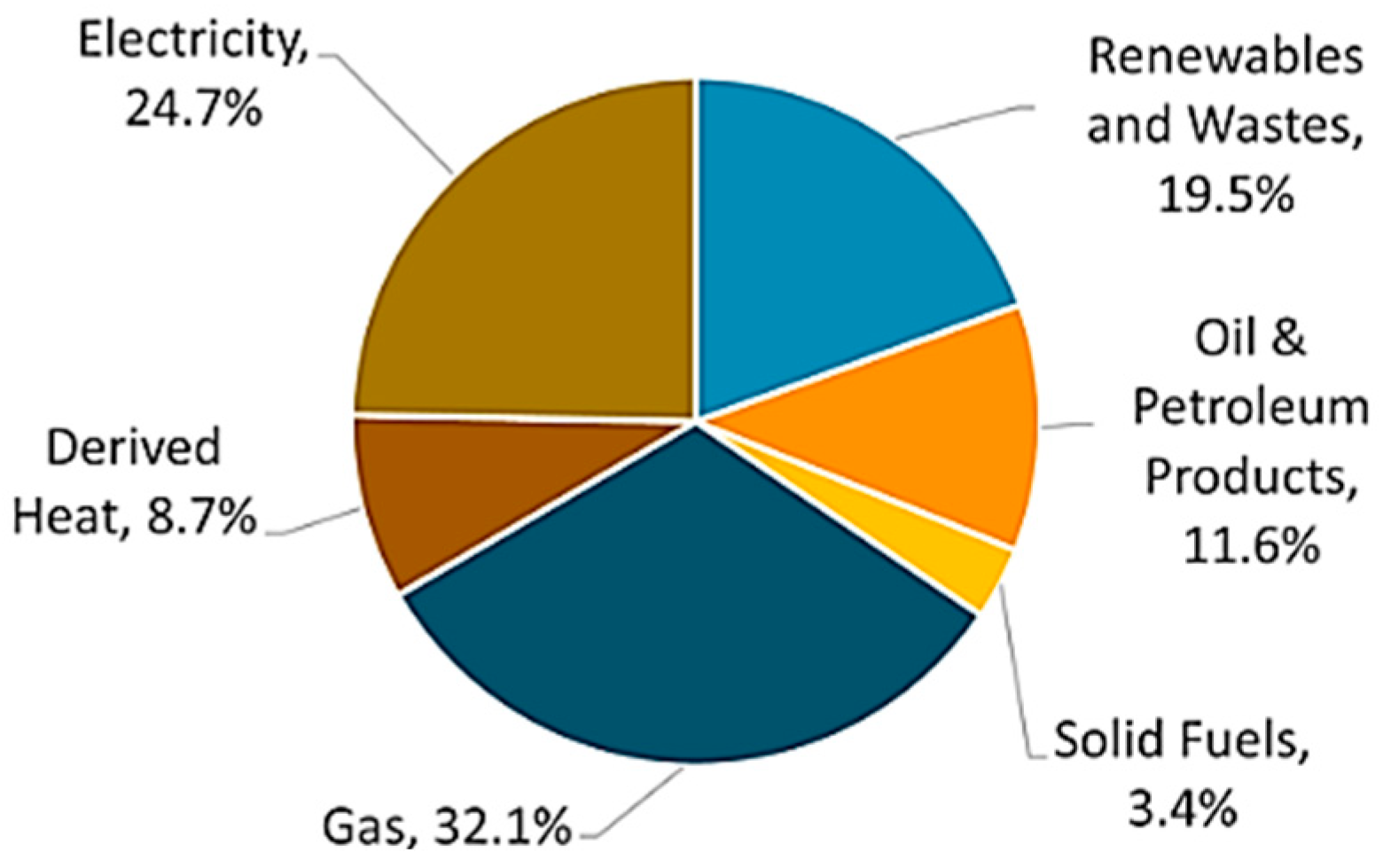
Eurostat: Final Energy Consumption by Sector, EU-27, 2018 (% of Total, Based on Tonnes of Oil Equivalent). Available online: https://ec.europa.eu/eurostat/ (accessed on 20 July 2023).
McKeen, P.; Fung, A. The effect of building aspect ratio on energy efficiency: A case study for multi-unit residential buildings in Canada. Buildings 2014, 4, 336–354. [Google Scholar] [CrossRef]
Duran, A.; Iseri, O.K.; Meral Akgul, C.; Kalkan, S.; Gursel Dino, I. Compiling Open Datasets to Improve Urban Building Energy Models with Occupancy and Layout Data. In Proceedings of the 27th CAADRIA Conference, Sydney, Australia, 9–15 April 2022. [Google Scholar] [CrossRef]
Malhotra, A.; Bischof, J.; Nichersu, A.; Häfele, K.H.; Exenberger, J.; Sood, D.; Allan, J.; Frisch, J.; van Treeck, C.; O’Donnell, J.; et al. Information modelling for urban building energy simulation—A taxonomic review. Build. Environ. 2022, 208, 108552. [Google Scholar] [CrossRef]
Sun, Y.; Haghighat, F.; Fung, B.C. A review of the-state-of-the-art in data-driven approaches for building energy prediction. Energy Build. 2020, 221, 110022. [Google Scholar] [CrossRef]
Database CENED+2—Energy Certification of Buildings in the Municipality of Milan. Available online: https://dati.comune.milano.it/dataset/ds623_database_cened2__certificazione_energetica_degli_edifici_nel (accessed on 20 July 2023).
ISTAT. Quattordicesimo Censimento Generale della Popolazione e delle Abitazioni. 2001. Available online: http://dawinci.istat.it (accessed on 7 August 2023).
UNI 10349:2016; Heating and Cooling of Buildings—Climatic Data. Italian Standardization Entity UNI: Rome, Italy, 2016.
Covenant of Mayors, Sustainable Energy Action Plan 2018. Available online: https://www.covenantofmayors.eu/about/covenant-community/signatories/action-plan.html?scity_id=11832 (accessed on 10 June 2023).
ARPA Lombardia, Atmospheric Emissions Inventory INEMAR (INventario EMissioni ARia). Available online: https://www.inemar.eu/xwiki/bin/view/InemarDatiWeb/Risultati+Regionali (accessed on 10 June 2023). (In Italian).
City of Milan, Air and Climate Plan. Available online: https://www.comune.milano.it/piano-aria-clima (accessed on 10 June 2023). (In Italian).
A New Air and Climate Plan for Milan. Available online: https://eit.europa.eu/news-events/news/new-air-and-climate-plan-milan (accessed on 10 June 2022).
Padovani, C.; Salvaggio, C. Strategia per la sostenibilità ambientale e resilienza urbana nel Pgt della Città di Milano: Il Piano aria clima. In Pianificazione Urbana e Territoriale dalla Lezione di Giampiero Vigliano alle Prospettive del Green New Deal—Urbanistica Dossier; Istituto Nazionale di Urbanistica: Rome, Italy, 2022; Volume 27, pp. 117–119. ISBN 9788876032417. Available online: http://www.inuedizioni.com/it/prodotti/rivista/n-027-urbanistica-dossier (accessed on 20 July 2023). (In Italian)
EU Project: Cities on Power. Available online: https://keep.eu/programmes/119/2007-2013-Central-Europe/ (accessed on 20 July 2023).
Mutani, G.; Todeschi, V. GIS-based urban energy modelling and energy efficiency scenarios using the energy performance certificate database. Energy Effic. 2020, 14, 47. [Google Scholar] [CrossRef]
Mutani, G.; Todeschi, V.; Beltramino, S. Energy consumption models at urban scale to measure energy resilience, Sustainability—Bridging the Gap: The Measure of Urban Resilience. Sustainability 2020, 12, 5678. [Google Scholar] [CrossRef]
Energia Lombardia. Available online: https://www.energialombardia.eu/energia-e-territorio#:~:text=Per%20quanto%20attiene%20i%20consumi,0%2C1%20tep%20procapite (accessed on 10 June 2023). (In Italian).
ARERA (Regulatory Authority for Energy, Networks and Environment), Analysis of Consumption of Domestic Customers. Available online: https://www.arera.it/it/dati/mr/mr_consumiele.htm (accessed on 10 June 2023). (In Italian).
Ghoshchi, A.; Zahedi, R.; Pour, Z.; Ahmadi, A. Machine Learning Theory in Building Energy Modeling and Optimization: A Bibliometric Analysis. J. Mod. Green Energy 2022, 1, 4. [Google Scholar] [CrossRef]
“PIANO ARIA E CLIMA” del Comune di Milano. Available online: https://www.comune.milano.it/documents/20126/430903598/sub+Allegato+4+-+Mitigazione.pdf/b672b7bd-201e-dc47-fb03-e7453faae745?t=1652093322345 (accessed on 10 June 2023). (In Italian).
Mutani, G.; Todeschi, V. Optimization of Costs and Self-Sufficiency for Roof Integrated Photovoltaic Technologies on Residential Buildings. Energies 2021, 14, 4018. [Google Scholar] [CrossRef]
Huld, T.; Müller, R.; Gambardella, A. A new solar radiation database for estimating PV performance in Europe and Africa. Sol. Energy 2012, 86, 1803–1815. [Google Scholar] [CrossRef]
Davila, C.C.; Reinhart, C.F.; Bemis, J.L. Modeling Boston: A workflow for the efficient generation and maintenance of urban building energy models from existing geospatial datasets. Energy 2016, 117 Pt 1, 237–250. [Google Scholar] [CrossRef]

Figure 1. Final energy consumption of residential sector by source (EU-27, 2018) [4].

Figure 2. Description of statistical energy modeling with a place-based methodology.

Figure 3. Periods of construction for the buildings in district 2.

Figure 4. Number of families per building in district 2.

Figure 5. Residential buildings’ gross volume in district 9.

Figure 6. Building typologies for the 9 districts of the city of Milan.

Figure 7. DSM for the central district in Milan (with points every 10 m).

Figure 8. EPC analysis for energy modeling flowchart.

Figure 9. Typical tasks in the energy domain and their corresponding paradigm in the Machine Learning.

Figure 10. Energy classes of buildings before (a) and after (b) retrofit interventions by districts (1–9).

Figure 11. EPCs analysis: retrofitted heated surfaces per year (a), energy savings per year after retrofit (b). (Red points indicate the non-complete years 2015 and 2022).

Figure 12. Buildings’ density (m³/m²) in census sections in the city of Milan.

Figure 13. (a) Energy performance EP_gl,nren of residential buildings in Milan before retrofit interventions. (b) Energy performance EP_gl,ren of residential buildings in Milan after retrofit interventions.

Figure 14. Energy performance EP_gl,nren of buildings based on building density categories by period of construction in Milan before retrofit interventions.

Figure 15. Description of the tools used in QGIS for place-based methodology.

Figure 16. District 1: annual space heating specific consumption (kWh/m²/y) for residential buildings in district 2.

Figure 17. Description of DSM realization and solar irradiation calculation.

Figure 18. Methodology for assessing energy production with roof-integrated solar production.

Figure 19. Annual DHW consumption for the central district 1.

Figure 20. Annual energy production with roof-integrated Solar Thermal Collectors in district 1.

Figure 21. Annual energy production with roof-integrated photovoltaic panels in district 1.

Figure 22. Monthly energy consumption and production with solar thermal collectors for district 2 (STC, 5% roof area) and photovoltaic modules (PV, 30% of roof area).

Figure 23. Monthly energy consumption for DHW and production by STC with 5% of roof area.

Figure 24. Monthly energy consumption for electricity and PV production with 30% of roof area.

Figure 25. Urban energy modeling platform: actual and future energy scenario.

Table 1. Average monthly air temperature and solar irradiation in Milan [11].

	1	2	3	4	5	6	7	8	9	10	11	12
T_avg °C	4.0	7.1	10.6	13.4	19.4	22.8	24.5	24.3	19.8	14.1	7.5	3.5
I, kWh/m²	42.2	53.4	101.6	133.3	163.6	190.8	200.6	164.5	126.7	68.9	35.8	31.0

Table 2. Sources for data collection and pre-processing phases for place-based modeling of energy consumption and actual/future production in Italy.

Typology	Input Data	Typology	Source	License
Energy consumption models and energy-related variables
Built-up environment/Urban morphology/Type of users	Regional-Municipal data by Participatory Mapping”	OpenStreetMap	https://download.geofabrik.de/ (accessed on 20 July 2023) https://download.geofabrik.de/europe/italy.html (accessed on 20 July 2023) https://osmit-estratti.wmcloud.org/ (accessed on 20 July 2023) (for Region and Municipality)	Open Data Commons Open Database License (ODbL)
	Public Buildings	Treasure Dept	Dati immobili al 31/12/2018—MEF Dipartimento del Tesoro	CC-BY 4.0
	Territorial Geo-topographic Database (BDTRE)	Italian Regions	Piedmont Region: https://www.geoportale.piemonte.it/cms/bdtre/modalita-di-pubblicazione-e-fruizione (accessed on 20 July 2023); City of Turin: http://geoportale.comune.torino.it/web/cartografia/cartografia-scarico (accessed on 20 July 2023); Lombardy Region: https://www.geoportale.regione.lombardia.it/download-ricerca (accessed on 20 July 2023); City of Milan: https://geoportale.comune.milano.it/sit/open-data/ (accessed on 20 July 2023)	CC-BY 4.0 International
	Digital Terrain/Elevation/Surface Model (DTM, DEM, DSM) for Italy	SINAnet—DEM (20 m)	ISPRA: http://www.sinanet.isprambiente.it/it/sia-ispra/download-mais/dem20/view (accessed on 20 July 2023)	IODL License https://www.dati.gov.it/content/italian-open-data-license-v20 (accessed on 20 July 2023)
		TINITALY—DTM (10 m)	Istituto Nazionale di Geofisica e Vulcanologia (INGV, National Institute of Geophysics and Volcanology): https://data.ingv.it/dataset/185#additional-metadata (accessed on 20 July 2023)	CC BY
		DTM 20 m	IGM- Military Geographical Institute: http://www.pcn.minambiente.it/mattm/catalogo-metadati/ (accessed on 20 July 2023); http://www.pcn.minambiente.it/mattm/visualizzazione-metadati/?keyword=digital+terrain+model&rid=local (accessed on 20 July 2023) Free GIS data for Italy: https://freegisdata.org/place/106881/ (accessed on 20 July 2023) (information only)	Creative Commons Attribution 4.0 International
		DTM 20–40–75 m	ISPRA Higher Institute for Environmental Protection and Research: http://dati.isprambiente.it/ (accessed on 20 July 2023)	Licence
		DSM 1 m (Italy)	Ministry of Ecological Transition (MITE): http://www.pcn.minambiente.it/mattm/visualizzazione-metadati/?keyword=dsm&rid=local (accessed on 20 July 2023)	and open data
	Satellite images (Landsat 8)	Raster 30 m × 30 m	https://earthexplorer.usgs.gov/ (accessed on 20 July 2023) https://www.usgs.gov/coastal-changes-and-impacts/gmted2010 (accessed on 20 July 2023)	No restrictions, all GMTED2010 data products are available
	Orthophotos	Color orthophoto AGEA 2009–2012	Ministry of Ecological Transition (MITE): http://www.pcn.minambiente.it/mattm/visualizzazione-metadati/?keyword=ortofoto&rid=local&paged_e=1 (accessed on 20 July 2023)	Open data
		Color and b&w digital Orthophoto	Free GIS data for Italy: https://freegisdata.org/place/106881/ (accessed on 20 July 2023) (information only)	Open data
	Land use/cover	SINAnet—CORINE Land Cover (Italy)	1990: https://groupware.sinanet.isprambiente.it/uso-copertura-e-consumo-di-suolo/library/copertura-del-suolo/corine-land-cover/corine-land-cover-1990 (accessed on 20 July 2023) 2000: https://groupware.sinanet.isprambiente.it/uso-copertura-e-consumo-di-suolo/library/copertura-del-suolo/corine-land-cover/corine-land-cover-2000 (accessed on 20 July 2023) 2018: https://groupware.sinanet.isprambiente.it/uso-copertura-e-consumo-di-suolo/library/copertura-del-suolo/corine-land-cover/clc2018_shapefile (accessed on 20 July 2023)	IODL License
	Land use/cover	SINAnet—Land taking	https://groupware.sinanet.isprambiente.it/uso-copertura-e-consumo-di-suolo/library/consumo-di-suolo (accessed on 20 July 2023)	CC BY SA 3.0 IT
	European statistics about Environment & Energy and SDGs	EUROSTAT	https://ec.europa.eu/eurostat/data/database (accessed on 20 July 2023)	Open Data
Socio-economic characteristics	Population, housing, industry and services census section data Industry and services	National Institute of Statistics ISTAT—Territory and census data	ISTAT: https://www.istat.it/it/archivio/104317 (accessed on 20 July 2023) “Basi Territoriali e Variabili Censuarie” (new data will be available at: https://www.istat.it/it/archivio/6789 (accessed on 20 July 2023)) Census of population and housing and of industry and services (txt-xls-csv) 2011 http://dati.istat.it/Index.aspx?DataSetCode=DCIS_POPRES1 (accessed on 20 July 2023)	Open Data
Climate data	Air temperature, relative humidity, wind velocity, solar irradiation, heating degree days (HDD)	Climate data	JRC: https://re.jrc.ec.europa.eu/pvg_tools/en/tools.html (accessed on 20 July 2023) Italian Standard UNI 10349-1, -2, -3:2016 (Italian Standardization Body)	PVGIS © European Communities, 2001–2021
Climate data		Climate data	EnergyPlus: https://energyplus.net/weather (accessed on 20 July 2023)	Open data: https://energyplus.net/weather/sources (accessed on 20 July 2023)
Energy consumption data	Sustainable Energy and Climate Action Plan (SEAP-SECAP)	Covenant of Mayors—Europe	https://eu-mayors.ec.europa.eu/en/home (accessed on 20 July 2023) https://www.covenantofmayors.eu/plans-and-actions/action-plans.html (accessed on 20 July 2023)	Website coordinated by the Covenant of Mayors Office, European Commission.
	Residential user profile for electricity (Province and Regional; 2021–2022)	ARERA (Regulatory Authority for Energy, Networks and Environment)	https://www.arera.it/it/dati/mr/mr_consumiele.htm (accessed on 20 July 2023)	Open Data
	Measurements	‘e-distribuzione’ portal	https://private.e-distribuzione.it/PortaleClienti/PED_SiteLogin (accessed on 20 July 2023)	Confidential-private information
	Surveys/monitoring of electrical energy	TERNA (Electricity Transmission National Grid) Driving Energy	https://www.terna.it/it/sistema-elettrico/transparency-report/total-load (accessed on 20 July 2023) (per bidding-zone)	Open Data Copyright TERNA
	Energy costs (withdrawing costs of electricity and fuels)	ARERA, Consumer Protection Centre and WTRG Economics	ARERA (Regulatory Authority for Energy Networks and The Environment) https://www.arera.it/it/dati/gp27new.htm (accessed on 20 July 2023) (natural gas) https://www.arera.it/it/dati/eep35.htm (accessed on 20 July 2023) (electricity) and https://www.consumer.bz.it/it/confronto-prezzi-combustibili-riscaldamento-alto-adige (accessed on 20 July 2023) (fuels for space heating) and http://www.wtrg.com/daily/crudeoilprice.html (accessed on 20 July 2023) (crude oil)	Open Data Copyright ARERA Copyright 1999–2022 by James L. Williams
	Thermal plants/systems	Registry for thermal plants/systems—Lombardy Region	https://www.dati.lombardia.it/Energia/Catasto-Unico-Regionale-Impianti-Termici-Impianti-/d7i4-7rpy (accessed on 20 July 2023) https://dati.comune.milano.it/dataset/ds598_catasto_unico_regionale_impianti_termici__impianti_targati_n (accessed on 20 July 2023)	Open Data CC
	Energy Performance Certificates (EPCs) database of buildings	CENED and CENED+2 Lombardy Region Piedmont Region	https://dati.comune.milano.it/dataset/ds604_cened__certificazione_energetica_degli_edifici_nel_comune_di (accessed on 20 July 2023) https://dati.comune.milano.it/dataset/ds623_database_cened2__certificazione_energetica_degli_edifici_nel (accessed on 20 July 2023) https://www.geoportale.piemonte.it/geonetwork/srv/ita/catalog.search#/metadata/r_piemon:42f87394-4ec6-4764-bdf8-57bc12d4e0f2 (accessed on 20 July 2023)	Open Data CC BY
Energy production models
Energy production data	Surveys/monitoring of electrical energy	TERNA (Electricity Transmission National Grid) Driving Energy	https://www.terna.it/it/sistema-elettrico/transparency-report/actual-generation (accessed on 20 July 2023) (per primary energy source)	Open Data Copyright TERNA
	Revenue for electricity production in the national grid (per zone and month, Prezzo Zonale Orario PO)	Energy Services Management GSE	https://www.gse.it/servizi-per-te/fotovoltaico/ritiro-dedicato/regolazione-economica-del-servizio (accessed on 20 July 2023) https://www.gse.it/servizi-per-te/fotovoltaico/ritiro-dedicato/documenti (accessed on 20 July 2023)	Open Data Copyright GSE
	Type of technological system and power installed	‘Atlaimpianti’ (Energy Services Management GSE) online portal	https://www.gse.it/dati-e-scenari/atlaimpianti (accessed on 20 July 2023)	Database pursuant to art. 1 L. 22/4/1941 n. 633, as amended by Leg. Decree 6/5/1999 n. 169
	Global Atlas for Renewable Energy	IRENA	International Renewable Energy Agency IRENA: https://www.irena.org/globalatlas (accessed on 20 July 2023)	Open Data Copyright IRENA
	Thermal plants/systems	Regional Land Registry for thermal plants/systems—Lombardy Region	https://www.dati.lombardia.it/Energia/Catasto-Unico-Regionale-Impianti-Termici-Impianti-/d7i4-7rpy (accessed on 20 July 2023) https://dati.comune.milano.it/dataset/ds598_catasto_unico_regionale_impianti_termici__impianti_targati_n (accessed on 20 July 2023)	Open Data CC 0
	Energy prices by time and zone of the electricity produced and fed into the grid (electricity)	Energy Services Management GSE S.p.A.	https://www.gse.it/servizi-per-te/fotovoltaico/ritiro-dedicato/documenti (accessed on 20 July 2023) under “Parola Chiave” type “Ritiro Dedicato”— under “Tipologia” select “Altri Contenuti”	Open Data CC BY NC SA
Energy potential production models
Built-up environment/Urban morphology	Regional-Municipal data by “Participatory Mapping”	OpenStreetMap	https://download.geofabrik.de/ (accessed on 20 July 2023) https://download.geofabrik.de/europe/italy.html (accessed on 20 July 2023) https://osmit-estratti.wmcloud.org/ (accessed on 20 July 2023) (Region and Municipality)	Open Data Commons Open Database License (ODbL)
	Territorial Geo-topographic Database (BDTRE)	Italian Regions (in Italian)	e.g., Piedmont Region: https://www.geoportale.piemonte.it/cms/bdtre/modalita-di-pubblicazione-e-fruizione (accessed on 20 July 2023)	CC-BY 4.0 International
	Digital Terrain/Surface/Elevation Model (DEM, DSM, DTM) Digital Elevation Model	SINAnet—DEM (20 m) (Italy)	ISPRA: http://www.sinanet.isprambiente.it/it/sia-ispra/download-mais/dem20/view (accessed on 20 July 2023)	IODL License https://www.dati.gov.it/content/italian-open-data-license-v20 (accessed on 20 July 2023)
		DEM 10 m (Italy)	Istituto Nazionale di Geofisica e Vulcanologia (INGV): https://data.ingv.it/dataset/185#additional-metadata (accessed on 20 July 2023)	CC_BY
		DSM 1 m (Italy)	Ministero della Transizione Ecologica: http://www.pcn.minambiente.it/mattm/visualizzazione-metadati/?keyword=dsm&rid=local (accessed on 20 July 2023)	Open data
Renewable energy sources	Solar radiation data	Photovoltaic GIS, JRC	https://re.jrc.ec.europa.eu/pvg_tools/it/tools.html (accessed on 20 July 2023)	PVGIS © European Communities, 2001–2021
		Italian Solar Atlas ENEA	National Agency for New Technologies, Energy and Sustainable Economic Development: http://www.solaritaly.enea.it/ (accessed on 20 July 2023)	CC-BY-SA
		Linke Turbidity Factor Worldwide	SODA: https://www.soda-pro.com/help/general-knowledge/linke-turbidity-factor (accessed on 20 July 2023)	CAMS License Agreement and Privacy Statement with License Agreement for SoDa
		COP—Solar Portal for Torino Metropolitan City	Cities On Power Project: https://keep.eu/projects/5551/Cities-on-Power-EN/ (accessed on 20 July 2023) http://energia.sistemapiemonte.it/ittb-torino (accessed on 20 July 2023)	Open Data
	Biomass data	Italian Biomass Atlas ENEA (2017–2020)	National Agency for New Technologies, Energy and Sustainable Economic Development Biomass Atlas: http://atlantebiomasse.brindisi.enea.it/atlantebiomasse/ (accessed on 20 July 2023)	Copyright 2016 ENEA—Atlante delle Biomasse
	Biomass data	National organization ‘Risi’ (Rices)	http://www.enterisi.it/servizi/Menu/dinamica.aspx?idSezione=17505&idArea=17548&idCat=17552&ID=17552&TipoElemento=categoria (accessed on 20 July 2023)	Legal notes
	Waste to energy (i.e., waste production per capita)	Waste institute (ISPRA)	ISPRA Higher Institute for Environmental Protection and Research: https://www.catasto-rifiuti.isprambiente.it/index.php?pg=&width=1093&height=615 (accessed on 20 July 2023)	CC-BY
	Wind data	Italian Wind Atlas RSE	http://atlanteeolico.rse-web.it/ (accessed on 20 July 2023)	Copyright RSE S.p.A.
		Global Wind Atlas 3.1	https://globalwindatlas.info/en/area/Italy (accessed on 20 July 2023)	DTU Wind Energy
		Meteorological institute ‘CMWF Reading	ECMWF European Centre for Medium-Range Weather Forecasts: https://www.ecmwf.int/en/forecasts (accessed on 20 July 2023)	For researchers licence for non-commercial use
	Sea velocity, temperature, salinity, wave height, mean wave period and wave energy	ENEA	National Agency for New Technologies, Energy and Sustainable Economic Development https://climaweb.casaccia.enea.it/WW3MED/details.php (accessed on 20 July 2023) https://giotto.casaccia.enea.it/forecasts/ (accessed on 20 July 2023)	Property of ENEA (SSPT-MET-CLIM Lab)
	Global Atlas for Renewable Energy	International Renewable Energy Agency IRENA	https://www.irena.org/globalatlas (accessed on 20 July 2023)	Open Data Copyright IRENA
Constraints	Soil protection repository	National Repository of interventions for Soil Protection (ReNDiS)	http://www.datiopen.it/it/catalogo-opendata/file-shp (accessed on 20 July 2023)	The Italian portal of Open Data: property of Sistemi Territoriali S.r.l. © 2012
	Land use and hazards	Landslides, floods, avalanches, seismic, fires, ect	ISPRA Higher Institute for Environmental Protection and Research: http://dati.isprambiente.it/ (accessed on 20 July 2023) Free GIS data for Italy: https://freegisdata.org/place/106881/ (accessed on 20 July 2023) (information only)	Creative Commons Attribution 4.0 International Open data
	Maps showing soil protection	Energy Services Management GSE S.p.A.	https://www.gse.it/documenti_site/Documenti%20GSE/Studi%20e%20scenari/Regolazione%20regionale%20FER%2031_12_2020.pdf (accessed on 20 July 2023)	Gestore dei Servizi Energetici—GSE S.p.A

Table 3. Number of EPCs by period of construction and energy classes.

Energy Classes	Period of Construction
Energy Classes	<1930	1930–1945	1946–1960	1961–1976	1977–1992	1993–2006	>2006
A4	39	40	51	36	50	7	3045
A3	91	57	90	38	23	19	3580
A2	117	160	288	192	95	63	3436
A1	178	160	494	444	170	68	2701
B	227	273	552	698	217	277	1638
C	711	897	1600	2098	541	1035	1479
D	2979	3209	5549	6982	1445	2322	1553
E	5537	6275	10,115	12,756	2279	2181	1092
F	7871	9831	16,510	19,949	2676	1375	752
G	8121	10,507	17,346	19,626	2178	560	418

Table 4. Energy performance certificates (EPCs) of residential buildings by motivation of release.

Motivation of EPC Release
Energy Class and Average EP_gl,nren	New Buildings	Retrofitted Buildings	Sale and Lease of Buildings
A4 28 kWh/m²/y	2414	395	309
A3 48 kWh/m²/y	2673	626	281
A2 68 kWh/m²/y	2274	1003	584
A1 79 kWh/m²/y	1291	1421	1093
B 99 kWh/m²/y	132	1057	2037
C 118 kWh/m²/y	39	1520	5882
D 139 kWh/m²/y	44	2638	18,686
E 158 kWh/m²/y	55	2777	33,268
F 189 kWh/m²/y	84	3294	49,617
G 277 kWh/m²/y	99	2054	52,109

Table 5. Average and median values for energy performance indexes (energy need for space heating EP_H,nd and primary energy EP_gl,nren) for residential buildings in Milan.

Energy Performance EP (kWh/m²/y)	EP_H,nd Total	EP_gl,nren Total	EP_gl,nren Non-Retrofitted	EP_gl,nren Retrofitted
N. of dwellings	189,756	189,756	163,866	25,890
Average EP	98.64	187.86	199.52	114.05
Median EP	83.80	167.70	88.73	90.42

Table 6. Pearson’s correlation for variables with EP indexes.

Pearson’s Correlation	EP_gl,nren	EP_H,nd
Period of construction	−42.3%	−41.6%
S/V ratio (m²/m³)	38.6%	46.9%
CO₂ emissions	78.4%	63.9%
Potential energy performance 1	45.5%	44.8%
Potential energy performance 2	79.1%	72.5%
Year of installation of space heating system 1	−31.6%	−26.5%
Year of installation of domestic hot water system 2	−27.0%	−25.6%
Foreigners’ persons residing in Italy over 54 years old	6.2%	5.9%
Resident illiterate population	4.5%	4.4%
Resident families with 1 member	5.1%	2.5%
Population aged 15 and over housewives	5.5%	2.6%

Table 7. Number of buildings analysed by classes of S/V and period of construction for residential non-retrofitted and retrofitted buildings (in brackets).

Period of Construction	Classes of S/V (m²/m³)					Number of Buildings
Period of Construction	<0.2	0.2–0.5	0.51–0.8	0.81–1.1	>1.1	Number of Buildings
<1930 & 1930–1945	2140 (80)	14,133 (738)	5941 (437)	924 (45)	193 (8)	23,332 (1308)
1946–1960	489 (23)	11,419 (210)	13,462 (141)	2003 (19)	355 (2)	27,727 (395)
1961–1970	1261 (23)	19,588 (283)	6645 (147)	741 (21)	73 (6)	28,309 (480)
1971–1980	686 (11)	11,293 (178)	3884 (91)	428 (11)	43 (3)	16,333 (294)
1981–1990	397 (4)	3648 (200)	1539 (111)	178 (0)	22 (0)	5784 (315)
1991–2000 & 2001–2005	152 (0)	2504 (8)	1271 (10)	188 (0)	12 (1)	4127 (19)
>2006	193 (37)	7430 (692)	4174 (400)	514 (57)	46 (1)	12,357 (1187)

Table 8. Monthly data of diffuse-to-global radiation (D/G) and Linke turbidity factor (TL).

	1	2	3	4	5	6	7	8	9	10	11	12
D/G	0.54	0.51	0.46	0.44	0.43	0.40	0.35	0.38	0.42	0.52	0.59	0.59
TL	2.74	2.98	3.5	3.91	3.85	3.9	3.67	3.54	3.45	3.4	3.02	2.72

Table 9. Annual energy-use for space heating and DHW, and solar energy production for the different districts in Milan.

District No.	Energy-Use for Space Heating (kWh_t)	Energy-Use for Domestic Hot Water (kWh_t)	Energy-Use for Electricity (kWh_e)	Energy Production with PV (kWh_e)	Energy Production with STC (kWh_t)	Main Period of Construction
1	966,262,459	70,622,702	159,492,639	134,778,376	124,714,482	Before 1919
2	1,320,954,361	105,323,577	237,860,272	92,261,859	85,416,638	1919–1945
3	1,297,445,750	103,449,166	233,627,147	94,075,251	87,083,751	1919–1945
4	1,352,919,902	113,009,059	255,216,982.6	87,760,731	81,229,151	1946–1960
5	1,066,383,008	89,074,704	201,164,202.8	69,278,538	64,136,604	1946–1960
6	1,288,344,047	107,615,054	243,035,290	69,681,565	64,524,164	1946–1960
7	1,495,087,787	124,884,306	282,035,761	93,955,781	86,975,366	1946–1960
8	1,594,529,076	133,190,612	300,794,525	101,970,262	94,403,965	1946–1960
9	1,472,543,840	129,151,277	291,672,186	101,399,317	93,906,003	1961–1970

Disclaimer/Publisher’s Note: The statements, opinions and data contained in all publications are solely those of the individual author(s) and contributor(s) and not of MDPI and/or the editor(s). MDPI and/or the editor(s) disclaim responsibility for any injury to people or property resulting from any ideas, methods, instructions or products referred to in the content.

© 2023 by the authors. Licensee MDPI, Basel, Switzerland. This article is an open access article distributed under the terms and conditions of the Creative Commons Attribution (CC BY) license (https://creativecommons.org/licenses/by/4.0/).

Share and Cite

MDPI and ACS Style

Mutani, G.; Alehasin, M.; Usta, Y.; Fiermonte, F.; Mariano, A. Statistical Building Energy Model from Data Collection, Place-Based Assessment to Sustainable Scenarios for the City of Milan. Sustainability 2023, 15, 14921. https://doi.org/10.3390/su152014921

AMA Style

Mutani G, Alehasin M, Usta Y, Fiermonte F, Mariano A. Statistical Building Energy Model from Data Collection, Place-Based Assessment to Sustainable Scenarios for the City of Milan. Sustainability. 2023; 15(20):14921. https://doi.org/10.3390/su152014921

Chicago/Turabian Style

Mutani, Guglielmina, Maryam Alehasin, Yasemin Usta, Francesco Fiermonte, and Angelo Mariano. 2023. "Statistical Building Energy Model from Data Collection, Place-Based Assessment to Sustainable Scenarios for the City of Milan" Sustainability 15, no. 20: 14921. https://doi.org/10.3390/su152014921

Note that from the first issue of 2016, this journal uses article numbers instead of page numbers. See further details here.

Article Menu

Statistical Building Energy Model from Data Collection, Place-Based Assessment to Sustainable Scenarios for the City of Milan

Abstract

1. Introduction

2. The City of Milan

3. Materials and Methods

3.1. Data Collection

3.1.1. Energy Performance Certificates Database

3.2. Pre-Processing and Geographical Database Creation

3.3. Statistical Modeling of Buildings’ Energy Consumption

Description of Alternative Machine Learning Models

4. Results and Discussion

4.1. Energy Performance Certificates (EPC) Analysis

4.2. GIS-Based Energy Modeling and Sensitivity Analysis

4.3. Statistical Energy Consumption Model

4.4. Evaluation of Solar Irradiation and Energy Production with Roof-Integrated Technologies

5. Conclusions

Author Contributions

Funding

Institutional Review Board Statement

Informed Consent Statement

Data Availability Statement

Acknowledgments

Conflicts of Interest

Appendix A

References

Share and Cite

Article Metrics

Article Access Statistics

Further Information

Guidelines

MDPI Initiatives

Follow MDPI