Effects of Photovoltaic Solar Farms on Microclimate and Vegetation Diversity

Abstract

The need for energy and the increasing importance of climate change mitigation are leading to a conversion from conventional to renewable energy sources. Solar photovoltaic (PV) power has seen the most significant increase among all renewable energy sources. However, most of these installations are land-based, significantly changing global land use (LU). The real impacts, whether positive or negative, are poorly understood. This study was undertaken to have a better understanding of the impacts of solar parks on the microclimate and vegetation dynamics. First, different solar parks were visited to take measurements of the surface temperature (T_surf), photosynthetic active radiation (PAR), air temperature (T_air), and humidity (RH) to quantify the microclimate and perform a vegetation relevé. The measurements were taken at different positions: underneath, in between, and outside solar panels. For vegetation, the data were first converted to diversity indices, which in turn contributed to a multi-indicator land use impact assessment that evaluated effects on vegetation, biodiversity, soil and water. Solar parks had clear effects on microclimate: if the panels were high enough from the ground, they could lower the T_surf by providing shade and enough airflow. Additionally, the multidimensional functional diversity (FD) analysis of the vegetation indicated that there was less light at a higher humidity and lower temperature underneath the panels. Interestingly, the species underneath the panels also preferred a lower pH and a higher nitrogen level. Finally, the land use impact assessment found that the total land use impact for a wheat field was higher than that of the solar park, which suggests that the conversion of conventional intensive agriculture to a solar park would be beneficial.

1. Introduction

The growing human population and rising consumption levels have increased the need for energy. The world’s primary energy demand has grown around 1.8% since 2011 [1]. As a result, there is an increased pressure on the limited reserves of fossil fuels. This, together with the need for mitigation of negative impacts on the environment and climate change due to conventional energy sources, is resulting in a transition toward clean energy sources [1].

In Europe, renewable energies together with energy savings and increased energy efficiencies had been already recognized before 2001 to play an important role in the mitigation of climate change, as well as to provide other benefits [2]. This was formulated in the European Directive 2001/77/EC [3]. To comply with the Kyoto targets of the United Nations Framework Convention on Climate Change (UNFCCC), the European Commission (EC) has approved the European Directive 2009/28/EC [3], or the so-called 20-20-20 Directive [4]. This 20-20-20 Directive aims to lower European Union (EU) greenhouse gas (GHG) emissions by 20% compared to the 1990 levels, increasing the share of EU energy produced from renewable resources to 20% of the EU’s consumption and a 20% improvement in the EU’s energy efficiency [5].

Green or renewable energy is a form of energy derived from renewable resources which are replaced rapidly through a natural process, such as the power generated from the sun, wind, flowing water, biological processes, and geothermal heat flows. The three most common renewable energy sources are wind energy, solar photovoltaics (PV,) and hydropower. In 2016, solar PV had the most significant increase in capacity—from 22 gigawatts (GW) direct current in 2015 to 303 GW direct current, which accounted for 47% of the newly installed renewable power capacity [1]. In the past decade, the global capacity of solar PV has even increased 65-fold and is, therefore, the fastest growing renewable [1]. This increased growth in solar PV has multiple reasons. Firstly, solar energy is the largest energy resource on earth, with about 2500 terawatts (TW) of technically accessible energy, and is inexhaustible [6]. Second, as with all renewable energy sources, their competitiveness increases because of rising fossil fuel prices and declining costs of renewable energy sources. Awareness of solar PV’s potential for increasing output efficiencies has also played an important role [7]. There are also socioeconomic benefits, especially for developing or emerging countries: increasing energy independency, provision of work opportunities, diversification and security of energy supply, and acceleration of rural electrification in developing countries [8]. Although in most countries the increase in solar PV is still largely driven by government incentives, solar PV is considered a cost-competitive source for increasing electricity production in emerging markets. The potential for alleviating pollution and reducing CO₂ also plays an important role [1].

Because most of the newly installed PV solar plants are land-based, they may become the cause of global land use (LU) change. The full implications of LU change on the environment are poorly understood [9,10,11]. Understanding the effects can be complex, because they can be both positive or negative, and both direct or indirect [12]. There can be interacting effects; therefore, a combination of different disciplines and understandings is needed. To have a better, more holistic understanding, Moore-O’Leary et al. [13] have used five concepts applicable to the development of a more sustainable, utility-scale solar park. One of these concepts is the ‘Land-Energy-Ecology Nexus,’ which represents the interactions between LU, energy production, and ecology. Most of the time, studies focus on only one impact of a PV solar park. Armstrong et al. [9] wrote an opinion article on thant-soil carbon cycling and summarized the current understanding of the impact of land-based PV solar parks. There are a number of papers that describe case studies of the interaction between solar parks, animals, and the potential for the disruption of the food chain, by a change in population size of one [13,14,15,16,17]. Many papers state that solar PV development has significant potential to grant environmental benefits, especially in degraded areas with minimal conservation value and few negative environmental impacts [12,14,15,18], but only a few conducted field research to start to understand the real intercorrelations between microclimate and vegetation growth [19,20].

In this context, the aim of this study was to increase the understanding of the effect of PV solar parks on microclimate and the effect of this changed microclimate on vegetation growth and cover. Specific objectives were to (1) describe the microclimate gradient shaped by PV solar panels, (2) determine the resulting gradient in vegetation biodiversity and canopy structure, and (3) perform an ex-ante LU impact assessment of PV solar parks in comparison to conventional cropland in the same environment.

However, the impact of LU change will be greatest for the intensive farmland, the PV solar park will also be positive, but less than the farmland, and the natural forest will be considered the zero point. In order to attain a better understanding, this study was conducted focusing on four key points: (1) The data analysis of the microclimate variables that are measured: photosynthetic active radiation (PAR), surface temperature (T_surf), air temperature (T_air), and relative humidity (RH); (2) The data analysis of the vegetation samples: number of species and their relative cover; (3) The multidimensional functional diversity (FD), or more specifically the distribution of the vegetation according to different bioindicators; and finally, (4) The LU impact assessment using the method of Peters et al. [19].

2. Materials and Methods

2.1. Study Area

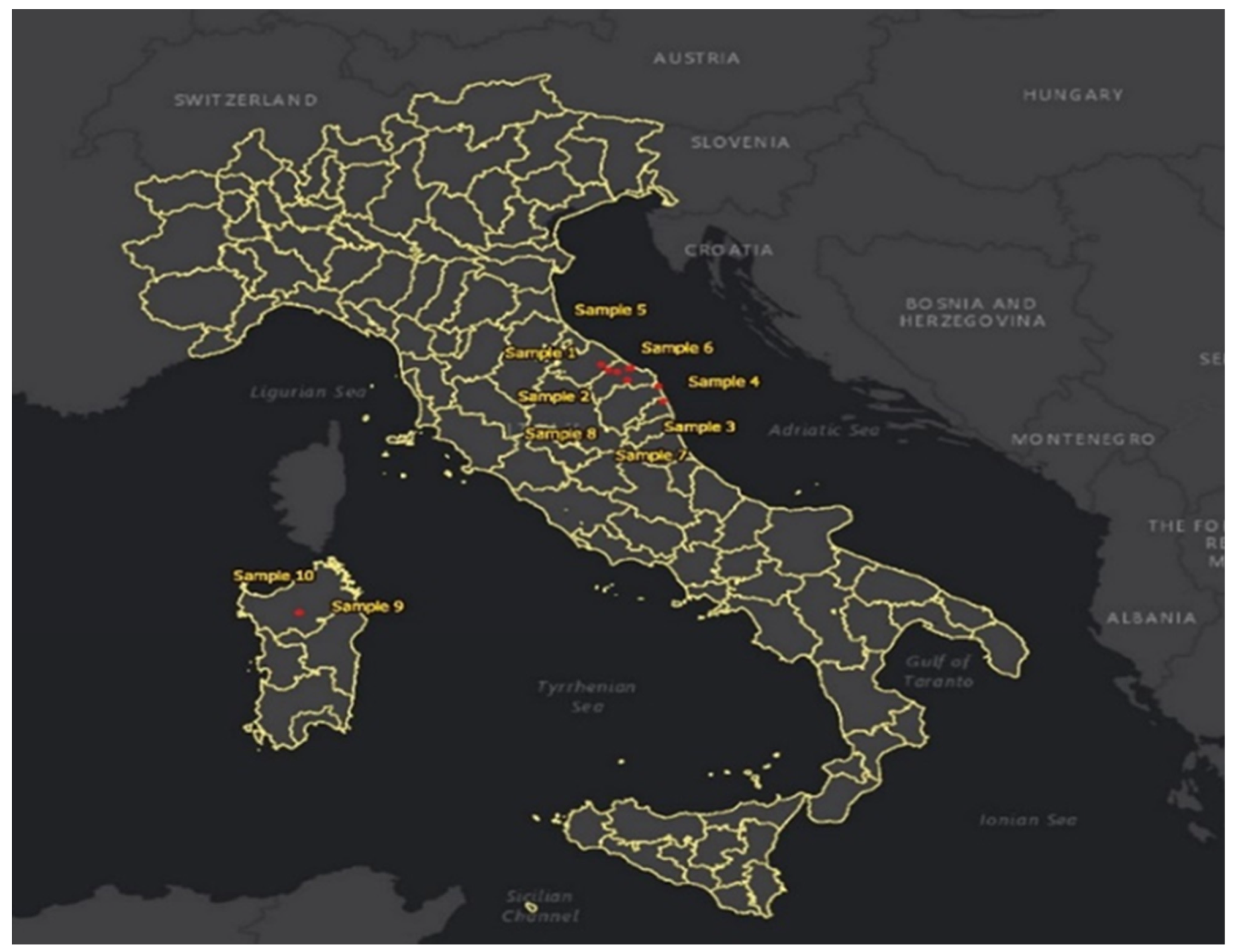
In total, 10 sites (shown in Figure 1) in two Italian regions were visited during the fieldwork campaign that started on the 23 September and ended 20 October 2018. This included two sites in northern Sardinia and eight sites in the province of Marche, which is situated centrally in Italy on the Adriatic coast. Generally, it has a Mediterranean climate with hot, dry summers and cool, wet winters. However, the Italian climate is much more diverse. The most prevalent Köppen climate zones are humid subtropical climates (Cfa), hot-summer Mediterranean climates (Csa), and oceanic climates (Cfb). According to the Köppen climate classification, it is ‘humid subtropical,’ meaning a temperate, rainy climate with a hot summer. The coldest month averages between 0 °C and 18 °C (temperate), at least one month has averages above 22 °C (hot summer) and four months on average above 10 °C with no significant precipitation differences between seasons. The second region, Sardinia, is the second largest island in the Mediterranean Sea. In Sardinia, there is at least three times as much precipitation in the wettest month of the winter than in the driest month of the summer, which has precipitation of less than 30 mm [21].

2.2. In Situ Measurements

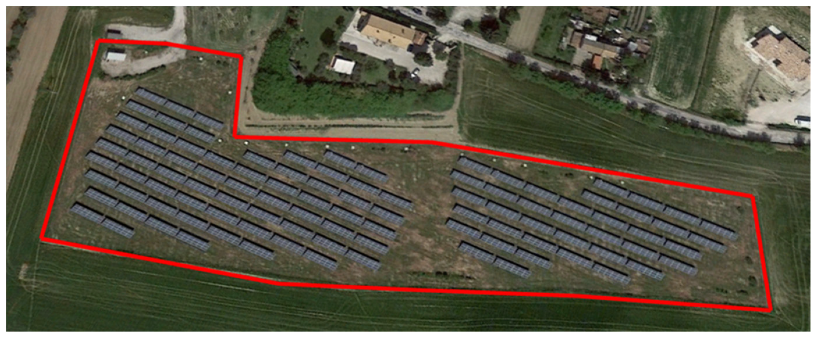
In every park that is visited, four climatological variables are measured, and a vegetation study is performed, as further explained. An example of a park is given in Figure 2. After the vegetation and climatological data are collected, some extra information is gathered for each park. These include a global description of the parks, a description of the overall weather, and a description of the management. Additionally, panel length, panel width, slope, the lowest height of the row, highest height of the row, the width between the rows, and width of the rows are measured.

2.2.1. Micro-Climate

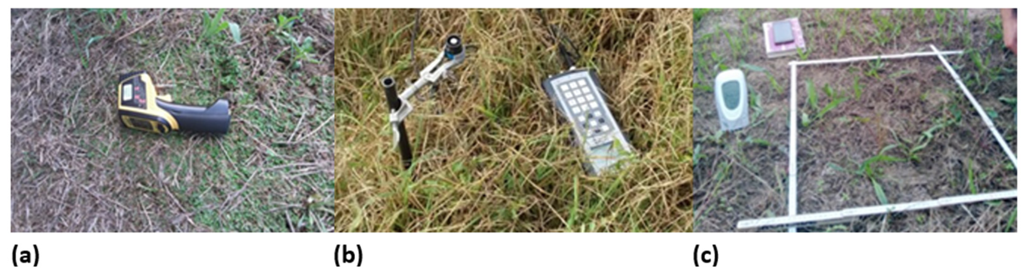
In situ four climatological variables were measured: T_surf, PAR, RH, and T_air. T_air and RH were the standard measurements. PAR was measured to find out how much light is blocked by the solar panels and at a later stage to see if this difference in light can have an impact on biodiversity and vegetation cover. Then the T_surf was measured with a non-invasive dual laser (IR) digital thermometer with a type-K probe of type Traceable^® (VWR International, Leuven, Belgium), shown in Figure 3a. The PAR measurements underneath and between the panels were carried out with a hand-held LI-250A quantum/radiometer/photometer (LI-COR, Inc., Lincoln, NE, USA). The continuous measurements were taken with a LI-1500 light sensor datalogger. Both were connected to an LI-COR quantum sensor of type LI-190R-BNC-2. The LI-1500 light sensor datalogger (right) connected to the quantum sensor (left) is shown in Figure 3b. And Tair and RH were measured with a normal household device, as shown in Figure 3c.

The measurements are taken twice in each park. First, random points were chosen on a map. Then, as shown in Figure 3c, plots of 0.5 × 0.5 m² were taken in five different positions, four positions in the function of the solar panel, and one plot away from the solar panels, but inside the fence of the park, having the same vegetation management. The four positions are always at one-quarter and three-quarters of the width of the row of the panels and between panels, respectively. In each of these positions, all the climatological measurements were taken. Only the T_surf was measured four times, once at the beginning of the visit to the parks and once at the end. The PAR was measured with two devices. One device was fixed outside the park, but within the same management; this was a continuous measurement. The second device was mobile and was used to measure in the different plots; the time was always written down for the comparison with the measurements from the first device. T_air and RH were measured together with the vegetation study because the device needed some time to adjust between two measurements to obtain stable measurements.

2.2.2. Vegetation

As with the climatological measurements, the vegetation survey is conducted twice per park in the four positions in function of the solar panel and a reference position outside the park, within the same management. For each plot of 0.5 × 0.5 m², a detailed vegetation survey is conducted. All plant species are identified and named, and the percentage of coverage of each species is estimated using the Decimal or the Londo scale, as seen in supporting materials (Appendix A,

Table A1. Decimal or Londo scale for recording coverage in vegetation analysis (Reprinted/adapted with permission from Ref. [107] © 2022 Springer Nature Switzerland AG. Part of Springer Nature [107].

DECIMAL SCALE			Braun-Blanquet Scale
Symbol	Coverage	Supplementary Symbols
1	<1%	= r (raro) = rare, sporadic p (paululum) = rather sparse a (amplius) = plentiful m (multum) = very numerous	+
2	1–3%		1
4	3–5%		2
1	5–15%	1 − = 0.7 = coverage 5–10%
		1 + = 1.2 = coverage 10–15%
2	15–25%
3	25–35%		3
4	35–45%
5	45–55%	5 − = coverage 45–50%
		5 + = coverage 50–55%	4
6	55–65%	(coverage > 5%: abundance not indicated)
7	65–75%
8	75–85%		5
9	85–95%
10	95–100%

The decimal point in the symbols·1,·2 and 4 stands for one of the letters r, p, a, or m.

).

2.3. Data Analysis

2.3.1. Data Pre-Processing and Descriptive Statistics

Before the climatological data (T_surf, PAR, RH, and T_air) were used in the data analysis, all the climatological variables were converted to relative variables using Excel. This was to account for variation due to differences in time and between days. This was performed for each position and for each of the variables as follows:

$$\frac{I_{reference }-I_{position 1-4}}{I_{reference}} with I=T_{surf}, PAR, RH, T_{amb}$$

(1)

To use the vegetation data, the data needed to be converted from the Decimal or Londo scale to percentage of coverage per species. From the percentage of coverage per species per plot, the species diversity was calculated by using indices divided into two classes: (1) species richness: “number of species in a community, in a landscape or marinescape, or in a region” [22], which is the most straightforward and simplest method [23,24], and (2) species diversity: which is a combination of species richness and evenness. Evenness is defined as: “the degree to which relative abundances of individuals among the different species are similar for monitoring the biodiversity,” measured by calculating the Shannon diversity index and the Shannon evenness index [25]. The Shannon indices thus combine richness and evenness, but Shannon Diversity emphasizes on richness, while Shannon evenness emphasizes on evenness [26]. The formulas for calculating the different inices are given below. The Shannon evenness index gives the relative evenness, because it divides the Shannon diversity by the natural logarithm of species richness.

$$\mathrm{Species} \mathrm{richness} (S)\text{:} \mathrm{the} S=\sum n$$

(2)

where n = number of species.

Shannon diversity index (H’):

$$H^{\prime }=-\sum _{i=1}^S{p}_i\ln p_i$$

(3)

$$p_i=proportion of individuals of species i usually with 1.5<H^{\prime }<3.5$$

Shannon evenness index (E):

$$E=\frac{H^{\prime }}{{H^{\prime }}_{max}}= \frac{{\sum }_{i=1}^S{p}_i\ln p_i}{\ln S}$$

(4)

with H′_max = S and 0 < E ≤ 1.

For vegetation data, no relative indices are calculated.

To test for normality, the Shapiro-Wilk normality test was performed for all the variables for each position, using Rstudio [27]. For convenience, the outputs are not given. Most of the data were normally distributed, so in these cases the paired t-test could be performed. However, for some variables, the p-values were smaller than 0.05, thereby rejecting the null-hypothesis of normality. This was the case for ‘species richness’ and ‘Shannon diversity,’ so for these two variables, the Mann-Whitney-Wilcoxon test was used.

For both tests, the hypotheses are the same. The null hypothesis (H₀) is as follows: the two samples come from the same underlying populations, or, in other words, they are not significantly different. If the p-value of this test is smaller than α = 0.05, than H₀ will be rejected and the alternative hypothesis will be chosen. The alternative hypothesis (H_A) is as follows: the two samples do not come from the same underlying populations, or, in other words, the two samples are significantly different from each other. Or for this data, that there are significant differences for the climatological variables, between the different positions. The paired t-tests were performed in Excel and the Mann-Whitney-Wilcoxon tests were performed in Rstudio. When the Mann-Whitney-Wilcoxon test was used, this is indicated with an asterix ‘*’ in the Tables. For the climatological variables, six tests could be performed for the combination of the following positions: ‘1–2’, ‘1–3’, ‘1–4’, ‘2–3’, ‘2–4’, and ‘3–4’. For the vegetation data, there were ten tests: the previous six combinations and the combinations: ‘1–5’, ‘2–5’, ‘3–5’, and ‘4–5’.

2.3.2. Linear Mixed-Effects Model

Because the gathered data are of multivariate form with both a fixed variable and random factors, linear mixed-effects models (LMMs) are a good place to start the analysis of the correlated data [28]. Fitting LMMs using Rstudio software (Opensource) [27] can be performed using a large number of packages. In this study, the package ‘nlme’ [29] is used.

As with all coding in Rstudio [27], first the pre-processed dataset is uploaded in the right format. Second, ‘region’ and ‘site’ are defined as factors. Then, a LMM is defined using the ‘lme’ command that is part of the ‘nlme’ package [29]. The code for T_surf (ST) is as follows: lme(ST~P, data = S, random = ~1|R/SI). This means that ST will be predicted in function of the ‘position’ (P). The dataset that is used is defined in Rstudio as ‘S’ and there are two random factors: the first is ‘region’ (R) and within the region, there is the random factor ‘site’ (SI).

2.3.3. General Additive Mixed Model

The second model that was predicted using Rstudio [27] was the general additive mixed model (gamm). This is a non-linear method which predicts the model step-by-step and is better suited for smaller datasets and hierarchical structures [30]. As with the LMM, the datasets are uploaded, the factors are defined after which the gamm is defined using the ‘gamm’ command from the ‘mgcv’ package [29,31,32,33,34,35]. Another important difference with the ‘lme’ command is that ‘gamm’ does not work when missing values (NAs) are present, so an extra command is needed to cope with NAs. The code for this model, for the case of T_surf is as follows: gamm(ST~P, data = S, random = list(R = ~1,SI = ~1), na.action = na.exclude). The same command is also used for the other climatological values and vegetation indices. T_surf (ST) is predicted in function of ‘position’ (P). The variables are in dataset ‘S,’ the random variables are ‘region’ and ‘site,’ and NAs are just excluded from the dataset using ‘na.action = na.exclude.’ Similarly to the ‘lme’ model, a summary is produced that will be analysed and explained in Section 3.

2.3.4. Multidimensional Functional Diversity (FD)

To calculate multidimensional functional diversity indices, two datasets are needed: [species × bioindicators] and [plot × species] [36]. The first is the [species × bioindicators] matrix which gives the bioindicator values for all plant species for the seven different bioindicators: ‘light regime,’ ‘temperatures,’ ‘continentality of the climate,’ ‘humidity,’ ‘acidity or reaction,’ ‘nutrient availability,’ and ‘salt concentration.’ This means that for every plant species that was found in the vegetation analysis and named, those seven values are needed. This was performed by using the list of bioindicator values of vascular plants of the Flora of Italy by Pignatti et al. [37], supplemented with the Ellenberg indicator values of the British countryside by Hill et al. [38]. Available values are not yet for every reported species; from the 96 species, 16 were not specified enough to find values.

The multidimensional diversity indices are then calculated using the ‘dbFD’ command from the stand preference package ‘FD’ [36,39]: dbFD(pign2, tveg, corr = c(”cailliez”)). The Cailliez correction method was used, because ‘sqrt’ did not work [40]. This gives a summary list of nine different indicators and values, but only the last index: the community-level weighted trait means (CWM) will be analysed and used in further analyses. The CWM consists of values for each bioindicator for each community. These values are then used for further preliminary analysis and modelling to see which bioindicators have the most significant differences between communities and thus are affected most by the presence of PV solar panels.

2.4. LU Impact Assessment

The LU impact assessment was conducted utilizing a new method that addresses some earlier problems of the LU impact category of LCIA in agriculture and forestry. These problems were as follows: lack of universal applicability, time/space issues, and arbitrary choice of indicators, among others. The new method was proposed and validated by Peters et al. [19] and is based on ecosystem thermodynamics. They hypothesized that all ecosystems try to control the incoming and outgoing energy flow and try to maximize their internal exergy level when human LU impacts are absent. They measure LU impact as the difference of LU with the reference situation, which is the site-specific maximum ecosystem exergy performance. The method of Peters et al. [19] works by estimating 17 quantitative indicators, which are combined into four thematic scores. These scores are then multiplied by ‘time x area.’ The calculated measure gives the area that is needed for the production of 1 FU in one rotation period [41].

LU impacts can affect the ecosystem quality in two ways. An exergy storage level or the ability to control exergy fluxes can be changed directly (e.g., clipping or harvesting biomass), or indirectly by a change in site quality (e.g., by using fertilizers or irrigation). These changes can lead to another type of climax situation with a different maximum exergy level. The indicators were chosen so that the reference could be placed at the zero point. Impact results were considered as a positive value so that anthropogenically modified ecosystems would obtain positive impact scores. However, there are cases in which a negative impact score is possible (e.g., introduction of a new species that increases the buffering capacity without changing the quality of the ecosystem) [41].

The four thematic scores are as follows: (1) S: soil and nutrients, (2) W: water, (3) V: ecosystem biomass and structure (vegetation), and (4) B: biodiversity. The aggregated thematic scores are given by four formulas:

$${\mathsf{\Delta }\mathrm{Q}}_S=\frac{{\sum }_{i=1}^n{\mathsf{\Delta }\mathrm{Q}}_{Si}}{N} where N=5$$

(5)

$${\mathsf{\Delta }\mathrm{Q}}_V=\frac{{\sum }_{i=1}^n{\mathsf{\Delta }\mathrm{Q}}_{Vi}}{N} where N=5$$

(6)

$${\mathsf{\Delta }\mathrm{Q}}_W=\frac{{\sum }_{i=1}^n{\mathsf{\Delta }\mathrm{Q}}_{Wi}}{N} where N=2$$

(7)

$${\mathsf{\Delta }\mathrm{Q}}_B=\frac{{\sum }_{i=1}^n{\mathsf{\Delta }\mathrm{Q}}_{Bi}}{N} where N=5$$

(8)

These scores can then be divided in two groups: (1) to reflect the buffering capacity (soil and water), and (2) to reflect the exergy level of the ecosystem (vegetation and biodiversity) [41]. However, they need to be adjusted for time and area by multiplying with ‘time × area’ (‘0.6667 ha × 1 year’):

$$S_i={\mathsf{\Delta }\mathrm{Q}}_i\ast {\left(area\ast time\right)}_{FU}\ast F{U}^{-1} for$$

(9)

$$i=soil, water, vegetation and biodiversity$$

Before being able to calculate all these indicators, scores, and impacts, an LCI analysis needs to be performed. This step is very resource- and time-intensive with constraints on the data collection [42]. This method is used to compare a solar park versus intensive agricultural land use. The idea was to perform this test twice. One time for each test site: Marche and Sardinia. However, the goal of this approach is not to have a detailed comparison of two land use types, but more to have an idea of the order of magnitude or an overall picture of the most important differences between the two land use types and their deviations from the natural case. The data come from different sources, with small differences in the type of soil, vegetation, time of the year, etc. Using a pragmatic engineering approach, the test is therefore only performed once without making a meticulously accurate description of the climax vegetation using the Natura 2000 habitat types [43,44]. All the references are given in Appendix C,

Table A3. Table with references for the gathered information that is needed to perform the land use impact assessment.

Indicator	Variable	References
Soil compaction	Areaaff/tot/ * Permeabilityaff/ref	[89,90,91]
Soil disturbance	Areaaff/tot/depth/ times/rot length	[47,68]
Soil erosion	USLE/depth	[48,49]
CEC	* CEC	[50,51,111]
BS	* BS	[52,53,112]
Evapotranspiration	* ET	[53,54,55]
Surface runoff	SR/P/ET	[57,58]
TAB	* TAB	[58,59,60]
LAI	* LAI	[60,61,62]
fNPP	* NPP	[59,60,63]
Crop biomass	Crop and total biomass	[65]
Vegetation Height	Heightact/ref	[65,66]
Water balance	Areairr/drain/tot	[68]
Fertilization /impoverishment	Areaaff/tot/times/ rot length	[68]
Biocides	Areaaff/tot/times/ rot length	[68,98]
Exotic plant	Coverexot/tot	[101,104]
Species	* Sp	[101,102,103]

All these variables are needed for both the intensive agriculture and the solar park for both habitat types. When the variables are indicated with ‘*’ the reference value for the climax vegetation is needed.

.

3. Results

3.1. Preliminary Results

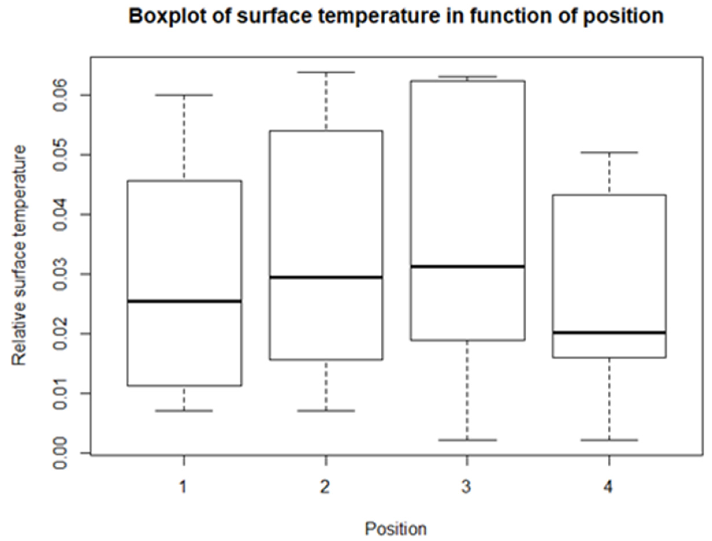
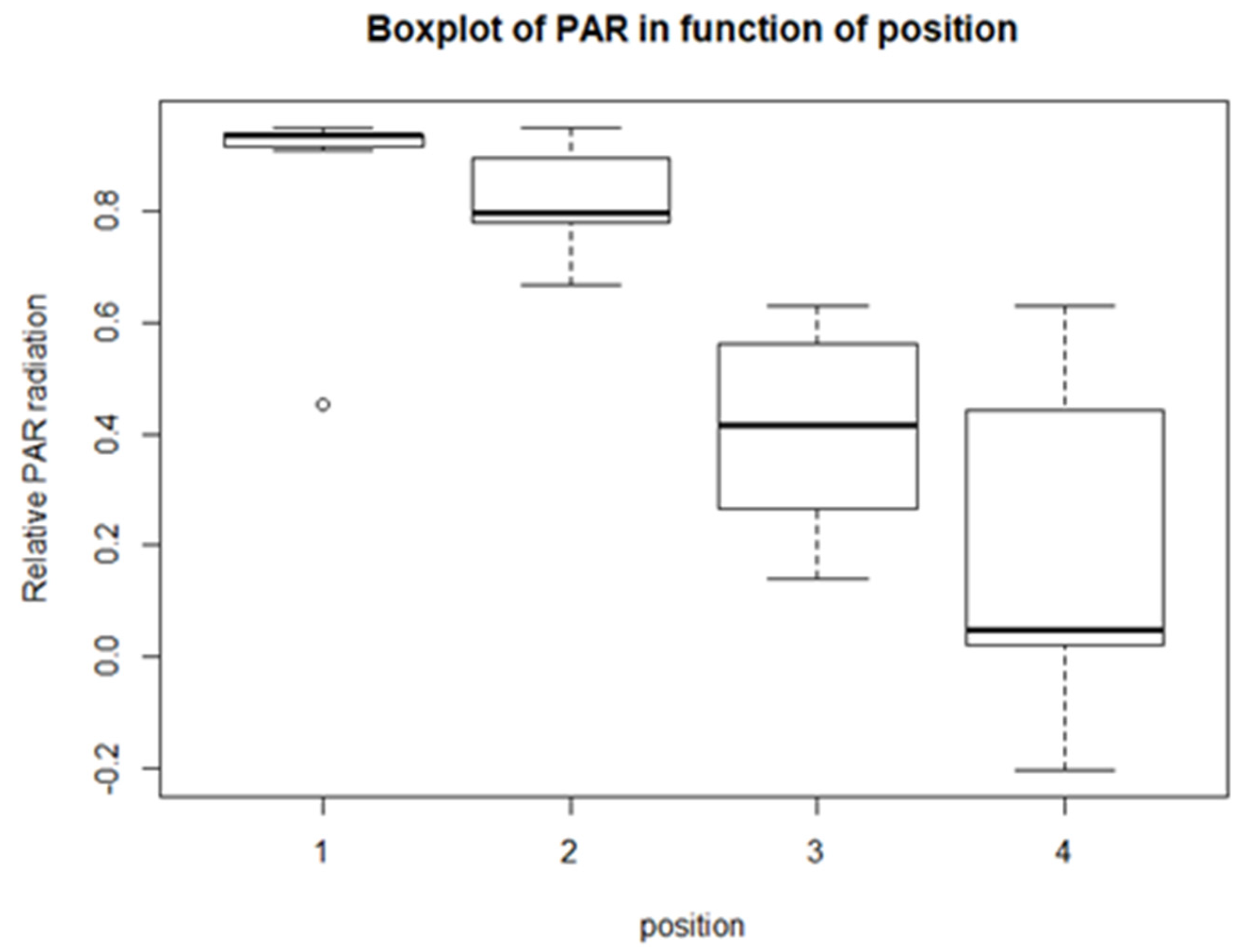
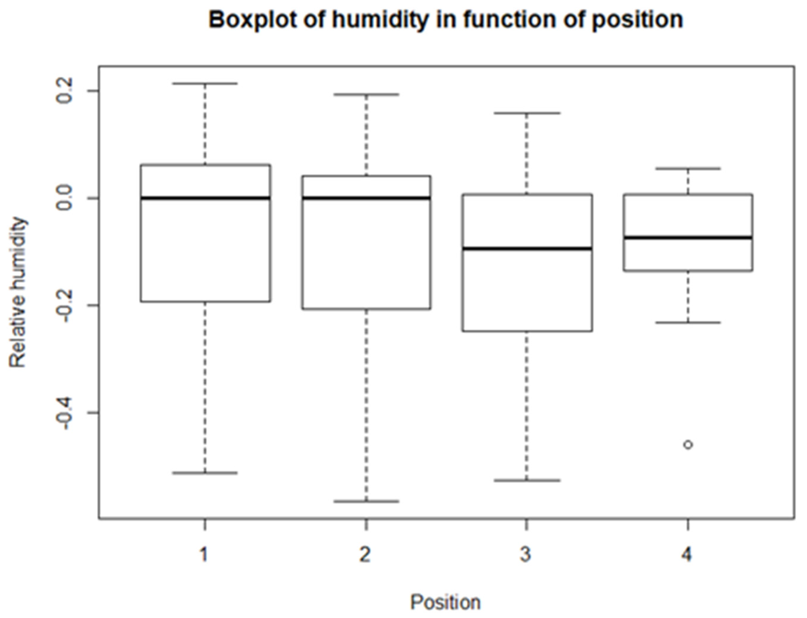
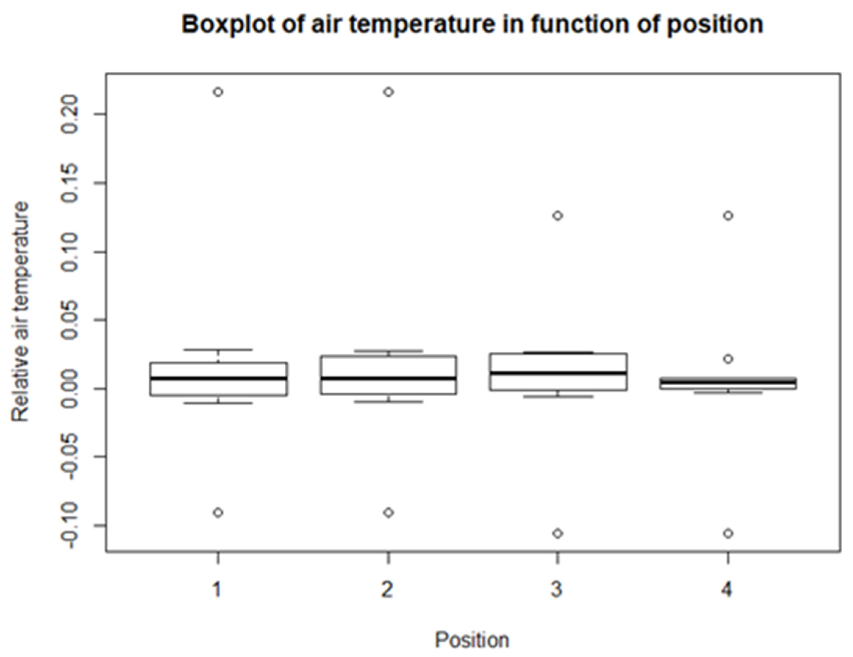
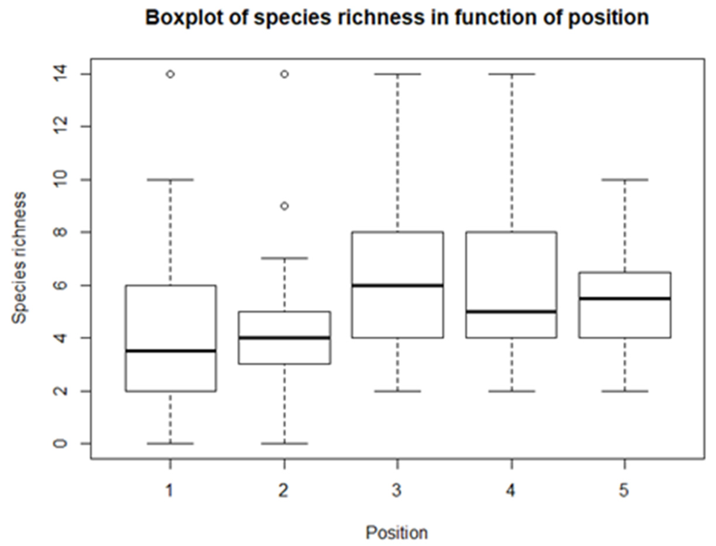
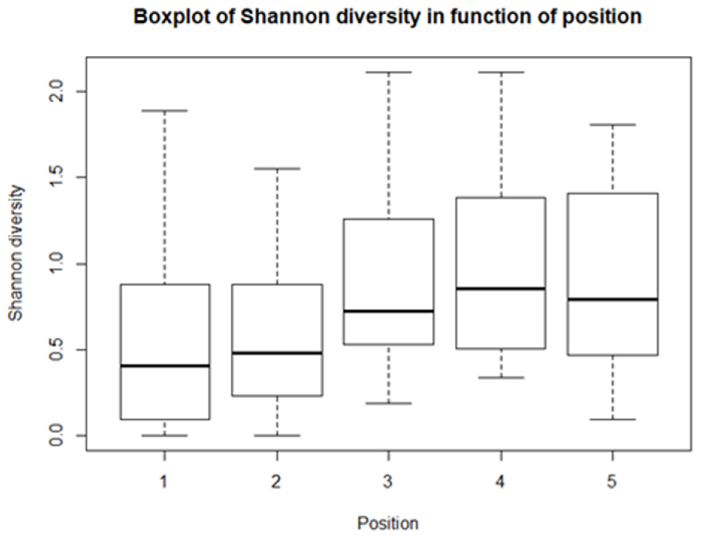
From the descriptive statistics, there are some preliminary results. For each of the climatological variables, T_surf, PAR, RH, and T_air, a set of boxplots is given. The boxplots give their calculated values in function of their position in relation to the solar panel. The boxplots are shown in Figure 4, Figure 5, Figure 6 and Figure 7. Figure 4 shows the boxplots for T_air; it looks as though there is a gradient with the highest relative temperatures on positions 2 and 3, but with large variations. Figure 5 shows the boxplots for PAR; again, there is a gradient which goes from the highest relative radiation on position 1 to the lowest relative radiation on position 4. There is also a lot of variation, especially for positions 3 and 4. Figure 6 shows the boxplots for RH; here there is no clear gradient, although the average relative RH is lowest on position 3, and also the average relative RH of position 4 is lower than those of 1 and 2. Lastly, from the boxplots for T_air, it is very difficult to make general observations, because there are a lot of outliers in both directions. Additionally, for the vegetation indices, species richness, Shannon diversity, and Shannon evenness, there are some preliminary results. The first boxplot shown in Figure 8 shows the species richness in function of position. It looks as though the average species diversity is lower under the solar panels than between the rows or outside the park. However, as with the climatological data, there is quite a lot of variation between sites; this is also true for Shannon diversity and Shannon evenness. Figure 9 shows the Shannon diversity in function of position. The pattern is similar to that of species richness; the diversity is lower underneath the panels than between the panels and outside the park.

Table 1. p-values of the paired t-tests between the different positions for the four climatological measurements.

The t-Test between Position:	Surface Temperature	PAR Radiation	Humidity	Air Temperature
1 and 2	0.023	0.37	0.067	0.27
1 and 3	0.021	0.0011	0.0076	0.19
1 and 4	0.33	0.00043	0.094	0.42
2 and 3	0.20	8.0 × 10−6	0.026	0.23
2 and 4	0.066	5.6 × 10−5	0.20	0.30
3 and 4	0.036	0.015	0.48	0.15

gives the p-values of the paired t-test between the different combinations of positions for the climatological variables. For T_surf, there are significant differences for combinations ‘1–2’, ‘1–3’ and ‘2–4’. For PAR, in all but one (‘1–2’) of the combinations, they are significantly different. For RH, combinations ‘1–3’ and ‘2–3’ are significantly different. And for T_air, there are no significant differences between positions.

Table 2. p-values of the paired t-tests between the different positions for the three vegetation indices. Indices indicated with ‘*’ have a non-normal distribution, so their difference is tested with the Mann-Whitney-Wilcoxon test, instead of the paired t-test.

t-Test between Position:	Species Richness *	Shannon Diversity *	Shannon Evenness
1 and 2	0.73	0.56	0.37
1 and 3	0.035	0.012	0.0070
1 and 4	0.032	0.0079	0.0018
1 and 5	0.091	0.019	0.0030
2 and 3	0.044	0.030	0.021
2 and 4	0.041	0.012	0.0097
2 and 5	0.076	0.040	0.025
3 and 4	0.99	0.91	0.22
3 and 5	0.53	0.80	0.52
4 and 5	0.73	0.88	0.88

gives the p-values for the 10 different combinations of positions for the vegetation indices. For species richness, there are four combinations which are significantly different: ‘1–3’, ‘1–4’, ‘2–3’, and ‘2–4’. For Shannon diversity, six combinations are significantly different from each other: ‘1–3’, ‘1–4’, ‘1–5’, ‘2–3’, ‘2–4’ and ‘2–5’. The same combinations are significantly different for Shannon evenness.

3.2. Linear Mixed-Effects Model

For the first model, both the p-values of the intercept and position are bigger than the significance level of 0.05 (

Table 3. Output of the linear models fitted in R.

Linear Model		Value	Std. Error	DF	t-Value	p-Value
Tsurf~P	Intercept	0.02658	0.01367	29	1.945	0.06150
	Position	−0.0007015	0.001055	29	−0.6647	0.5115
PAR~P	Intercept	1.260	0.1265	26	9.961	0
	Position	−0.2530	0.02640	26	−9.584	0
RH~P	Intercept	−0.04684	0.07073	26	−0.6623	0.5136
	Position	−0.01758	0.007366	26	−2.386	0.02460
Tair~P	Intercept	0.02772	0.02400	26	1.155	0.2585
	Position	−0.005171	0.002581	26	−2.003	0.0557
S~P	Intercept	4.530	1.419	97	3.193	0.001900
	Position	0.4475	0.1824	97	2.453	0.01590
H’~P	Intercept	0.5011	0.2700	97	1.856	0.06650
	Position	0.1201	0.02642	97	4.548	0
E~P	Intercept	0.4941	0.3776	96	1.308	0.1939
	Position	0.09149	0.01967	96	4.652	0

). This means that there is not enough evidence for a linear relationship between T_surf and position. This is also the case for T_air, although only barely. For all the other lme models, there is a significant linear relationship. For PAR, there is a very strong negative linear correlation. There is also a negative linear relation for RH, but with a rather small coefficient. For the vegetation indices, there is a significant positive linear relationship between the de indices and the position. Species richness, Shannon diversity, and Shannon evenness increase from position 1 to position 5.

3.3. General Additive Mixed Model

The first things that stand out in

Table 4. Output of the generalized additive mixed models fitted in R.

Gamm		Value	Std. Error	t-Value	p-Value	R-sq (adj)
Tsurf~P	Intercept	0.02912	0.009155	3.181	0.00292	−0.0247
	Position	−0.0007015	0.001064	−0.6590	0.5140
PAR~P	Intercept	1.253	0.1024	12.24	5.23 × 10−14	NA
	Position	−0.2530	0.02677	−9.450	4.86 × 10−11
RH~P	Intercept	−0.04684	0.06881	−0.6810	0.5010	NA
	Position	−0.01758	0.007438	−2.363	0.024
Tair~P	Intercept	0.02772	0.02335	1.187	0.2434	NA
	Position	−0.005171	0.002606	−1.984	0.0554
S~P	Intercept	4.400	1.054	4.174	6.14 × 10−5	0.0256
	Position	0.4456	0.1832	2.433	0.01670
H’~P	Intercept	0.04673	0.1912	2.443	0.0162	0.0819
	Position	0.1199	0.02653	4.521	1.61 × 10−5
E~P	Intercept	0.4888	0.2724	1.794	0.0756	NA
	Position	0.09141	0.01975	4.628	1.06 × 10−5

are the adjusted R² values. In four of the seven cases, they are missing, and they are very low for the three other models. The models for T_surf and T_air are not significant. For all the other models, they are significant. To see if these models have more information about the data, they were plotted for simplicity, but these plots were not shown, as explained further in Section 4.

3.4. Multidimensional Functional Diversity Indices

Table 5. Output of the linear models from the CWM indices fitted in R.

Linear Model		Value	Std. Error	DF	t-Value	p-Value
Light~P	Intercept	7.719	0.8910	87	8.664	0
	Position	0.1462	0.04946	87	2.956	0.004000
Temp~P	Intercept	6.629	0.2924	87	22.67	0
	Position	0.09673	0.05326	87	1.816	0.07280
Cont~P	Intercept	5.080	0.2162	87	23.49	0
	Position	0.0003660	0.03171	87	0.01153	0.9908
Hum~P	Intercept	4.803	0.2204	87	21.79	0
	Position	−0.08587	0.06156	87	−1.395	0.1666
Reaction~P	Intercept	5.762	0.2481	87	23.22	0
	Position	0.2085	0.06884	87	3.028	0.0032
Nutrients~P	Intercept	6.629	0.7782	87	8.518	0
	Position	−0.2438	0.05757	87	−4.235	1 ×10−0.4
Salt~P	Intercept	0.2916	0.1606	87	1.816	0.0729
	Position	−0.03602	0.01778	87	−2.026	0.04580

gives the models of the CWM indices. All the intercepts have p-values smaller than the 0.05 significance level, except for the intercept of ‘salt.’ For position, there are fewer models with p-values smaller than the 0.05 significance level. Thus, not all models have enough evidence for linearity. The models that do have evidence for linearity are ‘light,’ ‘reaction,’ ‘nutrients,’ and ‘salt.’ The reason for this will be explained further in the ‘Discussion’ section.

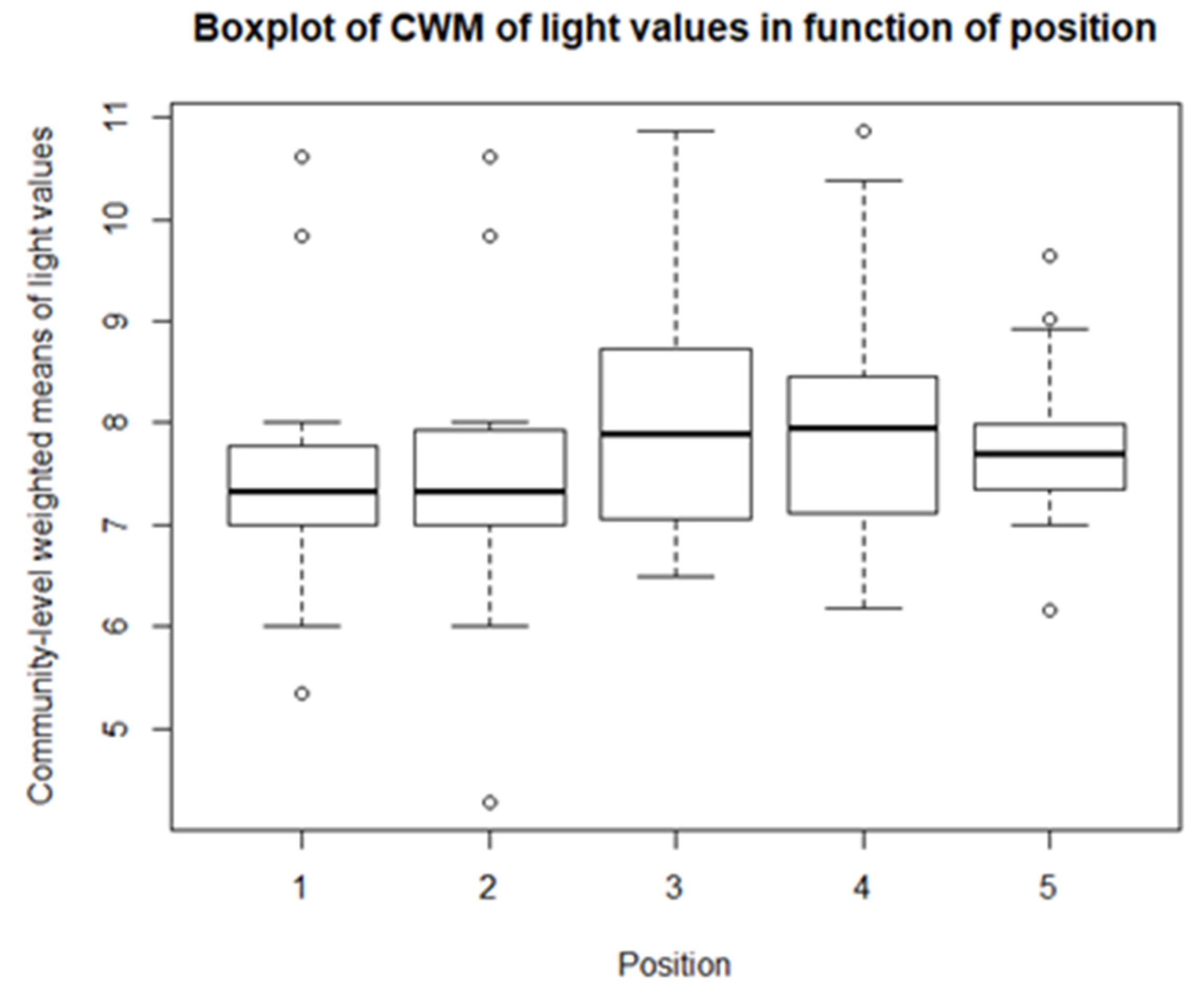
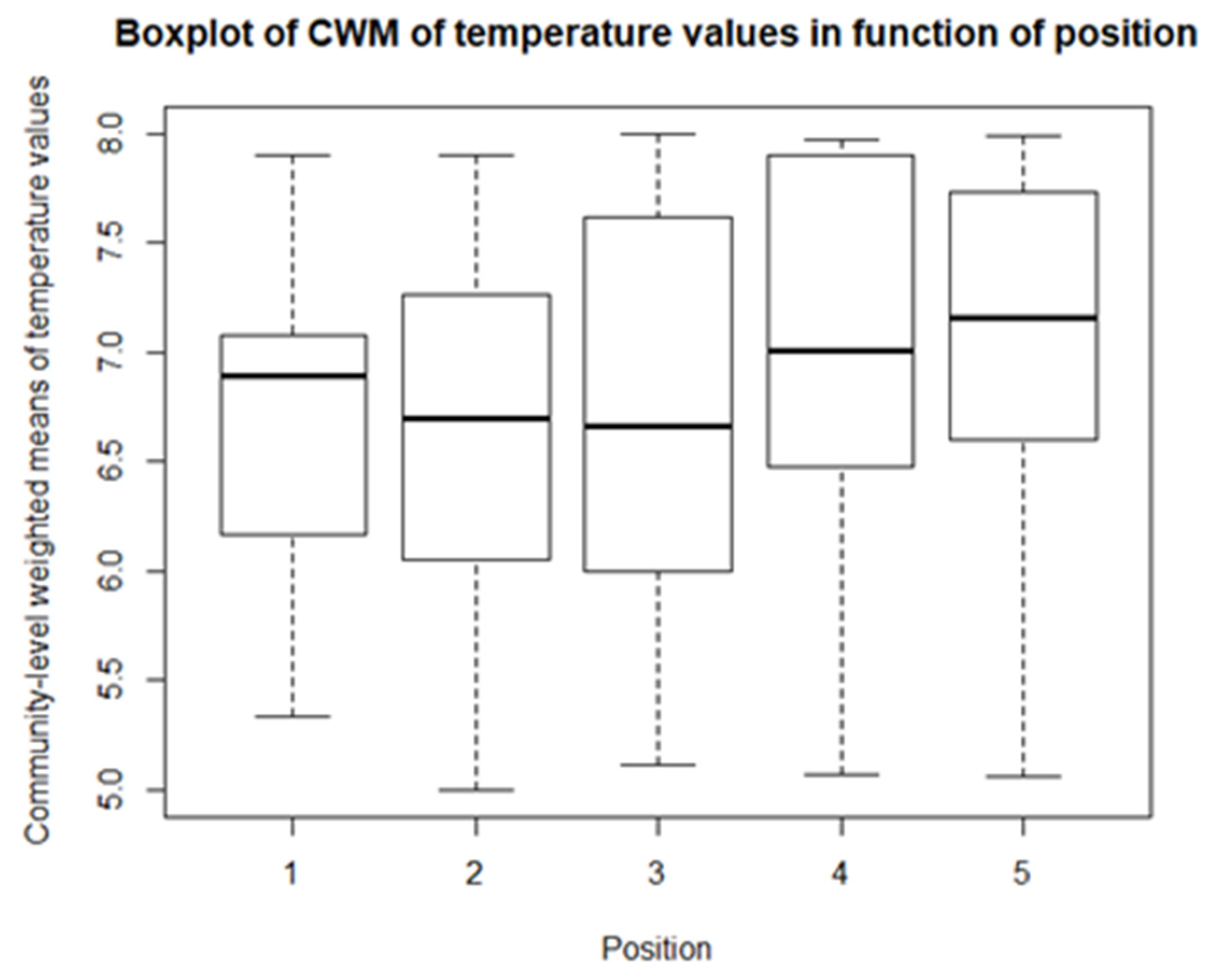
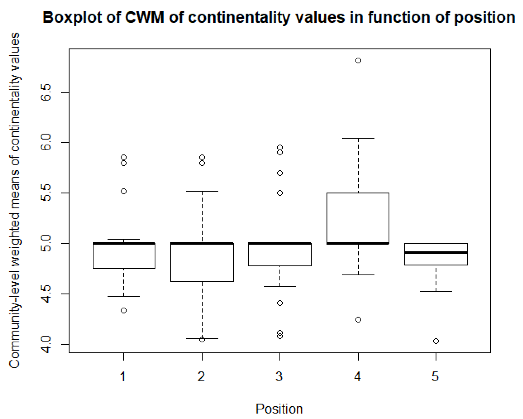
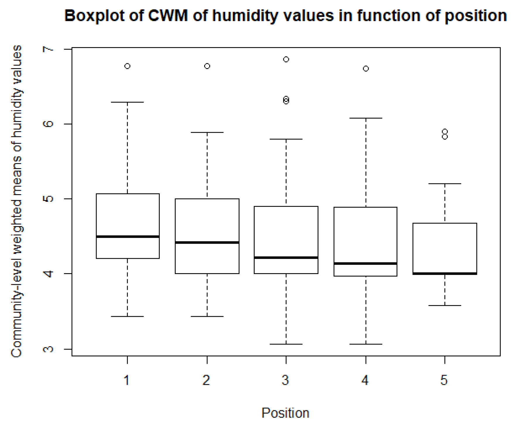
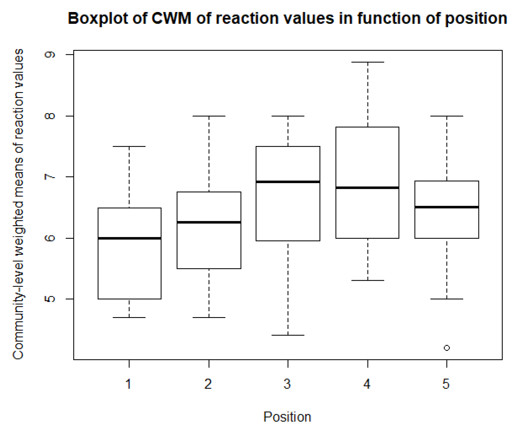
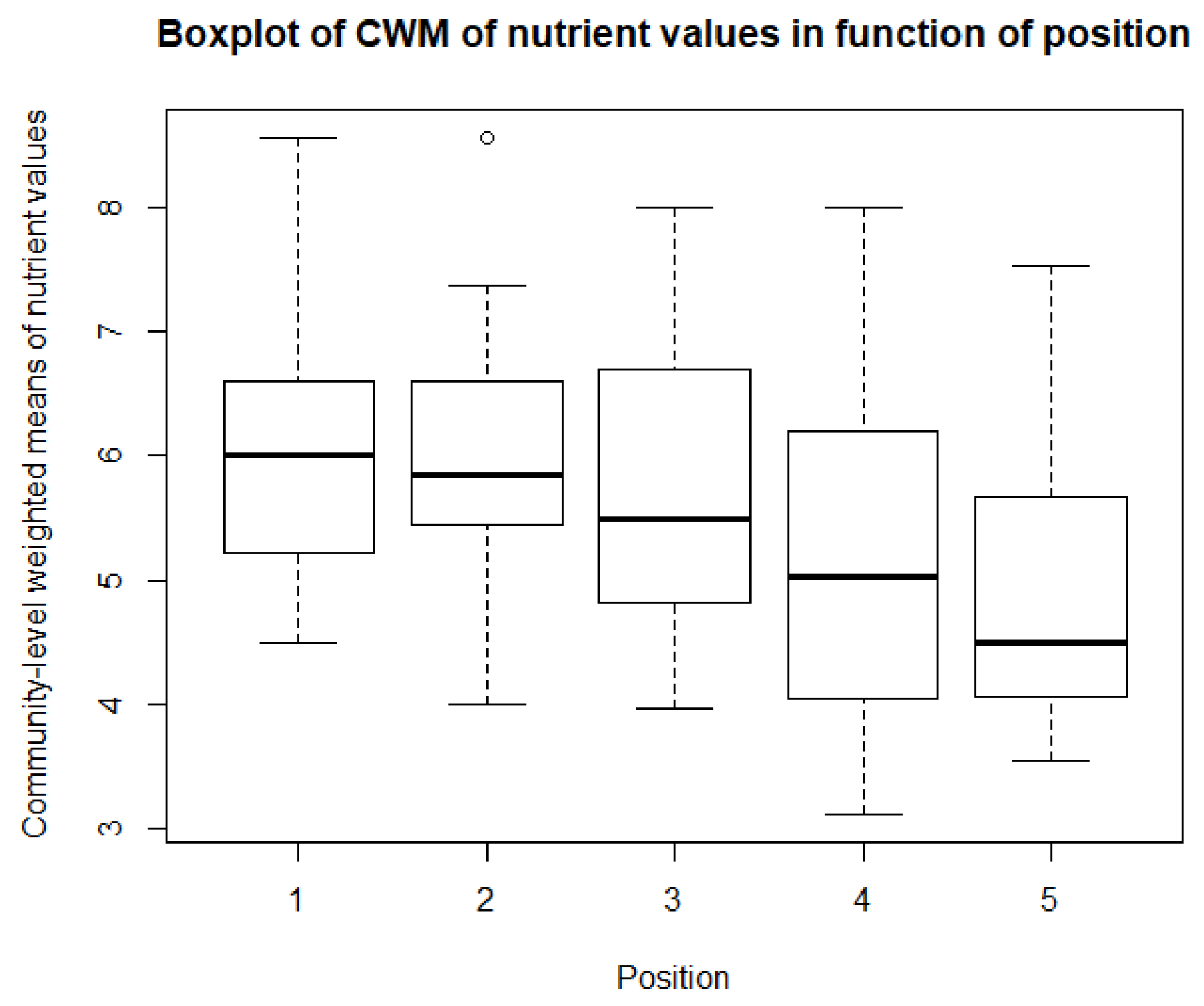
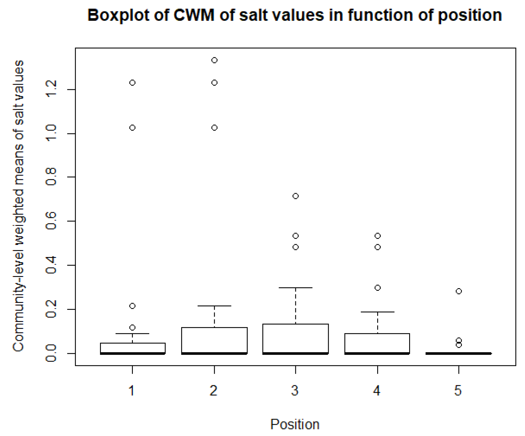
As for the climatological variables and vegetation indices, some descriptive statistics are performed for the CWM values. These include boxplots and paired t-tests, or Mann-Whitney-Wilcoxon tests in the case of non-normality. So, for each of community, there is a boxplot made of the community-weighted trait means mean values. So, for each bioindicator, there are five boxplots, with one for each position. The first boxplots are for the light regime and are shown in Figure 10. The average light regime values are between 7 and 8. It seems that for the positions under the panels, the light regime values are slightly lower values than those between the panels and outside the park. However, there is also more variation in the values for the positions between the panels. For the values of temperature, shown in Figure 11, the minimum and maximum values are the same for each position. It appears that the values of position 2 and 3 are lower than those of the other three positions. The values for the continentality of the climate have one-sided boxplots with a lot of outliers, which can be seen in Figure 12. The averages then are practically the same, except the average of position 5 is slightly smaller. The fourth bioindicator, humidity, is shown in Figure 13. These have almost the same spread for each position, but there looks to be a small downward trend from position 1 to position 5. There are also some outliers at the high end of the boxplots. Figure 14 shows the boxplots for acidity or reaction. The lowest averages are found for position 1 and the highest for position 3. There seems to be a positive relation from position 1 to position 3, and from there on, downward to position 5. The second to last set of boxplots given in Figure 15 are for the values of nutrient availability. Here the trend is the clearest. It is downward with the highest average for position 1 and the lowest for position 5. The last set of boxplots are for salt concentration and are shown in Figure 16. These are also one-sided boxplots with averages of a little more than 0 and the most variation for position 3.

For the bioindicators of ‘continentality of the climate,’ ‘reaction,’ and ‘salt concentration,’ the distribution was not normal, so instead of the paired t-test, the Mann-Whitney-Wilcoxon test were performed. The p-values of these tests are given in

Table 6. p-values of the paired t-tests between the different positions for the CWM values of the different bioindicators. CWM values indicated with ‘*’ have a non-normal distribution, so their difference is tested with the Mann-Whitney-Wilcoxon test, instead of the paired t-test.

t-Test between Position	Light	Temperature	Continentality *	Humidity	Reaction *	Nutrients	Salt *
1 and 2	0.74	0.60	0.82	0.29	0.35	0.73	0.78
1 and 3	0.24	0.60	0.84	0.71	0.027	0.14	0.76
1 and 4	0.36	0.28	0.19	0.60	0.010	0.017	1
1 and 5	0.48	0.33	0.32	0.32	0.10	0.00059	0.31
2 and 3	0.0028	0.68	0.68	0.86	0.16	0.43	0.98
2 and 4	0.014	0.14	0.14	0.73	0.053	0.031	0.79
2 and 5	0.082	0.13	0.43	0.58	0.42	0.0044	0.22
3 and 4	0.30	0.042	0.26	0.80	0.70	0.0066	0.71
3 and 5	0.39	0.18	0.19	0.47	0.47	0.032	0.16
4 and 5	0.74	0.96	0.0047	0.56	0.34	0.73	0.25

. For light regime, there are only significant differences for the combinations ‘2–3’ and ‘2–4’. For temperatures, there was only one significant difference: ‘3–4’. Additionally, for continentality of the climate, there was only one significant difference: ‘4–5’. For humidity and salt concentration, there were no significant differences. Reaction had three combinations that were significantly different: ‘1–3’, ‘1–4’, and ‘2–4’. And for nutrient availability, they were all significantly different except for the combinations: ‘1–2’, ‘1–3,’ ‘2–3’, and ‘4–5’. Further explanation is given in the Section 4.

3.5. LU Impact Assessment

The LU impact assessment was performed for a Mediterranean climate. All values for the 17 indicators, the division in themes, and the land use scores for these themes are given in

Table 7. The individual scores for each indicator for the wheat field and the solar park (grassland). And the total LU for the production of 1 FU for each thematic scores for a wheat field and a solar park (grassland) [(ha × yr)/FU].

	Wheat	Solar	Land Use	Wheat	Solar
Soil compaction	91	39	Soil	40	18
Soil structure disturbance	37	0
Soil erosion	100 *	0
Cation exchange capacity	84	30
Base saturation	−13	66
Evapotranspiration	26	3	Water	9	1
Surface runoff	0	0
Total aboveground living biomass	91	96	Vegetation	32	25
Leaf area index	9	0
Free net primary production	26	0
Crop biomass	26	0
Vegetation height	89	90
Artificial change in water balance	100	0	Biodiversity	31	15
Liming, fertilisation, impoverishment	100 *	0
Biocides	100 *	0
Canopy cover of exotic species	1	46
Number of species	94	65
Total	961	435
Average	56.5	25.6

* The values are cut off at the maximum value of 100.

. For each theme, some things stand out. For ‘soil,’ all indicator values, except the indicator for ‘base saturation’ are higher for the wheat field than for the solar farm. The overall land use score is thus also higher. For ‘water,’ there were no accurate data for ‘surface runoff,’ and again the value for the other indicator and the overall land use is higher for the wheat field. For ‘vegetation,’ the land use of a wheat field is slightly worse. A wheat field performs worse (highest values) for ‘leaf area index,’ ‘free net primary production,’ and ‘crop biomass.’ They perform approximately the same for the other two indicators. The last theme is ‘biodiversity,’ in which the land use score is also higher for a wheat field compared to a solar park. The wheat field performs worse for all indicators, except for ‘canopy cover of exotic species.’ Overall, the wheat field is worse than the solar park, so the overall land use for a wheat field is higher compared to the solar park.

Three values are indicated with *; this means that they exceed the maximum of 100. Therefore their values are changed to this cut-off value of 100 [41].

The papers used to calculate the indicators are as follow: [45,46,47] for ‘soil compaction,’ [48] for ‘soil structure disturbance,’ [48,49,50] for ‘soil erosion,’ [51,52] for ‘cation exchange capacity,’ [52,53] for ‘base saturation,’ [54,55,56] for ‘evapotranspiration,’ [57,58] for ‘surface runoff,’ [59,60,61] for ‘total aboveground living biomass,’ [61,62,63] for ‘leaf area index,’ [60,61,64] for ‘free net primary productivity,’ [65] for ‘crop biomass,’ [66,67] for ‘vegetation height,’ [68] for ‘artificial change in water balance,’ [69] for ‘liming, fertilization and impoverishment,’ [69,70] for ‘biocides,’ [71,72] for ‘canopy cover of exotic species’ and [71,73,74] for ‘number of species.’ This is also given in Appendix C, Table A3.

4. Discussion

4.1. Microclimate and Vegetation

The goal of the research was to increase our understanding of the effect solar panels can have on microclimate and vegetation. The most comparable research that was found was the paper of Armstrong et al. [10]. The paper is called “Solar park microclimate and vegetation management effects on grassland carbon cycling” [75]. A comparison of their research to this research was performed for every variable that was measured or calculated from the measurements.

Before starting the discussion, it is noted that the climatological values are relative values calculated as follows:

Before starting the discussion, it is noted that the climatological values are relative values calculated as Equation (1).

The different positions indicated from 1 to 4 are in function of the position in relation to the solar panels, as can be seen in Figure 8. Position 5 is the reference position outside the park, within the same management.

The first variable is T_surf. The first things that stand out are the low values of relative temperature; they range from just above 0.0 to just above 0.06. This can be explained by the conversion of degrees Celsius to Kelvin, where the numerator is small compared to the denominator. Second: from the boxplots, it is shown that there is an increase in relative temperature from positions 1 to 3 and a decrease to position 4. The t-tests show that there were significant differences in the values of positions 1–2, 1–3, and 3–4, but not for 2–4. This means that the relative surface temperatures of positions 1 and 4 are significantly lower than those of positions 2 and 3, or that the highest surface temperatures are measured on positions 1 and 4. Thus, there is a cooling effect of the solar panels, but only if the panel is high enough above the ground, as is the case at position 2. Additionally, for position 3, the panels can still provide shade, lowering T_surf. This is because of the N-S orientation. Although Armstrong et al. [10] did not measure T_surf, they found that the soil was significantly cooler under the solar panels compared to the situation between rows and the reference outside the park. They only took one measurement in the middle of the row and in the middle between rows. They could not make a distinction between different positions under and between panels, as in this research. The reason why the temperature is lower underneath the panels can be attributed to the interception of shortwave radiation by the PV arrays [76]. Another possible explanation that was considered was the change in albedo. There are two effects: first a warming effect due to a lower albedo (solar panel) and a counteracting cooling effect due to the conversion of heat to energy; the total effect turned out to be negligible [77,78,79]. No model could be predicted with lme, so there is no extra information from linear modelling.

The second variable is PAR. There is a clear negative gradient in relative PAR from position 1 to position 4 which is supported by the t-tests and the lme model. Only for positions 1 and 2 was there not enough evidence that they were significantly different. This outcome was to be expected; the solar panel will block sunlight from reaching the ground and the closer the solar panel is to the ground, the less radiation can reach the ground. High relative PAR values mean a lot of radiation is blocked, which is the case for positions 1 and 2; the least amount is blocked in position 4. This outcome was also found by Armstrong et al. [10] and Tanner et al. [20]. The latter found that the decrease in PAR was up to 85%. Armstrong et al. [10] also made a distinction between direct and diffuse radiation and found that there was more diffuse radiation under the panels compared to between rows, which could be beneficial for vegetation growth. For the linear modelling: the intercept of the lme models is not relevant, because a relative position of ‘0’ does not exist, however when combined with the slope, they could provide additional insight. The intercept is 1.260 and the slope is −0.2530. If one would then calculate the relative PAR for the four positions, almost all sunlight would be blocked on position 1 and each subsequent position has about 25 percent more sunlight. The lower PAR results in lower photosynthesis activity and thus lower biomass under the solar panels. These lower PAR levels could offer the potential for a more diverse plant community with more shade plants underneath and more radiation-tolerant plants between rows and outside the park [80].

The next variable is humidity. There is a lot of spread in the data and both negative and positive values for relative humidity are calculated. The values for relative RH for position 1 and position 2 are the most alike. Those for position 3 are the lowest and are all negative. Additionally, the t-tests show that 3 is significantly different from 1 and 2. This means that the RH is clearly the highest at position 3, directly next to the row, because negative values for relative RH mean that RH in the park is higher than the reference RH outside the park. This is the case for 75% of the measurements that were taken on positions 3 and 4. In general, RH is thus higher between rows than underneath the panels and outside the park. This is also visible from the lme model, which shows a negative relationship. However, the intercept and slope of the model are small compared to the spread of the data, so conclusions must be made carefully. This is not fully in line with the findings of Armstrong et al. [10]. They did not use RH directly, but converted RH to absolute humidity (AH), which is directly correlated with RH and vapour pressure deficit (VPD), which is inversely related to RH. Both measures gave the same result, that the average RH underneath panels was higher than RH between rows and outside the park and from spring to autumn; however, the daily variation was smaller for both, with a higher minimum and lower maximum [10,75]. They attributed these lower daily maxima to lower evapotranspiration rates underneath the panels, and the higher daily average to lower transpiration rates. This is fully in line with the lower photosynthesis rates and plant biomass under the solar panels [75]. The discrepancy between our research and the literature could be because of the adjustment time between two measurements, or because in this research there were only momentary measurements taken on different days and times of days.

The last climatological variable is T_air. The data for this variable show that there are almost no differences between the temperature underneath the panels or between the rows compared to the reference position, because for each position the average is about 0, with some outliers. Additionally, the modelling did not give any more information. Armstrong et al. [10] also found that the average temperatures were not different for the different positions. However, they were able to show that the T_air underneath the panels had smaller variations during the day; this was also found by Tanner et al. [20], who stated that temperatures could be up to 11 °C cooler. T_air was also measured with the device humidity was measured with, so for T_air, the measurements could also be less accurate than expected, due to the adjustment time of the device.

The vegetation indices, species richness, Shannon diversity, and Shannon evenness, all showed approximately the same pattern. For each index, positions 1 and 2 had the lowest values, and 3, 4, and 5 had the highest values. In other words, the richness, diversity, and evenness are all lower underneath the panels than in between the rows and outside the park. This was supported by the t-test (for Shannon evenness) and the Mann-Whitney-Wilcoxon tests (for species richness and Shannon diversity). Additionally, their lme models were significant, meaning that they all had evidence for linearity. This is evidence that solar panels have a negative effect on vegetation. Armstrong et al. [10] also found fewer species and lower biomass in the reference plots and between the rows compared to underneath the solar panels. Probably, the vegetation in these solar parks is native and is adapted to the local climate and the site. The solar panels thus lower incident radiation, lower temperature, and lower rainfall, which will result in a negative impact. Another possible explanation could be a higher maintenance pressure underneath the panels, to make sure the vegetation does not damage the panels, rendering a whole array functionless. Another note that must be made about indices is their value. Shannon diversity is normally between 1.5 and 3.5, or 4.5 in extreme cases. For Shannon evenness, the value cannot exceed 1, so some errors are made during measurements or calculations, resulting in outliers larger than 1. There is however some evidence that largescale installations could have a positive impact on vegetation, especially in very degraded areas, where precipitation is the limiting factor. Large installations can increase temperature and rain, in turn creating better conditions for vegetation, which further enhances precipitation and thus creates a positive feedback loop [81]. Additionally, Norton & Young [82] found evidence that artificial shade can be used for the restoration of degraded woodlands, by mimicking an important component of a woody canopy.

The climatological variables and vegetation indices led to the hypothesis that there would be a sinusoidal gradient according to the position under or between the solar panels. Linear modelling was therefore not enough to make this gradient visible. Therefore, gamm modelling was performed. However, when the outcome of these models was plotted, they only gave linear relations with almost the same intercepts and slope values as were given by lme. This means the gamm models could not give more additional information about the data; this could also be seen from the adjusted R² values which are a measure of predictive power. When they could be calculated, they were between 0.0247 and 0.0819. Probably the spread of the data was too large to show this gradient.

4.2. Multidimensional Functional Diversity Indices

The most valuable multidimensional functional diversity indices are those which are given by the CWM matrix. The matrix gives the community-level weighted trait means for the different bioindicators. They can give insight into the effect that solar panels have on the community-level (different positions) bioindicator values. All indicators but ‘salt concentration’ and ‘light regime’ have values between 1 and 9; ‘salt concentration’ has values between 0 and 9 and ‘light regime’ goes from 1 to 12. The meanings of these values can be found in Appendix D,

Table A4. Definition of the values for the different bioindicators, in this table, ‘temperature’ and ‘continentality of the climate’ are omitted. Reprinted/adapted with permission from Ref. [88] © Crown copyright 1999.

Light Regime *	1	Plant in Deep Shade
	2	Between 1 and 3
	3	Shade plant, mostly less than 5% relative illumination, seldom more than 30% illumination when trees are in full leaf
	4	Between 3 and 5
	5	Semi-shade plant, rarely in full light, but generally with more than 10% relative illumination when trees are in leaf
	6	Between 5 and 7
	7	Plant generally in well-lit places, but also occurring in partial shade
	8	Light-loving plant rarely found where relative illumination in summer is less than 40%
	9	Plant in full light, found mostly in full sun
Humidity /moisture	1	Indicator of extreme dryness, restricted to soils that often dry out for some time
	2	Between 1 and 3
	3	Dry-site indicator, more often found on dry ground than in moist places
	4	Between 3 and 5
	5	Moist-site indicator, mainly on fresh soils of average dampness
	6	Between 5 and 7
	7	Dampness indicator, mainly on constantly moist or damp, but not on wet soils
	8	Between 7 and 9
	9	Wet-site indicator, often on water-saturated, badly aerated soils
	10	Indicator of shallow-water sites that may lack standing water for extensive periods
	11	Plant rooting under water, but at least for a time exposed above, or plant floating on the surface
	12	Submerged plant, permanently or almost constantly under water
Reaction /acidity	1	Indicator of extreme acidity, never found on weakly acid or basic soils
	2	Between 1 and 3
	3	Acidity indicator, mainly on acid soils, but exceptionally also on nearly neutral ones
	4	Between 3 and 5
	5	Indicator of moderately acid soils, only occasionally found on very acid or on neutral to basic soils
	6	Between 5 and 7
	7	Indicator of weakly acid to weakly basic conditions; never found on very acid soils
	8	Between 7 and 9
	9	Indicator of basic reaction, always found on calcareous or other high-pH soils
Nutrients /nitrogen	1	Indicator of extremely infertile sites
	2	Between 1 and 3
	3	Indicator of more or less infertile sites
	4	Between 3 and 5
	5	Indicator of sites of intermediate fertility
	6	Between 5 and 7
	7	Plant often found in richly fertile places
	8	Between 7 and 9
	9	Indicator of extremely rich situations, such as cattle resting places or near polluted rivers
Salt concentration	0	Absent from saline sites; if in coastal situations, only accidental and non-persistent if subjected to saline spray or water
	1	Slightly salt-tolerant species, rare to occasional on saline soils but capable of persisting in the presence of salt—includes dune and dune-slack species where the ground water is fresh but where some inputs of salt spray are likely
	2	Species occurring in both saline and non-saline situations, for which saline habitats are not strongly predominant
	3	Species most common in coastal sites but regularly present in freshwater or on non-saline soils inland (includes strictly coastal species occurring in sites, such as cliff crevices and sand dunes that are not obviously salt-affected)
	4	Species of salt meadows and upper saltmarsh, subject to at most only very occasional tidal inundation—includes species of brackish conditions (i.e., of consistent but low salinity)
	5	Species of the upper edge of saltmarsh, where not inundated by all tides—includes obligate halophytes of cliffs receiving regular salt spray
	6	Species of mid-level saltmarsh
	7	Species of lower saltmarsh
	8	Species more or less permanently inundated in sea water
	9	Species of extremely saline conditions, in sites where sea water evaporates, precipitating salt

* values for canopy tree species refer to preferences of the sapling stage of the life cycle.

.

The first bioindicator is ‘light regime.’ From the boxplots, it is seen that the values for the communities between the rows are slightly higher than the values of the communities underneath. They are also more diverse, with more spread. This distinction is to be expected, since the solar panels block some of the light for the communities underneath [75]. Thus, the species underneath will have lower values for the bioindicator for light than those between rows. The vegetation between the rows was also more diverse and had more species [75]. So, a logical consequence would be a larger spread in the bioindicator values. When more species are present, they each have their own place in the community. Some will need more light and will be in the upper layers, providing shade for the species in the lower layers [83].

For ‘temperature,’ the minimum and maximum bioindicator values are the same for each of the four communities/positions. However, lower average values are present for positions 2 and 3. The species for these positions on average require a lower temperature than the species of positions 1, 4, and the reference. This could be in line with the findings of Armstrong et al. [19] that the temperature has less diurnal variation. However, it is hard to accurately compare them, because they only took one measurement under and one measurement between the rows.

The third bioindicator is ‘continentality of the climate.’ These boxplots all look more or less the same: downward one-sided, except for position 4, which is upward one-sided. All communities do have the same average for the bioindicator for continentality of 5. One would expect the same continentality for the different positions because the plots are located in the same region with the same climate [84,85], except for the values for the plots in Sardinia, which are probably the outliers. The reason why the boxplot of position 4 is different is not clear; maybe it is due to measurement or calculation errors.

The fourth bioindicator is ‘humidity.’ Additionally, for humidity, the averages for the different positions are close together, between 4 and 4.5. Although not supported by the lme model, there looks to be a downward trend, indicating that the humidity values are slightly higher under the solar panels than between the rows and outside the park. This is not fully in line with the measured humidity as discussed in the previous section. Although the differences in bioindicator values are small, these communities reflect the findings of Armstrong et al. [19], stating that humidity is higher under the panels. This can be attributed to less species, lower biomass, and thus lower transpiration and photosynthesis rates underneath the panels [75].

Futhermore, there is the bioindicator for ‘reaction’ or ‘acidity.’ For reaction, there is some evidence for a positive linear relationship, meaning that the values underneath the panels are lower than those between rows and outside the park. This means that the species under the panels prefer slightly more acidic soil than those between the rows or outside the park. Fu et al. [86] found a positive correlation between the acidity of the soil and the amount of biomass of understory vegetation, under shade. Combining this with previous results and the findings of Armstrong et al. [19], the significantly less vegetation under the panels could explain why the communities underneath the panels prefer more acidic soil.

The second last bioindicator is ‘nutrient availability.’ This one shows the largest between position variation. The values ranged from 3 (an indicator of infertile soil) to 9 (an indicator for extremely rich situations). The communities of positions 1 and 2 have approximately the same average bioindicator value of 6. Position 3 has an average of 5.5, position 4 has an average of 5, and the reference outside the park has an average of about 4. These larger variations between the different positions are also supported by the paired t-tests and there is strong evidence for a negative linear relationship from the linear modelling, although the relation from lme is not as steep as would be expected from the boxplots. On average, the species underneath the panels thus require a more fertile soil than those between the rows and outside the park, or indicate that the soil underneath is more fertile. It is not completely clear why there is so much variation; there is no literature that studies the effect of artificial shade on the nutrient availability or fertility of the soil. Some potential explanations could be: (A) a partial inversion of the soil during the installation of a solar park, because of the high maintenance pressure; (B) a large part of the soil in the park is bare, but the soil between the rows is more exposed to the sun and rain, which could lead to more leaching out of nutrients. Although it is not certain why this variation in nutrient availability is so pronounced, it can explain the gradient in ‘reaction or acidity,’ because Chen et al. [87] found a relationship between nitrogen availability and the acidification of the soil. The more nitrogen available in the soil, the lower the pH of the soil [87].

The last bioindicator is ‘salt concentration.’ Most of the plants from each community had ‘salt concentration’ values of 0. The spread was smallest for positions 1 and 5 and increased from both directions to position 3. The highest outliers were present for positions 1 and 2, though were never higher than a community-level weighted mean of 1.3. This indicates that the differences between positions are again very small, as can be seen from the linear model, which has a slope of −0.03602. These low values are expected, because most species have ‘salt concentration’ bioindicator values of 0; for example, 85% of the British flora has a bioindicator value for ‘salt concentration’ of 0 [88].

As already mentioned, only four models (light regime, reaction, nutrient availability, and salt concentration) had enough evidence for linearity. Still, when critically analysed, it was clear that there was not a lot of extra information present, because the values of the slopes were so small, making the differences between positions almost negligible.

In general, except for ‘nutrient availability,’ the average bioindicator values for the different positions do not differ that much. This is clear by the paired t-test or Mann-Whitney-Wilcoxon tests, with only one or two combinations of positions significantly different from each other. This is in line with the expectations. Some differences were expected, but except for the light availability and perhaps the management pressure, the soil, climate, and disturbance are the same for each position and each community. When looking at the averages, the bioindicators that seems to be affected the most by the presence of solar panels are ‘reaction or acidity’ and ‘nutrient availability.’ The spread between minimum and maximum values is the largest for ‘light regime,’ ‘reaction or acidity’ and ‘nutrient availability.’

4.3. LU Impact Assessment

The LU impact assessment for a Mediterranean climate is discussed here. The indicator values reflect the difference between the actual situation (wheat field or solar park) and the reference situation, which is the natural or climax situation [41].

Most of the data needed to calculate the indicators for a solar park were not yet researched, therefore data of grassland are used. The data have also been extracted from different studies, with differences in location, soil, time of year, species composition, etc., and also for the slightly different climate vegetations. However, this will be enough to obtain a general idea and a sense of the order of magnitude of the possible effects of both land uses and for the comparison of both land uses. Additionally, not all aspects are considered, e.g., visual impact, or the impact of the installation phase of the solar park. For a more detailed impact assessment, all these parameters should be measured for a certain area and a certain situation.

The land use for the first theme, ‘soil,’ is the biggest for a wheat field. ‘Soil compaction indicator’ is more than twice as large for a wheat field, mainly because in a solar park, only the space between the panels is compacted [89,90,91]. There is no ‘soil structure disturbance indicator’ in a solar park [48,69]. The soil erosion in a solar park is negligible, while for the ‘soil erosion indicator’ for the wheat field, a cutoff value of 100 needed to be used [92,93]. ‘CEC indicator’ was also substantially higher for the wheat field [51,52]. Only the ‘base saturation indicator’ was a lot lower, even negative, for the wheat field. This is because the wheat field has a higher proportion of the ‘CEC’ occupied by exchangeable cations [52,53].

The land use for the second theme, ‘water,’ was also larger for the wheat field. This was because of the ‘evapotranspiration indicator.’ The evapotranspiration for the wheat field is significantly lower compared to the climax vegetation [54,55,56]. For the ‘surface runoff indicator,’ no values could be calculated because no good data could be found.

The land use for a wheat field is slightly higher than the land use for a solar park for the ‘vegetation’ theme. Both the ‘vegetation height indicator’ and the ‘total aboveground biomass indicator’ are approximately the same [65,94,95,96,97]. The ‘leaf area index indicator,’ the ‘free net primary productivity indicator,’ and the ‘crop biomass’ indicator are 0 or negligible for the solar park and therefore lower than for the wheat field. The reason for this is that the leaf area of a solar park and a sclerophyllous forest are approximately the same, and both land uses have no crop biomass that is harvested, thus no net productivity loss [65,94,95,98,99].

‘Biodiversity’ is the last theme. It has the largest negative impact compared to the climax vegetation and also the biggest difference with the solar park. There are three indicators with a value of 100. The ‘liming, fertilization and impoverishment indicator’ and the ‘biocides indicator’ both exceeded the maximum value of 100, so they automatically are assigned a value of 100 [69,100,101]. The third indicator with a score of 100 is the indicator for the ‘artificial change in water balance,’ because the whole field is irrigated [102]. The values of these indicators for a solar park were all 0, because there was no use of biocides, liming, fertilization, impoverishment, or irrigation. The solar park however had a lower value for the ‘number of species indicator,’ because there were more species present [103,104,105], but also more exotic species, so the solar park has a higher value for the indicator for the ‘canopy cover of exotic species’ [103,106].

Overall for the wheat field, the ‘biodiversity’ theme has the biggest impact, followed by the ‘soil’ theme, the ‘vegetation’ theme, and lastly the ‘water’ theme. For the solar park, the order is different: ‘vegetation’ has the biggest impact, then ‘soil,’ third ‘biodiversity,’ and lastly ‘water.’ However, the land use of a solar park is lower for each theme. This was expected because of the more intensive use of the soil and the higher maintenance pressure in agriculture [69,101]. So, a land use change from intensive agriculture to a solar park could improve the overall situation, but it remains worse than the climax vegetation. It needs to be kept in mind that the data of grassland are used, therefore underestimating the real land use impact of a solar park.

4.4. Limitations and Suggestions for Further Research

In this research, several setbacks resulted in less optimal data, making it hard to draw substantiated conclusions about the gradient of the climatological variables and vegetation dynamics. These limitations are shortly discussed to point out certain difficulties. Additionally, some suggestions are made to cope with these limitations in further research.

The first and most important limitation was the amount of data. There was not enough data, making it difficult to model the data and make substantiated, let alone to split the data into training and validation sets. A second limitation was the number of explanatory variables; it has proven difficult to make accurate models using only one explanatory variable, especially when there were several random factors that also need to be considered. Both these limitations came to light when the data were analysed using boosted regression trees (BRT), which was considered a preferred non-linear method [107].

For some variables, it was later learned that they could provide more insight when they could have been measured continuously, e.g., T_surf measurements for thermal buffer capacity to have insight into the heating or cooling effect of the vegetation in function of the installation [108], or T_air and humidity to see diurnal variations [75].

The parks that were visited had intensive management which was, according to the owners, needed to protect the installations. However, this is not optimal at all for research. It was not possible to analyse site productivity, because the vegetation was often recently mown or grazed. This also resulted in fewer species that were determinable, so again the loss of valuable information. This was also visible from the low values for Shannon’s diversity.

Despite the fact that the state of the experiments do not allow us to draw practical conclusions on the use of solar modules in the surveyed crops, we can conceptualise a few general statements. On one hand, the main aim of subsidising solar modules in agricultural areas is to support farmers in the diversification of non-agricultural activities. Diversification activities and the improvement of immovable property and farm renewable energy production (cogeneration/heat from biomasses, photovoltaic, mini wind turbines) are the cornerstones of a number of governance national and regional programmes in Europe and beyond. On the other hand, the immobilisation of portions of the farm’s land capital for solar energy production instead of primary goods sterilises the farmer’s role as an active manager. The expansion of photovoltaic modules in agricultural areas should be picked as a challenge for implementing the sustainable strategy agenda. Part of this challenge is to seek care for locations in the landscape to accommodate these features in a regenerative way, so as not to endanger the soil substrate and soil fertility. There are no master and development plans explicating the installation of solar energy plants, let alone rules about allowable densities and about spatial organisation patterns in order to avoid damaging effects on other local activities and services.

There are some other possible, interesting insights or suggestions. First, to really understand the gradient, perhaps a transect stretching over different rows instead of plots every so often could be analysed. Perhaps even with continuous measurements in only a few parks with the same structure: same panels, row widths, widths between rows, height, slope etc., but with differences in climate and plant communities, differences in state of degradation, or more general in differences in limiting factors. This then could give insight in the possible negative effects when positioned in fertile areas and the negative effects in degraded areas.

5. Conclusions

The first hypothesis was that the solar panels would provide shade, thereby lowering the T_surf and T_air, and increasing humidity, with a sinusoidal gradient in space. In turn, this change in microclimate would have an effect on the vegetation dynamics. The second hypothesis is that this vegetation gradient would also be sinusoidal. However it was not possible to make a model that could support these hypotheses. The reasons for this are the small dataset and the limited number of positions. However, there was some information in the data. For T_surf the outer two positions have lower values than the inner two (Figure 8 to recall the positions), as would be the case when a sinusoidal gradient is present. Additionally, the result of PAR was expected with increasing radiation that can reach the soil/vegetation from positions 1 to 4. For RH and T_air, there were some contradicting results when compared to the literature. This is probably because of the inaccuracy of the measuring device. The vegetation indices species richness, Shannon diversity, and Shannon evenness were all lower under the panels than between the rows. So, against expectations, the solar panels had a negative impact on the vegetation. This can have two explanations. The first might be the provenance of the species. Almost all species were native, were adapted to the local climate, and were also adapted to the site. By giving them shelter, they did not get as much PAR as needed, they underwent less photosynthesis, and thus had less growth. The second explanation might be the management; the management could be more intensive underneath the panels to prevent damage. For most bioindicators from the community-level weighted mean trait value matrix, the indications of the communities were as expected from the third hypothesis. The communities indicated that there was less light, higher humidity, the same salt concentration, and the same continentality of the climate. The communities indicated that the temperature was higher for positions 1 and 4, which could not be supported by the climatological data because of the inaccurate device. The Ph under the panels was lower, which can be explained by the lower biomass under the panels [109] or by the higher nitrogen availability ([110]. The only unexplained bioindicator is nutrient or nitrogen availability; there is a clear negative relationship, with the highest values under the panels. The fourth hypothesis was that both land use types, wheat field and solar park, are worse than the climax vegetation. Additionally, the solar park has a lower land use than the wheat field. The outcome was as expected. Both land uses had a positive land use score, meaning that they had a negative impact compared to the climax vegetation. And the wheat field performed worse for each of the four themes, ‘soil,’ ‘water,’ ‘vegetation,’ and ‘biodiversity,’ mainly due to the use of biocides, fertilizers, soil work, etc., which are reduced or nonexistant in solar parks. An important note is that grassland data are used for the solar park, thereby underestimating the real impact of the solar park.

References

- Renewable Energy Policy Network for the 21st Century. Renewables 2017: Global Status Report; REN21: Paris, France, 2017; Volume 72, ISBN 978-3-9818107-6-9. [Google Scholar]
- Edenhofer, O.; Pichs-Madruga, R.; Sokona, Y.; Minx, J.; Farahani, E.; Kadner, S.; Seyboth, K.; Adler, A.; Baum, I.; Working Group III. Climate Change 2014: Mitigation of Climate Change. In Fifth Assessment Report of the Intergovernmental Panel on Climate Change; Cambridge University Press: Cambridge, UK, 2014. [Google Scholar]
- European Parliament, Council of the European Union. EC of the European Parliament and of the Council of 27 September 2001 on the Promotion of Electricity Produced from Renewable Energy Sources in the Internal Electricity Market; Document 32001L0077; European Parliament: Strasbourg, Austria; Council of the European Union: Brussels, Belgium, 2009. [Google Scholar]
- European Commission. Europe 2020: A Strategy for Smart, Sustainable and Inclusive Growth; European Commission: Brussels, Belgium, 2010. [Google Scholar]
- Union, Europäische. Directive 2009/28/EC of the European Parliament and of the Council of 23 April 2009 on the promotion of the use of energy from renewable sources and amending and subsequently repealing Directives 2001/77/EC and 2003/30/EC (Text with EEA relevance). Off. J. Eur. Union 2009, L140, 16–62. [Google Scholar]
- IEA. Solar Energy Perspectives; OECD Publishing: Paris, France, 2011; Volume 9789264124. [Google Scholar] [CrossRef]
- Devabhaktuni, V.; Alam, M.; Depuru, S.S.S.R.; Green, R.C.; Nims, D.; Near, C. Solar energy: Trends and enabling technologies. Renew. Sustain. Energy Rev. 2013, 19, 555–564. [Google Scholar] [CrossRef]
- Tsoutsos, T.; Frantzeskaki, N.; Gekas, V. Environmental impacts from the solar energy technologies. Energy Policy 2005, 33, 289–296. [Google Scholar] [CrossRef]
- Armstrong, A.; Waldron, S.; Whitaker, J.; Ostle, N.J. Wind farm and solar park effects on plant-soil carbon cycling: Uncertain impacts of changes in ground-level microclimate. Glob. Chang. Biol. 2014, 20, 1699–1706. [Google Scholar] [CrossRef] [PubMed]
- Armstrong, A.; Ostle, N.J.; Whitaker, J. Solar park microclimate and vegetation management effects on grassland carbon cycling. Environ. Res. Lett. 2016, 11, 074016. [Google Scholar] [CrossRef] [Green Version]
- Gibson, L.; Wilman, E.N.; Laurance, W.F. How Green is ‘Green’ Energy? Trends Ecol. Evol. 2017, 32, 922–935. [Google Scholar] [CrossRef]
- Hernandez, R.; Easter, S.; Murphy-Mariscal, M.; Maestre, F.T.; Tavassoli, M.; Allen, E.; Barrows, C.; Belnap, J.; Ochoa-Hueso, R.; Ravi, S.; et al. Environmental impacts of utility-scale solar energy. Renew. Sustain. Energy Rev. 2014, 29, 766–779. [Google Scholar] [CrossRef] [Green Version]
- Moore-O’Leary, K.A.; Hernandez, R.R.; Johnston, D.S.; Abella, S.R.; Tanner, K.E.; Swanson, A.C.; Kreitler, J.; Lovich, J.E. Sustainability of utility-scale solar energy–critical ecological concepts. Front. Ecol. Environ. 2017, 15, 385–394. [Google Scholar] [CrossRef]
- Cameron, D.R.; Cohen, B.S.; Morrison, S.A. An Approach to Enhance the Conservation-Compatibility of Solar Energy Development. PLoS ONE 2012, 7, e38437. [Google Scholar] [CrossRef] [Green Version]
- Hernandez, R.R.; Hoffacker, M.K.; Field, C.B. Efficient use of land to meet sustainable energy needs. Nat. Clim. Change 2015, 5, 353–358. [Google Scholar] [CrossRef]
- Horváth, G.; Blahó, M.; Egri, A.; Kriska, G.; Seres, I.; Robertson, B. Reducing the Maladaptive Attractiveness of Solar Panels to Polarotactic Insects. Conserv. Biol. 2010, 24, 1644–1653. [Google Scholar] [CrossRef] [PubMed]
- Walston, L.J.; Rollins, K.E.; LaGory, K.E.; Smith, K.P.; Meyers, S.A. A preliminary assessment of avian mortality at utility-scale solar energy facilities in the United States. Renew. Energy 2016, 92, 405–414. [Google Scholar] [CrossRef] [Green Version]
- Stoms, D.M.; Dashiell, S.L.; Davis, F. Siting solar energy development to minimize biological impacts. Renew. Energy 2013, 57, 289–298. [Google Scholar] [CrossRef] [Green Version]
- Peters, J.; García Quijano, J.; Content, T.; Van Wyk, G.; Holden, N.M.; Ward, S.M.; Muys, B. A new land use impact assessment method for LCA: Theoretical fundaments and field validation. In DIAS Report; DIAS: Tjele, Denmark, 2004; p. 143. [Google Scholar]
- Tanner, K.; Moore, K.; Pavlik. Measuring impacts of solar development on desert plants. Fremontia 2014, 42, 15–16. [Google Scholar]
- Kottek, M.; Grieser, J.; Beck, C.; Rudolf, B.; Rubel, F. World map of the Köppen-Geiger climate classification updated. Meteorol. Z. 2006, 15, 259–263. [Google Scholar] [CrossRef]
- Colwell, R.K. Biodiversity: Concepts, Patterns, and Measurement. In The Princeton Guide to Ecology; Princeton University Press: Princeton, NJ, USA, 2009; pp. 257–263. [Google Scholar]
- Koziell, I.; Saunders, J. (Eds.) Living off Biodiversity: Exploring Livelihoods and Biodiversity Issues in Natural Resources Management; Iied: London, UK, 2001. [Google Scholar]
- Loreau, M.; Naeem, S.; Inchausti, P.; Bengtsson, J.; Grime, J.P.; Hector, A.; Hooper, D.U.; Huston, M.A.; Raffaelli, D.; Schmid, B.; et al. Ecology: Biodiversity and ecosystem functioning: Current knowledge and future challenges. Science 2001, 294, 804–808. [Google Scholar] [CrossRef] [Green Version]
- Gaines, W.L.; Harrod, R.J.; Lehmkuhl, J.F. Monitoring Biodiversity: Quantification and Interpretation; US Department of Agriculture: Washington, DC, USA; Forest Service: Washington, DC, USA; Pacific Northwest Research Station: Portland, OR, USA, 1999; Volume 443. [Google Scholar] [CrossRef] [Green Version]
- Braatz, S.M. Conserving Biological Diversity: A Strategy for Protected Areas in the Asia-Pacific Region; World Bank Publications: Washington, DC, USA, 1992; Volume 23. [Google Scholar]
- R Core Team. R: A Language and Environment for Statistical Computing; R Foundation for Statistical Computing: Vienna, Austria, 2018. [Google Scholar]
- Gałecki, A.; Burzykowski, T. Linear Model with Fixed Effects and Correlated Errors. In Linear Mixed-Effects Models Using R. Springer Texts in Statistics; Springer: New York, NY, USA, 2013. [Google Scholar] [CrossRef]
- Pinheiro, J.; Bates, D.; DebRoy, S.; Sarkar, D.; Team, R.C. Linear and Nonlinear Mixed Effects Models. R Package Version 3.1–120. 2015. Available online: https://CRAN.R-project.org/package=nlme (accessed on 6 May 2021).
- Zuur, A.F.; Ieno, E.N.; Walker, N.; Saveliev, A.A.; Smith, G.M. Mixed Effects Models and Extensions in Ecology with R; Springer: New York, NY, USA, 2009. [Google Scholar] [CrossRef] [Green Version]
- Wood, S.N. Generalized Additive Models: An Introduction with R, 2nd ed.; CRC Press: Boca Raton, FL, USA, 2017. [Google Scholar]
- Wood, S.N. Thin plate regression splines. J. R. Stat. Soc. 2003, 65, 95–114. [Google Scholar] [CrossRef]
- Wood, S.N.; Pya, N.; Säfken, B. Smoothing Parameter and Model Selection for General Smooth Models. J. Am. Stat. Assoc. 2016, 111, 1548–1563. [Google Scholar] [CrossRef]
- Wood, S.N. Stable and Efficient Multiple Smoothing Parameter Estimation for Generalized Additive Models. J. Am. Stat. Assoc. 2004, 99, 673–686. [Google Scholar] [CrossRef] [Green Version]
- Wood, S.N. Fast stable restricted maximum likelihood and marginal likelihood estimation of semiparametric generalized linear models. J. R. Stat. Soc. Ser. B (Stat. Methodol.) 2010, 73, 3–36. [Google Scholar] [CrossRef] [Green Version]
- Laliberté, E.; Legendre, P.; Shipley, B.; Laliberté, M.E. Package ‘FD’, Measuring Functional Diversity from Multiple Traits, and Other Tools for Functional Ecology; Version 1.0-12.1; 2014. Available online: https://cran.r-project.org/web/packages/FD/index.html (accessed on 7 May 2021).
- Pignatti, S.; Menegoni, P.; Pietrosanti, S.; Braun-Blanquetia. Valori di Biondicazione delle Piante Vascolari della Flora d’Italia. Bioindicator Values of Vascular Plants of the Flora of Italy—LibroCo.it. Available online: https://www.libroco.it/english/dl/Pignatti-S-Menegoni-P-Pietrosanti-S/Universita-degli-studi-di-Camerino/isbn/Braun-Blanquetia-Valori-di-biondicazione-delle-piante-vascolari-della-flora-d-Italia-Bioindicator-values-of-vascular-plants-of-the-Flora-of-Italy/cw148481908371557.html (accessed on 7 May 2021).
- Bunce, R.G.H.; Barr, C.J.; Gillespie, M.K.; Howard, D.C.; Scott, W.A.; Smart, S.M.; Van de Poll, H.M.; Watkins, J.W. Vegetation of the British Countryside—The Countryside Vegetation System. ECOFACT. NERC Open Research Archive. Volume 1. Available online: http://nora.nerc.ac.uk/id/eprint/4311/ (accessed on 7 May 2021).
- Laliberté, E.; Legendre, P. A distance-based framework for measuring functional diversity from multiple traits. Ecology 2010, 91, 299–305. [Google Scholar] [CrossRef] [PubMed]
- Cailliez, F. The analytical solution of the additive constant problem. Psychometrika 1983, 48, 305–308. [Google Scholar] [CrossRef]
- Peterson, A. Köppen-Geiger Climate Types of Italy. 2016. Available online: https://web.archive.org/web/20100906034159/http://koeppen-geiger.vu-wien.ac.at (accessed on 7 May 2021).
- International Organization for Standardization. ISO 14040, Environmental Management—Life Cycle Assessment—Principles and Framework, 2nd ed.; International Organization for Standardization: Geneva, Switzerland, 2006. [Google Scholar]
- Biondi, E.; Blasi, C.; Burrascano, L.Z.S.; Casavecchia, S.; Copiz, R.; del Vico, E.; Galdenzi, D.; Gigante, D.; Lasen, C.; Spampinato, G.; et al. Italian Interpretation Manual of the Habitats (92/43/EEC Directive); Ministero dell’Ambiente e della Tutela del Territorio e del Mare: Roma, Italy, 2009. [Google Scholar]
- European Commission. Interpretation Manual of European Union Habitats—EUR28; European Commission: Brussels, Belgium, 2013; p. 144. Available online: http://ec.europa.eu/environment/nature/legislation/habitatsdirective/docs/Int_Manual_EU28.pdf (accessed on 7 May 2021).
- Di Prima, S.; Bagarello, V.; Angulo-Jaramillo, R.; Bautista, I.; Cerdà, A.; del Campo, A.; González-Sanchis, M.; Iovino, M.; Lassabatere, L.; Maetzke, F. Impacts of thinning of a Mediterranean oak forest on soil properties influencing water infiltration. J. Hydrol. Hydromech. 2017, 65, 276–286. [Google Scholar] [CrossRef] [Green Version]
- Masri, Z.; Ryan, J. Soil organic matter and related physical properties in a Mediterranean wheat-based rotation trial. Soil Tillage Res. 2006, 87, 146–154. [Google Scholar] [CrossRef]
- Korkanç, S.Y.; Korkanç, M. Physical and chemical degradation of grassland soils in semi-arid regions: A case from Central Anatolia, Turkey. J. Afr. Earth Sci. 2016, 124, 1–11. [Google Scholar] [CrossRef]
- Brandsæter, L.O.; Bakken, A.K.; Mangerud, K.; Riley, H.; Eltun, R.; Fykse, H. Effects of tractor weight, wheel placement and depth of ploughing on the infestation of perennial weeds in organically farmed cereals. Eur. J. Agron. 2011, 34, 239–246. [Google Scholar] [CrossRef]
- Hancock, G.; Coulthard, T.; Martinez, C.; Kalma, J. An evaluation of landscape evolution models to simulate decadal and centennial scale soil erosion in grassland catchments. J. Hydrol. 2011, 398, 171–183. [Google Scholar] [CrossRef]
- Onori, F.; De Bonis, P.; Grauso, S. Soil erosion prediction at the basin scale using the revised universal soil loss equation (RUSLE) in a catchment of Sicily (southern Italy). Environ. Earth Sci. 2006, 50, 1129–1140. [Google Scholar] [CrossRef]
- Colombo, C.; Palumbo, G.; Sellitto, V.M.; Di Iorio, E.; Castrignanò, A.; Stelluti, M. The effects of land use and landscape on soil nitrate availability in Southern Italy (Molise region). Geoderma 2015, 239–240, 1–12. [Google Scholar] [CrossRef]
- Rutigliano, F.; D’Ascoli, R.; De Santo, A.V. Soil microbial metabolism and nutrient status in a Mediterranean area as affected by plant cover. Soil Biol. Biochem. 2004, 36, 1719–1729. [Google Scholar] [CrossRef]
- Wang, H.H.; Wang, Y.; Delgado, M.S. The Transition to Modern Agriculture: Contract Farming in Developing Economies. Am. J. Agric. Econ. 2014, 96, 1257–1271. [Google Scholar] [CrossRef]
- Baldocchi, D.D.; Xu, L.; Kiang, N.Y. How plant functional-type, weather, seasonal drought, and soil physical properties alter water and energy fluxes of an oak–grass savanna and an annual grassland. Agric. For. Meteorol. 2004, 123, 13–39. [Google Scholar] [CrossRef] [Green Version]
- Paço, T.A.; David, T.; Henriques, M.O.; Pereira, J.; Valente, F.; Banza, J.; Pereira, F.L.; Pinto, C.; David, J.S. Evapotranspiration from a Mediterranean evergreen oak savannah: The role of trees and pasture. J. Hydrol. 2009, 369, 98–106. [Google Scholar] [CrossRef]
- Toureiro, C.; Serralheiro, R.; Shahidian, S.; Sousa, A. Irrigation management with remote sensing: Evaluating irrigation requirement for maize under Mediterranean climate condition. Agric. Water Manag. 2017, 184, 211–220. [Google Scholar] [CrossRef]
- Rossi, S.; Bocchi, S. Monitoring crop evapotranspiration with time series of MODIS satellite data in Northern Italy. In Proceedings of the 26th Annual Symposium of the European Association of Remote Sensing Laboratories (EARSeL), Warsaw, Poland, 29 May–2 June 2006. [Google Scholar]
- Wever, L.A.; Flanagan, L.B.; Carlson, P.J. Seasonal and interannual variation in evapotranspiration, energy balance and surface conductance in a northern temperate grassland. Agric. For. Meteorol. 2002, 112, 31–49. [Google Scholar] [CrossRef]
- Ogaya, R.; Peñuelas, J.; Martínez-Vilalta, J.; Mangirón, M. Effect of drought on diameter increment of Quercus ilex, Phillyrea latifolia, and Arbutus unedo in a holm oak forest of NE Spain. For. Ecol. Manag. 2003, 180, 175–184. [Google Scholar] [CrossRef]
- Kobata, T.; Koç, M.; Barutçular, C.; Tanno, K.-I.; Inagaki, M. Harvest index is a critical factor influencing the grain yield of diverse wheat species under rain-fed conditions in the Mediterranean zone of southeastern Turkey and northern Syria. Plant Prod. Sci. 2018, 21, 71–82. [Google Scholar] [CrossRef]
- Blanke, J.; Boke-Olén, N.; Olin, S.; Chang, J.; Sahlin, U.; Lindeskog, M.; Lehsten, V. Implications of accounting for management intensity on carbon and nitrogen balances of European grasslands. PLoS ONE 2018, 13, e0201058. [Google Scholar] [CrossRef]
- Royo, C.; Aparicio, N.; Blanco, R.; Villegas, D. Leaf and green area development of durum wheat genotypes grown under Mediterranean conditions. Eur. J. Agron. 2004, 20, 419–430. [Google Scholar] [CrossRef]
- Vitale, M.; Gerosa, G.; Ballarindenti, A.; Manes, F. Ozone uptake by an evergreen mediterranean forest (Quercus ilex L.) in Italy—Part II: Flux modelling. Upscaling leaf to canopy ozone uptake by a process-based model. Atmos. Environ. 2005, 39, 3267–3278. [Google Scholar] [CrossRef]
- Liu, D.; Ogaya, R.; Barbeta, A.; Yang, X.; Peñuelas, J. Contrasting impacts of continuous moderate drought and episodic severe droughts on the aboveground-biomass increment and litterfall of three coexisting Mediterranean woody species. Glob. Change Biol. 2015, 21, 4196–4209. [Google Scholar] [CrossRef] [PubMed] [Green Version]
- Chen, W.; Sun, Y.; Zhang, S.; Palta, J.A.; Deng, X. The proportion of superior grains and the sink strength are the main yield contributors in modern winter wheat varieties grown in the Loess Plateau of China. Agronomy 2019, 9, 612. [Google Scholar] [CrossRef] [Green Version]
- Zanke, C.D.; Ling, J.; Plieske, J.; Kollers, S.; Ebmeyer, E.; Korzun, V.; Argillier, O.; Stiewe, G.; Hinze, M.; Neumann, K.; et al. Whole Genome Association Mapping of Plant Height in Winter Wheat (Triticum aestivum L.). PLoS ONE 2014, 9, e113287. [Google Scholar] [CrossRef] [PubMed] [Green Version]
- Regnery, B.; Paillet, Y.; Couvet, D.; Kerbiriou, C. Which factors influence the occurrence and density of tree microhabitats in Mediterranean oak forests? For. Ecol. Manag. 2013, 295, 118–125. [Google Scholar] [CrossRef]
- Paydar, Z.; Gaydon, D.; Chen, Y. A methodology for up-scaling irrigation losses. Irrig. Sci. 2009, 27, 347–356. [Google Scholar] [CrossRef]
- Middleton, A.B.; Bremer, E.; McKenzie, R.H. Winter wheat response to nitrogen fertilizer form and placement in southern Alberta. Can. J. Soil Sci. 2004, 84, 125–131. [Google Scholar] [CrossRef]
- European Commission. A Common Methodology for the Collection of Pesticide Usage Statistics within Agriculture and Horticulture; European Communities: Luxembourg, 2008. [Google Scholar]
- Abbate, G.; Cicinelli, E.; Iamonico, D.; Iberite, M. Floristic analysis of the weed communities in wheat and corn crops: A case study in Western-Central Italy. Annali Botanica 2013, 3, 97–105. [Google Scholar] [CrossRef]
- Kimball, S.; Schiffman, P.M. Differing Effects of Cattle Grazing on Native and Alien Plants. Conserv. Biol. 2003, 17, 1681–1693. [Google Scholar] [CrossRef]
- Rossetti, I.; Bagella, S.; Cappai, C.; Caria, M.; Lai, R.; Roggero, P.; da Silva, P.M.; Sousa, J.P.; Querner, P.; Seddaiu, G. Isolated cork oak trees affect soil properties and biodiversity in a Mediterranean wooded grassland. Agric. Ecosyst. Environ. 2015, 202, 203–216. [Google Scholar] [CrossRef]
- Selvi, F.; Valleri, M. Cork oak woodlands in the north Tyrrhenian area (Italy): Distribution and plant species diversity of a relict forest ecosystem. Biodivers. Conserv. 2012, 21, 3061–3078. [Google Scholar] [CrossRef]
- Zhou, L.; Tian, Y.; Baidya Roy, S.; Thorncroft, C.; Bosart, L.F.; Hu, Y. Impacts of wind farms on land surface temperature. Nat. Clim. Change 2012, 2, 539–543. [Google Scholar] [CrossRef]
- Weinstock, D.; Appelbaum, J. Optimization of Solar Photovoltaic Fields. J. Sol. Energy Eng. 2009, 131, 031003. [Google Scholar] [CrossRef]
- Nemet, G.F. Net Radiative Forcing from Widespread Deployment of Photovoltaics. Environ. Sci. Technol. 2009, 43, 2173–2178. [Google Scholar] [CrossRef] [PubMed]
- Turney, D.; Fthenakis, V. Environmental impacts from the installation and operation of large-scale solar power plants. Renew. Sustain. Energy Rev. 2011, 15, 3261–3270. [Google Scholar] [CrossRef]
- Jiawen, Z.; Xiaodong, Z. Comprehensive Study on the Influence of Evapotranspiration and Albedo on Surface Temperature Related to Changes in the Leaf Area Index. Adv. Atmos. Sci. 2015, 32, 935–942. [Google Scholar] [CrossRef]
- Lambers, H.; Chapin, F.S., III; Pons, T.L. Plant Physiological Ecology, 2nd ed.; Springer: New York, NY, USA, 2008. [Google Scholar]
- Li, Y.; Kalnay, E.; Motesharrei, S.; Rivas, J.; Kucharski, F.; Kirk-Davidoff, D.; Bach, E.; Zeng, N. Climate model shows large-scale wind and solar farms in the Sahara increase rain and vegetation. Science 2018, 361, 1019–1022. [Google Scholar] [CrossRef] [Green Version]
- Norton, D.A.; Young, L.M. Effect of artificial shade and grazing removal on degraded grasslands: Implications of woody restoration for herbaceous vegetation. Ecol. Manag. Restor. 2016, 17, 140–146. [Google Scholar] [CrossRef]
- Semchenko, M.; Lepik, M.; Götzenberger, L.; Zobel, K. Positive effect of shade on plant growth: Amelioration of stress or active regulation of growth rate? J. Ecol. 2011, 100, 459–466. [Google Scholar] [CrossRef]
- Peel, M.C.; Finlayson, B.L.; McMahon, T.A. Updated world map of the Köppen-Geiger climate classification. Hydrol. Earth Syst. Sci. 2007, 11, 1633–1644. [Google Scholar] [CrossRef] [Green Version]
- Beck, H.E.; Zimmermann, N.E.; McVicar, T.R.; Vergopolan, N.; Berg, A.; Wood, E.F. Present and future Köppen-Geiger climate classification maps at 1-km resolution. Sci. Data 2018, 5, 1–12. [Google Scholar] [CrossRef] [Green Version]
- Fu, X.; Yang, F.; Wang, J.; Di, Y.; Dai, X.; Zhang, X.; Wang, H. Understory vegetation leads to changes in soil acidity and in microbial communities 27 years after reforestation. Sci. Total Environ. 2015, 502, 280–286. [Google Scholar] [CrossRef] [PubMed]
- Chen, D.; Lan, Z.; Hu, S.; Bai, Y. Effects of nitrogen enrichment on belowground communities in grassland: Relative role of soil nitrogen availability vs. soil acidification. Soil Biol. Biochem. 2015, 89, 99–108. [Google Scholar] [CrossRef]
- Hill, M. Vegetation of the British Countryside; DETR: Norwich, UK, 1999; Volume 1. [Google Scholar]
- Lozano Baez, S.E. Recovery of Soil Hydraulic Properties after Forest Restoration in the Atlantic Forest. Ph.D. Thesis, Universidade de São Paulo, São Paulo, Brazil, 2019. [Google Scholar]
- Ryan, J. Changes in organic carbon in long-term rotation and tillage trials in northern Syria. In Management of Carbon Sequestration in Soil; CRC Press: Boca Raton, FL, USA, 2019; pp. 285–296. [Google Scholar]
- Esfandiarpour, I.; Khorasani, M.R.; Shirani, H. Determining the importance of soil properties for clay dispersibility using artificial neural network and daptive neuro-fuzzy inference system. Desert 2017, 22, 135–143. [Google Scholar]
- Hancock, G.R.; Coulthard, T.J. Channel movement and erosion response to rainfall variability in southeast Australia. Hydrol. Process. 2012, 26, 663–673. [Google Scholar] [CrossRef]
- Diodato, N. Estimating RUSLE’s rainfall factor in the part of Italy with a Mediterranean rainfall regime. Hydrol. Earth Syst. Sci. 2004, 8, 103–107. [Google Scholar] [CrossRef] [Green Version]
- Duncan, E.W.; Kleinman, P.J.; Beegle, D.B.; Dell, C.J. Nitrogen cycling trade-offs with broadcasting and injecting dairy manure. Nutr. Cycl. Agroecosyst. 2019, 114, 57–70. [Google Scholar] [CrossRef]
- Liu, D. Climate Change Impacts on the Mediterranean Forest and Shrubland, Their Ecophysiology, Demography and Community Composition; Universitat Autònoma de Barcelona: Bellaterra, Spain, 2017. [Google Scholar]
- Vuidot, A.; Paillet, Y.; Archaux, F.; Gosselin, F. Influence of tree characteristics and forest management on tree microhabitats. Biol. Conserv. 2011, 144, 441–450. [Google Scholar] [CrossRef]
- Zanke, C.; Ling, J.; Plieske, J.; Kollers, S.; Ebmeyer, E.; Korzun, V.; Argillier, O.; Stiewe, G.; Hinze, M.; Beier, S.; et al. Genetic architecture of main effect QTL for heading date in European winter wheat. Front. Plant Sci. 2014, 5, 217. [Google Scholar] [CrossRef] [Green Version]
- Villegas, D.; Aparicio, N.; Blanco, R.; Royo, C. Biomass accumulation and main stem elongation of durum wheat grown under Mediterranean conditions. Ann. Bot. 2001, 88, 617–627. [Google Scholar] [CrossRef] [Green Version]
- Gerosa, G.; Vitale, M.; Finco, A.; Manes, F.; Denti, A.B.; Cieslik, S. Ozone uptake by an evergreen Mediterranean Forest (Quercus ilex) in Italy. Part I: Micrometeorological flux measurements and flux partitioning. Atmos. Environ. 2005, 39, 3255–3266. [Google Scholar] [CrossRef]
- Böcker, T.; Finger, R. European pesticide tax schemes in comparison: An analysis of experiences and developments. Sustainability 2016, 8, 378. [Google Scholar] [CrossRef] [Green Version]
- Odeurs, W.; Bries, J. Bemesting wintertarwe. Granen Oogst 2011, 2011, 5. [Google Scholar]
- Koukidou, E.; Panagopoulos, A.; Arampatzis, G.; Hatzigiannakis, E. Groundwater flow modelling as a tool for assessing aquifer restoration using artificial recharge. The case of Tirnavos alluvial basin, central Greece. In Proceedings of the 10th International Conference of Protection and Restoration of the Environment, Corfu, Greece, 5–9 July 2010. [Google Scholar]
- Latini, M.; Fanfarillo, E.; De Luca, E.; Iberite, M.; Abbate, G. The weed vegetation of the bean “Fagiolo Cannellino di Atina” and the red pepper “Peperone di Pontecorvo” PDO crops (Latium, central Italy). Plant Sociol. 2020, 57, 1–10. [Google Scholar] [CrossRef]
- Seddaiu, G.; Bagella, S.; Pulina, A.; Cappai, C.; Salis, L.; Rossetti, I.; Lai, R.; Roggero, P.P. Mediterranean cork oak wooded grasslands: Synergies and trade-offs between plant diversity, pasture production and soil carbon. Agrofor. Syst. 2018, 92, 893–908. [Google Scholar] [CrossRef]
- Serenelli, C. Landscape linkages between cultural and spiritual values: The wetland of Colfiorito and the Lauretana pilgrimage route in the Plestian Plateaus. In The Diversity of Sacred Lands in Europe: Proceedings of the Third Workshop of the Delos Initiative—Inari/Aanaar 2010; IUCN: Gland, Switzerland; Metsähallitus Natural Heritage Services: Vantaa, Finland, 2012. [Google Scholar]
- Hayes, G.F.; Holl, K.D. Cattle grazing impacts on annual forbs and vegetation composition of mesic grasslands in California. Conserv. Biol. 2003, 17, 1694–1702. [Google Scholar] [CrossRef]
- Londo, G. The decimal scale for releves of permanent quadrats. Vegetatio 1976, 33, 61–64. [Google Scholar] [CrossRef]
- Aerts, R.; Wagendorp, T.; November, E.; Behailu, M.; Deckers, J.; Muys, B. Ecosystem Thermal Buffer Capacity as an Indicator of the Restoration Status of Protected Areas in the Northern Ethiopian Highlands. Restor. Ecol. 2004, 12, 586–596. [Google Scholar] [CrossRef] [Green Version]
- Wang, F.; Zou, B.; Li, H.; Li, Z. The effect of understory removal on microclimate and soil properties in two subtropical lum-ber plantations. J. For. Res. 2014, 19, 238–243. [Google Scholar] [CrossRef]
- Chen, D.; Li, J.; Lan, Z.; Hu, S.; Bai, Y. Soil acidification exerts a greater control on soil respiration than soil nitrogen availability in grasslands subjected to long-term nitrogen enrichment. Funct. Ecol. 2016, 30, 658–669. [Google Scholar] [CrossRef]
- Garcia, C.; Hernandez, T.; Roldan, A.; Martin, A. Effect of plant cover decline on chemical and microbiological parameters under Mediterranean climate. Soil Biol. Biochem. 2002, 34, 635–642. [Google Scholar] [CrossRef]
- Nunes, J.R.; Cabral, F.; Piñeiro, A.L. Short-term effects on soil properties and wheat production from secondary paper sludge application on two Mediterranean agricultural soils. Bioresour. Technol. 2008, 99, 4935–4942. [Google Scholar] [CrossRef] [PubMed] [Green Version]
- Otsuka, K.; Nakano, Y.; Takahashi, K. Contract farming in developed and developing countries. Annu. Rev. Resour. Econ. 2016, 8, 353–376. [Google Scholar] [CrossRef]
Figure 1.
The study area showing the 10 sampled sites in Italy.
Figure 2.
An example of a study area (solar park), picture screenshotted from Google Earth.
Figure 3.
(a) the thermal gun, (b) the fixed LI-COR quantum sensor, and (c) the 0.5 × 0.5 m2 plot and the household device for the air temperature and humidity measurements.
Figure 4.
Boxplot of Surface temperature in function of position.
Figure 5.
Boxplot of PAR in function of position.
Figure 6.
Boxplot of Humidity in function of position.
Figure 7.
Boxplot of Air temperature in function of position.
Figure 8.
Boxplot of Species richness in function of position.
Figure 9.
Boxplot of Shannon diversity in function of position.
Figure 10.
Boxplot of CWM of light in function of position.
Figure 11.
Boxplot of CWM of temperature in function of position.
Figure 12.
Boxplot of CWM of continentality in function of position.
Figure 13.
Boxplot of CWM of humidity in function of position.
Figure 14.
Boxplot of CWM of reaction in function of position.
Figure 15.
Boxplot of CWM of nutrients in function of position.
Figure 16.
Boxplot of CWM of salt in function of position.