Forecasting Liquidated Damages via Machine Learning-Based Modified Regression Models for Highway Construction Projects

Abstract

Sustainable construction projects are essential for economic and societal thriving in modern communities. However, infrastructural construction is usually accompanied by delays in project delivery, which impact sustainability. Such delays adversely affect project time, cost, quality, safety objective functions, and associated Liquidated Damages (LDs). LDs are monetary charges to recompense the owner for additional expenses sustained if the project was not delivered on time due to delays caused by the contractor. This paper proposes modified regression modeling using machine learning (ML) techniques to develop solutions to the problem of predicting LDs for construction projects. The novel modeling methodology presented here is based on six years of data collection from many construction projects across the United States. It represents an innovative use of Multiple Linear Regression (MLR) models hybridized with machine learning (ML). The proposed methodology is evaluated using real datasets, where the developed model is designed to outperform the state-of-the-art LD forecast accuracy. Herein, seven modified regression-based models showed high accuracy in predicting the LDs. Nevertheless, those models’ forecasting ability was limited, so another second-order prediction model is proposed to provide better LD estimations. Independent variables were categorized based on their influence on the estimated LDs. The Total Bid Amount variable had the highest impact, while the Funding Indicator variable had a minimal impact. LD prediction was negatively correlated with all change-order-related variables and Total Adjustment Days, which suggests that those variables introduce extreme uncertainties due to their complex nature. The developed prediction models help decision-makers make better LDs predictions, which is essential for construction project sustainability.

1. Introduction

Completing highway construction projects within the contracted completion period is essential to contractors and public and private owners. Owners typically stipulate a pre-estimated value for Liquidated Damages (LDs) in the contract, including a formal process to retrieve contractually defined penalties from the contractor for failing to complete a project on schedule [1,2]. In road construction contracts, these penalties are typically a percentage levied daily for delays beyond the completion date of the contract. These LDs afford compensation for costs related to managing, engineering, and examination efforts, beyond the contractual construction accomplishment date [1,2]. The contractor pays the LD as fair compensation to the owner to indemnify actual damages that might be claimed via lawful arrangements for the late completion of the project. LDs are levied upon the contractor to motivate timely project delivery.

This paper proposes models developed using a 6-year data collection process from hundreds of highway construction projects within the United States that included contractual LDs. The proposed modeling process (using machine learning techniques) considers several factors that affect LDs according to the followed contractual procedures, rate estimation procedures, LD-associated managerial responses, and the amount of litigation associated with each highway project regarding its LDs. These research outcomes will be incorporated into a broader ongoing study to evaluate state expense details relevant to LDs and provide a decision support tool for updating LDs policies based on the best modeling approach found.

This research paper will initially present some context details regarding LDs, followed by a summary of the key factors that affect the numerical value of the LDs. Then, state-of-the-art Machine Learning-based Modified Regression Models will be systematically explored to develop a robust model for LD quantification. After that, the developed model’s efficiency will be evaluated to determine the best modeling approach. The final section provides brief remarks and conclusions.

This study implements effective and creative Multiple Linear Regression (MLR) models to estimate LDs in highway construction projects around the US. The proposed model can provide better estimates for the LDs of highway projects, which play a critical role in eliminating potential conflicts between highway stakeholders, especially in cases where the decision-makers face many difficulties in estimating the real LDs.

2. Literature Review

The LD issue typically appears in high-value transportation projects and provides an accurate, fair estimated rate of these foreseeable damages [1,2]. The Federal Highway Administration (FHA) provides a pragmatic orientation to state highway agencies to promote understanding of the LD concept. However, there is no practical and comprehensive implementation of a legal approach to cover and manage LD cases.

Construction projects worldwide have one of the highest growth rates for businesses in the public and private sectors. For example, from 2008 to 2017, about 6% of the Gross Domestic Product of the US was construction projects [3]. Highway projects made up most of the construction projects and directly reflected the country’s ability to serve important economic sectors such as health, tourism, and education.

LDs are one of the primary sources of conflict within construction contracts [4]. Construction projects encounter project delays due to several factors [5,6]. Such factors can be caused by many different project stakeholders, including the owner, contractor, subcontractor, or third parties involved in these projects. These delays can be divided into two categories (i.e., compensable versus non-compensable or excusable versus inexcusable) based on rules written into the contract between stakeholders [7,8]. They can also be classified as concurrent or independent. Two different delays that occur simultaneously are defined as concurrent delays. One is concerned with an employer risk disaster, and the other is concerned with a contractor risk disaster [9].

In many cases, when the construction project delivery is delayed, contractors usually try to transfer the delay liability for the owner, which plays a critical role in reducing the liquidated damages [10,11]. Such a procedure usually reduces LDs. The proof burden is another complicated source of conflict in the contracts.

LDs have become a common procedural method owners use to curtail delay claims associated with construction projects [12]. According to LD law instructions, full responsibility is afforded to the party who was the main cause of these delays [13]. As a result, the parties involved in the project might assign causes for the delay to each other to maximize their benefits [11]. Many uncertainties accompany the various factors involved in forecasting actual losses when applying LDs [14], and claiming compensation and time extensions for highway projects is a complex issue. Identifying and managing concurrent delays becomes very difficult for contract managers [15,16]. Arbitral tribunals take a realistic approach to assessing and analyzing the causes of delays. Such a procedure helps consider all the surrounding circumstances to make the appropriate decision [10]. Owners would lose their rights if they were the prime reason for causing delays [17,18].

Most court claims are listed under the umbrella of contractual nature and are directly concerned with LDs and deficient specifications [19]. The integration of the “time at large” concept within the laws of the civil system and its impact on LD collection has been debated [20]. One study was specifically dedicated to LDs for transportation construction projects [21]. A survey was also conducted to support an overview of practices concerning most LD issues for high-value transport projects [17].

3. Machine Learning Methodology for Multiple Linear Regression

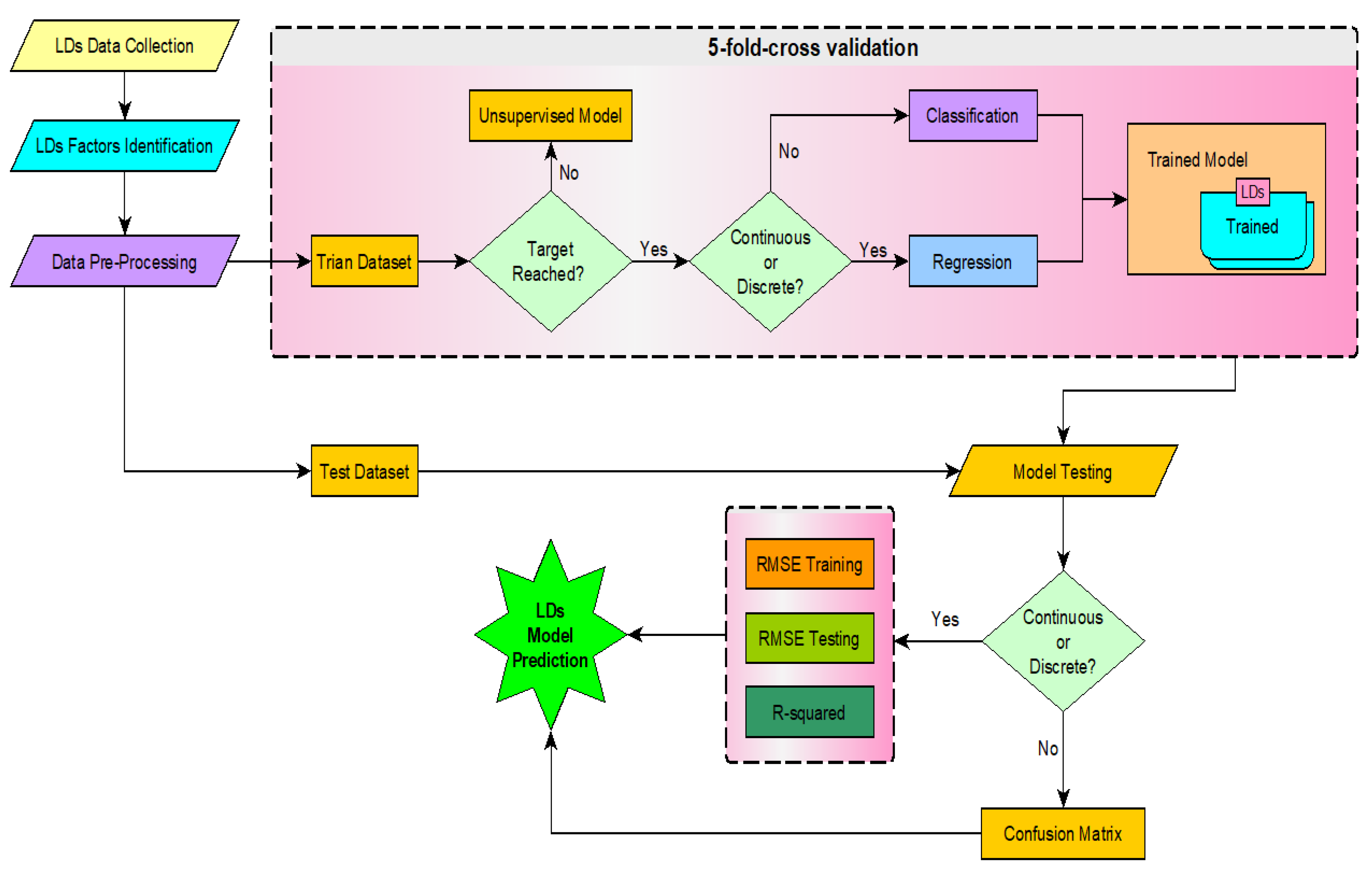
Development of the adopted linear regression algorithm was divided into the following major phases: (1) collection of related data from the Departments of Transportation (DOT), (2) defining all the factors affecting the LD, (3) sorting and processing the data to be more suitable for use in the stages of testing and training, (4) applying the concept of model development, and (5) evaluating the model performance with a model validation process. The linear regression model is illustrated in Figure 1 (where these five phases are shown) and will be discussed in the following sections. Finally, the model was validated using a 5-fold technique applied to train and test the developed model.

The decision-maker offers the proposed model to judge these disputes objectively. It provides the decision-maker with an insight into all the details and factors embedded in a conflict. Unfortunately, the authors have found no practical master tool for LD prediction in the literature, even though this conflict is a key issue in completing highway projects. Highway project contractors try to reduce their losses due to late project delivery by holding the owner accountable as the main reason behind late deliveries.

Delays can burden the contractor [22] with anticipated revenue being reduced. Contractors might even go bankrupt if they are unfamiliar with the potential additional costs incurred by LDs. Based on the contract, the highway project period is a key parameter to finishing the project at an appointed time. This model has been designed to help decision-makers deal with LD issues that can significantly delay project progress.

4. Data Collection Procedures and Preprocessing

4.1. Data Collection

We collected data from 2486 different road projects, with the six aforementioned factors from the DOT during the 6-year study period, to create a model with the flexibility to work with a wide variety of road construction projects that might appear in the future. Furthermore, the proposed model could be updated to handle additional road types that might need to be considered. Such data was recorded and exported into MS Excel sheets to prepare them for the analysis process. A comprehensive data source is essential for deep insight into the LD issues that can lead to conflict for all road project stakeholders. Therefore, data were collected for several major road systems (i.e., interstate, federal highway, state highway, county highway, rural roads, village roads, and district roads). Important factors included Bid Days, Total Bid Amount, Auto Liquidated Damage Indicator, Funding Indicator, and Total Adjustment Days, which play a key role in estimating the LD of road projects.

The data collection process collected the estimated LD amounts for road system projects as an independent variable. The DOT is a useful source for the variable labels, their associated data, and the details of the road projects. The obtained data allowed us to gain insight into the major factors in road projects. These factors were initially extracted from different DOT datasets and then manually exported to MS Excel sheets. Prognosticator features such as Bid Days, Road System Type, Total Bid Amount, Auto Liquidated Damage Indicator, Funding Indicator, and Total Adjustment Days were considered. The data were collected between 2012 and 2018. However, data conversion took about two years to guarantee that the collected data were adequate and useful for the Multiple Linear Regression (MLR) technique. A smart Excel script was designed to collect all factors that play a part in creating the MLR models. The data were distributed into six factors, as shown in

Table 1. Variable descriptions for Liquidated Damage estimation for the road systems.

Variable Label	Variable Identification	Type of Variable	Description
Bid Days	X1	Numerical	The original number of days for the contract.
Road System Type	X2	Categorical	The type of road system: Interstate Federal highway State highway County highway Rural roads or village roads, and District roads
Total Bid Amount	X3	Numerical	The amount of the bid of the contract awarded to the job.
Auto Liquidated Damage Indicator	X4	Categorical	Indicates whether liquidated damages will be calculated or not. Must be 1. ‘N’ (No) or 2. ‘Y’ (Yes)
Funding Indicator	X5	Categorical	Indicates how the contract is funded (i.e., 1. B—both federal and nonfederal funds, or 2. F—federal funds only)
Total Adjustment Days	X6	Numerical	Total charge days for a contract. Derived field—summation of adjusted days contract change order table.

. Most of the data was saved as a numerical value, representing the variables used in the linear regression model.

4.2. Features Engineering

Six features of road system data were used as independent variables for highway construction projects to generate MLR models for estimating LDs. The factors used in the proposed model can be classified into two categories (i.e., Numerical and Categorical). Variables, along with their descriptions, are itemized in Table 1.

4.3. Data Preprocessing

Data preprocessing is key to the employment of $\mathrm{multiple} \mathrm{linear} \mathrm{regression}$ algorithms. Variable selection chooses variables that will be significant for $\mathrm{LD}$ prediction. Preprocessing involves outlier cleaning, removal of data noise, normalization, standardization, characteristic assortment, and conversion. The data collected included both categorical and numerical values for the selected variables.

Once the appropriate variables are selected, preprocessing is required, including outlier elimination and dataset normalization. This first step of data preprocessing eliminates outliers from the collected data. Without eliminating these outliers, many variabilities and mistakes will reduce the efficiency of the linear regression technique. Interquartile ranges were employed to reveal extreme and outlier values in this work. Appropriate graphical approaches, such as Boxplots for outlier removal, have also been employed. Null indicators were also employed to represent and eliminate missing values from the data collected.

Reliability issues can appear when data points are missing from the original database. The missing data might be related to any factor (such as Bid Days or Road System Type). Therefore, missing values within the dataset (i.e., values which are represented with either the “Null” or “-” indicators) were considered. A small percentage of missing data (i.e., 114 missing values representing about 4.6% of the original database) required preprocessing. These missing data points were replaced using those attributes’ average and median values.

The transformation process is the second phase of preprocessing. The dataset contained three numerical and three categorical features. The numerical features list included: (1) Bid Days, (2) Total Bid Amount, and (3) Total Adjustment Days. The categorical features list included: (1) Road System Type, (2) Auto Liquidated Damage Indicator, and (3) Funding Indicator. Categorical variable values were converted into integers to guarantee convergence and a smooth modeling system. In doing so, the whole database was transformed to include only numerical values for all the variables. A suitable approach was employed to ensure an appropriate conversion process, called a characteristic assortment.

5. Multiple Linear Regression Model Development

Multiple Linear Regression (MLR) is employed for numerical predictions and is generally used to model linear behavior [23]. The variables in the dataset are labeled as independent and dependent variables. This technique is widely used for numerical value forecasting based on linear regression parameters. The MLR approach is suitable for discovering relationships between a dependent variable and a set of independent variables. A least-squares approach is used to estimate the values of the model’s coefficients. Various model assumptions were assessed in our work, and adjustments were made before selecting a suitable model. (Details about the evaluations of these various models will be discussed later.) An $\mathrm{MLR}$ model based on several independent variables, $X_1, X_2, X_3,\dots \dots X_n$, which meets the assumptions of a linear regression model can be expressed by the Equation (1)

$$Y={\beta }_0+{\beta }_1{X}_1+{\beta }_2 \left(X_2\right)+{\beta }_3 \left(X_3\right)+\cdots +{\beta }_n{X}_n+\epsilon$$

(1)

where $Y$ is the response variable, $X_1, X_2, X_3\dots X_n$ are the predictor variables, ${\beta }_n$ are the collection of regression coefficients, and $\mathsf{\epsilon }$ is an error value, where Figure 2 illustrates Equation (1):

Our regression model is stated in Equation (2).

$$\widehat{Y}={\widehat{\beta }}_0+{\widehat{\beta }}_1{X}_1+{\widehat{\beta }}_2{X}_2+\cdots +{\widehat{\beta }}_K{X}_K$$

(2)

where $\widehat{Y}$ represents the predicted value and ${\widehat{\beta }}_K$ represents an estimate of the collection of regression coefficients.

Equation (3) calculates the summation of the deviation’s squares (residuals) of the obtained value of $Y$ formula. The equation with the minimum value of the $SS\left(residual\right)$ is the “best fit” equation for the given dataset.

$$\begin{array}{cc}SS\left(residual\right)\hfill & ={\displaystyle \sum }_{i=1}^n{\left[Y_i-{\widehat{Y}}_i\right]}^2\hfill \\ & ={\displaystyle \sum }_{i=1}^n{\left[Y_i-{\widehat{\beta }}_0+{\widehat{\beta }}_1{X}_1+{\widehat{\beta }}_2{X}_2+\dots +{\widehat{\beta }}_K{X}_{Ki}\right]}^2 \hfill \end{array}$$

(3)

where $Y={\beta }_0+{\beta }_1{X}_1+{\beta }_2{X}_2+\dots +{\beta }_k{X}_K$ represents the predicted value produced by the proposed model, and ${\beta }_k$ represents an estimate of the coefficients needed to provide a good estimate with the proposed model.

5.1. Multiple and Stepwise Linear Regression

Multiple linear regression (MLR) can be applied to predict the value of a dependent variable, $Y_i$, based on the values of a set of independent variables, $x_{ij}$. $\mathrm{As} \mathrm{mentioned} \mathrm{earlier},$ the MLR model can be defined using Equation (4).

$$Y_i={\displaystyle \sum }_{j=1}^k{B}_j{x}_{ij}+{\epsilon }_i$$

(4)

where $k$ represents the number of the independent variables, $B_j$ represents the k coefficients of the linear regression, $x_{ij}$ represents the $j$ values for the observation $i$, and ${\epsilon }_i$ represents the residual error.

5.2. Statistical Hypothesis

Hypotheses were developed for this study. First, the null hypothesis states no correlation between the dependent variable LD and the six independent variables of Bid Days, Road System Type, Total Bid Amount, Auto Liquidated Damage Indicator, Funding Indicator, and Total Adjustment Days, as shown in Equation (5).

Testing Significance of Regression:

$${\beta }_1={\beta }_2={\beta }_3={\beta }_4={\beta }_5={\beta }_6=0$$

(5)

The p-value is a number calculated from a statistical test. It describes how likely you are to have found a particular set of observations if the null hypothesis were true. p-value are used in hypothesis testing to help decide whether to reject the null hypothesis. The smaller the p-value, the more likely you are to reject the null hypothesis. If the p-value for any of these six correlation coefficients is less than $0.05$, the correlation is defined as significant. If the p-value for these correlation coefficients is less than $0.01$, then the correlation is defined as highly significant.

5.3. Criteria for Employing Mulitple Linear Progression

Not all datasets can be well modeled with Multiple Linear Regression. Therefore, when MLR is applied to a dataset, the following criteria can be applied to the predictions to determine whether that dataset is suitable for modeling with MLR:

• Residuals: When errors between observed and predicted values are plotted against the values of each independent variable, there should be no predictable patterns or trends. A horizontal line (with only random peaks or dips) indicates a linear relationship between that independent variable and the prediction.
• Normality: Errors between observed and predicted values should form a normal distribution. The degree of normality can be visualized using a Q-Q-Plot, which plots the histogram of a normal distribution against the MLR model’s predictions. A straight line results when the histogram of a normal distribution is plotted against the histogram of another normal distribution. Conversely, when the histogram of a normal distribution is plotted against the histogram of a less-then-normal distribution, the crookedness of the line indicates the degree to which the latter departs from a normal distribution.
• Scale-Location (heteroscedastic): The variance of the errors should not be constant across observations. Heteroscedastic is the condition in which the residual period in a regression model varies.
• Residuals vs. Leverage is used to find the values of independent variables that greatly affect the regression results, as seen when they are included or excluded from the training set.
• Multicollinearity: When independent variables are correlated, multicollinearity is present. If two independent variables are perfectly correlated, no unique set of coefficients provides an optimal solution, and the training process might not converge.

6. Modeling Training and Testing

The evaluation of the model involves examining (1) the “goodness of fit” between the values of the dependent variable (as contained in the dataset) and the corresponding values predicted by the model, (2) whether the residuals are random, and (3) whether the model’s performance deteriorates significantly when applied to data that were not used when training the model.

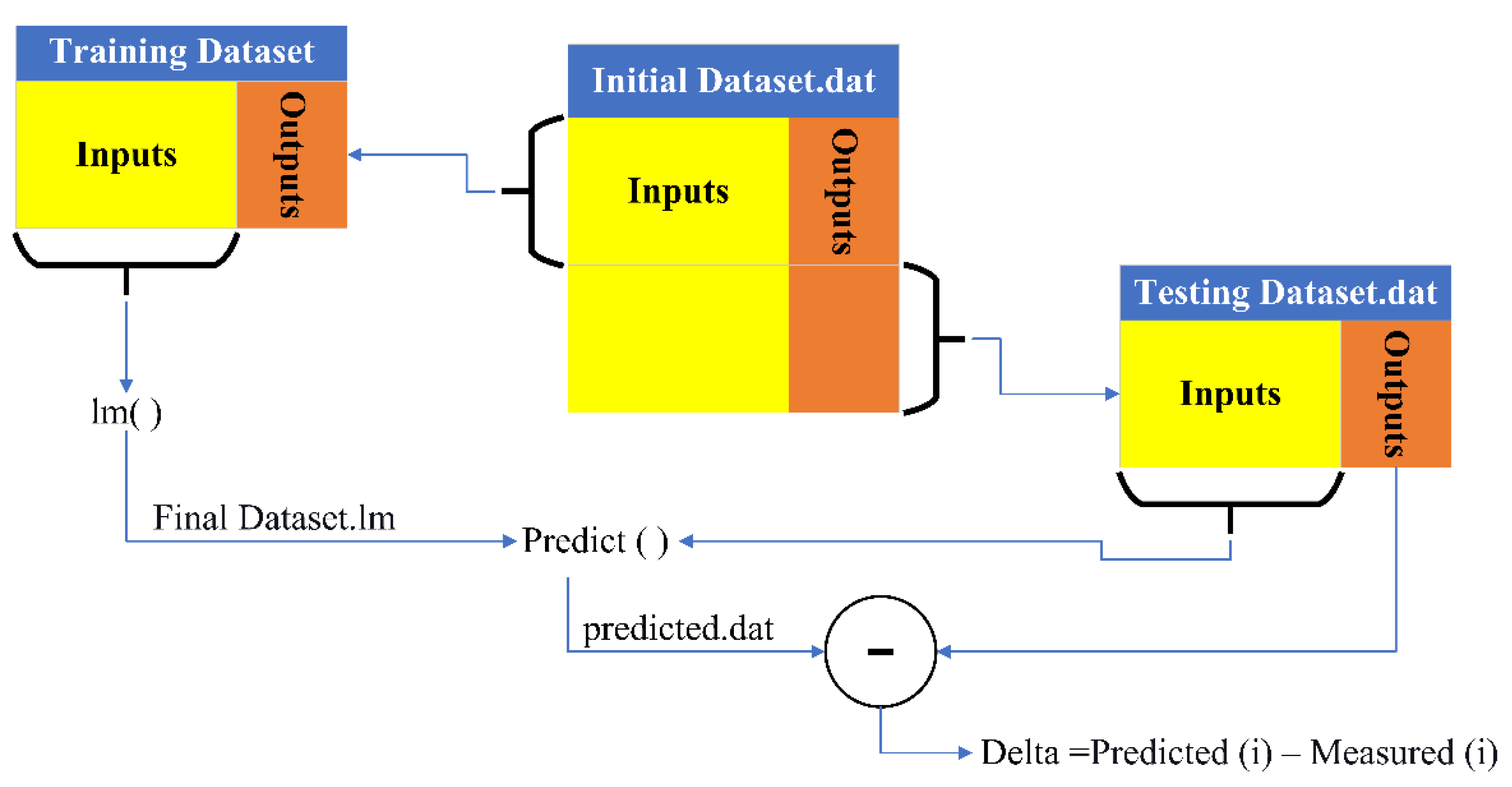
The latter (3) was accomplished by dividing the dataset into a training subset (70%, 1659 samples) and a testing subset (30%, 711 samples). The training dataset was then used to train the model, and the testing dataset was used to evaluate the model. This training and testing dataset process are illustrated in Figure 3.

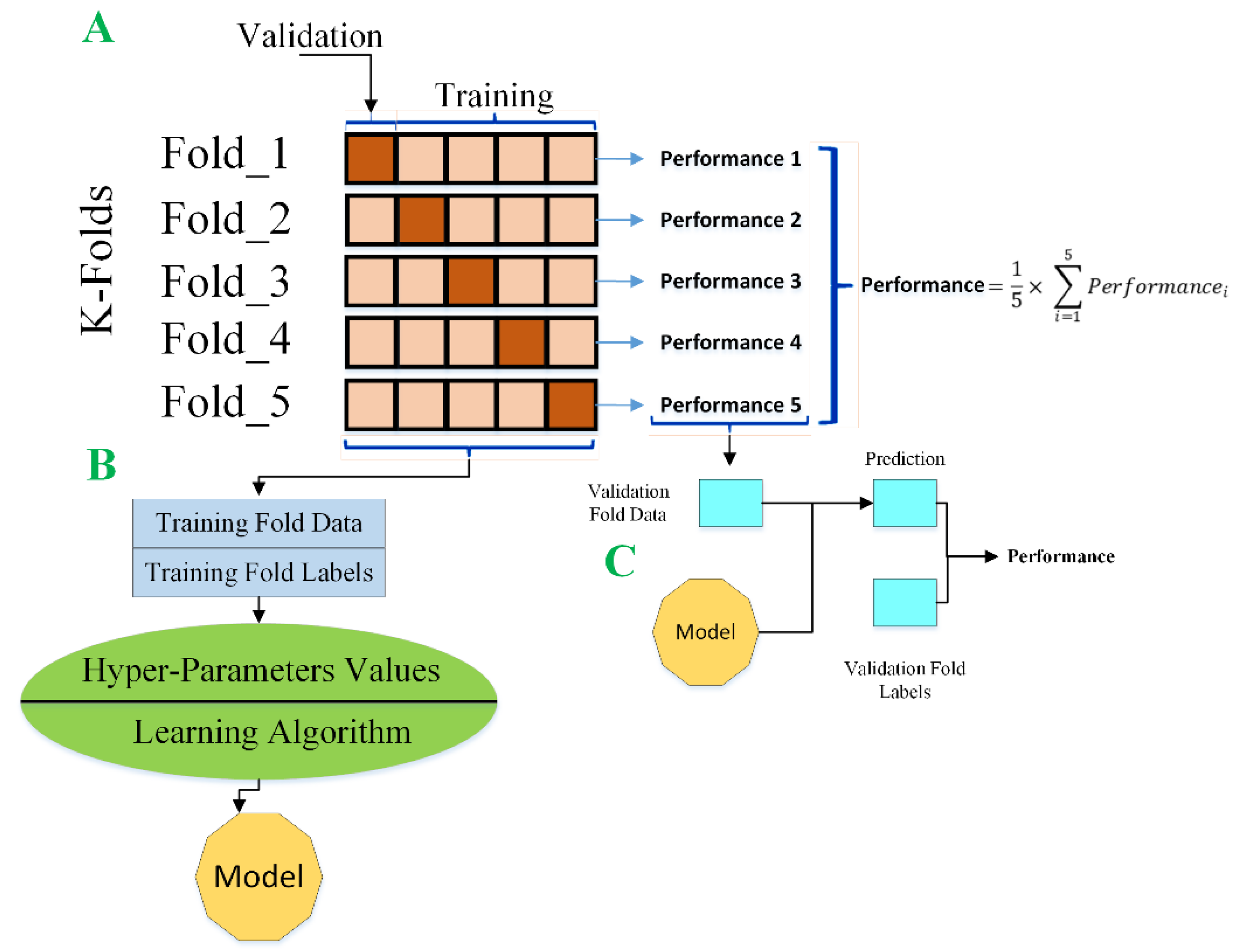
Model Validation (K-Fold Cross-Validation)

A method called K-Fold cross-validation is used to evaluate the robustness of a linear regression model [24]. First, the data in the database is subdivided into K subsets. Then, k-1 of these subsets is used as the training set, while the remaining subset is used as the testing set to measure performance, as shown in Figure 4. This process is repeated until every subset has been used as the testing set.

7. Evaluating the Performance of MLR

After validating the criteria for employing MLR and evaluating the MLR model with K-Fold cross-validation, it is appropriate to measure the model’s predictive capacity using various metrics. Our work has employed Root Mean Squared Error (RMSE), Trained Root Mean Squared Error ($RMS{E}_{Train}$), Tested Root Mean Squared Error ($RMS{E}_{Test}$), and R-Squared ($R^2) metrics$ to evaluate the model.

The Root Mean Squared Error $\left(RMSE\right)$ calculates the accuracy of linear regression models in terms of their error, as shown in Equation (6). The accuracy is higher if this error value is closer to zero.

$$RMSE\left(\widehat{f}, Data set\right)=\sqrt{\frac{1}{n}{\displaystyle \sum }_{i=1}^n{\left(y_i-{\widehat{f}}_{\left(xi\right)}\right)}^2}$$

(6)

where $n$ is the number of cases that are applied to the linear model,${\widehat{f}}_{\left(xi\right)}$ is the predicted value for the i-th case, and $y_i$ is the actual value for the i-th case. Ideally, ${\widehat{y}}_{\left(xi\right)}={\widehat{f}}_{\left(xi\right)}$.

8. Applying the RMSE Metric to Our MLR Model

The train $\left(RMSE\right)$ and test $\left(RMSE\right)$ are represented in Equations (7) and (8), respectively, where $n_{Train}$ and $n_{Test}$ represent the number of data elements in the training and testing sets, respectively.

$$\begin{array}{cc}{\mathit{RMSE}}_{Train}=\hfill & RMSE\left(\widehat{f}, Train Data set\right)\hfill \\ & =\sqrt{\frac{1}{n_{Train}}{\displaystyle \sum }_{i\in Train}{\left(y_i-{\widehat{f}}_{\left(xi\right)}\right)}^2}\hfill \end{array}$$

(7)

$$\begin{array}{cc}{\mathit{RMSE}}_{Test}=\hfill & RMSE\left(\widehat{f}, Test Data set\right)\hfill \\ & =\sqrt{\frac{1}{n_{Test}}{\displaystyle \sum }_{i\in Test}{\left(y_i-{\widehat{f}}_{\left(xi\right)}\right)}^2}\hfill \end{array}$$

(8)

Another widely used method has been applied to measure the best fit for the straight line of the proposed model, which is called R-Squared ($R^2$); this value is calculated as shown in Equation (9).

$$R^2=1-\frac{SS\left(Residual\right)}{SS\left(Total\right)}$$

(9)

where the $SS\left(Total\right)$ is the summation of the squared differences from the average value of the dependent variable values. In other words, $R^2$ compares the variance around the average line to the variation around the linear regression line.

Adjusted $R^2$ is also a useful method applied in this model, as shown in Equation (10).

$$R_{Adjusted}^2=1-\left[\frac{SS\left(Residual\right)}{SS\left(Total\right)}\right]\times \left[\frac{\left(n-1\right)}{\left(n-d-1\right)}\right]$$

(10)

where $n$ represents the number of sample data elements for the training dataset, and $d$ represents the polynomial degree of the proposed model. The values of $R^2$ and $R_{Adjusted}^2$ are computed to decide if the additional terms of $n$ and $d$ enhance the predictive power of the proposed model.

9. Results and Discussion

Descriptive Statistics of the Dataset and Visualizing the Relationships in the Data

In the dataset provided, there were six independent (predictor) variables and one dependent (response) variable: The independent variables were Bid Days, Road System Type, Total Bid Amount, Auto Liquidated Damage Indicator, Funding Indicator, and Total Adjustment Days, and the one dependent variable was the LD prediction.

Before a regression model is selected, it is sensible to look at a scatterplot matrix of the independent variables (predictors) and the dependent variable (all taken from the dataset) to gauge whether linear regression is appropriate and, if so, what model should be chosen. A scatterplot matrix is a grid of scatterplots where each of the variables in the dataset is plotted against the other variables in the dataset. It visualizes the relationships between pairs of variables.

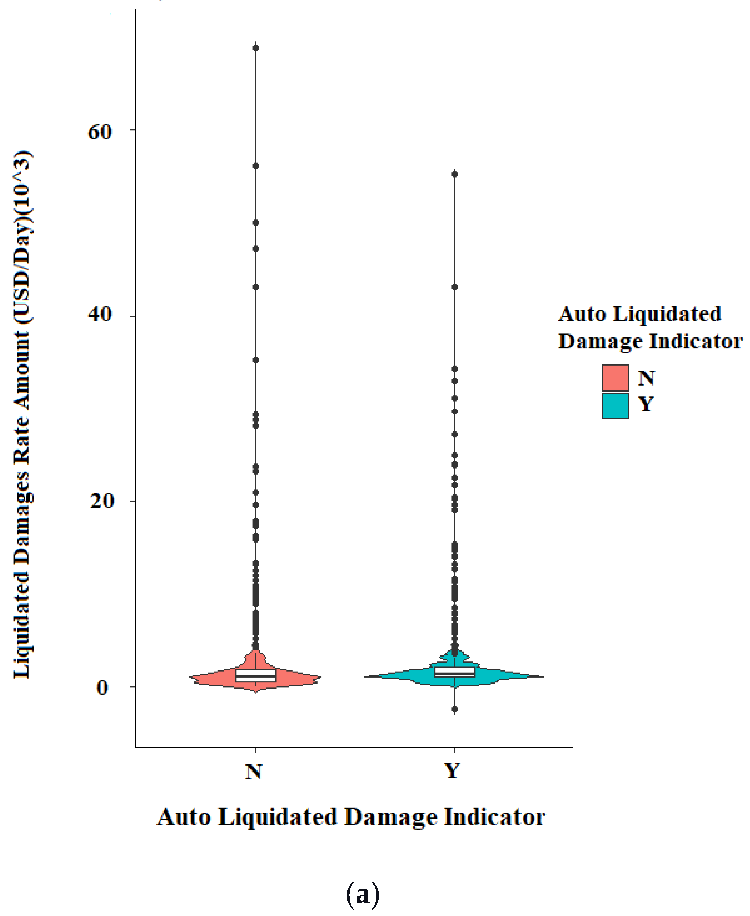
The three categorical independent variables (Auto Liquidated Damage Indicator, Funding Indicator, and Road Systems) were plotted against their corresponding Liquidated Damages (LDs) in the database, as shown in Figure 5a–c. These three scatterplot matrices show some correlation between Road System Type and LDs, but not much correlation for Auto Liquidated Damage Indicator or Funding Indicator. In addition, all three scatterplots indicate the presence of many outliers.

As shown in Figure 6a–c, the three numerical independent variables (Bid Days, Total Bid Amount, and Total Adjustment Days) have a strongly skewed distribution. The graph looks like a log-normal distribution, which can be defined as a distribution whose logarithm is normally distributed. It is essential to transform variables into a normal distribution to handle this problem.

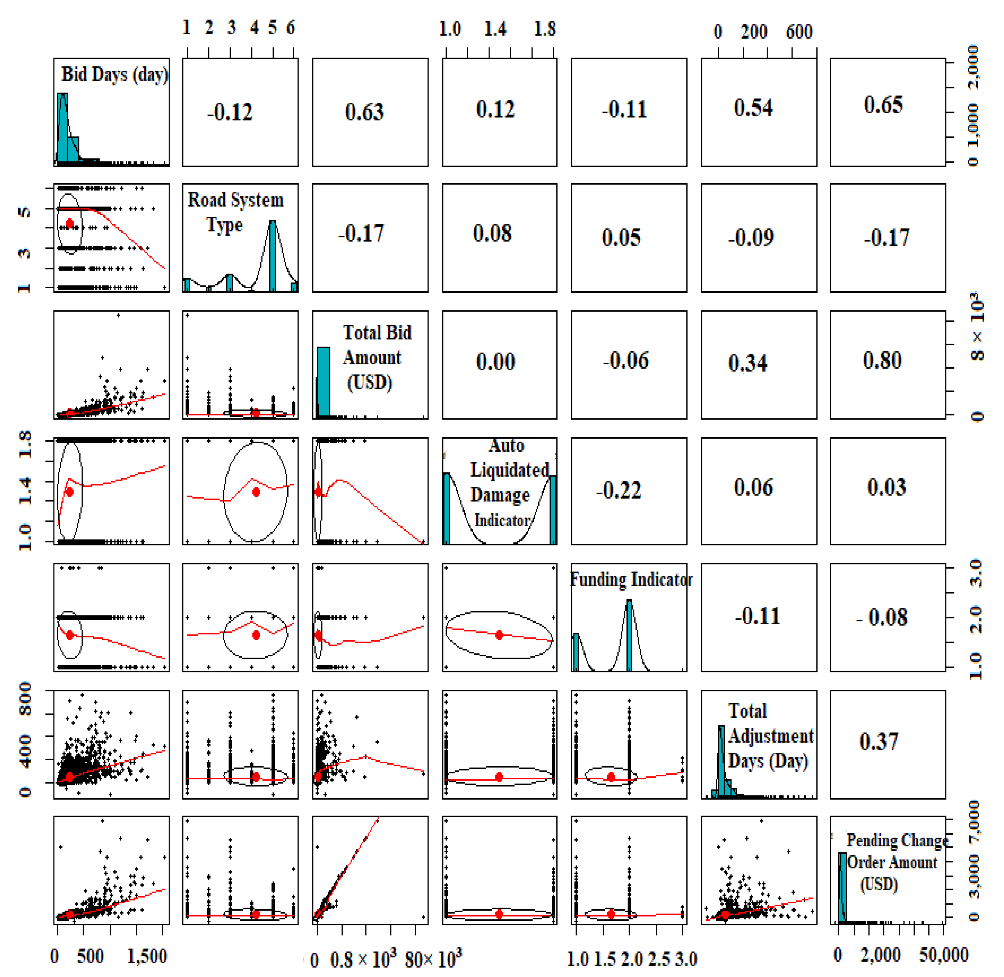
Figure 7 shows the scatterplot matrix for the entire dataset. It shows a robust correlation between only a few of the independent variables.

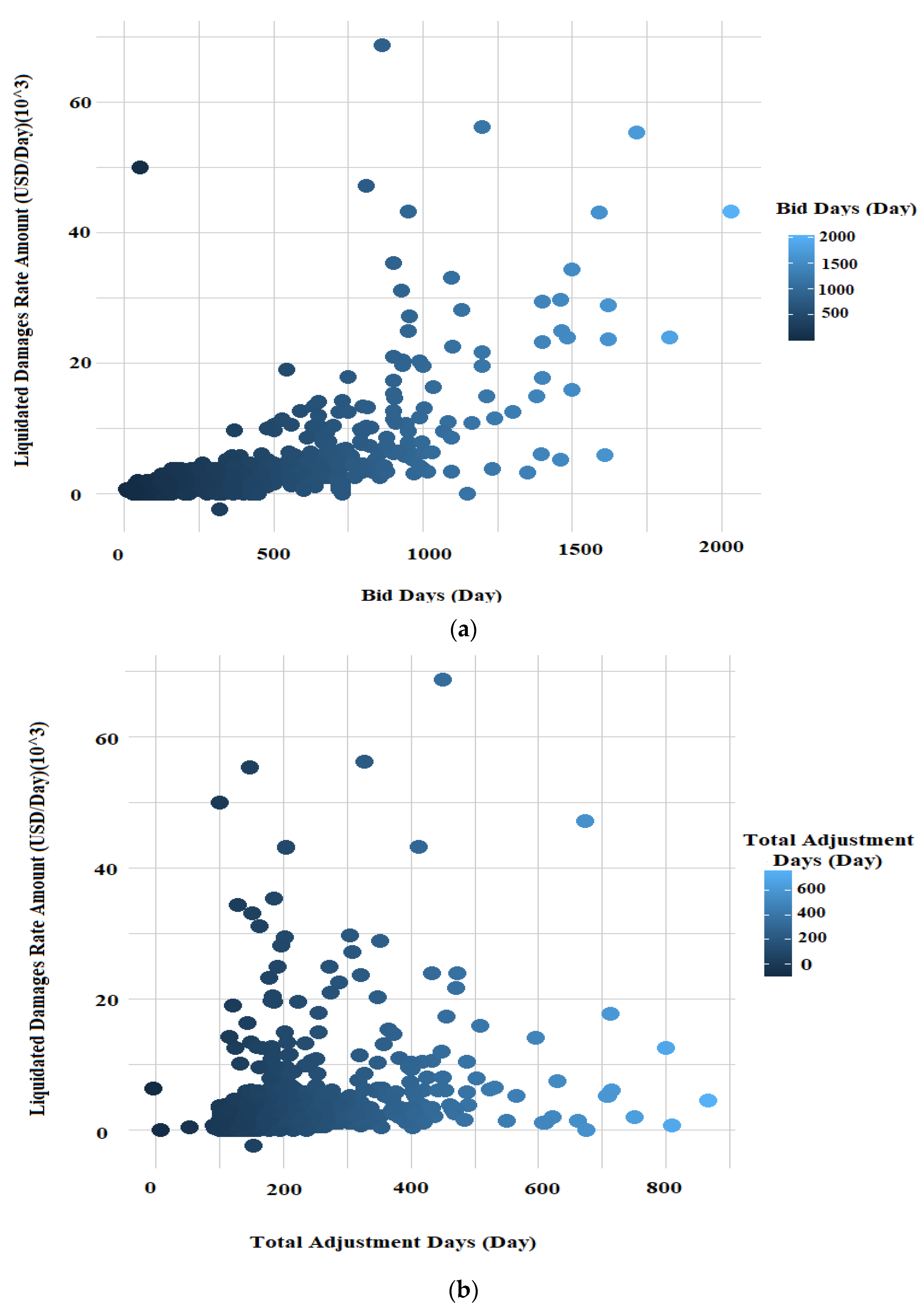
Figure 8 shows a scatterplot matrix for the three numerical independent variables: Bid Days, Total Adjustment Days, and Total Bid Amount. These scatterplots show a clear increase in Liquidated Damages (LDs) as Bid Days, Total Adjustment Days, and Total Bid Amount increase. There is an obvious linear correlation between Total Bid Amounts and LDs. However, the correlations between LDs and Bid Days and LDs and Total Adjustment Days are less clear. These nonlinear relationships would need to be modeled. Polynomial terms might not be flexible enough to capture these complex relationships. Overall, it is unclear how well the MLR prediction mechanism will perform on this dataset in an integrated manner.

As mentioned earlier, not all datasets can be well modeled with Multiple Linear Regression. Therefore, to determine whether our dataset is suitable for modeling with MLR, we applied the following criteria to the predictions of our model:

1.

Normal Q-Q:

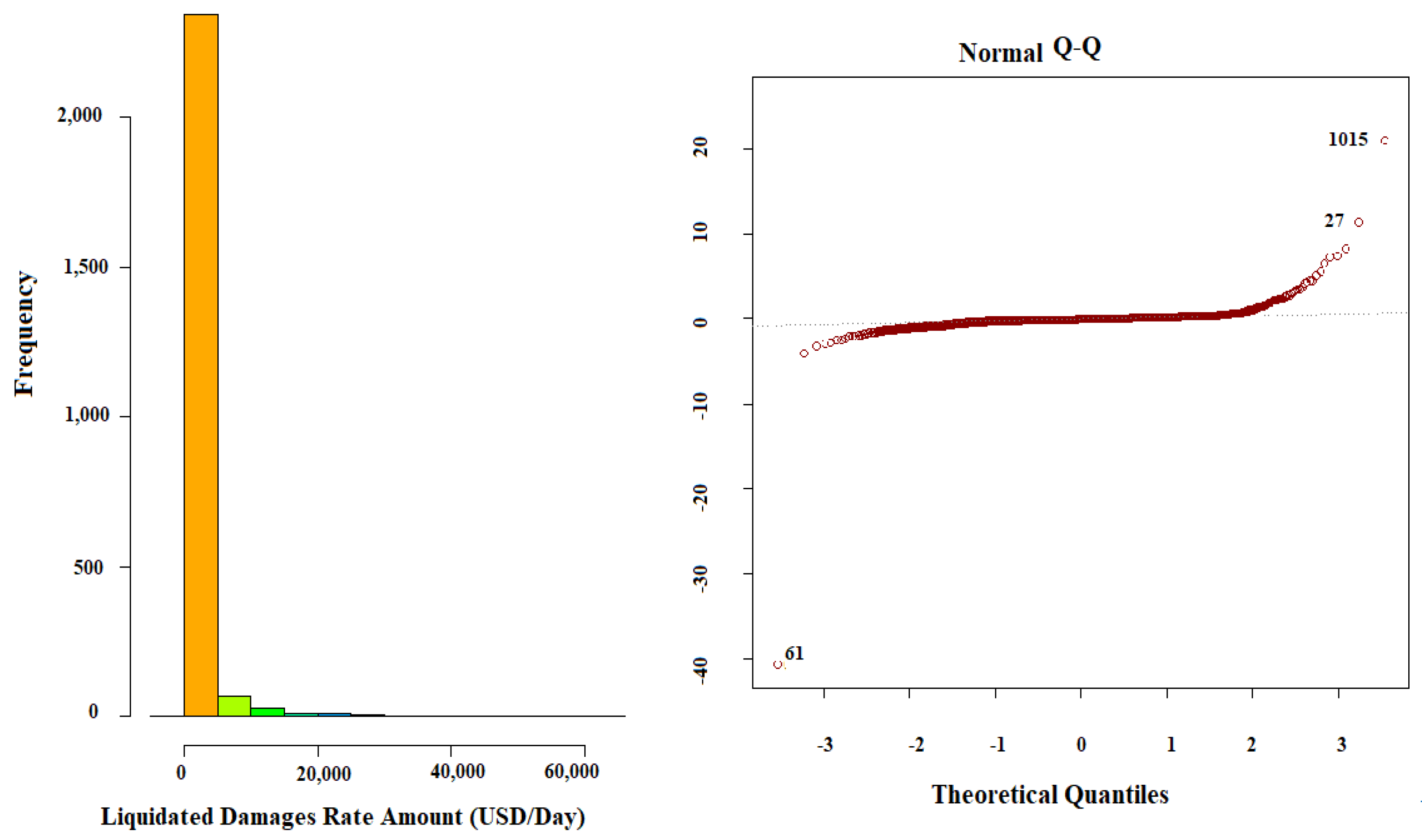
Errors between observed and predicted values should form a normal distribution. The degree of normality can be visualized using a Q-Q-Plot, which plots the histogram of a normal distribution against the MLR model’s predictions. If this produces a straight line, the residuals have a normal distribution. Based on the strongly skewed distributions of the dependent variable in Figure 9, it was expected that the MLR model trained from that data would not have a normal distribution. As expected, the Q-Q-Plot did not show that the residuals from the model were normally distributed. To obtain a normal distribution, the data would need to be transformed.

2.

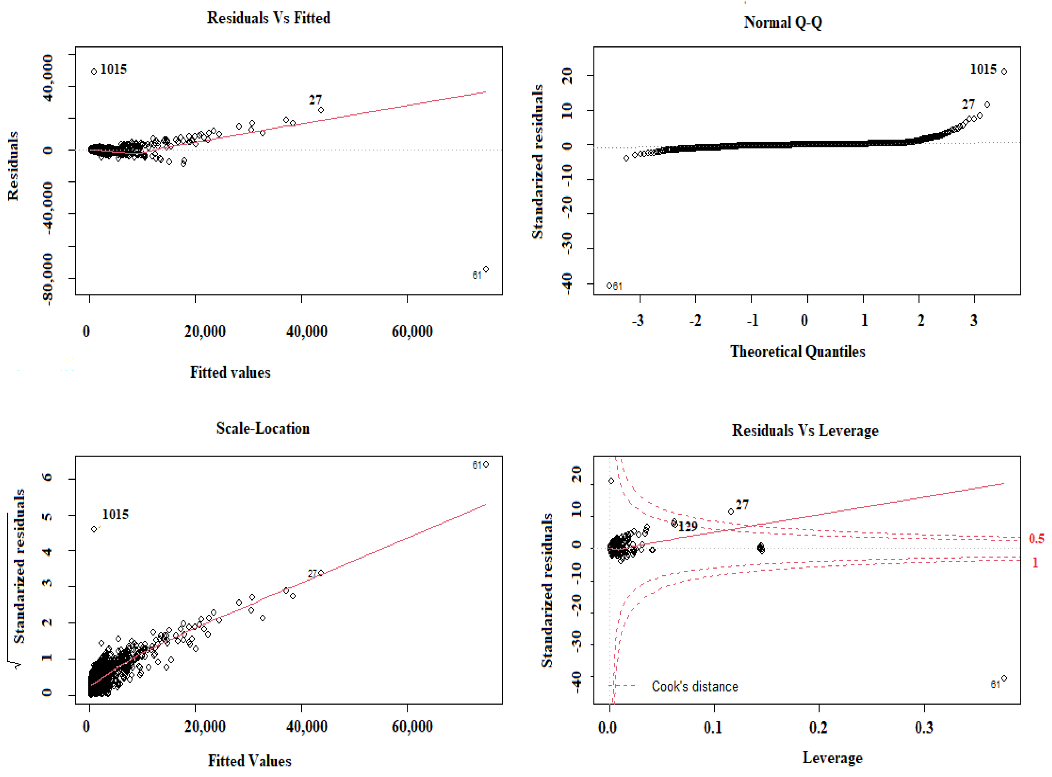
Residuals vs. Fitted Plot:

When errors between observed and predicted values are plotted against the values of each independent variable, there should be no predictable patterns or trends. A horizontal line (with only random peaks or dips) indicates a linear relationship between that independent variable and the prediction. The residuals vs. fitted plot below shows that the MLR model’s residuals grow in spread from left to right and seem to follow a downtrend. This means that the model still suffers from heteroscedasticity; running a Breusch–Pagan test and a Goldfeld–Quandt test on the model yields the following results [25].

3.

Scale-Location Plot (Spread-Location):

The variance of the errors should not be constant across observations. Heteroscedastic is the condition in which the residual period in a regression model varies. This graph displays how the residuals are spread and checks the residuals’ homogeneity of variance (homoscedasticity) when residuals are randomly spread near a horizontal line. This graph increases the red line from left to right because the residuals’ increase from left to right.

4.

Residuals vs. Leverage Plot:

Residuals vs. Leverage is used to find values of independent variables that greatly affect the regression results, as seen when they are included or excluded from the training set. The Cook’s distance of a point measures how influential the point is in determining the model’s coefficients. It can be seen from the scale-location plot that there is a movement in the following trend, which is difficult to see on the residuals vs. fitted plot partly because some points have very large residuals, which means that the model suffers from heteroscedasticity. Running a “bptest” on the model is vital to ensure that the observation is correct. There are three points of high Leverage but no influential points. Such a point is not influential, since it falls out of the acceptable boundary between the lower and upper dashed lines, which may be taken out of the dataset to attain a model free of the influence of such a point, as shown in Figure 10, which is vital to identify the influential points considered within the analysis.

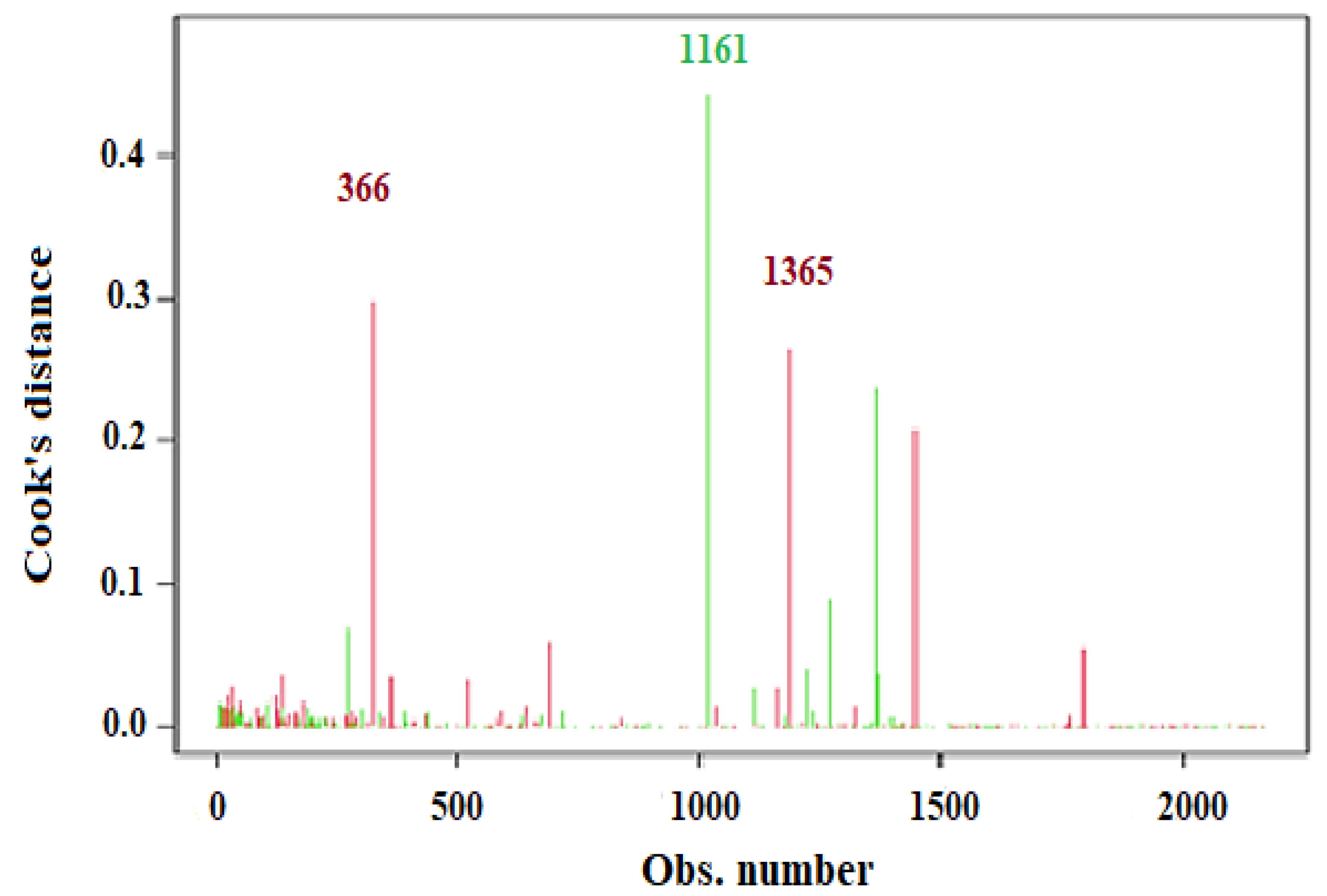
Cook’s distance was examined to check for influential data points using Influential Observations, since they have an unequal impact on the model coefficient values. Figure 11 provides a plot of Cook’s distances by observation, which flags observations 366, 1161, and 1365 as particularly influential. Dropping these observations may have a notable impact on improving the model and the intercept and slope values.

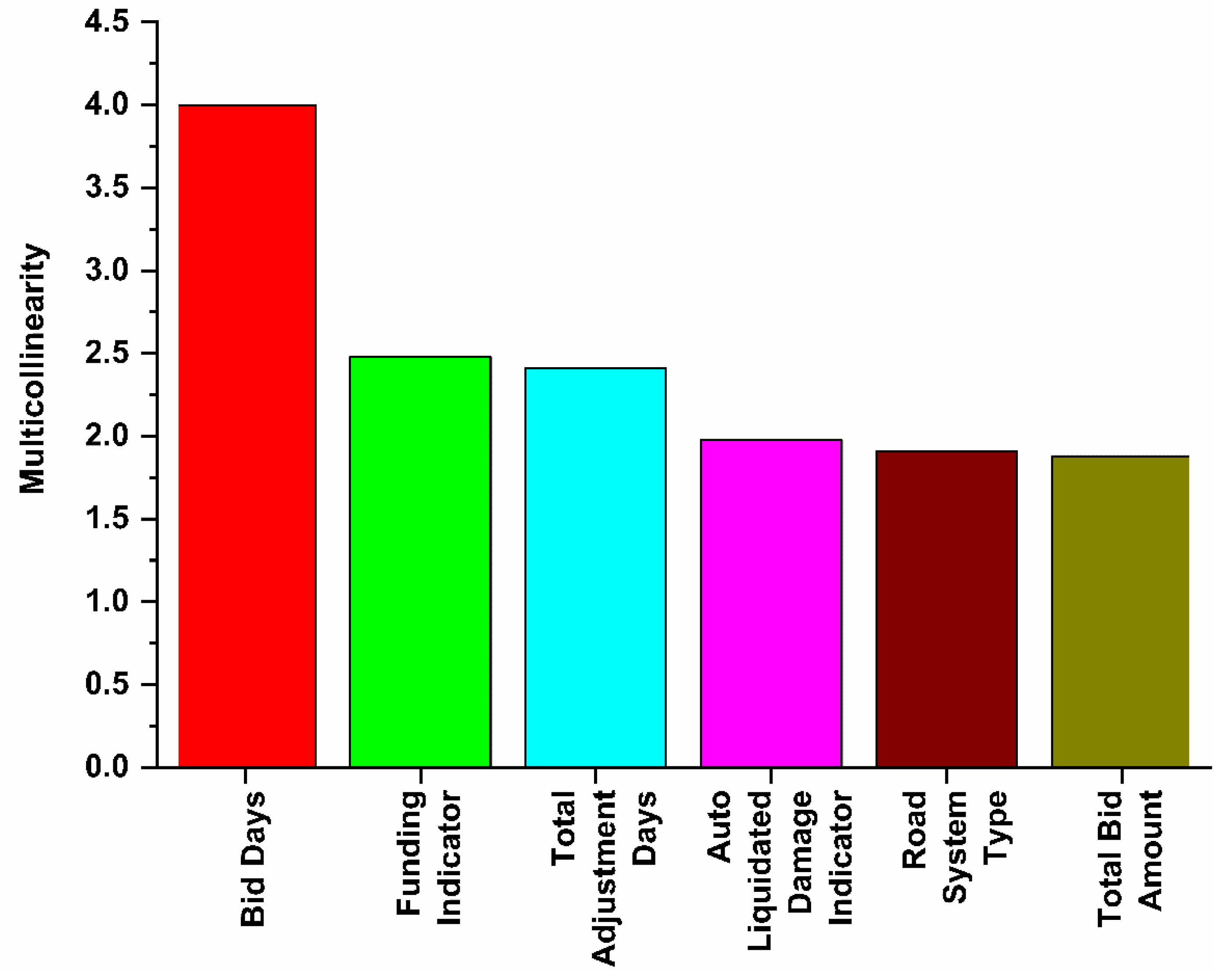
Multicollinearity was the first assumption tested between the independent variables. Some independent (predictor) variables are correlated with others. Several procedures have been developed to identify extremely collinear predictor variables and for likely resolutions to the problem of multicollinearity. The presence of serious multicollinearity often does not affect the usefulness of the fitted model for estimating mean responses or making predictions. The values of the predictor variables for which inferences are to be made follow the same multicollinearity pattern as the data on which the regression model is based. Hence, one remedial measure is to restrict the use of the fitted regression model to inferences for values of the predictor variables that follow the same pattern of multicollinearity. Multicollinearity was applied using the Variance Inflation Factor (VIF). The results show no multicollinearity, since a VIF less than 10 shows a high value of VIF, as shown in Figure 12.

10. Modified MLR Prediction Model Fitting and Assumptions

Given the problems listed above, an ordinary MLR prediction model was not satisfactory. Figure 13 shows a step-by-step approach to constructing a modified MLR model. Many of these steps were applied in this study to derive a modified MLR model suitable for the aimed goals.

Subsequently, regression checking was performed on this modified MLR model to determine whether there was multicollinearity. If the $VIF>10$, it is necessary to remove the variable with high multicollinearity.

Six variables were ultimately selected to build a full model. A linear equation might be satisfactory, but a second-order term can be combined to take care of curving.

A regression analysis was performed on the modified MLR model with the software package. At least one of the regression coefficients is different from zero. The simplest model used forward entry, backward removal, forward stepwise, backward stepwise, and best-subset search procedures.

To train the MLR model, finding the model that better explains the data variability is necessary. Therefore, the dataset was divided into a training subset (70%) and a testing subset (30%). Seven modified models were applied and compared, as shown in

Table 2. Train $RMSE$, Test $RMSE$, and Prediction analysis results.

Modified Models	Train $RMSE$	Test $RMSE$	Prediction
$\mathit{F}\mathbf{i}\mathbf{t}\mathbf{\_}\mathbf{1}$	848.528	1173.050	6
$\mathit{F}\mathit{i}\mathit{t}\mathbf{\_}\mathbf{2}$	841.861	1138.042	8
$\mathit{F}\mathit{i}\mathit{t}\mathbf{\_}\mathbf{3}$	832.811	1126.947	16
$\mathit{F}\mathit{i}\mathit{t}\mathbf{\_}\mathbf{4}$	829.037	1118.239	17
$\mathit{F}\mathit{i}\mathit{t}\mathbf{\_}\mathbf{5}$	796.302	1212.407	32
$\mathit{F}\mathit{i}\mathit{t}\mathbf{\_}\mathbf{6}$	736.499	1323.668	63
$\mathit{F}\mathit{i}\mathit{t}\mathbf{\_}\mathbf{7}$	736.791	1333.791	64

.

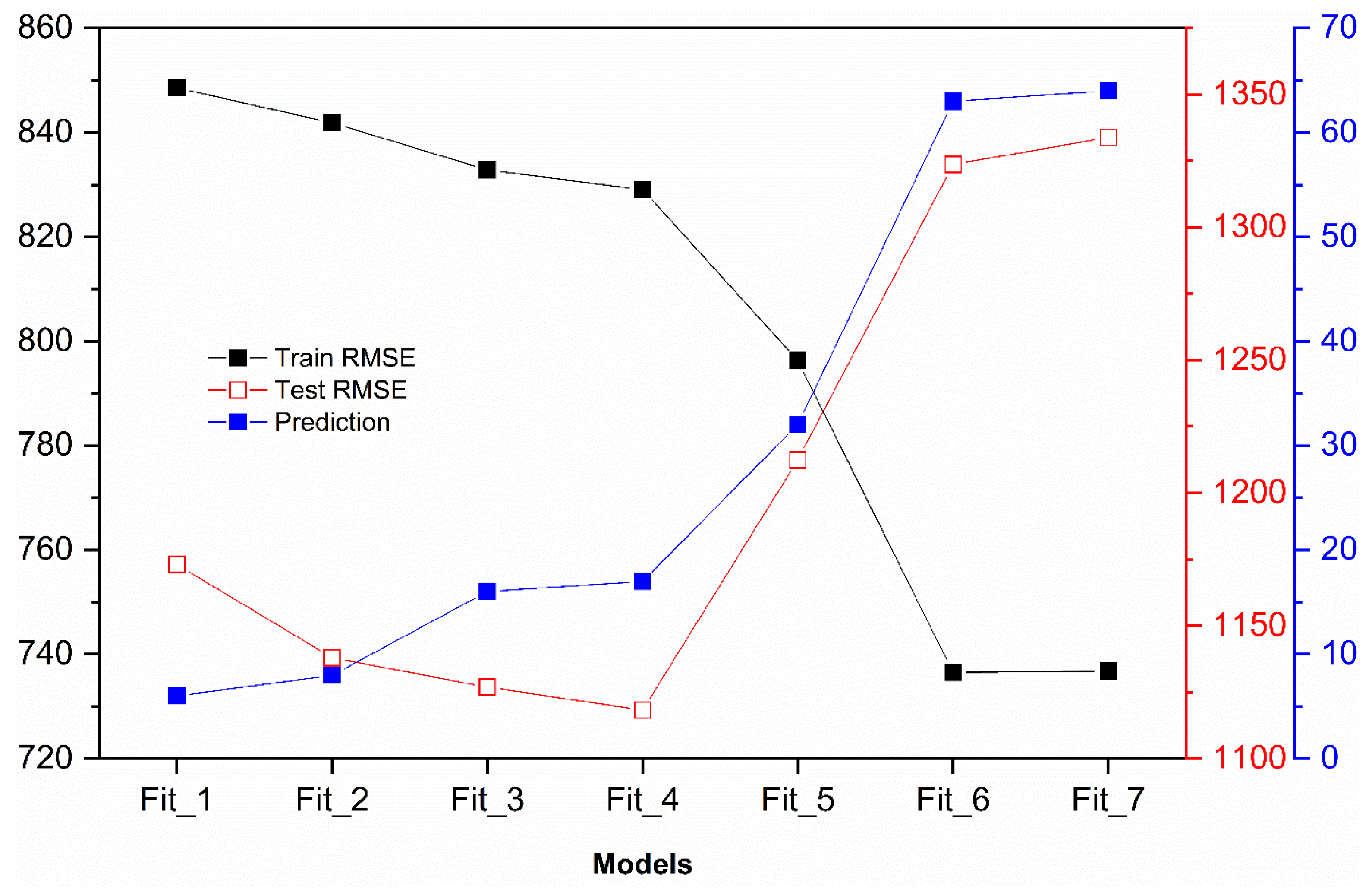
Figure 14 summarizes the results for the best-fit model. $Fit\_1$ is the least flexible, and $Fit\_6$ is the most flexible. Furthermore, the Train RMSE decreases as flexibility increases in $Fit\_1$, $Fit\_2$, and $Fit\_3$. These three models were described as underfitting models since they have a high Train $RMSE$ and a high Test $RMSE.$ (A model is underfitting if there exists a more complex model with lower Test $RMSE$.)

$Fit\_5$, $Fit\_6$, and $Fit\_7$ are overfitting models since they have low Train $RMSE$ and high Test $RMSE$. These models are overfitting since there exists a less complex model with a lower Test $RMSE$.

Any more complex model with higher Test $RMSE$ is overfitting. Any less complex model with higher Test $RMSE$ is underfitting. The Test $RMSE$ is the smallest for $Fit\_4,$ suggesting that it will perform best on future data not used to train the model.

Figure 14 compares the modified models in their Train $RMSE$, Test $RMSE$, and Prediction. The graph shows that the model $Fit\_4$ has the lowest Test $RMSE$. Hence, model 4 was judged to be the best. Its predictions met all the statistical criteria used to evaluate whether a model is suitable for our dataset. Moreover, no patterns were noticed in the residuals compared to the independent variables used in the model, demonstrating that no important variables were omitted.

The variable with the most significant residual, such that $P<t$, was removed. An assessment removed the three feathers since they seemed to not affect the model and were not significant for the model. Transformations were used since some feathers were nonlinear. The p-values indicate that the linear and squared terms are statistically significant in the statistical output below. From the Analysis of Variance table, the p-value was less than $0.05 \left(2.2 {10}^{-16}\right)$, which suggests that the best modified MLR model is significant at an $\alpha -level$ of $0.05$. Accordingly, this proposed modified MLR model is validated, and it is expected to provide a statistically significant and unbiased fit to these data.

However, additional issues must be considered before this model can be used to make predictions. Therefore, the modified MLR model was simplified by removing a limited number of datapoints. The following second-order model (See Equation (11)) with interaction was adopted based on the reasoning above.

$$y=8.08{\mathrm{e}}^2-7.17{\mathrm{e}}^{-1}B+2.54{\mathrm{e}}^2 \mathrm{R}-2.77{\mathrm{e}}^{-4}\mathrm{T}-9.80{\mathrm{e}}^{1}A-3.85{\mathrm{e}}^1{R}^2+6.62{\mathrm{e}}^{-4}{B}^2+\epsilon$$

(11)

where $B$ represents the Bid Days, $R$ represents Road System Type, $\mathrm{T}$ represents the Total Bid Amount, and $A$ is the Auto Liquidated Damage Indicator.

Both interactions and regression terms were used for the successive model to ensure the model’s flexibility. Finally, the results were summarized to better understand the relationship between Train RMSE, Test RMSE, and model complexity, as the above is slightly cluttered.

Train RMSE, Test RMSE, and model complexity for each were found. Model assumptions were evaluated to ensure all the results and corrections were established before selecting the best model. After fitting the full models, strong outliers were detected inside the model. Once the biggest outliers were detected and momentarily removed, the normality was tested, but it was still present in the model. Although it was possible to see a relationship inside the model’s errors using the linear regression, a specific distribution of the variable was stated. Therefore, it was not necessary to meet the assumptions of normality. However, this section includes the final model fitted best to the data based on three full models. Therefore, the assumption of normal and constant variance distribution was deemed to be satisfied by this model.

Adjusted $R^2$ is a useful method for measuring the performance of the nonlinear modified MLR model, as shown in Equation (12).

$$R_{Adjusted}^2=1-\left[\frac{SS\left(Residual\right)}{SS\left(Total\right)}\right]\times \left[\frac{\left(n-1\right)}{\left(n-d-1\right)}\right]$$

(12)

where $n$ represents the number of sample data elements for the training dataset, and $d$ represents the polynomial degree of the proposed model. The values of $R^2$ and $R_{Adjusted}^2$ are computed to decide if the additional terms of $n$ and $d$ enhance the predictive power of the proposed model.

11. Performance Matrices

After 1659 samples of the dataset were subjectively selected for the model’s training, the remaining percentage was applied to evaluate the model’s performance. Five-fold cross-validation was used to fit the model in a different part to test it. The data is split into $K$ roughly equal-sized parts. These performance metrics have been considered to validate the accuracy and consistency of the model’s performance as the performance metrics value reduces and the model’s capability and accuracy rise. Hence, the proposed linear regression of $\mathrm{LDs}$ becomes closer to simulating the collected data.

Table 3. Summary of the regression model analysis.

$R^2$F-Test p-Value Degree of Freedom		$R_{Adjusted}^2$		Residual Standard Error
0.9632 $7546 2.2 {10}^{-16}$ 1732		0.9630		845.2
Coefficient	Estimate	Std-error	t-value	$P_r(>\left|t\right|)$
(Intercept)	$8.08\times {10}^2$	$1.34\times {10}^2$	6.05	$1.76\times {10}^{-9}$
Bid days	$-7.18\times {10}^{-1}$	$2.12\times {10}^{-1}$	−3.39	0.00072
Road system type	$2.54\times {10}^2$	$7.49\times {10}^1$	3.39	0.00073
Total bid amount	$2.77\times {10}^{-4}$	$1.96\times {10}^{-6}$	141.22	$<2\times {10}^{-16}$
Auto Liquidated Damage Indicator	$-9.80\times {10}^1$	$4.12\times {10}^1$	−2.38	0.01747
$I\left(Road system typ{e}^2\right)$	$-3.85\times {10}^1$	$1.09\times {10}^1$	−3.53	0.00043
$I\left(Bid day{s}^2\right)$	$6.62\times {10}^{-4}$	$1.85\times {10}^{-4}$	3.58	0.00035

shows the final modified MLR model’s performance evaluation results.

Regression analysis proposed a U-shaped correlation curve instead of a linear correlation. Setting medium variables and methods in this goodness-of-fit measure, like R-squared, evaluates the data points’ scatter around the fitted value. The $R^2$ for the developed model in the regression show that about $96.32\%$ of the total variation in the LD values, about their mean, can be explained by the predictor variables used in the model.

Predicted R-squared values indicate how well the model predicts the value of new observations. Statistical software packages calculate it by sequentially removing each observation, fitting the model, and determining how well the modified model predicts the removed observations. Therefore, it is important to check the evolution of the adjusted R-squared values for each modified MLR model built. The final R-squared value of the modified MLR model described by Equation (11) is close to $0.96$, suggesting that the model is well fitted to the data, since it was close to $1$. The R-squared value for the predictions is much higher than the regular R-squared $\mathrm{adjusted}$, which means that the regression model does predict new observations and fits the current dataset. The very high R-squared values represent more precise predictions.

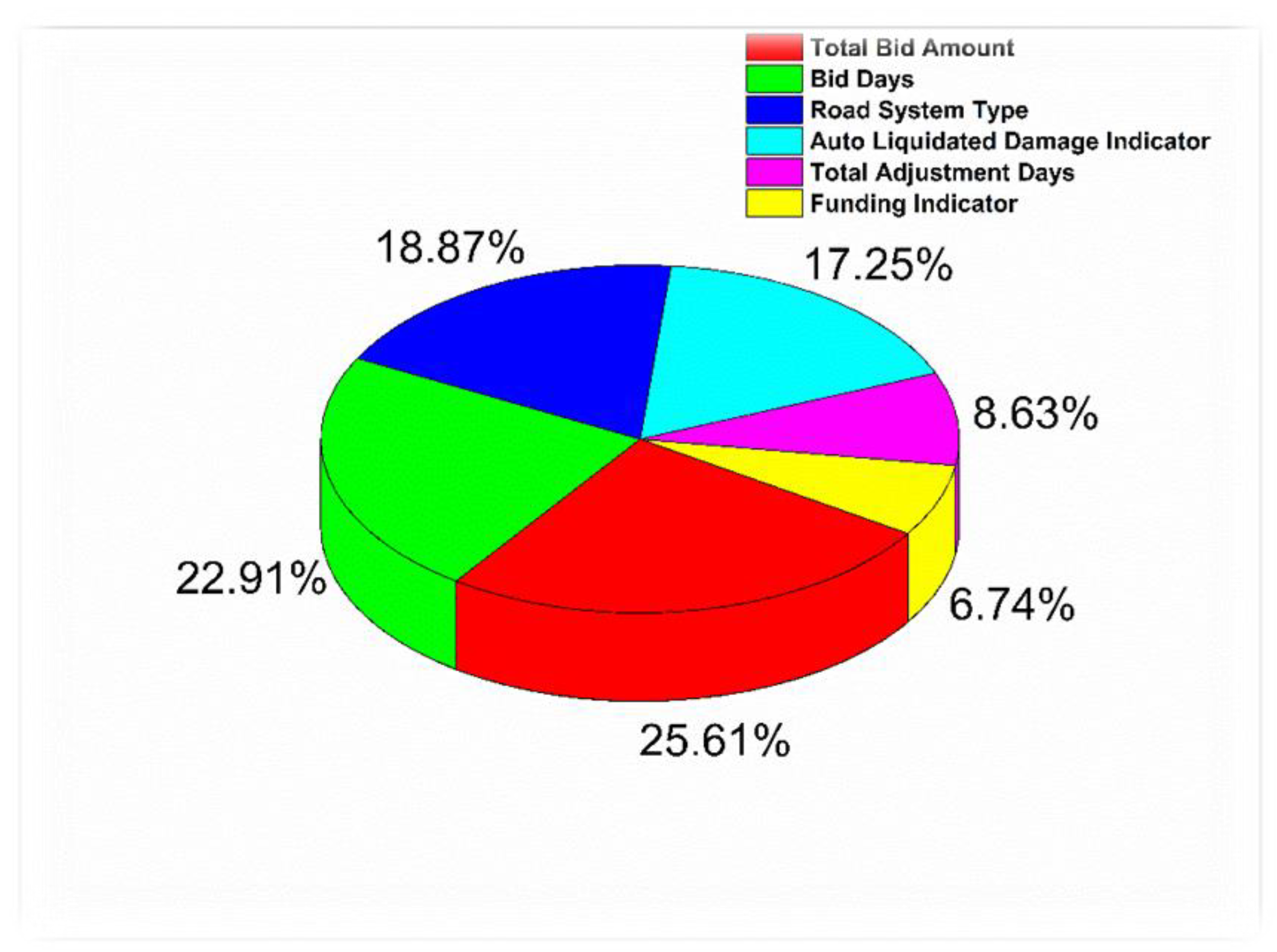
The six variables that have an acceptable impact on the prediction of $\mathrm{LDs}$ are shown in Figure 15. Again, feature importance was used to identify the most and least important independent variables. The four variables that most significantly impacted LD predictions were the Total Bid Amount, Bid Days, Road System Type, and Auto Liquidated Damage Indicator. The most important variable was the Total Bid Amount, while the least important was the Funding Indicator.

This work has shown that the proposed modified MLR model could be useful as a management decision support tool for $\mathrm{LD}$ issues. Moreover, until now, no research has studied the independent variables mentioned in this paper.

12. Practical Implications

Decision-makers have increasing confidence in technical outcomes to modernize and develop their policies. The current research builds a vigorous machine learning framework for liquidated damages predictions from the recorded datasets, which can be used in highway construction project life-cycle cost analysis. Doing so proposes a solid base for exploring the interconnectedness of these distinct features, which can be enlightening with regard to LD forecasting. Additionally, as modern machine-learning algorithms continue to evolve, expanding advanced forecast models opens a path to developing additional functional and precise modeling for LD prediction, which numerous highway building business practitioners can then employ. Conclusively, congruent to what is currently emerging in the research areas of construction engineering and management, the authors have confidence in the proposed models to offer stakeholders a more precise forecast, to better fit accessible datasets as an advantageous precondition using machine-learning-based models.

The current research aims to minimize the knowledge gap in LD prediction for highway construction projects. Thus, the proposed models were designed after an intensive investigation of the currently available related models. For example, one of the main gaps is the lack of a clear and integrated representation of how the main attributes affect the LD interconnectedness. This negatively affects LD forecasting accuracy as the main attributes are usually accompanied by high level of uncertainty [12]. Furthermore, minimal efforts have been dedicated to developing analytical or machine learning-based models for LD prediction. Many of the currently available models utilize survey and questionnaire approaches to define the state of practices concerning LDs [17]. Additionally, many researchers have highlighted that rule of thumb procedures for estimating LDs are inaccurate and are usually accompanied by time-consuming legal disputes and extensive project delivery delays [14,15,26]. Moreover, there is a gap in historical LD data, especially with regard to construction contracts that exceed twenty million USD, and the problem grows more complicated when the contract value exceeds 100 million USD [2]. Thus, it is vital to develop a prediction model that can be practically utilized regardless of the construction cost value.

The advantage of the developed LD prediction models over similar modeling approaches available in the literature is their distinctive processing chronological sequence, where forecasts are less influenced by the number of classes and can be consistently assessed. The developed models deliver a reduced number of discriminant nodes, which will gradually reduce the number of class dimensions to be estimated. With superior-performance evaluation, the developed prediction models can implement short-running models with high-level forecast precision and less memory utilization. Furthermore, compared with other available models, it was found that the developed models can be described as an effective decision support tool within various areas of the construction industry. To summarize, the proposed models can be considered integrated, generic, practical, and accurate prediction tools. Thus, the proposed models are expected to play a critical role in reducing potential conflicts between stakeholders in the highway construction industry, especially in cases where the decision-makers face major challenges and difficulties in estimating “fair” liquidated damages that all contractual parties can agree on. As a result, proposing decision-support tools with cutting-edge technologies and software is vitally required in the construction project management industry [27,28,29,30,31,32,33,34].

13. Conclusions

This paper proposed seven modified MLR machine learning models to predict Liquidated Damages (LDs). These models are regression analysis-based, exponential, quadratic, second-degree, and third-degree polynomials. The results suggest that the most substantial independent variables for predicting $\mathrm{LDs}$ are Total Bid Amount, Bid Days, Road System Type, Auto Liquidated Damage Indicator, Total Adjustment Days, and Funding Indicator.

The three most influential factors were the Total Bid Amount, Bid Days, and Road System Type. The influence of the Total Bid Amount can be explained because LDs are usually quantified as a percentage of the overall project cost. Therefore, as the total project cost increases, the LDs would be expected to increase. The influence of the Bid Days can be explained by the fact that project duration significantly influences LDs, as projects with longer durations have higher costs. Finally, the influence of the Road System Type can be explained by the fact that the road system plays a key role in determining the rules and regulations adopted by the entity that funds the project. Federal regulations must be followed when the project is a federal or interstate highway, while state regulations must be followed for state and county highways.

Total Adjustment Days could not be used in LD prediction because some of these adjustments result from change orders based on their owner requests, and developers are not held accountable for delays caused by owner requests. As a result, the impacts of such requests are extremely unpredictable.

A simple MLR model did improve LD forecasting in certain cases. However, a more complex nonlinear modified MLR model (with second-order terms) was needed for more accurate estimations. The resulting integrated prediction model is likely to be useful in forecasting LDs to support decision-makers. For example, artificial neural networks could fill the gaps where datapoints are missing. Furthermore, data collection and recording quality might be enhanced, as accurate and complete data are essential to forecast LDs correctly. Moreover, regression analysis could be based on more sophisticated machine learning techniques (e.g., Light Gradient Boosting Machine (LGBM), K-nearest neighbors (KNN), Gradient Boosting Machines (GBM), Decision tree (DT), and Artificial Neural networks (ANN), which could be developed to predict LDs automatically.