
Spatial-Temporal Flows-Adaptive Street Layout Control Using Reinforcement Learning
by
 , , , , and
Qiming Ye
* ,
,
Yuxiang Feng
,
Eduardo Candela
,
Jose Escribano Macias
,
Marc Stettler
and
Panagiotis Angeloudis
Department of Civil and Environmental Engineering, Imperial College London, London SW7 2AZ, UK
*
Author to whom correspondence should be addressed.
Sustainability 2022, 14(1), 107; https://doi.org/10.3390/su14010107
Submission received: 29 November 2021
/
Revised: 16 December 2021
/
Accepted: 20 December 2021
/
Published: 23 December 2021
(This article belongs to the Special Issue Shared Mobility and Sustainable Transportation)
Abstract
:Complete streets scheme makes seminal contributions to securing the basic public right-of-way (ROW), improving road safety, and maintaining high traffic efficiency for all modes of commute. However, such a popular street design paradigm also faces endogenous pressures like the appeal to a more balanced ROW for non-vehicular users. In addition, the deployment of Autonomous Vehicle (AV) mobility is likely to challenge the conventional use of the street space as well as this scheme. Previous studies have invented automated control techniques for specific road management issues, such as traffic light control and lane management. Whereas models and algorithms that dynamically calibrate the ROW of road space corresponding to travel demands and place-making requirements still represent a research gap. This study proposes a novel optimal control method that decides the ROW of road space assigned to driveways and sidewalks in real-time. To solve this optimal control task, a reinforcement learning method is introduced that employs a microscopic traffic simulator, namely SUMO, as its environment. The model was trained for 150 episodes using a four-legged intersection and joint AVs-pedestrian travel demands of a day. Results evidenced the effectiveness of the model in both symmetric and asymmetric road settings. After being trained by 150 episodes, our proposed model significantly increased its comprehensive reward of both pedestrians and vehicular traffic efficiency and sidewalk ratio by 10.39%. Decisions on the balanced ROW are optimised as 90.16% of the edges decrease the driveways supply and raise sidewalk shares by approximately 9%. Moreover, during 18.22% of the tested time slots, a lane-width equivalent space is shifted from driveways to sidewalks, minimising the travel costs for both an AV fleet and pedestrians. Our study primarily contributes to the modelling architecture and algorithms concerning centralised and real-time ROW management. Prospective applications out of this method are likely to facilitate AV mobility-oriented road management and pedestrian-friendly street space design in the near future.
1. Introduction
The complete streets scheme is a mainstream engineering solution to improve road sharing for all road users [1,2]. It balances all users’ public right-of-way (ROW) and canalises road proportions according to respective travel demands [3,4]. A balanced ROW through the implementation of a complete street scheme could accommodate all modes of travel with rational road shares, an efficient operational environment and safe travel experiences [5,6].
Evidence shows that the complete streets scheme has considerably contributed to reducing road hazards, especially inter-modes traffic accidents, while maintaining relatively high transport efficiency [7,8]. However, their rigid and canalised thoroughfares have been criticised by a significant proportion of planners and geographers for the imbalanced ROW assignment [9]. They have a strong belief that the complete streets scheme particularly priorities motorised mobility while diminishing the shares for active travel modes. They demand that active modes of transport and street events should be granted larger road space shares compared with the status quo [10]. This appeal deeply roots in humanitarian urbanism and profoundly underpins a storm of movements that shifts supremacy from automobiles to non-motorised users within neighbourhoods or at critical public realms [11]. This reclaim of street space represents a force that is currently reshaping complete streets through measurements like traffic calming [12], temporarily or permanently occupying driveways [13,14].
Autonomous Vehicles (AVs) and Shared Autonomous Vehicles (SAVs) are emerging as the next solution to urban mobility. A substantial number of studies have predicted their potential to transform the conventions of travel patterns fundamentally [15]. Furthermore, a significant proportion of them share concerns on such changes as exogenous challenges faced with entire road networks and complete streets [16]. They fear that the induced demand by AVs transport could overload the streets of city centres during morning and evening commutes [17]. However, the positive effects include a considerable reduction in the throughput pressure of neighbourhood roads [18], suggesting opportunities to re-balance the ROW usage among road users. Simultaneously, Pick-Up and Drop-Off (PUDO) practices of SAVs [19], fast electric charging services [20], deployment of Roadside Units (RSUs) [21] and automated logistics [22] are likely to redefine the functions of streets in the AVs era. These new street norms would foster a revolution of the ongoing complete street schemes to be more inclusive, pedestrian-aware, and flexible.
The challenges, as mentioned earlier, call for a careful rethink of the state-of-the-art design protocols of streets and the development of novel techniques to manage the road space usage in a more innovative way. With the advancement of intelligent and connected road infrastructures, real-time control over the ROW could be considered as a new engineering approach. Furthermore, assisted with artificial intelligence (AI), road traffic management has experienced significant progress, particularly traffic signal control [23,24] and traffic operations control [25]. Despite these advancements, the optimal control models focusing on the assignment of ROW are seldom present in the literature. Thus, this research was proposed to contribute to this area.
To solve this optimal control problem, we have introduced a Reinforcement Learning (RL) method, namely a Deep Deterministic Policy Gradient (DDPG) algorithm for the real-time road space assignment to corresponding road users. The goal is to realise a traffic flow-responsive and pedestrian-friendly street layout by altering the ROW proportions assigned to driveways and sidewalks. A four-legged intersection and a 24-h AVs-pedestrians combined travel plan constitute the basic modelling settings. This DDPG algorithm incorporates the open-source microscopic traffic simulator, Simulation of Urban Mobility (SUMO), for retrieving the operational AVs’ and pedestrians’ dynamics, and the states of the road environment. In addition, both symmetric and asymmetric road layouts are simulated to measure the effectiveness of the proposed method.
The contribution of this study is four-folded. First, a novel RL-based approach is proposed and validated to address the real-time ROW assignment problem, benefiting the inclusiveness and efficiency of future streets. Second, the model coordinates the seemingly conflicting objectives of place-making and transport efficiency, combining urban planning and traffic engineering appeals. Third, our model is likely to be scalable concerning measuring simple road geometries, which are generally defined by limited edges, but potentially city-level road grids. Last, as a seminal building block of the Intelligent Transport System (ITS), this proposed method could further incorporate peer controlling technologies to accommodate potential challenges raised by the introduction of AVs mobility.
2. Literature Review
This section provides a systematic review of peer studies concerning three seminal aspects. First, we surveyed the complete streets scheme, which is the most widely implemented guide for street design practices. Second, we reviewed challenges facing the implementation of this scheme. Third, essential objectives concerning streets design and management are summarised.
2.1. Public Right-of-Way of Complete Streets Scheme
In transportation, the public ROW, or the ROW of road space, defines the legal right or the priority of specific types of road users to pass along a route through the street space [1]. These road users include not only motorised vehicles, but also vulnerable groups such as pedestrians and cyclists [2]. The purposes of balancing the ROW include improving traffic efficiency, engaging all modes of transport, and reducing potential inter-mode conflicts [6].
The complete streets scheme has risen as a mainstream engineering solution to balance the ROW [3,4]. It satisfies the basic demands of accommodating all road users with corresponding shares of space, but simultaneously canalise such space as per distinctive modes of travel [5,6]. The complete streets scheme principally comprises a driveway zone and a streetside zone. Figure 1 demonstrates four examples of its ROW plan.
Both the driveway and streetside can be further subdivided into different functional sections [26]. For instance, a driveway zone comprises several driving and curb lanes (Z), and possibly a median (Z). Meanwhile, a streetside sits between the driveway and private lands, primarily serving non-vehicular mobility and providing accessibility to venues, comprising cycle lanes (Z) and sidewalks (Z). It also includes a variety of road facilities in facility belts (Z), and lively street activities in the front zones (Z) [9,27].
Due to differences in street functions, locations and throughput capacities, the sectional widths vary significantly [9]. On one hand, roads can be categorised into four types according to their functions: commercial, residential (lanes, mews), landscape (boulevard, parkway) and trafficking. On the other hand, concerning their serving capacity, the ROW can be classed into four grades: main roads, secondary roads, branches, and laneways [28]. For instance, boulevards are landscape-functional main roads, and the commercial avenues are commercial-oriented main roads [29].
Based on a holistic survey of the state-of-the-art available complete streets scheme worldwide, we compared and summarised the following underlying principles of designing a street. First, the sidewalk should be planned no less than 1.5 m, and it is encouraged to be between 2 m and 2.5 m for new development residential streets or downtown commercial streets [27,28,29,30]. Second, the width of a driving lane is considered 3 m to 3.5 m for passenger cars, freight vans and trucks in urban areas. Third, a curb lane is suggested to bear a width of 3 m for on-street parking operations [27]. Fourth, the provision of cycle lanes can be flexible as it could occupy an independent lane with a width between 1.5 m to 2.5 m; Alternatively, driving lanes could accommodate those cycling demands. Fifth, the comprehensive facility belt should at least be assigned with 1.5 m to 2 m in width [27,28]. Finally, any street should secure a clear path in a width of 3.5 m to ensure the operations of emergency vehicles.
2.2. Challenges Facing Complete Streets Scheme
It is widely acknowledged that the complete streets scheme has achieved seminal contributions with regards to road safety and the operational efficiency of traffic flows [7,8]. However, these rigid and canalised patterns handicap their flexibility and resilience in responding long term’s endogenous and exogenous challenges facing road space.
The endogenous challenges emerge from the priority of usage between vehicles and the other modes of travel. A wide range of planners and geographers have criticised the complete street as ’incomplete plans’ concerning streets as public space [10]. They claimed that street events, pedestrians, e-scooter riders and cyclists should be granted more space than and priority to cars [11]. Temporary measurements, such as closure of driveways in a short period of time [13], and some permanent remedies, like traffic calming [12], shared road surface [31] have firmly responded to such appeal. The recent Covid-19 pandemic also fostered the reclaiming of driveways for non-vehicular traffic operations or as extensions of indoor activities [14]. To take placemaking and urban design into account, such flexibility of road space usage could potentially support diverse street activities and reinforce the public recognition of streets as public space [32].
The prominent exogenous challenges could be the deployment of Autonomous Vehicles (AVs) and Shared Autonomous Vehicles (SAVs) mobility [33]. It is expected that the future urban mobility and goods logistics could be replaced almost entirely by these disruptive modes of transport around 2040 to 2060 [34]. One of the early research jointly conducted by the Boston Consulting Group (BCG) and the World Economic Forum (WEF) found that with a moderate 60% of market penetration, AVs mobility might induce considerable trips to downtown areas during the morning and evening commute peaks. This could overload streets of city centres, raising travel costs by at least 5.5%, while broadly alleviating traffic in suburban neighbourhoods by 12% [18].
An increasing proportion of studies on AV transport demonstrates the disruptive impact of SAVs, which may transform our current transport into the Autonomous Mobility-on-Demand (AMoD) system [35]. By adopting SAVs, it is estimated that 16% of current vehicular fleet could suffice daily mobility [36]. While 85% of current off-street parking space land can be liberated [37], while frequent Pick-Up and Drop-Off (PUDO) events would require more curb parking areas to be installed and efficiently managed [19]. In addition, some emerging new road infrastructures, including the rapid charging facilities, may also disrupt the conventional street functions and demand for new spatial plans to accommodate new ROW desires [20,33].
These potential changes signal the urgency to revisit the current design protocols and renovate road management techniques. With the promising advancement of intelligent and connected road infrastructures, real-time optimal control over ROW might present a novel solution to this problem. Although new methods and algorithms have been developed, with some even tested on roads [38,39], those pioneering practices are still confined within limited road infrastructures, such as traffic signals and roadside units [21,40]. Moreover, the status-quo models and algorithms still fall far short in supporting the dynamic control of public ROW.
2.3. Performance Metrics Regarding Street Design and Management
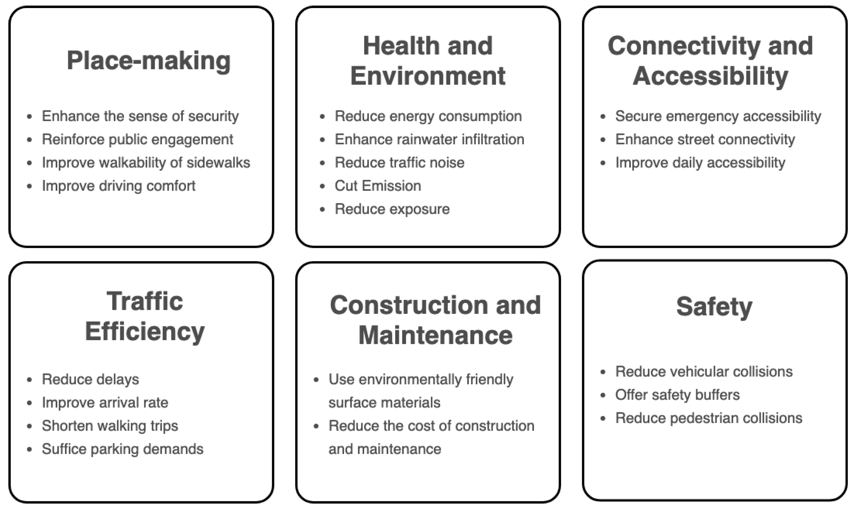
Good street space is underpinned by objectives from a broad spectrum of domains [9]. In other words, the design and management of streets usually correspond to a multi-objective decision-making process given a collection of goals [41]. These domains include place-making, health and environmental, connectivity and accessibility, traffic efficiency, construction and maintenance, and safety [9,41], as summarised in Figure 2.
Regarding our study, we first treat users’ safety as the baseline. Namely, the requirement of collision-free was encoded as a priority in our model. Then, among the rest objectives, we approach to balance place-making and transport efficiency, hoping to coordinate traffic engineering and urban planning appeals. On the one hand, evidence proves that suffice the territory of sidewalks can effectively enhance the safety perception of pedestrians, contributing to more comfortable walking experiences, and simultaneously engaging street lives [9,10,12]. On the other hand, the operational efficiency represents a significant indicator measuring the primary trafficking performance of roads [42].
2.4. Summary of Literature Review
The essence of designing the road space is to engage all modes of transport and ensure their travel safety and traffic efficiency. As a prevalent solution to this engineering problem, the complete streets scheme canalises road space per distinctive modes of travel to accommodate all road users. However, despite the ensured traffic safety and efficiency, the complete streets scheme presents a lack of flexibility and resilience concerning challenges introduced by AV mobility. In addition, such a solution is yet balanced enough to echo the demands for truly pedestrian-friendly road space.
Traffic engineers, urban designers, and planners need to cooperate in upgrading the current street design protocols and renovating road management techniques for a flexible, human-oriented ROW control scheme. To the best of our knowledge, the status quo literature probed into limited solutions to traffic signals control problem and roadside units control problem while offering no clear methodology, either theoretically or practically, to the ROW control problem concerned by our study.
3. Preliminaries of Reinforcement Learning
3.1. Reinforcement Learning and Markov Decision Process
Reinforcement Learning (RL) represents one of the cutting-edge branches in Artificial Intelligence (AI) methods. It includes a wide range of popular algorithms that address optimal control problems via a trial-and-error procedure [43]. Concretely, intelligent agents embedded with RL controllers learn optimal policies to interact with the environment and take actions. They retrieve feedback and update their decision-making machinery for higher scored movements in the subsequent attempts [44]. RL has been widely applied in solving real-world problems such as robot control, dispatch management problem, the Travel Salesman Problem (TSP) and production scheduling problem [45]. Furthermore, it has been intensively practised in transportation studies for traffic signal control [23,24,38], vehicles routing [46], movements control [47] and traffic operations control [48].
By convention, a control problem could be defined using a Markov Decision Process (MDP), denoted as a tuple . N is the number of agents in the MDP, and an agent is indexed by . Agents interact with the stochastic environment and observe the states. Let define the joint state space, where each state element indicates a high-dimensional state space. Let T be the time horizon, the component state-space comprises individual observation of agent n at time step , herein . Similarly, defines the joint action space. A state-action space describes a trajectory of agent-environment interaction, which is expressed as . Given a trajectory , P defines a stationary transition probability of being in a state s given an action a at time t and transforming to the next state at time . Let defines the immediate reward from the environment once the agent observed state s and take the action a. The controlling objective is to maximise the cumulative reward of all agents from to the temporal limitation. Here, is a discounted factor representing the decaying contribution of the expected immediate reward.
3.2. Deep Deterministic Policy Gradient (DDPG) Algorithm
Policy Gradient (PG) algorithms represent a vital branch of RL methods that address optimisation problems characterised by a continuous action space [49,50]. Let define a stochastic policy that executes an action a observing a state s, and represents the probabilistic distribution of taking this action under such policy.
The Stochastic Policy Gradient (SPG) algorithm is an early representative of PG algorithms. The discounted future reward of SPG at time t with a discount factor is expressed as following Equation (1). Whereas Equations (2)–(4) present the state value function, state-action function and advantage function of SPG respectively. SPG conducts a gradient ascend approach to optimise the policy parameter , which is expressed in Equation ().
The deterministic policy gradient (DPG) method approximates the optimal policy using a deterministic policy rather than the random approach adopted by SPG. In other words, DPG is a ’limiting analogue’ of the stochastic counterpart, according to its theorem [51]. Let indicate the deviation corresponding to the probabilistic distribution . As Equation (6) expresses, DPG is the condition where . DPG can either be modelled in an on-policy or off-policy way. An on-policy DPG usually requires a large number of samples for learning [52]. Instead, an off-policy DPG is self-sufficient regarding training samples because of the embedded perturbation mechanism.
The Deep Deterministic Policy Gradient (DDPG) algorithm is a model-free off-policy DPG, which inherits features from both DPG and Deep Q-network (DQN) [53]. Namely, it embeds deep neural networks to enable an end-to-end learning ability [54]. The DDPG has improved significantly from three aspects in comparison with DPG and DQN. First, an exploration policy that generates random noises is implemented in DDPG to suffice exploration. Second, an experience replay buffer trains neural network parameters in an off-policy manner. Third, conventional DQN updates the target action-value function through periodically coping from the current action-value function Q. In contrast, DDPG updates its parameters of both target networks at each iteration and proportionately at a soft update rate .
4. Methodology
In this section, we first formulate this dynamic ROW assignment problem as an optimal control problem. Our proposed solution model combines the SUMO traffic simulator and a DDPG algorithm. Then, a detailed explanation is provided covering the state, action, reward, experience replay buffer and essential parameters of the actor-critic architecture of DDPG.
4.1. Modelling Formulation
Consider a simple network represented by a bi-directed graph , where denotes the width of an edge and indicates the width of a facility belt. Let be the proportion of a driveway. As such, the width of the driveway equals , whereas the counterpart streetside has a width of (. Figure 3 highlights the spatial relationship among these variables, given a ROW plan of an edge. Provided a consecutive pair-wise AV traffic demands and pedestrian travel demand at , the problem is to optimise the driveway ratio of discrete edge and at each time slot, to improve travel efficiency of road users and a higher ratio of sidewalks.
Table 1 demonstrates the notation conventions applied for the formulation of this optimal control problem. Following previous studies [55,56,57,58], we consider the following physical parameters for the simulation: the maximum operational speed and maximum acceleration of an AV are 13 m/s and 2.6 m/s2, respectively. The vehicular length is set at 4.5 m. Pedestrian walking speed is limited to under 1.2 m/s to ensure the testing scenario for intersections.
Our objective function (7) is composed of three sub-objectives which are expressed in Equations (8)–(13). Namely, at each time slot t, the objective maximises reward from vehicular traffic efficiency , pedestrian traffic efficiency and sidewalk ratio . Here, an amplifier is applied to scale the total objective .
Equation (8) presents that equals the ratio between the free-flow travel time and the actual travel cost , where indicates the total traffic delay of the fleet in time slot t. Equation (9) estimates that as a sum of travel costs of all AVs operating at their respective maximum speed in the system. Equation (10) expresses that the traffic delay equals the gap between the integral of the arrival rate and that of the departure rate. In this equation, and represent functions of the arrival rate and the departure rate controlled by time t given .
The calculation of the pedestrian traffic efficiency follows a similar rule as that of , as described in Equation (11). The individual free-flow walking time and pedestrian traffic delay are acquired following Equations (12) and (13). Following Equation (14), the third sub-objective component maximises the cumulative sidewalk ratio, namely , at time t of edge e. Here, indicates the width of the facility belt.
The problem is constrained by Equations (15)–(24). Constraint (15) requires that the distribution of operational speed of the fleet to follow a normal distribution, which has a mean of 13 m/s multiplying a speedFactor = 1.0, and a deviation = 0.05. Constraint (16) sets the upper bound of the real-time speed of an AV, expressed as , which should not exceed the designated operational rate. Let indicate the acceleration of an AV at t, Constraint (17) limits this acceleration as below 2.6 m/s2. Let () and () denote the coordinates of an AV and pedestrian respectively, where V and P. Constraint (18) demands the minimal longitudinal distance of the proceeding car to suffice the clearance gap requirement. Constraint (19) further estimates such clearance gap using time headway h, the mean velocity of the two vehicles and vehicle length .
We apply similar constraints on the simulation of pedestrian dynamics. Concretely, Constraint (20) regulates that the real-time velocity of a pedestrian be bounded by the maximum speed 1.2 m/s. Constraint (21) ensures that the acceleration of a pedestrian at t should not exceed 0.3 m/s2. In addition, Constraint (22) defines a minimal inter-person space as the norm of the vector between two pedestrians , in which equals 0.25 m in this study.
The hourly flow rates of AV transport and pedestrians are generated in alignment with the bimodal travel time distributions, following the description in [59]. A travel plan jointly synthesises pedestrian trips and AVs trips at the OD-pair level in 48-time slots of a day. Let and denote the vehicular and pedestrian travel demands per OD pair at time t. The sizes of AV fleets and pedestrians subject to corresponding travel plans, as expressed in Constraints (23) and (24).
Constraint (25) describes the boundaries assigned to the decision variable. Its lower limit represents the edging case where only one emerging lane is reserved, and the upper bound ensures the extra provision of at least 1.5 m sidewalk. Constraint (26) determines the number of lanes regarding and . The final condition corresponds to the case of the multi-driving lane.
4.2. SUMO Traffic Simulation Incorporated DDPG Modelling Framework
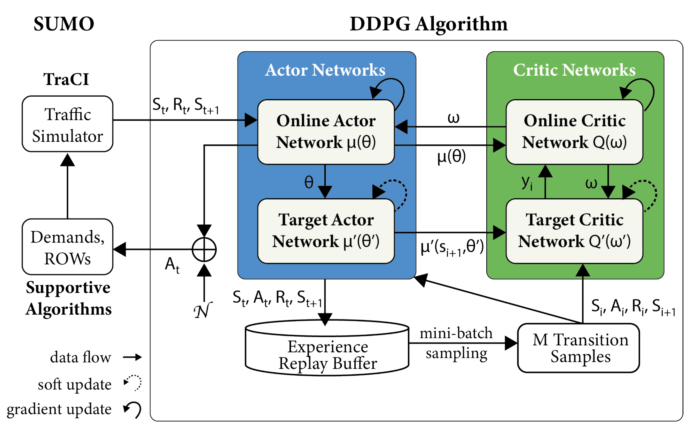
We proposed a SUMO-incorporated Deep Deterministic Policy Gradient model to address this optimal control problem, namely the SUMO-DDPG. Figure 4 presents the modelling framework, which essentially comprises two interactive components: a SUMO traffic simulator and a DDPG controller. Initially, SUMO generates network configurations using default ROW settings. It also generates discrete vehicular and pedestrian trips according to the pre-defined travel plans. Then, we use the Traffic Control Interface (TraCI), a SUMO built-in API, to calibrate road geometries at each time slot and acquire states of all AVs, pedestrians and environments.
The DDPG algorithm comprises an actor-critic model and an experience replay buffer. First, the actor-critic model consists of four neural networks: an actor online network , an actor target network , a critic online network and a critic target network . Here, we use , , and to indicate the parameter sets of these four neural networks, respectively.
This DDPG is trained in 150 episodes and at the edges level, meaning discrete edges make individual decisions. One training episode comprises a number of time slots bounded by the starting time slot and 3600 s. Each time slot is equivalent to a length of min in the real world.
Meanwhile, the DDPG controller interacts with SUMO via TraCI at an interval of s, namely 50 visits in a single slot. During the interactions, a set of edges evaluates the environment state (), executes a collection of individual actions (), receives a joint reward (), and observes a future environment state (). This information is then utilised to update the neural network parameters of the actor-critic model.
4.3. DDPG Algorithm Structure
The following subsection details the state, action, reward, experience replay buffer, and parameters applied for both actor and critic networks. Table 2 lists the key hyper-parameters concerned by our SUMO-DDPG model.
4.3.1. State
The observed state includes the number of operational AVs and pedestrians on each edge. Let denote this two-dimensional state vector per edge, , whereas and indicate the real-time operational numbers of AVs and pedestrians on edge e. Thus, at a time slot t, the joint state space is defined as .
4.3.2. Action
The action taken by an edge e at time step t is denoted as , representing the proportion of the link occupied by the driveway. Note that the action space of is continuous in a range of . Thus, the joint action space for the whole system is expressed using a -dimensional vector . Equation (27) expresses that the actor online network determines a deterministic action following the policy .
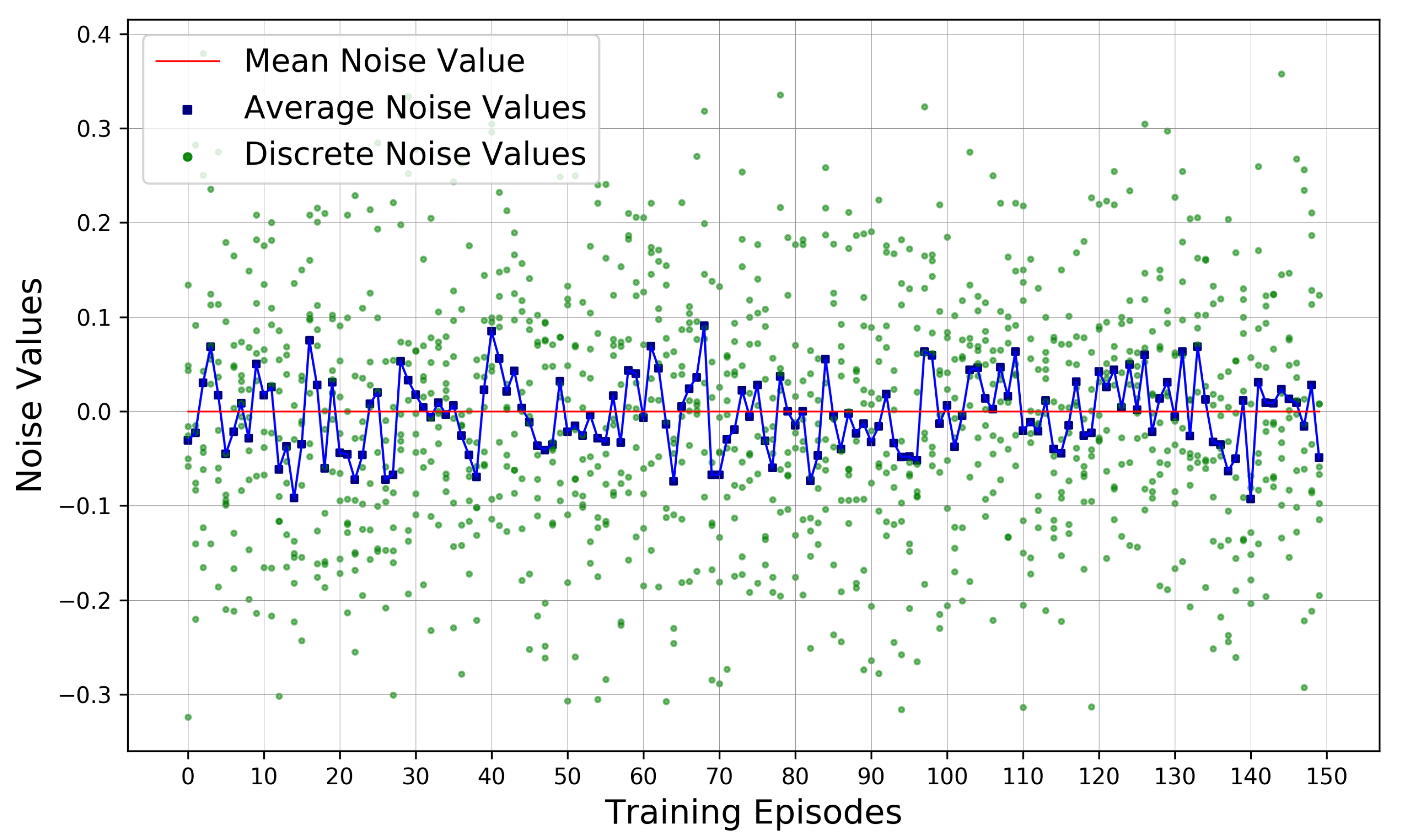
Equation (28) presents an Ornstein–Uhlenbeck process that generates a time-dependent noise to sufficiently explore the action space. By convention, it usually comprises a Gauss–Markov procedure and a white noise perturbation [60]. The Gauss–Markov noise distribution is defined by its mean , the regression rate to its mean and a standard deviation . The white noise is modelled as , which describes a normal distribution with a mean of and a standard deviation of 0. Following that, Equation (29) expresses the eventual joint action taken by edges, which equals the sum of the deterministic part and the value of noise.
Figure 5 presents a record of the obtained Ornstein–Uhlenbeck noises from eight tested discrete edges (green dots) and their average value per episode (blue squares). The horizontal red line highlights that mean noises fluctuate around 0.
4.3.3. Reward
A reward quantifies the feedback from the environment to evaluate an executed action [44]. In this current study, this reward is estimated using the value of following specific rules as explained in Formula (30). This formula regulates that this reward is 0 if more than one of the following illegal occasions happens: (1) the value assigned for decision variable exceeds either limit; (2) uncompleted trips due to disconnected routes. For instance, if a person could not complete the assigned trip from o to d due to an unconnected sidewalk-crossing system, then this reward equals 0.
4.3.4. Experience Replay Buffer
An experience replay buffer stores past transition tuples , , , for further off-line learning. A random m-sized mini-batch is randomly sampled from the buffer to feed both target networks in the off-line learning process. Then a transition trajectories for learning is denoted as , , , , where index samples of mini-batch.
4.3.5. Actor Networks
The actor online network approximates to the optimal policy by minimising the gradient loss of . The corresponding loss function and the optimisation function for updating the gradients are described in Equations (31) and (32) respectively.
The actor target network updates the network parameter using a soft update strategy controlled by a specific parameter , following Equation (33).
4.3.6. Critic Networks
The target part of critic networks estimates a target Q value . Then, following the Bellman Equation [61], it sums the sampled reward and a discounted future state-action values using the network policy parameter and a discount factor , as expressed in Equation (34). In parallel, the critic online network first calculates the Q value and then updates parameter by minimising the gradient loss between and this Q value. Equations (35) and (36) express this loss function and gradient update approximation respectively.
The critic target network updates its parameter controlled by following Equation (37).
4.3.7. Keras Neural Networks
Both actor and critic networks were implemented in Keras. An actor network comprises two hidden layers, which inputs a -sized observed states layer and outputs -dimensional actions. The rectified linear activation function (ReLU) and tangent activation function (TanH) are implemented as calculation rules for the input and output layers respectively.
A critic network has six hidden layers in total. Initially, a -sized state layer and -dimensional action layer are input as dual-sourced layers. Then, both layers are activated using ReLU and later concatenated as a joint layer. Finally, the eventual output layer is featured in the size of for the control task of each edge.
5. Model Training and Results
5.1. Specification of Travel Plans and Testing Case
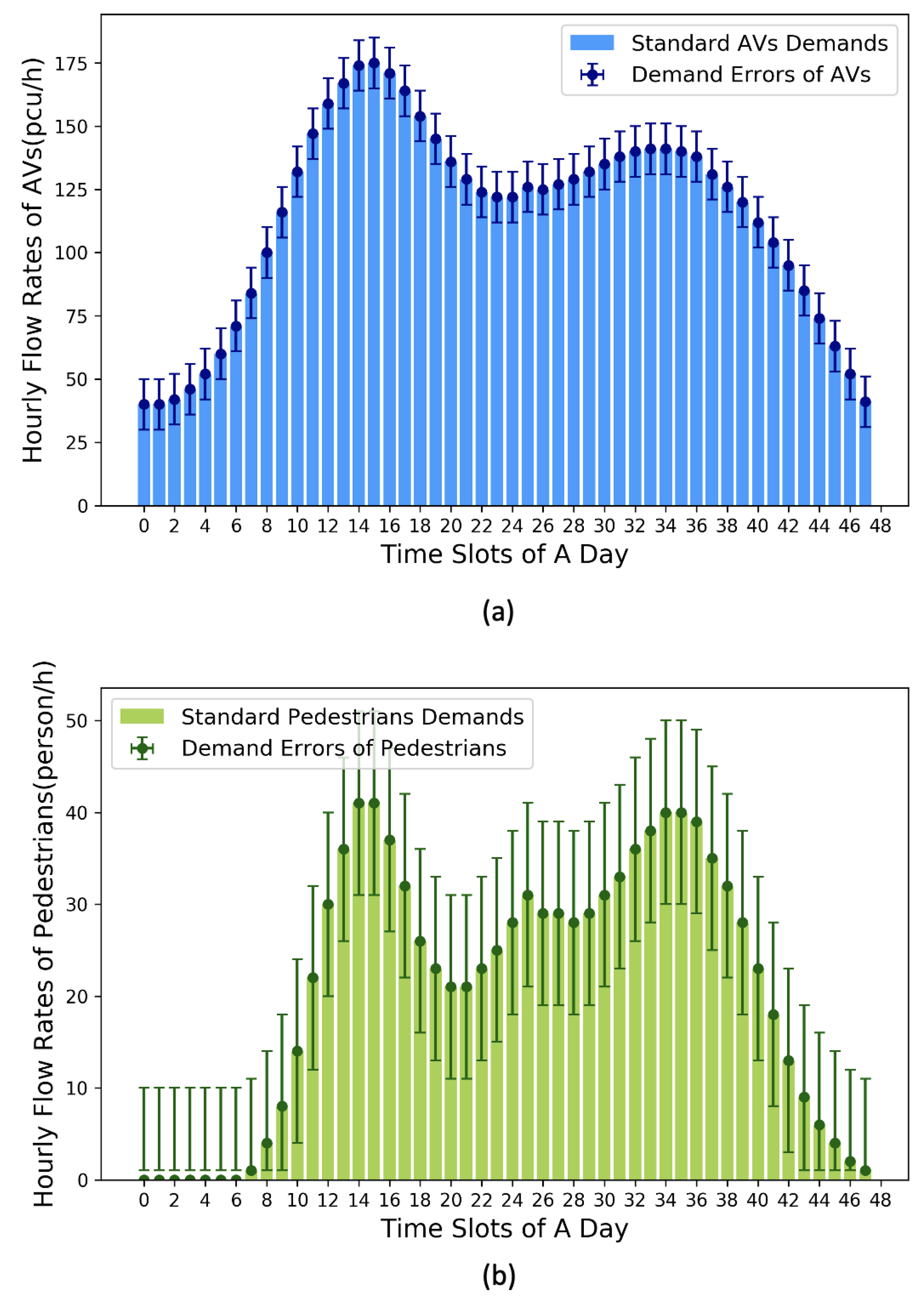
Figure 6 demonstrates the OD-pair based travel demands at 48-time slots, with error marks representing stochastic perturbations (±10 puc/h or person/h) based on their respective mean demands.
The mean OD-pair level travel demands of AVs and pedestrians are 114 pcu/h and 21 person/h respectively. Concretely, two peaks of AVs traffic flow appear at 07:30 (175 pcu/h) and 18:00 (140 pcu/h). Meanwhile, pedestrian flow rates reach the highest demands at 07:30 (41 person/h) and 18:00 (40 person/h).
The prototypical road layout for testing originates from a four-legged intersection. This road layout has four 100 m roads comprising eight connected edges, . We have further calibrated this prototype into one symmetric layout case and an asymmetric case to ensure the usability of our proposed SUMO-DDPG model under varied geometric conditions.
The symmetric case has homogeneous edge widths, namely [16, 16, 16, 16, 16, 16, 16, 16 (m)], whereas their facility belt are in the widths of [1.5, 1.5, 1.5, 1.5, 1.5, 1.5, 1.5, 1.5 (m)]. For the asymmetric case, the edge widths are [14, 14, 16, 16, 18, 18, 14, 14 (m)], which are heterogeneously configured. The widths of their facility belts are [1.5, 1.5, 1.5, 1.5, 2, 2, 1.5, 1.5 (m)]. Figure 7 demonstrates the configuration of two settings in SUMO simulation environment.
Different geometric settings lead to distinctions in the upper and lower bounds of . Despite the variations, a uniform randomness seed is shared throughout the training course over two cases. This arrangement ensures that travel plans, perturbation noises, and actor-critic models’ initial parameters are identical for both cases.
5.2. Training Performance of SUMO-DDPG
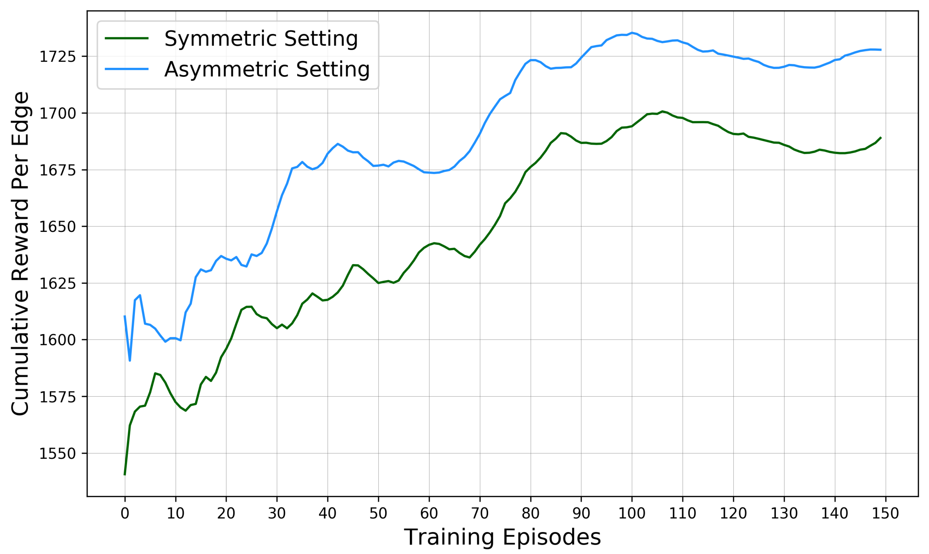
Figure 8 demonstrates the training performances of learning curves obtained from the two tested cases. The X-axis index 150 training episodes, while Y-axis represents the edge-level accumulative average reward. The blue and green curves log the generally ascending trends of such rewards obtained from the symmetric and asymmetric cases.
The reward in the symmetric case has increased by 10.39% since the initial episode. It reaches the peak of 1700.65 at an incremental rate of +1.07/ep. The learning curves of three training stages–the early stage (Ep. 0–49), middle stage (Ep. 50–99) and later stage (Ep. 100–149), present distinctive convergence patterns.
The early stage records a significant surge from 1540.61 to 1632.82, leaping a gap of 92.20 with an incremental rate of +1.84/ep. Its mean and standard deviation are 1599.26 and 22.45, indicating a rapid convergence process. In the middle stage, the reward gap drops by 68.67, from 1624.97 to 1693.63, while its standard deviation slightly rises to 24.30. Additionally, the mean reward value situates at 1660.21, with the incremental rate declines to +1.37/ep. In the last stage, the reward pattern reaches a plateau marked by the lowest standard deviation (6.15), the even narrowest mean value (18.42) and the slowest incremental rate +0.37/ep. This stage-wise declining tendency suggests the approximation to the optima.
Accordingly, the learning curve of the asymmetric case demonstrates similar convergence patterns. It has a general 9.09% in reward surge at an average incremental rate of +0.96/ep. The lowest reward (1590.73) is obtained at Ep.2, while the highest reward (1735.33) at Ep. 100. Examined stage-wise, the corresponding average reward gaps of the three stages are 95.60, 60.92 and 15.48, whereas the incremental rates are +1.91/ep, +1.22/ep and +0.31/ep. Their standard deviations are 30.24, 22.61, and 4.5. These figures signal that the obtained reward is approximate to the optima, which is consistent with that of the symmetric case.
In general, both learning curves display synchronised and incremental patterns throughout their independent training courses. These patterns evidence the effectiveness of the model as input arbitrary road geometries.
The training pattern of the symmetric case has a slightly lower episodic reward (40.01/ep) than its asymmetric counterpart, indicating a moderately better convergence performance of our model on optimising the asymmetric road layout. However, rewards of the symmetric case outperform the asymmetric ones concerning the overall reward growth rate (+1.30% higher) and the stage-wise incremental rate (+0.11/ep higher). Furthermore, despite the differences, the rewards gap of the two cases narrows down from 69.57 at Ep.0 to 38.89 at the last episode, with a mean gap of 40.01. These facts evidence that our proposed SUMO-DDPG model could effectively optimise ROW plans under symmetric and asymmetric road layout conditions.
5.3. Improved ROW Assignment Strategies
As another performance metric of our model, we would like to understand to what extent has our proposed model optimised the executed actions throughout the training course.
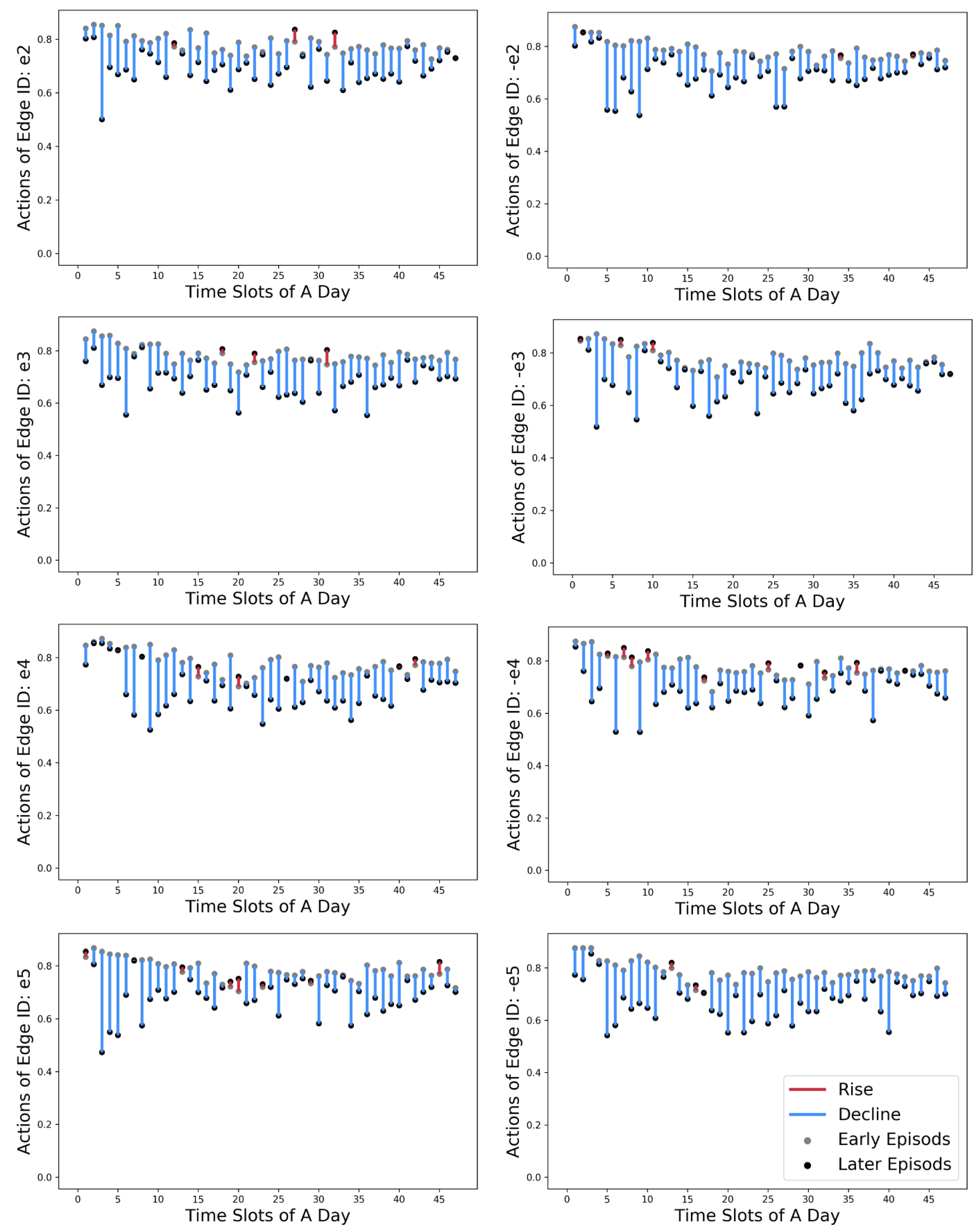
Figure 9 contains eight graphs to demonstrate the transformations of ROW decisions for each edge between their early stage and later stage. The X-axis indicates the time slots of a day, and the Y-axis shows the action values, namely the road proportion assigned for driveways (). The early-stage actions are highlighted in grey dots, while their later counterparts are in black. We use blue and red vertical bars to indicate the tendency of declining or rising in action values.
Consequently, a majority (90.16%) in action values decline, with only 9.84% showing a slight increase. The time slot-wise differences are not apparent due to these principal trends of reduction. Combined with the rising patterns of learning curves, the declination in action values suggests that our model can effectively alter the road proportions assigned to driveways to sidewalks. Such efforts in re-balancing the ROW between the driveways and sidewalks reinforce as controllers receive higher rewards from the environment feedback.
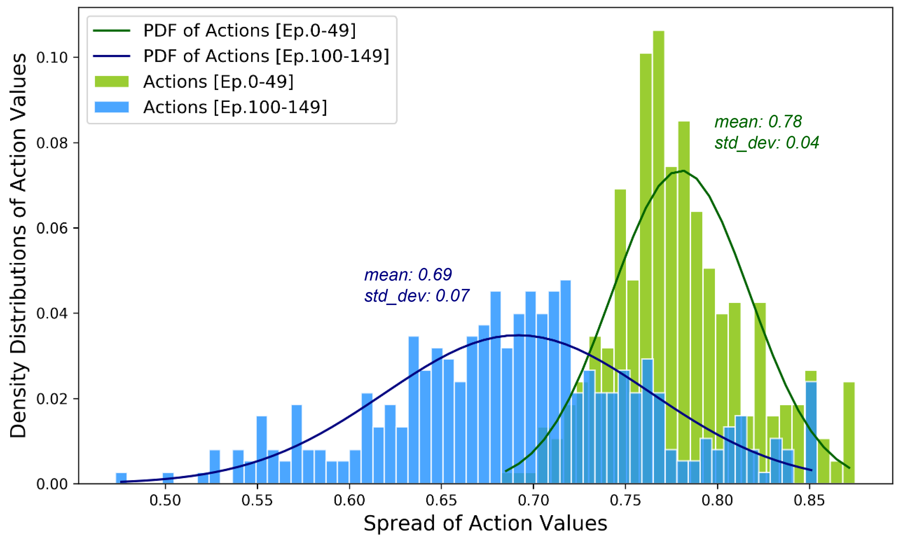
We further examined detailed transformation in distributions of actions. Figure 10 demonstrates the density distributions and their corresponding Gaussian Probability Density Functions (PDF). Optimised by our model, the actions’ density distributions get flattened throughout the training course. Their mean value transforms from 0.78 in the early stage to 0.69, shifting away from the upper limit and approaching towards the lower bound.
The road space assigned to the driveway reduces by 9% on average, namely 1.26 m, 1.44 m or 1.62 m corresponding to edges in widths of 14 m, 16 m or 18 m respectively. Additional space assigned to sidewalks is beneficial to relieve the pressure of pedestrian traffic while potentially encouraging street activities. More street activities are likely to induce demand for pedestrian flows at certain levels, requiring control models, like ours, to be deployed to manage road space assignment dynamically.
Another critical change is the notable increase in standard deviations, which has increased by 1.75 times from 0.04 during the early stage to 0.07 at the last stage. This shift indicates an even wider spread of actions after optimisation. Moreover, it provides a larger strategy pool of optimal actions to realise a more flexible, responsive and pedestrian-friendly mode road layout.
Compared with the conventional complete streets scheme, both the early and later phases liberates road space assigned for the driveways to sidewalks. At the early stage, approximately a standard lane-width (3.5 m) equivalent space is re-assigned to the sidewalk in one out of 48 time slots, of which the probability estimates 2.08%. By optimisation, this ratio significantly rises to 9 out of 48 (18.22%) in the later stage. This improvement demonstrates that our SUMO-DDPG model has effectively learnt to allocate fewer proportions to AVs trafficking while increasing the share of sidewalks under different traffic conditions of a day.
6. Conclusions
In this current study, we proposed a SUMO traffic simulator-incorporated Deep Deterministic Policy Gradient Algorithm (SUMO-DDPG) to realise the optimal control of the ROW plan. The modelling objective maximises the edge-based traffic efficiency of both AVs fleet and pedestrians while maximising the ratio of sidewalks.
This proposed model has been trained in 150 episodes using a four-legged intersection. The synthesised travel plans include OD pair-based travel demands of AVs and pedestrians. Training results demonstrate that our model is efficient in convergence to optima under both the symmetric road geometries and the asymmetric settings.
Throughout the training course, episodic rewards increase by 10.39%. Meanwhile, 90.16% of the edges reduce the driveways supply and raise their sidewalk ratios. During 18.22% of all simulated time slots, additional lane-width space is shifted from driveways to sidewalks while maintaining high standard traffic efficiency. The ROW layout solutions expand 1.75 times given arbitrary traffic patterns, contributing to more flexible, responsive, and active mode friendly road layout strategies.
A key strength of this research lies within the fact that our model coordinates the multi-objectives from both fields of traffic engineering and urban planning. This SUMO-DDPG modelling framework successfully resolved the synchronical ROW assignment optimisation problem facing multiple roads conditions in real-time. Furthermore, the centralised training and distributive actions execution accelerate the learning process while decreasing computational cost, which seems quite promising to be applied to address such ROW optimal control problem on a city-level network scale.
However, some limitations of this initial study should also be acknowledged. On the one hand, the presented testing samples could only represent a limited range of traffic conditions, whereas more testing scenarios are expected. On the other hand, the efficacy of using a centralised training machine compared to a distributed one is yet to be answered. We also acknowledge that a wide range of urban design concerns could be measured and quantified as our training objectives, targeting a sustainable street space. Despite these limitations, the methodology is original and proved effective to solve the public ROW assignment problem. Meanwhile, findings present essential insights to both road infrastructure management and urban design.
Following this preliminary study, our further research plan will focus on (1) Real urban setting-based experiments using this model. (2) Comparison among a broad spectrum of reinforcement learning algorithms that can be implemented into the control model, including distributively architect DDPG, Q-learning and Asynchronous Advantage Actor-Critic (A3C). (3) Incorporate this ROW optimal control method with other intelligent transport control techniques such as traffic signal control and roadside unit management.
Author Contributions
Conceptualisation: Q.Y. and P.A.; Methodology, Coding and Analysis: Q.Y. and Y.F.; Writing and review: all co-authors; Project Supervision: P.A., M.S. and J.E.M. All authors have read and agreed to the published version of the manuscript.
Funding
The APC was funded by the Imperial College London Open Access Fund.
Institutional Review Board Statement
Not applicable.
Informed Consent Statement
Not applicable.
Data Availability Statement
Data sharing not applicable.
Acknowledgments
We would also like to thank the Transport Systems & Logistics Laboratory at Imperial College London for enabling us to utilise their computational capacity and relevant facilities.
Conflicts of Interest
The authors declare no conflict of interest.
Abbreviations
The following abbreviations are used in this manuscript:
| ROW | Right-of-Way |
| AV | Autonomous Vehicles |
| RL | Reinforcement Learning |
| MDP | Markov Decision Process |
| DPG | Deterministic Policy Gradient method |
| DDPG | Deep Deterministic Policy Gradient algorithm |
| SUMO | Simulation of Urban Mobility software |
| OU | Ornstein–Uhlenbeck |
References
- Prytherch, D.L. Legal geographies—Codifying the right-of-way: Statutory geographies of urban mobility and the street. Urban Geogr. 2012, 33, 295–314. [Google Scholar] [CrossRef]
- Shinar, D. Safety and mobility of vulnerable road users: Pedestrians, bicyclists, and motorcyclists. Accid. Anal. Prev. 2011, 44, 1–2. [Google Scholar] [CrossRef] [PubMed]
- Slinn, M.; Matthews, P.; Guest, P. Traffic Engineering Design. Principles and Practice; Taylor & Francis: Milton Park, UK, 1998. [Google Scholar]
- Donais, F.M.; Abi-Zeid, I.; Waygood, E.O.D.; Lavoie, R. Assessing and ranking the potential of a street to be redesigned as a Complete Street: A multi-criteria decision aiding approach. Transp. Res. Part A Policy Pract. 2019, 124, 1–19. [Google Scholar] [CrossRef]
- Hui, N.; Saxe, S.; Roorda, M.; Hess, P.; Miller, E.J. Measuring the completeness of complete streets. Transp. Rev. 2018, 38, 73–95. [Google Scholar] [CrossRef]
- McCann, B. Completing Our Streets: The Transition to Safe and Inclusive Transportation Networks; Island Press: Washington, DC, USA, 2013. [Google Scholar]
- O’Flaherty, C.A. Transport Planning and Traffic Engineering; CRC Press: Boca Raton, FL, USA, 2018. [Google Scholar]
- Mofolasayo, A. Complete Street concept, and ensuring safety of vulnerable road users. Transp. Res. Procedia 2020, 48, 1142–1165. [Google Scholar] [CrossRef]
- Dumbaugh, E.; King, M. Engineering Livable Streets: A Thematic Review of Advancements in Urban Street Design. J. Plan. Lit. 2018, 33, 451–465. [Google Scholar] [CrossRef]
- Desai, M. Reforming Complete Streets: Considering the Street as Place. Ph.D. Thesis, University of Cincinnati, Cincinnati, OH, USA, 2015. [Google Scholar]
- Loukaitou-Sideris, A.; Brozen, M.; Abad Ocubillo, R.; Ocubillo, K. Reclaiming the Right-of-Way Evaluation Report: An Assessment of the Spring Street Parklets; Technical Report; UCLA: Los Angeles, CA, USA, 2013. [Google Scholar]
- Ewing, R.; Brown, S.J. US Traffic Calming Manual; Routledge: London, UK, 2017. [Google Scholar]
- Wolf, S.A.; Grimshaw, V.E.; Sacks, R.; Maguire, T.; Matera, C.; Lee, K.K. The impact of a temporary recurrent street closure on physical activity in New York City. J. Urban Health 2015, 92, 230–241. [Google Scholar] [CrossRef] [Green Version]
- Fischer, J.; Winters, M. COVID-19 street reallocation in mid-sized Canadian cities: Socio-spatial equity patterns. Can. J. Public Health 2021, 112, 376–390. [Google Scholar] [CrossRef]
- González-González, E.; Nogués, S.; Stead, D. Automated vehicles and the city of tomorrow: A backcasting approach. Cities 2019, 94, 153–160. [Google Scholar] [CrossRef] [Green Version]
- Sadik-Khan, J.; Reynolds, S.; Hutcheson, R.; Carroll, M.; Spillar, R.; Barr, J. Blueprint for Autonomous Urbanism: Second Edition; Technical Report; National Association of City Transportation Officials: New York, NY, USA, 2017. [Google Scholar]
- Hungness, D.; Bridgelall, R. Model Contrast of Autonomous Vehicle Impacts on Traffic. J. Adv. Transp. 2020, 2020, 8935692. [Google Scholar] [CrossRef]
- Moavenzadeh, J.; Lang, N.S. Reshaping Urban Mobility with Autonomous Vehicles: Lessons from the City of Boston; World Economic Forum: New York, NY, USA, 2018. [Google Scholar]
- Zhang, W.; Wang, K. Parking futures: Shared automated vehicles and parking demand reduction trajectories in Atlanta. Land Use Policy 2020, 91, 103963. [Google Scholar] [CrossRef]
- Anastasiadis, E.; Angeloudis, P.; Ainalis, D.; Ye, Q.; Hsu, P.Y.; Karamanis, R.; Escribano Macias, J.; Stettler, M. On the Selection of Charging Facility Locations for EV-Based Ride-Hailing Services: A Computational Case Study. Sustainability 2021, 13, 168. [Google Scholar] [CrossRef]
- Yu, B.; Xu, C.Z. Admission control for roadside unit access in intelligent transportation systems. In Proceedings of the 2009 17th International Workshop on Quality of Service, Charleston, SC, USA, 13–15 July 2009; pp. 1–9. [Google Scholar]
- Liu, Y.; Ye, Q.; Feng, Y.; Escribano-Macias, J.; Angeloudis, P. Location-routing Optimisation for Urban Logistics Using Mobile Parcel Locker Based on Hybrid Q-Learning Algorithm. arXiv 2021, arXiv:2110.15485. [Google Scholar]
- Chu, T.; Wang, J.; Codecà, L.; Li, Z. Multi-agent deep reinforcement learning for large-scale traffic signal control. IEEE Trans. Intell. Transp. Syst. 2019, 21, 1086–1095. [Google Scholar] [CrossRef] [Green Version]
- Wang, X.; Ke, L.; Qiao, Z.; Chai, X. Large-scale traffic signal control using a novel multiagent reinforcement learning. IEEE Trans. Cybern. 2020, 51, 174–187. [Google Scholar] [CrossRef]
- Wei, H.; Liu, X.; Mashayekhy, L.; Decker, K. Mixed-Autonomy Traffic Control with Proximal Policy Optimization. In Proceedings of the 2019 IEEE Vehicular Networking Conference (VNC), Honolulu, HI, USA, 22–25 September 2019; pp. 1–8. [Google Scholar]
- Keyue, G. Analysis Right-of-Way Concept of Urban Road Width. Urban Transp. China 2012, 10, 62–67. [Google Scholar]
- National Association of City Transportation Officials. Global Street Design Guide; Island Press: Washington, DC, USA, 2016. [Google Scholar]
- Urban Planning Society of China. Street Design Guideline. Available online: http://www.planning.org.cn/news/uploads/2021/03/6062c223067b9_1617084963.pdf (accessed on 7 April 2021).
- National Association of City Transportation Office. Urban Street Design Guide. Available online: https://nacto.org/publication/urban-street-design-guide/ (accessed on 7 April 2021).
- Department for Transport, United Kingdom. Manual for Streets. Available online: https://assets.publishing.service.gov.uk/government/uploads/system/uploads/attachment_data/file/341513/pdfmanforstreets.pdf (accessed on 7 April 2021).
- Hamilton-Baillie, B. Shared space: Reconciling people, places and traffic. Built Environ. 2008, 34, 161–181. [Google Scholar] [CrossRef] [Green Version]
- Beske, J. Placemaking. In Suburban Remix; Springer; Island Press: Washington, DC, USA, 2018; pp. 266–289. [Google Scholar]
- Schlossberg, M.; Millard-Ball, A.; Shay, E.; Riggs, W.B. Rethinking the Street in an Era of Driverless Cars; Technical Report; University of Oregon: Eugene, OR, USA, 2018. [Google Scholar]
- Meeder, M.; Bosina, E.; Weidmann, U. Autonomous vehicles: Pedestrian heaven or pedestrian hell. In Proceedings of the 17th Swiss Transport Research Conference, Ascona, Switzerland, 17–19 May 2017; pp. 17–19. [Google Scholar]
- Javanshour, F.; Dia, H.; Duncan, G. Exploring system characteristics of autonomous mobility on-demand systems under varying travel demand patterns. In Intelligent Transport Systems for Everyone’s Mobility; Springer: Singapore, 2019; pp. 299–315. [Google Scholar]
- Javanshour, F.; Dia, H.; Duncan, G.; Abduljabbar, R.; Liyanage, S. Performance Evaluation of Station-Based Autonomous On-Demand Car-Sharing Systems. IEEE Trans. Intell. Transp. Syst. 2021. [Google Scholar] [CrossRef]
- Kondor, D.; Santi, P.; Basak, K.; Zhang, X.; Ratti, C. Large-scale estimation of parking requirements for autonomous mobility on demand systems. arXiv 2018, arXiv:1808.05935. [Google Scholar]
- Sabar, N.R.; Chung, E.; Tsubota, T.; de Almeida, P.E.M. A memetic algorithm for real world multi-intersection traffic signal optimisation problems. Eng. Appl. Artif. Intell. 2017, 63, 45–53. [Google Scholar] [CrossRef]
- Sánchez-Medina, J.J.; Galán-Moreno, M.J.; Rubio-Royo, E. Traffic signal optimization in “La Almozara” district in Saragossa under congestion conditions, using genetic algorithms, traffic microsimulation, and cluster computing. IEEE Trans. Intell. Transp. Syst. 2009, 11, 132–141. [Google Scholar] [CrossRef]
- Aragon-Gómez, R.; Clempner, J.B. Traffic-signal control reinforcement learning approach for continuous-time markov games. Eng. Appl. Artif. Intell. 2020, 89, 103415. [Google Scholar] [CrossRef]
- Brauers, W.K.M.; Zavadskas, E.K.; Peldschus, F.; Turskis, Z. Multi-objective decision-making for road design. Transport 2008, 23, 183–193. [Google Scholar] [CrossRef]
- Vaudrin, F.; Erdmann, J.; Capus, L. Impact of autonomous vehicles in an urban environment controlled by static traffic lights system. Proc. Sumo. Simul. Auton. Mobil. 2017, 81, 81–90. [Google Scholar]
- Puiutta, E.; Veith, E.M. Explainable reinforcement learning: A survey. In International Cross-Domain Conference for Machine Learning and Knowledge Extraction; Springer: Cham, Switzerland, 2020; pp. 77–95. [Google Scholar]
- Kaelbling, L.P.; Littman, M.L.; Moore, A.W. Reinforcement learning: A survey. J. Artif. Intell. Res. 1996, 4, 237–285. [Google Scholar] [CrossRef] [Green Version]
- Qiang, W.; Zhongli, Z. Reinforcement learning model, algorithms and its application. In Proceedings of the 2011 International Conference on Mechatronic Science, Electric Engineering and Computer (MEC), Budapest, Hungary, 3–7 July 2011; pp. 1143–1146. [Google Scholar]
- Saravanan, M.; Ganeshkumar, P. Routing using reinforcement learning in vehicular ad hoc networks. Comput. Intell. 2020, 36, 682–697. [Google Scholar] [CrossRef]
- Passalis, N.; Tefas, A. Continuous drone control using deep reinforcement learning for frontal view person shooting. Neural Comput. Appl. 2020, 32, 4227–4238. [Google Scholar] [CrossRef]
- Wu, C.; Kreidieh, A.; Parvate, K.; Vinitsky, E.; Bayen, A.M. Flow: Architecture and benchmarking for reinforcement learning in traffic control. arXiv 2017, arXiv:1710.05465. [Google Scholar]
- Sutton, R.S.; McAllester, D.A.; Singh, S.P.; Mansour, Y. Policy gradient methods for reinforcement learning with function approximation. NIPs. Citeseer 1999, 99, 1057–1063. [Google Scholar]
- Schulman, J.; Moritz, P.; Levine, S.; Jordan, M.; Abbeel, P. High-dimensional continuous control using generalized advantage estimation. arXiv 2015, arXiv:1506.02438. [Google Scholar]
- Silver, D.; Lever, G.; Heess, N.; Degris, T.; Wierstra, D.; Riedmiller, M. Deterministic policy gradient algorithms. In Proceedings of the International Conference on Machine Learning, PMLR, Beijing, China, 21 June 2014; pp. 387–395. [Google Scholar]
- Plappert, M.; Houthooft, R.; Dhariwal, P.; Sidor, S.; Chen, R.Y.; Chen, X.; Asfour, T.; Abbeel, P.; Andrychowicz, M. Parameter space noise for exploration. arXiv 2017, arXiv:1706.01905. [Google Scholar]
- Lillicrap, T.P.; Hunt, J.J.; Pritzel, A.; Heess, N.; Erez, T.; Tassa, Y.; Silver, D.; Wierstra, D. Continuous control with deep reinforcement learning. arXiv 2015, arXiv:1509.02971. [Google Scholar]
- Mnih, V.; Kavukcuoglu, K.; Silver, D.; Rusu, A.A.; Veness, J.; Bellemare, M.G.; Graves, A.; Riedmiller, M.; Fidjeland, A.K.; Ostrovski, G.; et al. Human-level control through deep reinforcement learning. Nature 2015, 518, 529–533. [Google Scholar] [CrossRef] [PubMed]
- Treiber, M.; Kesting, A. Car-following models based on driving strategies. In Traffic Flow Dynamics; Springer: Berlin/Heidelberg, Germany, 2013; pp. 181–204. [Google Scholar]
- Fernandes, P.; Nunes, U. Platooning of autonomous vehicles with intervehicle communications in SUMO traffic simulator. In Proceedings of the 13th International IEEE Conference on Intelligent Transportation Systems, Funchal, Portugal, 19–22 September 2010; pp. 1313–1318. [Google Scholar]
- Safarov, K.; Kent, T.; Wilson, E.; Richards, A. Emergent Crossing Regimes of Identical Autonomous Vehicles at an Uncontrolled Intersection. arXiv 2021, arXiv:2104.04150. [Google Scholar]
- Crabtree, M.; Lodge, C.; Emmerson, P. A Review of Pedestrian Walking Speeds and Time Needed to Cross the Road. 2015. Available online: https://trid.trb.org/View/1378632 (accessed on 22 November 2021).
- Susilawati, S.; Taylor, M.A.; Somenahalli, S.V. Distributions of travel time variability on urban roads. J. Adv. Transp. 2013, 47, 720–736. [Google Scholar] [CrossRef]
- Bibbona, E.; Panfilo, G.; Tavella, P. The Ornstein–Uhlenbeck process as a model of a low pass filtered white noise. Metrologia 2008, 45, S117. [Google Scholar] [CrossRef]
- Baird, L.; Moore, A.W. Gradient descent for general reinforcement learning. In Advances in Neural Information Processing Systems; MIT Press: Cambridge, MA, USA, 1999; pp. 968–974. [Google Scholar]
Figure 1.
Examples of the Right-of-Way Plans. (a) A common complete street plan. (b) A pedestrians prioritised plan. (c) A zero-driveway plan. (d) An automobile preferred plan. Note that White Cars indicates cars in the driving mode and grey cars in the on-street parking mode.
Figure 1.
Examples of the Right-of-Way Plans. (a) A common complete street plan. (b) A pedestrians prioritised plan. (c) A zero-driveway plan. (d) An automobile preferred plan. Note that White Cars indicates cars in the driving mode and grey cars in the on-street parking mode.

Figure 2.
Multi-objectives of Making Sustainable Road Space.

Figure 3.
A Right-of-Way Plan of An Intersection Comprised of Eight Edges.

Figure 4.
SUMO-DDPG Modelling Framework.

Figure 5.
Distribution of Generated Perturbation Noise. Note that green dots here represent discrete noise values, blue squares highlight the average noise value per episode. Meanwhile, the red line indicates the mean noise value throughout the noise generation procedure.
Figure 5.
Distribution of Generated Perturbation Noise. Note that green dots here represent discrete noise values, blue squares highlight the average noise value per episode. Meanwhile, the red line indicates the mean noise value throughout the noise generation procedure.

Figure 6.
OD-pair based Travel Demands of Pedestrians and AVs Flows at Each Time Slot. (a) Travel demands of pedestrians. (b) Travel demands of AVs.
Figure 6.
OD-pair based Travel Demands of Pedestrians and AVs Flows at Each Time Slot. (a) Travel demands of pedestrians. (b) Travel demands of AVs.

Figure 7.
Configuration of Two Tested Cases. (a) Symmetric Setting. (b) Asymmetric Setting.

Figure 8.
Training Performances of Two Tested Case.

Figure 9.
Comparison over Edge-level Actions () between Early Stages (Ep. 0–49) and Later Stages (Ep. 100–149).
Figure 9.
Comparison over Edge-level Actions () between Early Stages (Ep. 0–49) and Later Stages (Ep. 100–149).

Figure 10.
Density Distributions of Action Values for Early Episodes and Later Episodes.


Table 1.
Notations of Variables and Parameters.
| Notation | Specification | Value | |
|---|---|---|---|
| E | Set of edges | ||
| V | Set of vehicles | ||
| P | Set of pedestrians | ||
| OD | Set of origin-destination pairs | ||
| Sets | V | Set of vehicles on edge e | V V |
| P | Set of pedestrians on edge e | P P | |
| V | Set of vehicles with assignment | V V | |
| P | Set of pedestrians with assignment | P P | |
| CF | following cars of vehicle v | ||
| e | an edge | E | |
| v | a vehicle | V | |
| Indices | p | a pedestrian | P |
| t | a time slot | ||
| an origin-destination pair | OD | ||
| number of lanes on edge e | |||
| , | unit travel demand of a vehicle/a pedestrian | V, P | |
| , | position of a vehicle/ a pedestrian | V, P | |
| direction of edge e | - | ||
| longitudinal distance between | V | ||
| Variables | , | velocity of a vehicle/ a pedestrian | V, P |
| , | acceleration of a vehicle/ a pedestrian | V, P | |
| arrival rate at t | |||
| departure rate at t | |||
| (Decision Variable) driving lane ratio of e at t | |||
| edge width of edge e | |||
| width of a facility belt of edge e | |||
| k | length of a time slot | 30 | |
| T | Simulation time period | 3600 s | |
| number of edges | 8 | ||
| vehicular travel demand at t | |||
| pedestrian travel demand at t | |||
| minimal space gap between pedestrians | 0.25 m | ||
| Parameters | distance between origin o and destination d | ||
| reward amplifier | 1000 | ||
| vehicle length | 4.5 m | ||
| maximum speed of AV | 13 m/s | ||
| maximum speed of pedestrian | 1.2 m/s | ||
| speed deviation | 0.05 | ||
| h | time headway | 0.6 s | |
| maximum acceleration of vehicles | 2.6 m/s2 | ||
| maximum acceleration of a pedestrian | 0.3 m/s2 |
Table 2.
Hyperparameters of SUMO-DDPG Model.
| Notation | Specification | Value |
|---|---|---|
| Ornstein–Uhlenbeck noise | - | |
| mean rate of noise regression | 0.15 | |
| standard deviation of noise distribution | 0.2 | |
| mean of noise distribution | 0 | |
| soft update parameter | 0.005 | |
| discount factor | 0.99 | |
| B | replay buffer capacity | 100,000 |
| m | mini-batch size | 64 |
| Episodes | 150 | |
| I | Intervals per Step | 36 s |
Publisher’s Note: MDPI stays neutral with regard to jurisdictional claims in published maps and institutional affiliations. |
© 2021 by the authors. Licensee MDPI, Basel, Switzerland. This article is an open access article distributed under the terms and conditions of the Creative Commons Attribution (CC BY) license (https://creativecommons.org/licenses/by/4.0/).
Share and Cite
MDPI and ACS Style
Ye, Q.; Feng, Y.; Candela, E.; Escribano Macias, J.; Stettler, M.; Angeloudis, P. Spatial-Temporal Flows-Adaptive Street Layout Control Using Reinforcement Learning. Sustainability 2022, 14, 107. https://doi.org/10.3390/su14010107
AMA Style
Ye Q, Feng Y, Candela E, Escribano Macias J, Stettler M, Angeloudis P. Spatial-Temporal Flows-Adaptive Street Layout Control Using Reinforcement Learning. Sustainability. 2022; 14(1):107. https://doi.org/10.3390/su14010107
Chicago/Turabian StyleYe, Qiming, Yuxiang Feng, Eduardo Candela, Jose Escribano Macias, Marc Stettler, and Panagiotis Angeloudis. 2022. "Spatial-Temporal Flows-Adaptive Street Layout Control Using Reinforcement Learning" Sustainability 14, no. 1: 107. https://doi.org/10.3390/su14010107
Note that from the first issue of 2016, this journal uses article numbers instead of page numbers. See further details here.