A Framework for Optimizing Green Infrastructure Networks Based on Landscape Connectivity and Ecosystem Services

Abstract

Optimizing the layout of green infrastructure (GI) is an effective way to alleviate the fragmentation of urban landscapes, coordinate the relationship between urban development and urban ecosystem services, and ensure the sustainable development of cities. This study provides a new technical framework for optimizing GI networks based on a case study of Kaifeng, an exemplar of many ancient cities along the Yellow River in China. To do this, we used a morphological spatial pattern analysis (MSPA) methodology and combined it with Procedure for mAthematical aNalysis of lanDscape evOlution and equilibRium scenarios Assessment (PANDORA) model to determine the hubs of the GI network. Then we employed a least-cost path approach to simulate potential corridors linking the hubs. We further identify the key ‘pinch points’ of the GI network that need priority protection based on circuit theory. Altogether, this framework takes patches that have a high level of ecosystem services and are more important in maintaining overall connectivity as hubs, thereby improving the accuracy of hub identification. Moreover, it establishes a direct connection between GI construction and ecosystem services, and improves biodiversity conservation by optimizing the network structure of GI. The results of the case study show that this framework is suitable for GI planning and construction, and can provide effective technical support for the formulation of urban sustainable development strategies.

1. Introduction

Landscape connectivity refers to the ability of the landscape to promote or hinder the movement of material, energy and information between habitat patches, which are important for biodiversity conservation and the provisioning of ecosystem services [1]. Studies have found that a 1% change in biodiversity will result in a 0.5% change in the value of all ecosystem services [2]. Habitat patches with the same size and characteristics may have different connectivity due to differing locations in a landscape, and provide different ecosystem services due to differing connectivity. Therefore, landscape connectivity plays an important role in determining the ecosystem service value of a patch in the landscape [3]. A well-connected landscape is more resistant to interference from humans and nature, which can ensure greater stability of ecosystem functions and ecosystem service supply and the long-term sustainability of biodiversity and urban ecological safety, and realize sustainable urban development [4].

Green infrastructure (GI) connects important open spaces with ecosystem service functions into a network, which can provide a wide range of ecosystem services for humans [5,6]. It has multiple functions and can achieve multiple social, economic and ecological benefits [7]. The significance of the construction of a GI network is to build the integrity of the regional ecosystem, thereby ensuring its connectivity, stability and diversity, and improving its ecosystem services. GI is essentially a spatial concept, and it is a natural or artificial green space network composed of ‘hubs’ and ‘links’ [8,9,10,11,12]. The ‘hubs’ generally refers to a natural area with a large area of vegetation, including large natural, semi-natural and artificial green spaces such as natural ecological reserves, urban parks, farmland orchards, and public open spaces. It is the source and destination of wild animals and plants, the “anchor” of various ecosystem services, and the habitat that provides the “source” and “sink” for species to move through the landscape, and various natural processes occur within it. The ‘links’ have obvious linear characteristics, including linear green spaces such as water systems, greenways, and protection corridors. They are corridors that connect the hubs of the network into a whole, which can promote the flow of ecological processes and ensure the function of the overall ecosystem [11,12]. The essential issue of its planning is to determine the elements and layout of the GI network [13]. Since the “Maryland Green Map Program” was launched in the United States, many theories and technologies have been used in the explore GI network construction, including overlay analysis methods, spatial analysis methods, graph-based analysis methods, and morphological spatial pattern analysis (MSPA), among others [9,14,15,16]. In recent years, there has been increasing research on building GI networks based on ecosystem services [17,18,19,20,21]. The Procedure for mAthematical aNalysis of lanDscape evOlution and equilibRium scenarios Assessment (PANDORA) model [3] can identify the importance of GI patches based on landscape connection and ecosystem service assessment, and provides a new method for the construction of GI networks. The model treats the landscape as a unique system, applies the laws of thermodynamics, and constantly searches for metastable energy balance in the context of changes in land use types. It determines the importance of each patch in maintaining landscape connectivity by evaluating the system’s bioenergy value (dMtot) and ecosystem service value (ESV_B) [3,4,22,23,24]. With PANDORA, it is possible to identify which GI patches have the greatest importance for maintaining overall landscape connectivity, and provides a more scientific basis for determining the components of the GI network.

Identifying key areas in the GI network that need priority protection is an important part of optimizing the GI network. The landscape connection model based on circuit theory [25,26] treats the urban landscape as a conductive surface and organisms as random walks across that surface. Different land types in the urban landscape present varying resistance to the movement of animals, which is represented in the model in the same way electrical resistance is on a circuit. For a certain amount of current, a large current density is allocated to a landscape patch with a small resistance value, and conversely, a small current density is allocated to a landscape patch with a large resistance value. An animal is more likely to choose an area with a higher current density during the movement, indicating a higher selection frequency for that area. This shows that when the species moves between the two patches, they must pass through the area and there is no alternative path. Such areas have an outsize impact on the connectivity of the entire landscape. Once the habitat type in this area is removed or changed, the ecological connectivity may be blocked or severely affected. Therefore, these ‘pinch point’ areas with higher current density are key for maintaining ecological integrity, and need to be prioritized for protection [27,28,29,30].

Here, we explore a new technical framework for GI network construction using Kaifeng, a traditional ancient city along the Yellow River, as a case study. We aim to identify and evaluate green infrastructure elements, use network construction and optimization analysis to address the following issues: (1) How can elements of green infrastructure be more objectively and accurately identified? (2) How should the importance of each element of green infrastructure be determined? (3) How can we build green infrastructure networks and identify key pinch areas as high priority sites for protection?

2. Data Sources and Analysis Methods

2.1. Data Sources

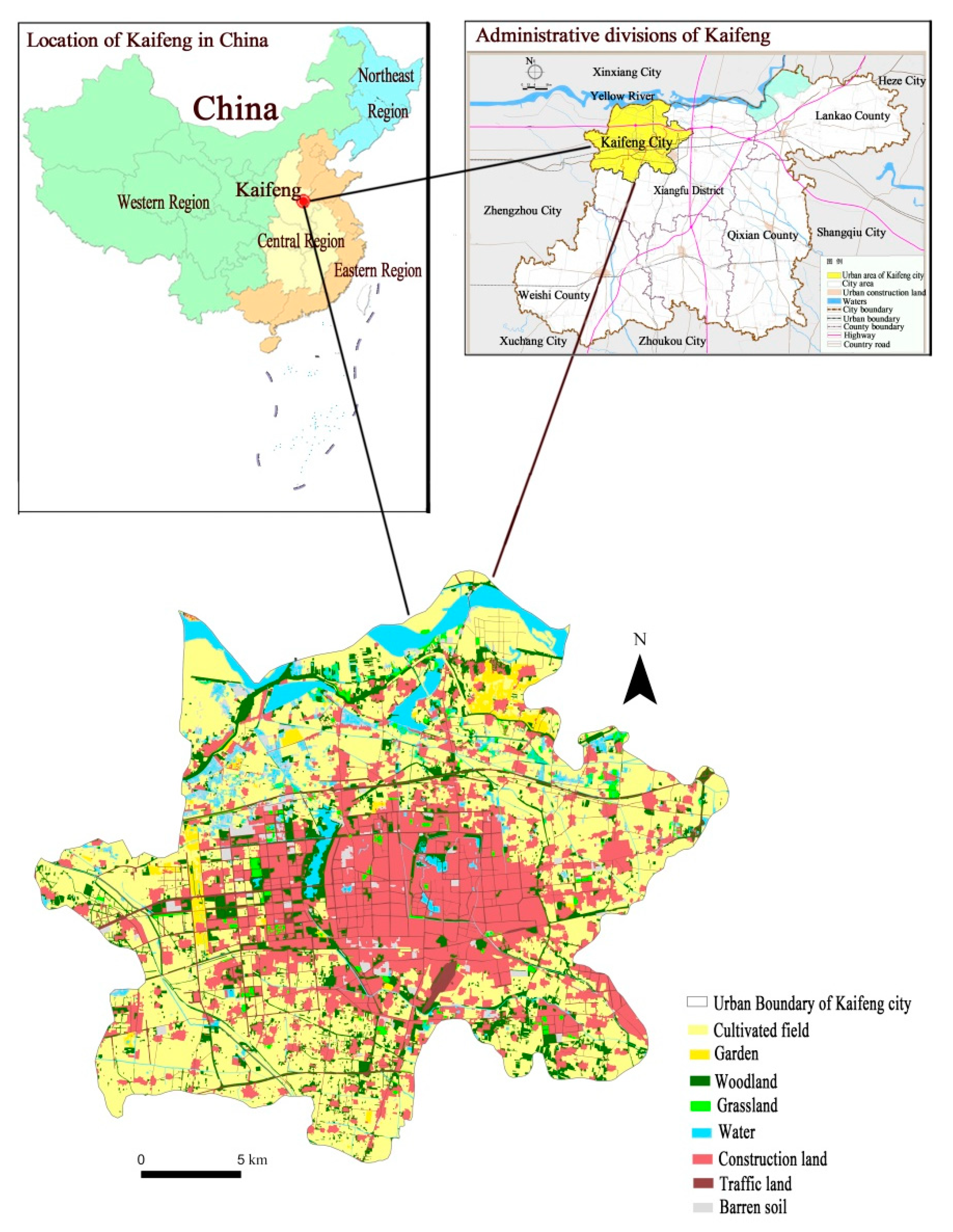
Kaifeng (113°52′15″ E—115°15′42″ E, 34°11′45″ N—35°01′20″ N) is located in the North China Plain, close to the Yellow River. It is one of the first batch of national historical and cultural cities announced by the State Council of China, and one of the famous eight ancient capitals in China. The study area in this paper is the urban area of Kaifeng City, with a total extent of about 548 km² (Figure 1). Kaifeng has a long history, and the chessboard urban layout has been preserved to this day. It is known as the “Northern Water City”. Water covers 1.70 km² of the old city, accounting for roughly a quarter of its area. The connected water system provides unique inherent advantages for the construction of a GI network. Kaifeng is an important case study for the ecological protection of the Yellow River. Optimizing the layout of GI in cities along the Yellow River is of great significance to the protection and high-quality development of the Yellow River.

The data sources of land-use map is the basis for GI network mapping [11]. Considering the small research scope and high precision requirements, we choose Gaofen-1 remote sensing satellite imagery (2017.5.12) as the data source. Then, we made manual visual interpretations using ArcGIS 10.3 to create a current land use map of the study area with a resolution of 2.5 m according to the ground features (Figure 1). The spatial classification and main interpretation signs of visual interpretation are shown in Appendix A 

Table A1. The spatial classification and main interpretation signs of visual interpretation.

First Class Name	Second Class Name	Description	Signs of Image Interpretation
Cultivated field	Paddy field	Refers to cultivated land that has water source guarantees and irrigation facilities that can be irrigated normally in normal years for the cultivation of aquatic crops such as rice and lotus roots, including cultivated land where rice and dry land crops are rotated.	Grayish purple or grayish green, regular flakes or blocks, single tone, flat surface.
	Dry land	Refers to cultivated land without water sources and facilities for irrigation and relying on natural precipitation to grow crops; cultivated land with water sources and irrigation facilities that can be irrigated normally under dry crops in normal years; Cultivated land mainly for growing vegetables, fallow land and rotation land for normal crop rotation.	Light grayish green or light earthy brown, irregular flakes, strips or blocks, single tone, flat surface.
	Facility agricultural land	Refers to the land used directly for commercial breeding of livestock and poultry houses, factory crop cultivation or aquaculture production facilities and their corresponding ancillary land, and land for agricultural facilities such as drying yards other than rural homesteads.	The image shows white or yellow regular flakes or blocks with a single tone.
Garden	Orchard	Refers to the garden where fruit trees are grown.	There are neatly arranged small particles with a darker tone.
	Tea garden	Refers to the garden where tea trees are grown.	There are neatly arranged small particles, gray-green in tone, and uneven surface.
	Other fields	Refers to gardens where mulberry, rubber, cocoa, coffee, oil palm, pepper, medicinal materials and other perennial crops are grown.	There are small particles that are not neatly arranged, the color is uneven and the tones are darker, and some plots are relatively smooth and easy to be confused on flat and dry land.
Woodland	Woodland	Refers to natural woods and plantations with a canopy closure greater than 30%. Including timber forests, economic forests, shelter forests and other forest lands.	In the image, you can see the shade of the tree, the color is dark green, the tone is uneven, there are dark green irregular dots, which are flaky in the more luxuriant places, and the borders have green dots overflowing.
	Bush forest	Refers to low woodland and shrubland with a canopy density >40% and a height of less than 2 m.	The image is green, smoother than the surface of woodland, and greener than grass.
	Sparse woodland	Refers to sparse woodland with a canopy closure of 10% to 30%.	Light green irregular shape, uneven spots.
	Other woodland	Artificial forest land, ruins, and nursery without forest.	The color of the image is similar to that of natural grass, and it is light green and irregular, with uneven spots.
Grassland	High coverage grassland	Refers to natural grassland, improved grassland and mowing grass with a coverage of >50%. Such grassland generally has good water conditions, and the grass cover grows densely.	Green irregular flakes.
	Medium coverage grassland	Refers to natural grassland and improved grassland with a coverage of 20% to 50%. Such grassland generally lacks water and the grass cover is relatively sparse.	Light green irregular flakes.
	Low coverage grassland	Refers to natural grassland with a coverage of 5% to 20%. This kind of grassland lacks water, the grass is sparse, and the animal husbandry utilization conditions are poor.	Light green or gray irregular.
Water	River	Refers to the land below the water level of a river that is naturally formed or artificially excavated.	The image appears gray-green, with clear linear borders.
	Lakes	Refers to the land below the perennial water level in the naturally formed stagnant area.	The image appears gray-green or black-green, with obvious irregular flaky borders.
	Reservoirs, ponds	Refers to the land below the perennial water level in the artificially constructed water storage area.	The image appears gray-green or black-blue, with regular or irregular flakes, with clear boundaries and smooth surfaces.
	Tidal flats, wetlands	Refers to the tidal invasion zone between the high tide level and the low tide level of the coastal tide, and the land between the water level of the river and lake water during the normal period and the water level of the flood period.	White or off-white irregular flaky borders are obvious.
	Ditches	Refers to artificially constructed channels for diversion, drainage, and irrigation, including trenches, dikes, borrow pits, and embankment forests.	Black and green linear.
Construction land	Urban construction land	Refers to the land used in large, medium and small cities and built-up areas above counties and towns.	Irregular buildings are clearly visible.
	Rural settlement	Refers to rural settlements.	Irregular buildings are clearly visible.
	Industrial and mining storage land	Refers to land mainly used for industrial production and material storage sites.	Regularity.
	Other construction land	Refers to other construction land and construction sites other than the above 3 categories.	Irregularity.
Traffic land	Railroad	Refers to the land used for railway lines, light rails, stations.	The image shows a single gray-black thin line-like tone.
	Highway	Refers to land used for national roads, provincial roads, county roads and township roads.	The image appears gray or white with a single tone. Straight line or curve, passing between cities.
	Rural road	Refers to village and field roads other than highway land.	The image appears gray or black with a single tone. Not as wide as the national highway, between fields.
	Airport	Refers to the land used for the airport.	The image appears white-brown, and the aircraft is clearly visible.
Barren soil	Sand	Refers to land covered with sand and vegetation coverage below 5%, including deserts, excluding beaches in water systems.	Yellow-white honeycomb.
	Saline-alkali land	Refers to the land where the salt and alkali accumulate on the surface, the vegetation is scarce, and only the salt-tolerant plants can grow.	The image appears with white irregular flakes, with obvious graininess.
	Bare land	Refers to land with surface soil coverage and vegetation coverage below 5%.	Grayish white with high brightness, block shape, no vegetation cover on the surface, flat surface.

. Then we used high-resolution aerial photos and field surveys to correct and adjust the interpretation results.

2.2. Methods

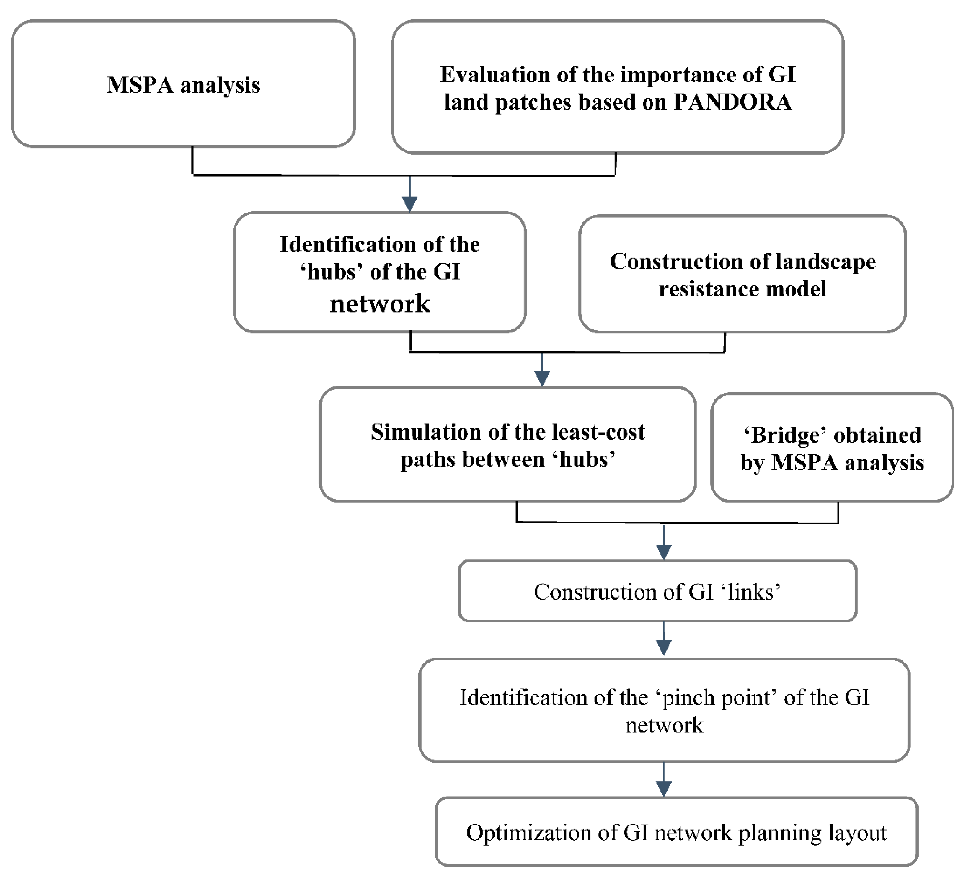
Figure 2 illustrates our methodological approach, which consists of five main steps: (1) extracting the GI elements and identifying the “core” and “bridge” landscape types based on MSPA; (2) assessing the importance of GI patches based on PANDORA; (3) identifying the GI “hubs” by analyzing both the “core” landscape type based on MSPA and the more important areas based on PANDORA; (4) simulating potential connecting corridors between ‘hubs’ based on the least-cost path method; and (5) identifying the “pinch points” of the connecting corridor through the connection model based on circuit theory.

2.2.1. MSPA Analysis

MSPA is an image processing method for identifying, measuring and classifying the spatial pattern of raster images based on the influence of variables in the mathematical morphology algorithm on the composition of the landscape pattern [31,32,33,34]. First, we converted the land-use data into a raster map with a raster size of 2.5 × 2.5 m using Guidos Tool Box software. Secondly, we brought the GI land into the foreground and assigned a value of 2, and brought other land use types into the background and assigned a value of 1. Then we converted the image to a binary raster file in TIFF format according to the assignment type. Next, we imported the raster file into Guidos Toolbox analysis software for MSPA analysis and divided the foreground into seven non-overlapping landscape types according to their shape and connectivity—Core, Bridge, Isled, Perforation, Edge, Branch, and Loop (

Table 1. The composition of landscape types in MSPA analysis and its ecological significance.

Landscape Types	Landscape Features	Ecological Significance in the GI Network
Core	A large collection of interconnected foreground pixels.	Large-scale natural patches with high connectivity which are equivalent to the hubs of the GI network.
Bridge	A collection of linear foreground pixels with high connectivity between cores.	The linear ecological land between the cores with high connectivity which is equivalent to the connecting corridor of the GI network.
Isled	A collection of foreground pixels whose area is smaller than the area threshold of the core and not interconnected with other foreground pixels.	Small natural patches that are not connected to each other which are equivalent to small patches of site in the GI network.
Perforation	Background pixels inside the core.	Unnatural patches inside the core; they can be used to assess the ecological quality of the core.
Edge	Transition pixels between foreground and background.	The transition zone between GI elements and non-GI elements.
Branch	A collection of linear foreground pixels connected to the edge of the same core at both ends.	Connecting corridors inside large natural patches.
Loop	A collection of linear foreground pixels with only one end connected to the core or the bridge.	Linear ecological land with low connectivity.

). Finally, we imported the TIFF map obtained by MSPA analysis again into the ArcGIS 10.3 software platform for geographic statistics, and further classified the area of each landscape type and its proportion in the entire landscape.

MSPA analysis needs to define four key parameters during the calculation process [35]:

(1)

Pixel size: that is, the spatial resolution of the raster image. At present, most of the research using MSPA analysis to identify ecological sources and constructing connecting corridors is applied at regional and above scales, and the spatial resolution of the land use data used is generally 30 m [36,37]. However, with the refinement of the research scale, the spatial resolution also shows a gradually increasing trend. In order to identify the smaller GI elements in the city, the spatial resolution of the land use data used in this paper is 2.5 m, that is, the pixel side length is 2.5 m.

(2)

Size parameter: It is the width of the MSPA method to perform mathematical operations such as corrosion or expansion. It is related to the width of the “edge” and “ perforation”, the minimum value of the “core” area and the maximum value of the patch area.

(3)

Structural elements: MSPA analysis uses structural elements to perform a series of logical operations on raster pixels to achieve the purpose of analyzing the structural characteristics of the landscape pattern. Structural elements refer to the basic units for calculating and processing the target landscape type map, which can be divided into two modes: eight-neighborhood and four-neighborhood. Four-neighborhood means that a certain central pixel is only considered adjacent in its basic four directions. The eight-neighborhood means that a certain central pixel is considered to be adjacent in the eight directions of its frame and the four corners of the pixel. Considering to avoid the grid connection paradox and the complex diversity of the urban landscape, this study adopts the eight-neighbor algorithm.

(4)

Edge width: It is determined by the size parameter and the pixel size. When no specific target species is set, the side length of a pixel is generally selected as the edge width by default [11]. MSPA analysis generally starts from identifying the core. The identification of the core depends on the value used to define the adjacent connection rules and the edge width [34]. The edge width affects the minimum size of the “core” and the number of pixels classified as “core”. Increasing the edge width increases the minimum size of the “core”, thereby reducing the number of pixels classified as “core”.

GI generally includes seven types of land [38]: public green land, garden land, woodland, water bodies, farmland, grassland and other green land. Kaifeng is located in the Eastern Henan Plain. Cultivated land, woodland, grassland and water bodies are important ecological resources in Kaifeng City [34,39]. Therefore, we classified cultivated land, forest, garden, grassland and water bodies as GI land, for which we set the pixel size to 1 pixel, the edge width to 1 pixel, and applied the eight-neighbor neighbor rule for MSPA analysis.

2.2.2. Evaluation of the Importance of GI Land Patches Based on PANDORA

The model based on landscape connectivity and ecosystem service assessment first proposed by Gobattoni and Pelorosso in 2011 is a mathematical model based on GIS, combined with ecological graph theory, to analyze the relationship between spatial patterns and ecological flux. Since then, Gobattoni and Pelorosso have continuously improved the model and developed an extended application PANDORA3.0 based on QGIS [4]. PANDORA3.0 uses a connectivity index (dMtot) and an ecosystem service value for each GI land type (ESV_B) to evaluate the contribution of each patch to maintaining the overall landscape connectivity.

PANDORA 3.0 compares the overall connectivity difference before and after changing a patch into an urban area, thereby calculating the contribution of each patch to maintaining the overall landscape connectivity, and determining its importance level, which is expressed by the dMtot index. The range of dMtot is between 0 and 100. The dMtot index indicates the importance of patches to the overall landscape connectivity; the larger the dMtot value, the greater the importance of the patch to the overall landscape connectivity. A patch with a dMtot index close to zero is considered to be very weakly connected to other patches in the landscape. When these patches are transformed into urbanized areas, they have less impact on the overall landscape connectivity. The dMtot index emphasizes the contribution of each patch to maintaining the overall landscape connectivity, and it is related to the bio-energy connectivity of all patches.

PANDORA3.0 can also calculate the ecosystem service value of each patch based on the ecosystem service value (ESV_B) of different land use types in biodiversity conservation proposed by Ng et al. [40] and the ES equivalent weighting factor proposed by Li et al. [41]. The ESV_B value represents the ecosystem service value of each patch based on the biodiversity present in the patch. The larger the ESV_B value, the higher the ecosystem service value of the patch.

We use PANDORA 3.0 software based on the QGIS platform, and select DEM data and soil data of the study area as model operating parameters. It uses the land use data of the study area to perform mathematical iterative calculation to simulate and calculate the dMtot values and ESV_B values of the GI land patches in the study area.

2.2.3. Identification of the ‘Hubs’ of the GI Network

We used three criteria to determine the hubs of Kaifeng City’s GI network: (1) the ‘core’ landscape determination of MSPA analysis; (2) the ecosystem service value of each land patch; and (3) the importance of a patch in maintaining connectivity of GI patches across the urban landscape. To do this, we superimposed the MSPA analysis results of GI land, the dMtot value distribution results of GI land patches, and the ESV_B value distribution results of GI land patches and analyzed them using ArcGIS 10.3 to determine the hubs of the GI network. Finally, we selected those ‘core’ landscape types that have high ecosystem service value and play an important role in maintaining overall landscape connectivity as the hubs of the GI network.

2.2.4. Construction of Landscape Resistance Model

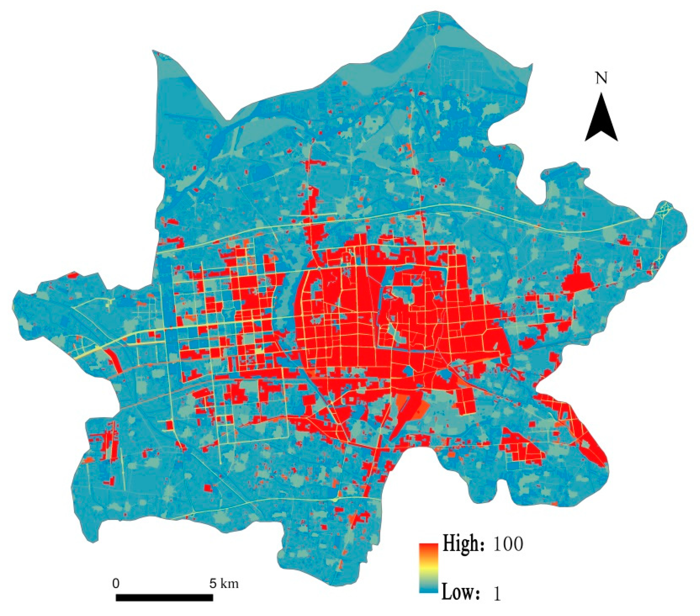
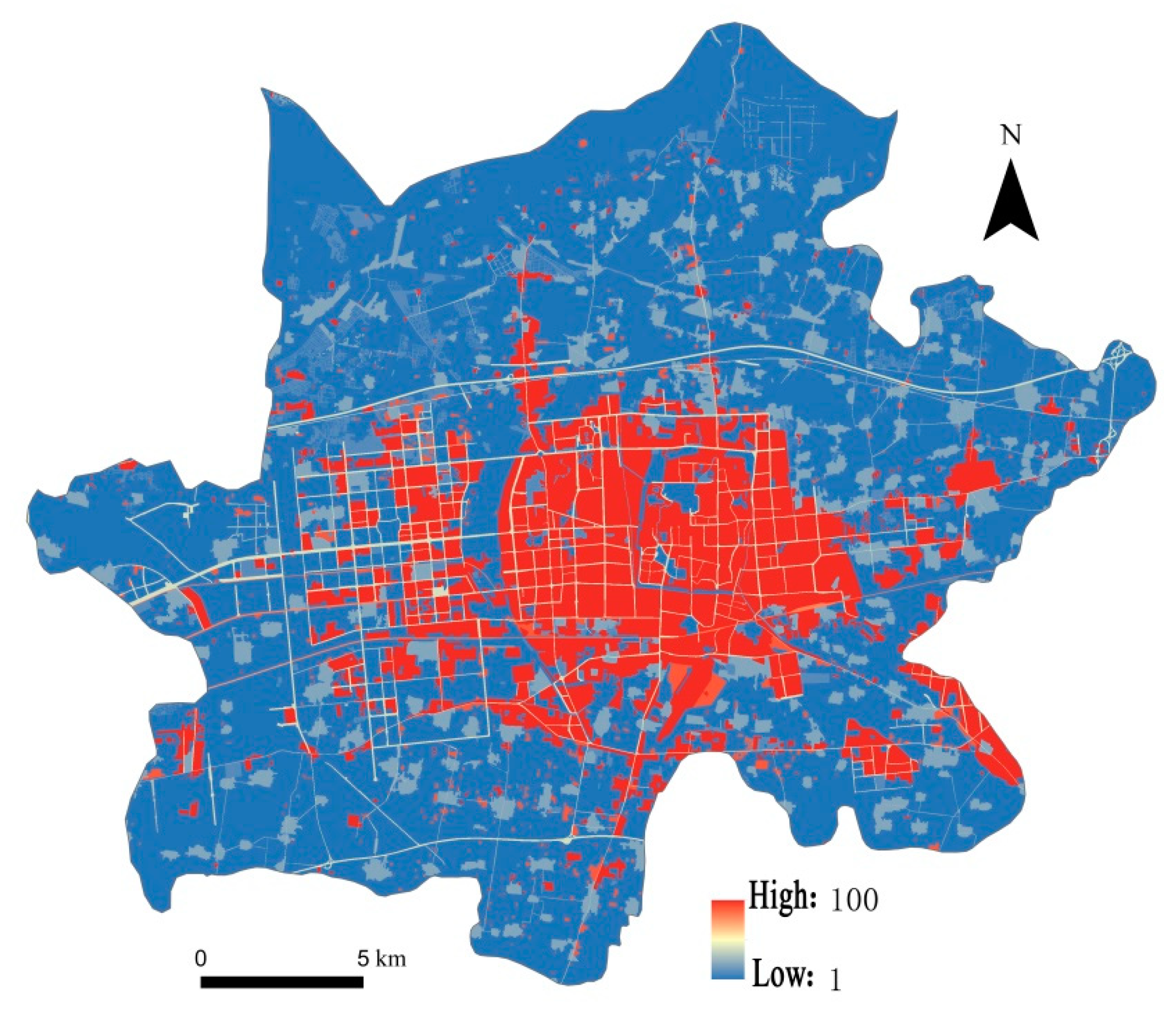
Different types of land use have different obstacles to the movement of species, that is, the value of landscape resistance is different. The landscape resistance here refers to the degree of difficulty for species to migrate between different landscape units. The higher the suitability of the patch habitat, the smaller the landscape resistance to the migration of biological species. The least-cost path method constructs a resistance surface based on the habitat suitability of the biological species based on the land use type. Through literature research, we found that there is no uniform standard for the setting of landscape resistance [37,42,43], however, the principle of resistance value setting is to set a relative value according to the ability of plaque to prevent biological movement. Therefore, this study refers to the results of previous research and sets the resistance values of different landscape types between 1 and 100 according to the degree to which they hinder energy flow and material exchange [37,42,43,44]. Forest land has the lowest resistance of 1. The resistance of urban construction land is the highest, with a resistance value of 100 (

Table 2. Resistance values of different land types.

Land Types	Woodland	Cultivated Field	Water	Rural Settlement	Urban Construction Land	Railway/Highway	Other Roads
Resistance (1–100)	1	10	15	20	100	80	40

). The distribution of landscape resistance values for different types of land is shown in Figure 3.

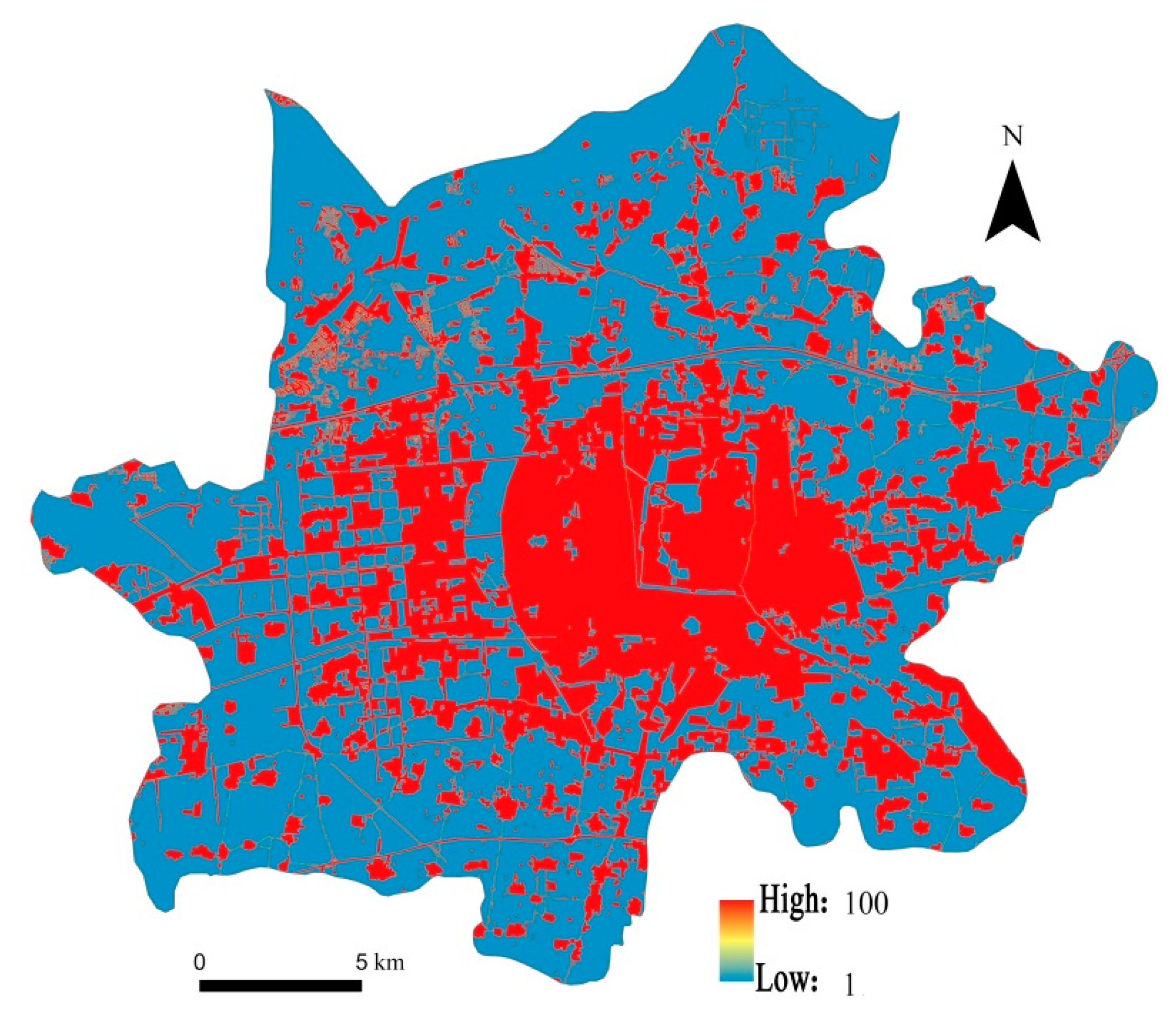
According to the resistance of different landscape types to species movement obtained by MSPA analysis, different resistance values are assigned to them [37,42,43,44] (

Table 3. The resistance values of MSPA landscape types.

Landscape Type	Core	Bridge	Islet	Performation	Edge	Loop	Branch	Background
Resistance (1–100)	1	10	15	80	30	30	60	100

). Based on the MSPA analysis, the resistance value distribution maps of different landscape types are obtained (Figure 4).

Each landscape resistance assignment method takes different factors into consideration, but both reflect the degree of hindrance of different landscape types to species movements. To integrate the resistance values, we superimposed them, giving each 50% of the weight, thereby creating a comprehensive resistance value distribution map of the study area (Figure 5).

2.2.5. Simulation of the Least-Cost Paths between ‘Hubs’

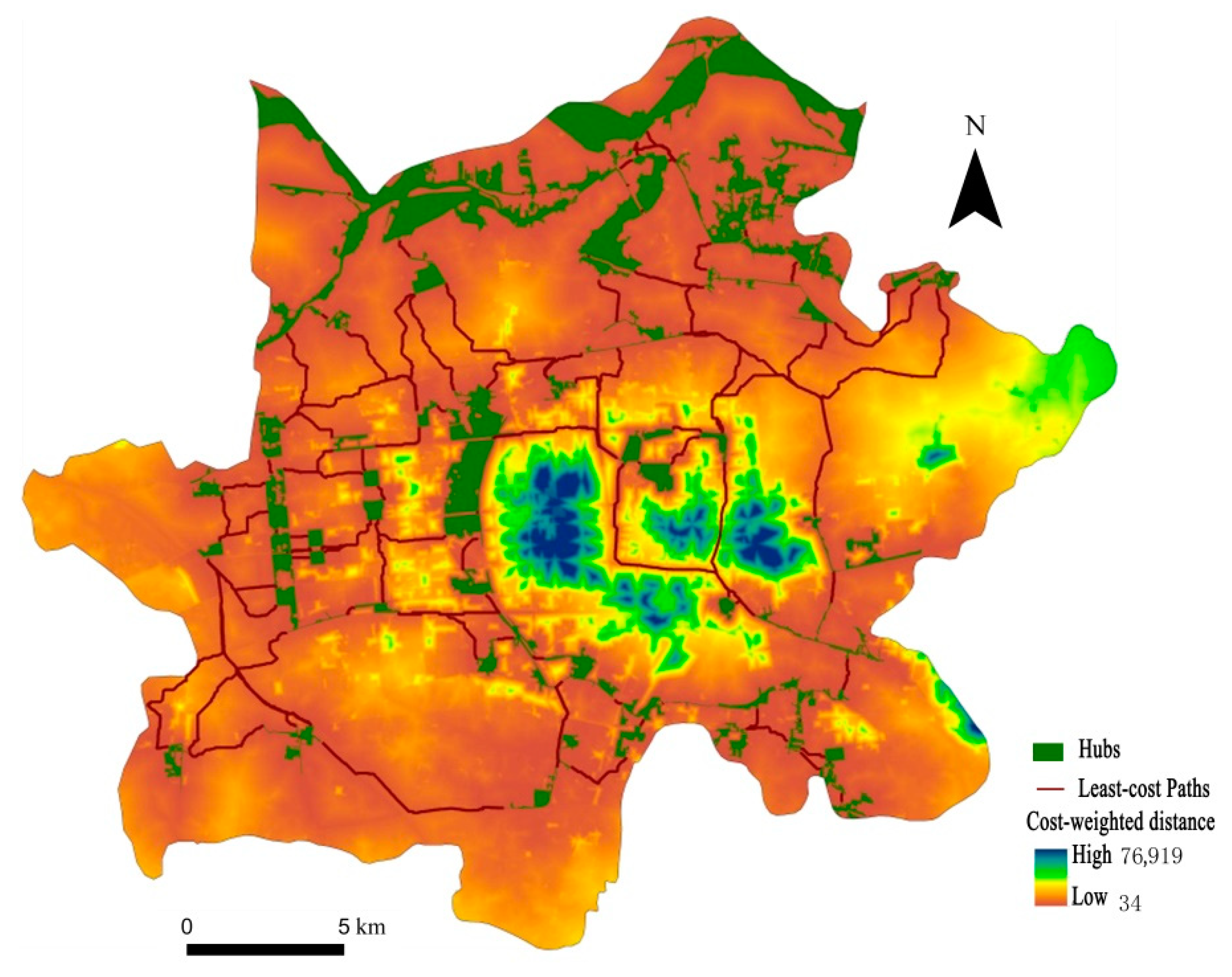
Again using ArcGIS 10.3, we used Linkage Mapper 2.0 to simulate the least-cost paths between the ‘hubs’ of the GI network. This method creates a cost-weighted distance (CWD) surface by calculating the CWD of each pixel from the nearest ‘hub’. By calculating the minimum cost-weighted distance, this method simulates the potential connecting corridors between the ‘hubs’.

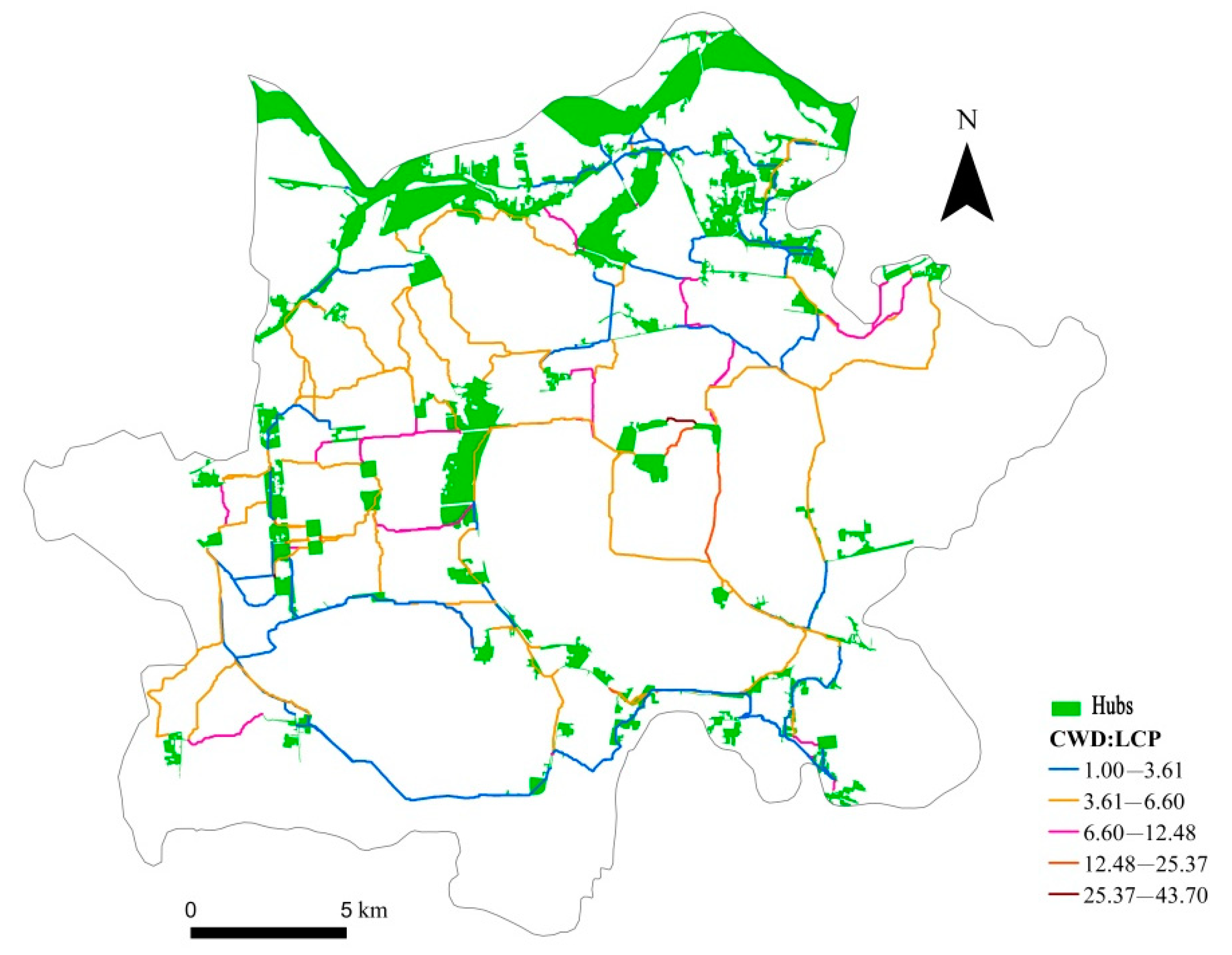
The ratio of the CWD to the least-cost path length (LCPL) can reflect the characteristics of the least-cost path. The larger the ratio, the greater the relative resistance of the path.

2.2.6. Identification of the ‘Pinch Point’ of the GI Network

We used the software Circuitscape to identify the ‘pinch points’ of the connecting corridors, analyze the importance of the connecting corridors, and determine the key areas that need priority protection in the green infrastructure network. This is an important part of optimizing the network structure of green infrastructure. ‘Pinch point’ refers to an area with a higher current density, which is an irreplaceable area that organisms prefer to choose or must pass through in the process of migration. Once the land use types in these areas change, it will seriously affect the survival of species.

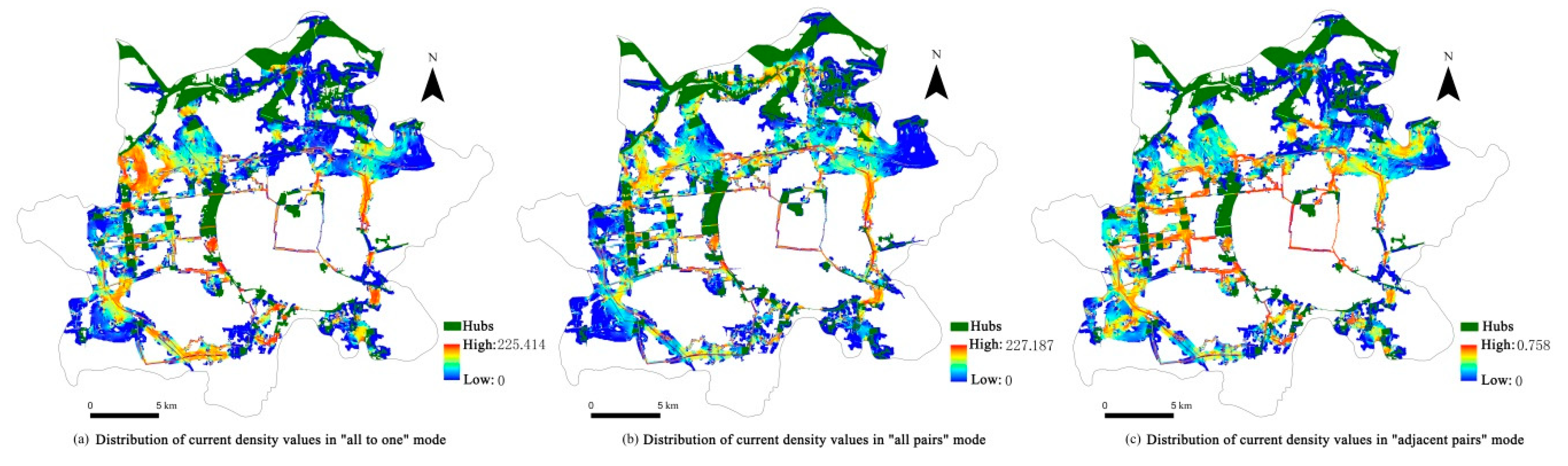
Again in ArcGIS 10.3, we used the Pinchpoint Mapper tool to calculate the current density of each corridor and distinguished the importance of the connecting corridors and the key ‘pinch point’ areas in a corridor by limiting the current to the best path. Pinchpoint Mapper has three modes to simulate the current density of the corridor, namely the ‘adjacent pair model’, the ‘all to one model’ and the ‘all pairs model’. The ‘adjacent pair model’ calculates the current intensity in the connecting corridor between two adjacent nodes. For every two adjacent nodes, one node will be arbitrarily connected to a 1A current source, and the other will be connected to the ground; then iterative calculations are performed to simulate the current intensity between two adjacent nodes. The ‘all pairs model’ calculates the current intensity of the connecting corridor between all nodes. For each pair of nodes, one node will be arbitrarily connected to a 1A current source, and the other will be connected to the ground, and then iterative calculations are performed to simulate the current intensity between all nodes. This mode requires a lot of calculations and runs slower. The ‘all to one model’ does not calculate the current intensity between all pairs of nodes; instead it connects one node to the ground, connects all the remaining nodes to a 1A current source, and then repeats the process for each node.

We used a width of 5000 m for the connecting corridor and mapped the current density distributions obtained by the three calculation modes. In order to clarify the influence of the connecting corridor width on the current density value distribution, we also set connecting corridor widths to 500, 1000, 2000, and 5000 m, again carrying out the analysis with all three Pinchpoint Mapper modes.

3. Results

3.1. MSPA Analysis

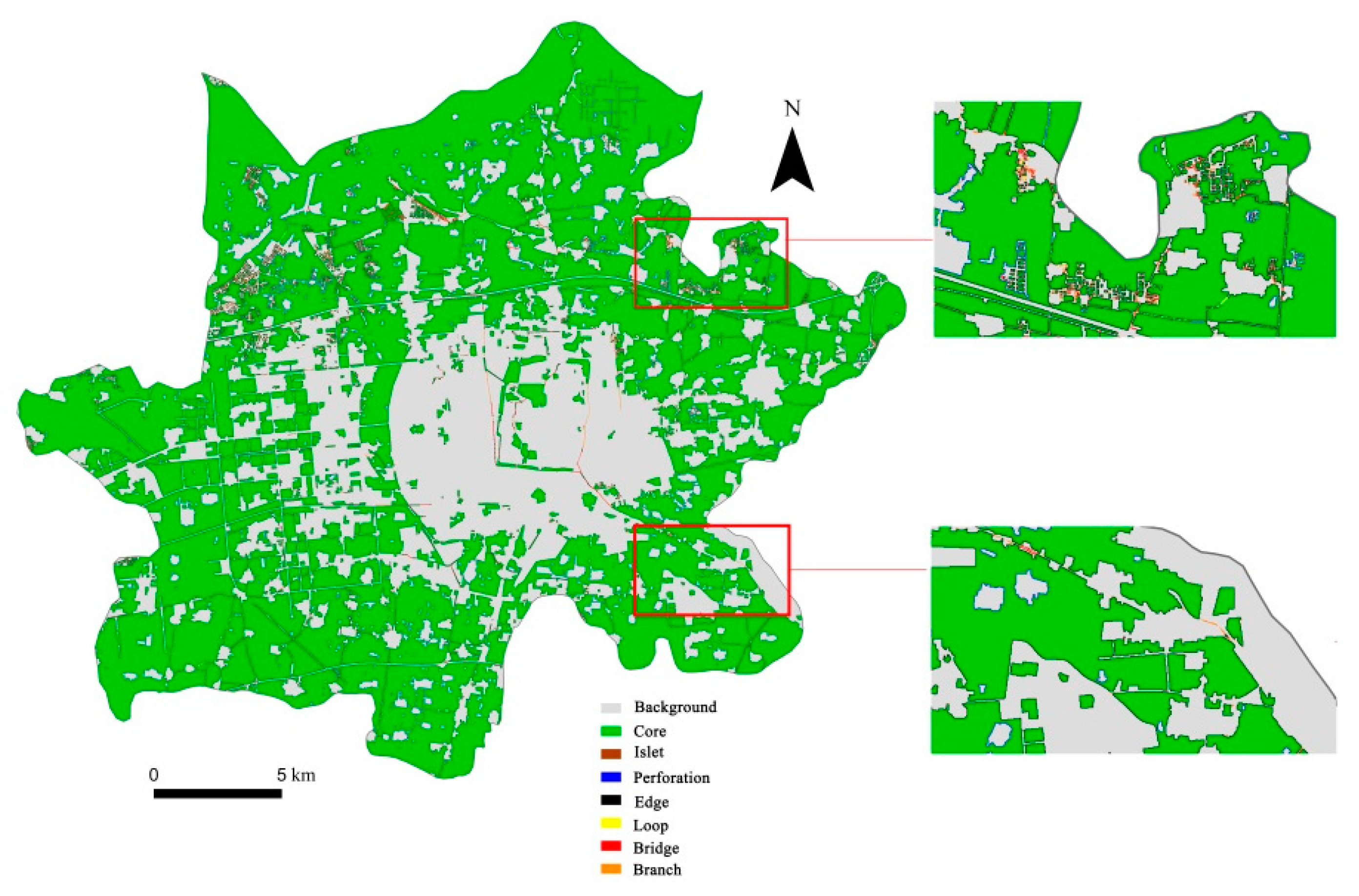
MSPA analysis found that 64.61% of the land in the study area can be used as GI land, of which 59.18% has good connectivity. More than half of the land in the study area was identified as the ‘core’. However, the main type of land that constitutes the core is cultivated land, which is mainly distributed in the suburbs around the study area, and its ability to provision ecosystem services is relatively modest. The ‘bridges’ form the main structure of the GI corridor and are thus scattered around the study area. They are always adjacent to the core, but have not yet formed a coherent GI network (Figure 6,

Table 4. Area and proportion of MSPA landscape types in Kaifeng City.

Landscape Type	Core	Islet	Perforation	Edge	Loop	Bridge	Branch	Background	Total
Area/km2	324.39	0.11	5.31	21.26	0.48	1.32	1.26	193.96	548.12
Proportion/%	59.18	0.02	0.97	3.88	0.09	0.24	0.23	35.39	100.00

).

3.2. Evaluation of the Importance of GI Land Patches

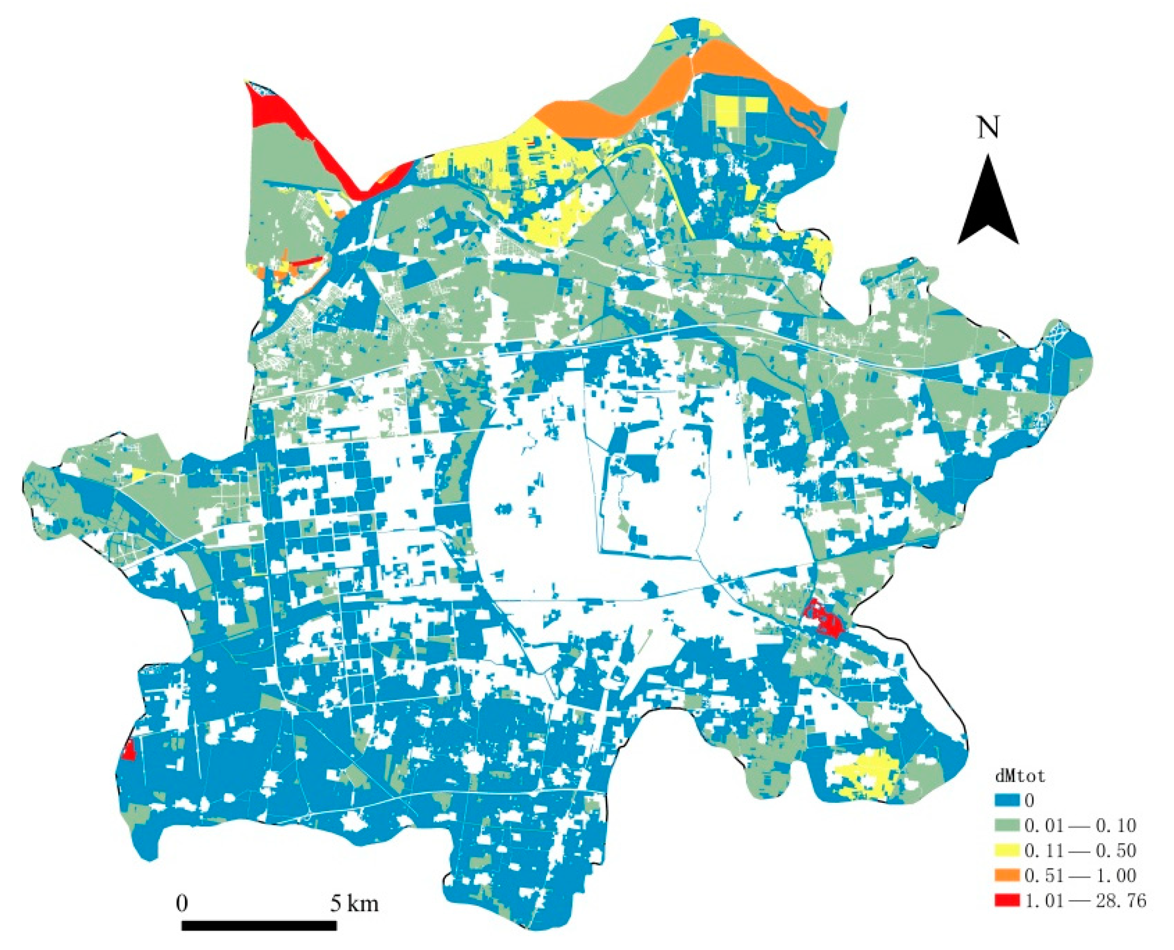
The dMtot value of the GI land patches in the study area ranged between 0 and 28.76 (Figure 7,

Table 5. Distribution area and proportion of dMtot value of GI patches in the study area.

dMtot	Area (km2)	Percentage of Total GI Area (%)	Land Cover Type	Area (km2)	Percentage of Total Area of dMtot Value Type(%)
0	189.18	53.91	cultivated land	113.35	59.92
			woodland	54.79	28.96
			garden	10.42	5.51
			water	7.05	3.73
			grassland	3.57	1.88
0.01–0.10	135.05	38.49	cultivated land	107.10	79.30
			water	20.22	14.97
			grassland	4.00	2.96
			woodland	3.51	2.60
			garden	0.22	0.17
0.11–0.50	14.08	4.01	cultivated land	13.4	95.17
			grassland	0.42	2.98
			woodland	0.26	1.85
0.51–1.00	8.57	2.44	water	7.36	85.88
			cultivated land	0.42	4.90
			grassland	0.74	8.63
			woodland	0.05	0.59
1.01–28.76	4.02	1.15	water	3.05	75.87
			cultivated land	0.95	23.63
			woodland	0.02	0.50
Total	350.90	100		350.90

), which means that the patches were unevenly distributed. 53.91% of the total GI area had a dMtot value of 0, of which 59.92% is cultivated land. This indicates that these patches have poor connectivity with other patches, and the conversion of these patches in the process of urban development has little impact on the overall landscape connectivity. The aggregated extent of GI patches with a dMtot value greater than 0.1 is only 26.67 km², accounting for 7.6% of the total GI, indicating a limited extent of GI patches with high connectivity in the study area and that the overall connectivity is low. GI patches with high dMtot values are mainly water bodies. 82.68% of GI patches with a dMtot value great than 0.5 are water bodies, mainly ones distributed in the northern portion of the study area along the Yellow River.

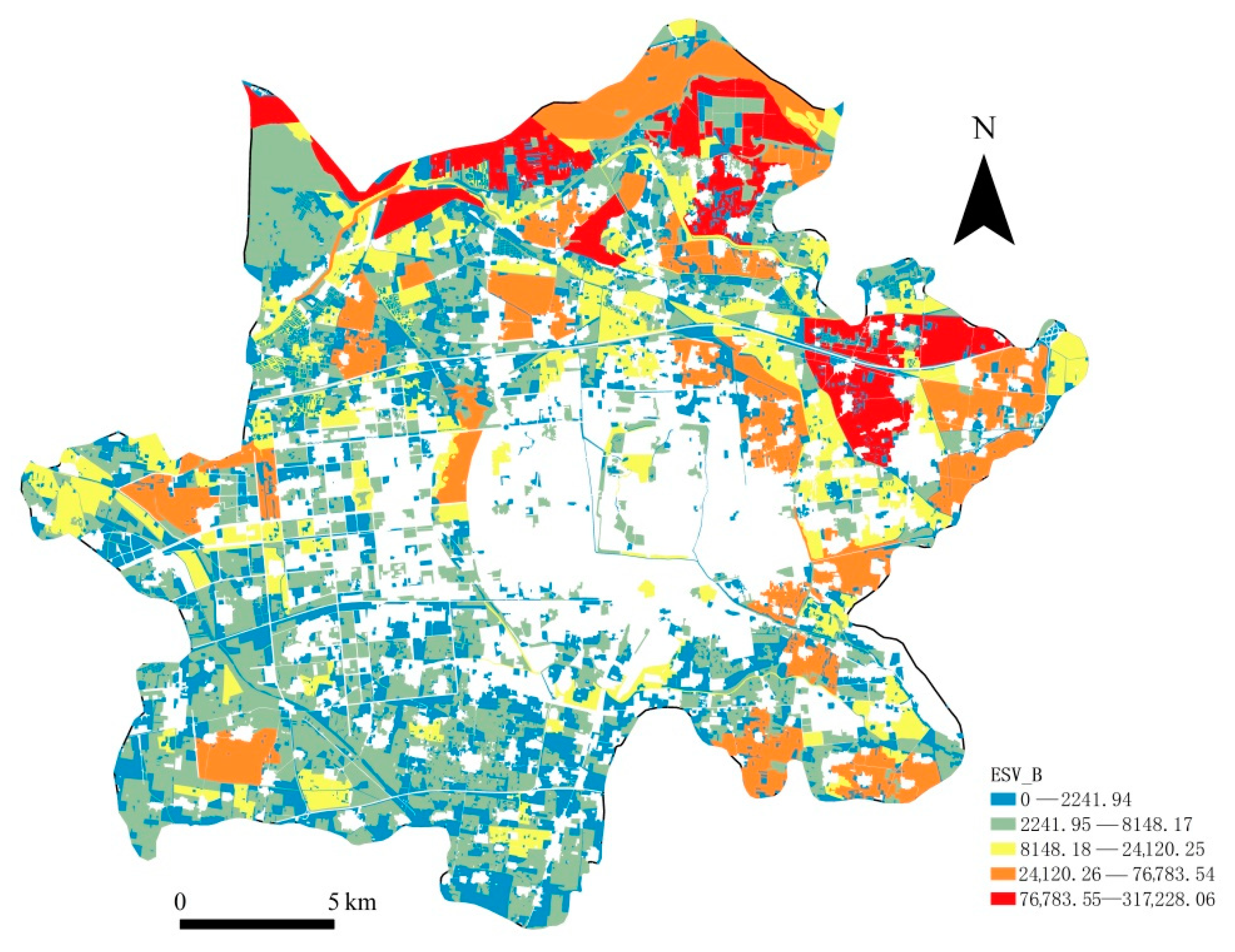
The ESV_B value of the GI patches in the study area ranged from 0 to 317,228.06 (Figure 8,

Table 6. Distribution area and proportion of ESV_B value of GI patches in the study area.

ESV_B	Area (km2)	Percentage of Total GI Area (%)	Land Cover Type	Area (km2)	Percentage of Total Area of ESV_B Value Type (%)
0–2241.94	90.52	25.81	cultivated land	53.29	58.87
			woodland	23.92	26.43
			water	10.29	11.37
			grassland	2.03	2.24
			garden	0.99	1.09
2241.95–8148.17	105.49	30.07	cultivated land	70.68	67.00
			woodland	22.49	21.32
			grassland	5.24	4.96
			water	4.70	4.46
			garden	2.38	2.26
8148.18–24,120.25	58.52	16.69	cultivated land	41.43	70.79
			woodland	9.32	15.92
			water	3.31	5.66
			garden	3.00	5.13
			grassland	1.46	2.50
24,120.26–76,783.54	56.35	16.02	cultivated land	50.11	88.93
			water	2.78	4.93
			woodland	1.97	3.49
			garden	1.49	2.65
76,783.55–317,228.06	40.02	11.41	cultivated land	22.12	55.27
			water	15.12	37.78
			garden	2.78	6.95
Total	350.90	100		350.90

). Patches with high ESV_B values are mainly distributed in the northern part of the study area, and their types of land use include cultivated land, water bodies and garden plots.

We found that most quantiles of ESV_B values in the study area are relatively scattered. The exceptions are the highest ESV_B values, which are mainly distributed in the northern Yellow River area and in the southern suburbs. Water bodies made up a higher proportion of patches with the highest ESV_B values than did forest patches.

3.3. Construction of a GI Network

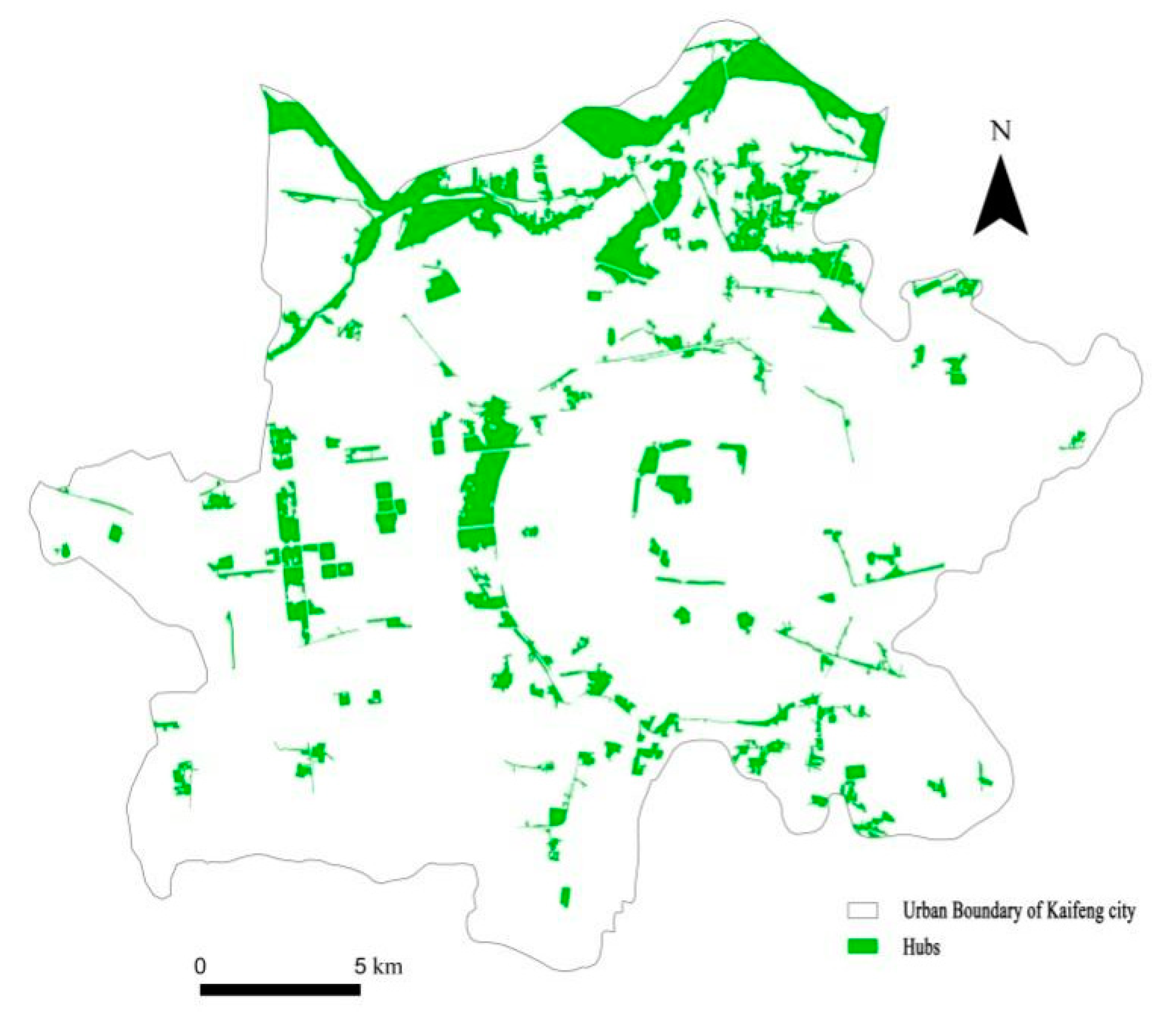
After overlay analysis, we found that 62 patches made up the ‘hubs’ of the GI network, with a total area of 53.54 km², or 9.6% of the total study area (Figure 9). Our analysis generated a total of 190 least cost paths between the ‘hubs’, with a minimum Euclidean distance of 10 m, a maximum of 7870 m, and a mean of 2101 m (Figure 10). The length of the least cost path varied greatly from 14 m to 18,372 m, with an average length of 3747 m. Minimum weighted cost distances ranged from 34 m to 76,919 m, with a mean of 16,741 m. The ratio of the cost weighted distance (CWD) to the length (LCPL) of the least-cost path can reflect the characteristics of the least-cost path. The larger the ratio, the greater the relative resistance of the path. The ratio of CWD:LCPL in the study area ranged from 1 to 43.70, with an average of 7.26 and a standard deviation of 6.60 (Figure 11). Areas with the highest CWD:LCPL ratio are located in the downtown area of Kaifeng, indicating that the relative resistance in this area is large, while the areas with the lowest ratio are located along the Yellow River to the north and in the southern suburbs.

3.4. Identification of ‘Pinch Points’

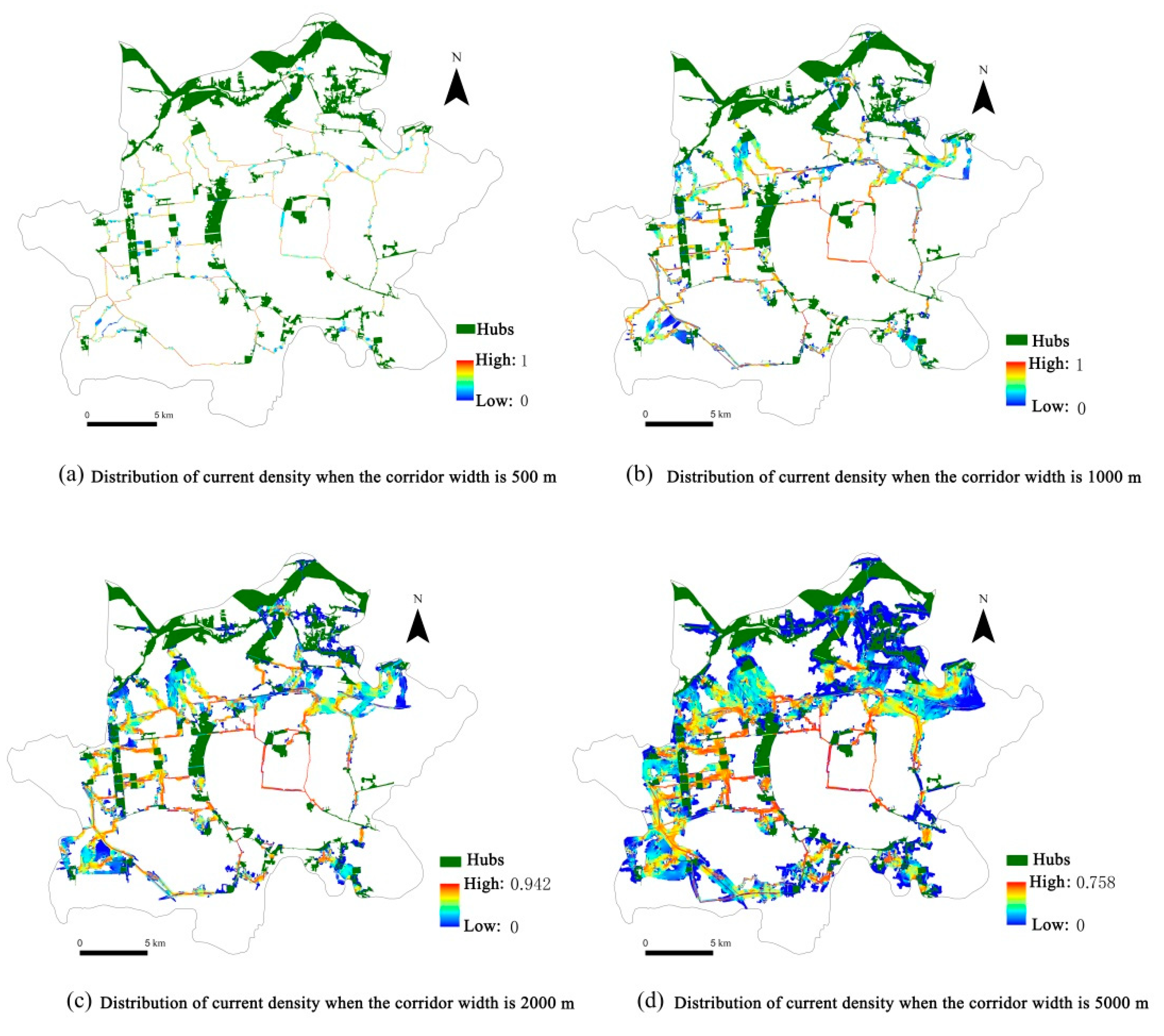
Among the three calculation modes, the adjacent pair model found the largest extent of area with high current density, primarily in the central urban area, but the highest current density value was only 0.758. The distribution patterns of high current density area obtained by ‘all pairs model’ and ‘all to one model’ simulation are the same (Figure 12). Both show that the area of high current density area is smaller than what was found by the adjacent pair model, but the highest current density values were larger. They are mainly distributed in the connecting corridors in the north-south direction of the study area. The highest current density value obtained by the ‘all to one model’ simulation is 297.38 times the highest current density value obtained by the ‘adjacent pair model’ simulation. This shows that the high current density area simulated by the “adjacent pair model” is of lower importance and has little significance in maintaining the connectivity of the entire landscape, because organisms can move between two nodes by bypassing other nodes. The ‘pinch point’ areas simulated by “all pairs model” and “all to one model” are of greater value for maintaining the connectivity of the entire landscape. In other words, these are areas where organisms must pass through or select with greater frequency while moving through the landscape. Once the habitat types of these areas change, it will seriously affect the connectivity of the entire landscape.

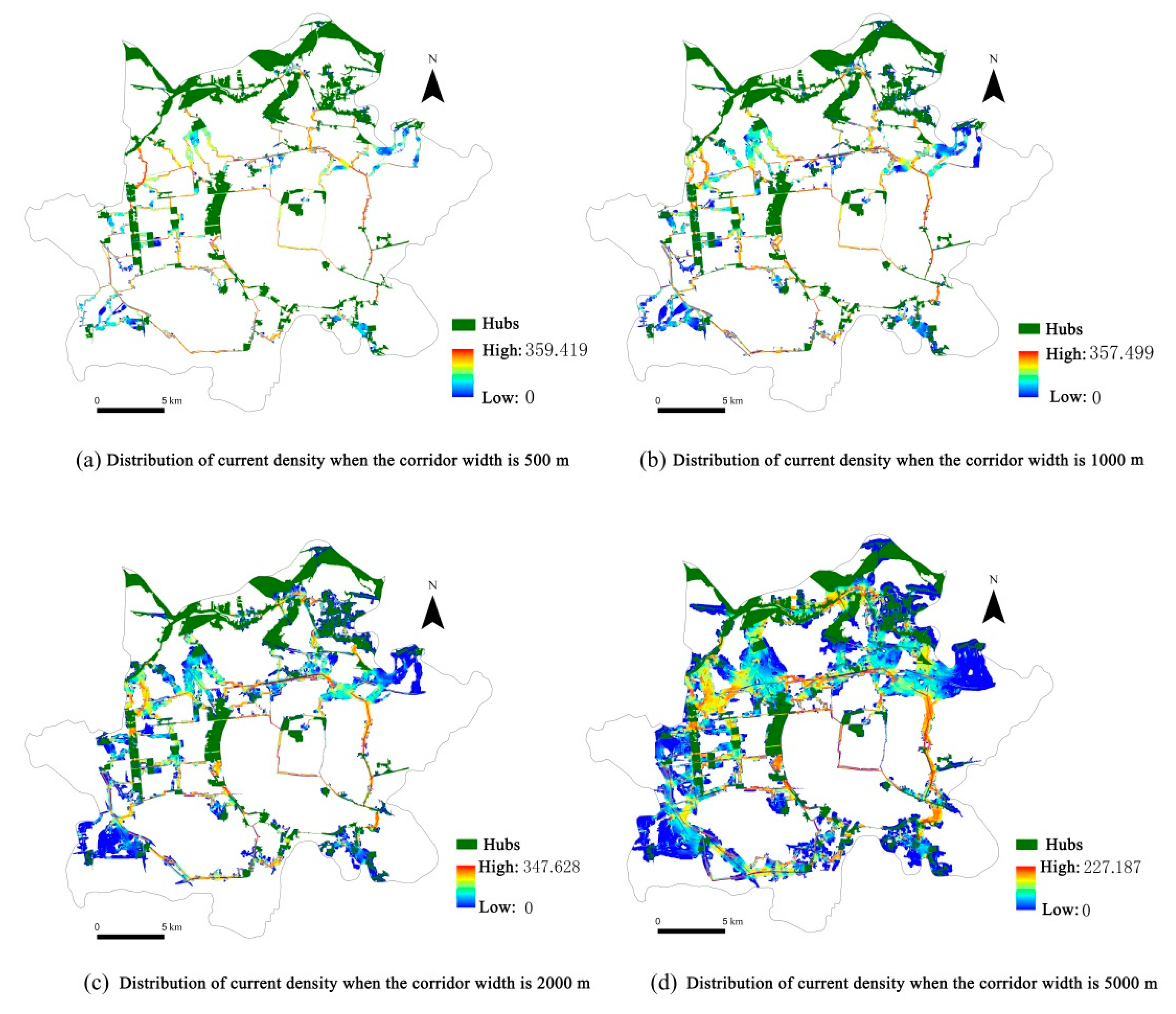
As the width of the connecting corridor increases, the maximum current density values obtained by the three calculation modes all fell, and the current density value of the ‘pinch point’ continued to decrease, but the position of the ‘pinch point’ did not change significantly. When the width of the connecting corridor in “all pairs model” is set to 500 m, the maximum current density is 359.419; and the corridor width is set to 1000 m, the maximum current density is 357.499; the corridor width is set to 2000 m, the maximum density is 347.628; and the corridor width is set to 5000 m, the maximum current density is 227.187. It can be seen that as the width of the connecting corridor increases, the maximum current density obtained by the simulation shows a gradual decrease, and the decreased amplitude gradually increases. When the width of the connecting corridor is increased from 500 to 1000 m, the maximum current density is only reduced by 1.92; when the width of the connecting corridor is increased from 1000 to 2000 m, the maximum current density is reduced by 9.871; when the width of the connecting corridor is increased from 2000 to 5000 m, the maximum current density is reduced by 120.441. In the other two modes, as the width of the connecting corridor increases, the maximum current density also changes in the same trend (Figure 13, Figure 14 and Figure 15). It can be seen that only when the width of the connecting corridor is increased to a certain extent, the maximum current density will be significantly reduced. This shows that while increasing the width of the corridor cannot significantly change the location of the ‘pinch points’ of the connecting corridors, a wider connecting corridor can provide more choices for species to move between the ‘hubs’. The larger the width of the corridor, the greater the space for this choice.

4. Discussion

4.1. MSPA Analysis

It is difficult to identify GI patches in the city that are small in area but very important to the city using 30 m resolution data. Therefore, this study used 2.5 m resolution high-definition remote sensing images to facilitate the identification of GI elements in the study area through visual inspection, and thereby improved the accuracy of the MSPA analysis. In previous studies using 30 m resolution data for MSPA analysis, the highest proportion of “core” obtained was 62.94% [14], while the proportion of “core” obtained by MSPA analysis in this study reached 91.60%. It can be seen that the higher the data resolution, the larger the proportion of “core” identified by MSPA, and the lower the proportion of the six other landscape types. Among them, the “bridge” has the largest decrease, followed by the “edge”. This finding underscores the importance of selecting an appropriate data resolution for a given research purpose.

4.2. PANDORA Analysis

Figure 4 and Figure 5 show that the distributions of the dMtot value and the ESV_B value are not the same. This shows that for patches that are more important to maintain landscape connectivity, the value of ecosystem services may not be very high, and patches with higher ecosystem services may not necessarily play an important role in maintaining overall landscape connectivity. This is consistent with the results of other related studies [4]. However, patches with both high dMtot value and high ESV_B value not only have high ecosystem service value, but also play an important role in maintaining the overall landscape connectivity. These patches play a vital role in maintaining the connectivity of GI and safeguarding its ecosystem services, and should be protected as a priority. The GI patches with both high dMtot value and high ESV_B value in the study area are mainly distributed in the northern area along the Yellow River, and the land type is mainly water. By strengthening the connectivity between water bodies, the connection between the water bodies in the central city and the northern ecological belt along the Yellow River could be improved. This shows that water bodies play an important role in maintaining the overall landscape connectivity of the study area, and the northern ecological zone along the Yellow River plays a vital role in maintaining the overall urban landscape connectivity and ecological integrity. The ecosystem service value of the northern ecological zone along the Yellow River is relatively high. This is of great significance for improving the overall urban landscape connectivity, maintaining urban ecological security and overall ecological quality.

4.3. ‘Pinch Point’ Simulation Analysis

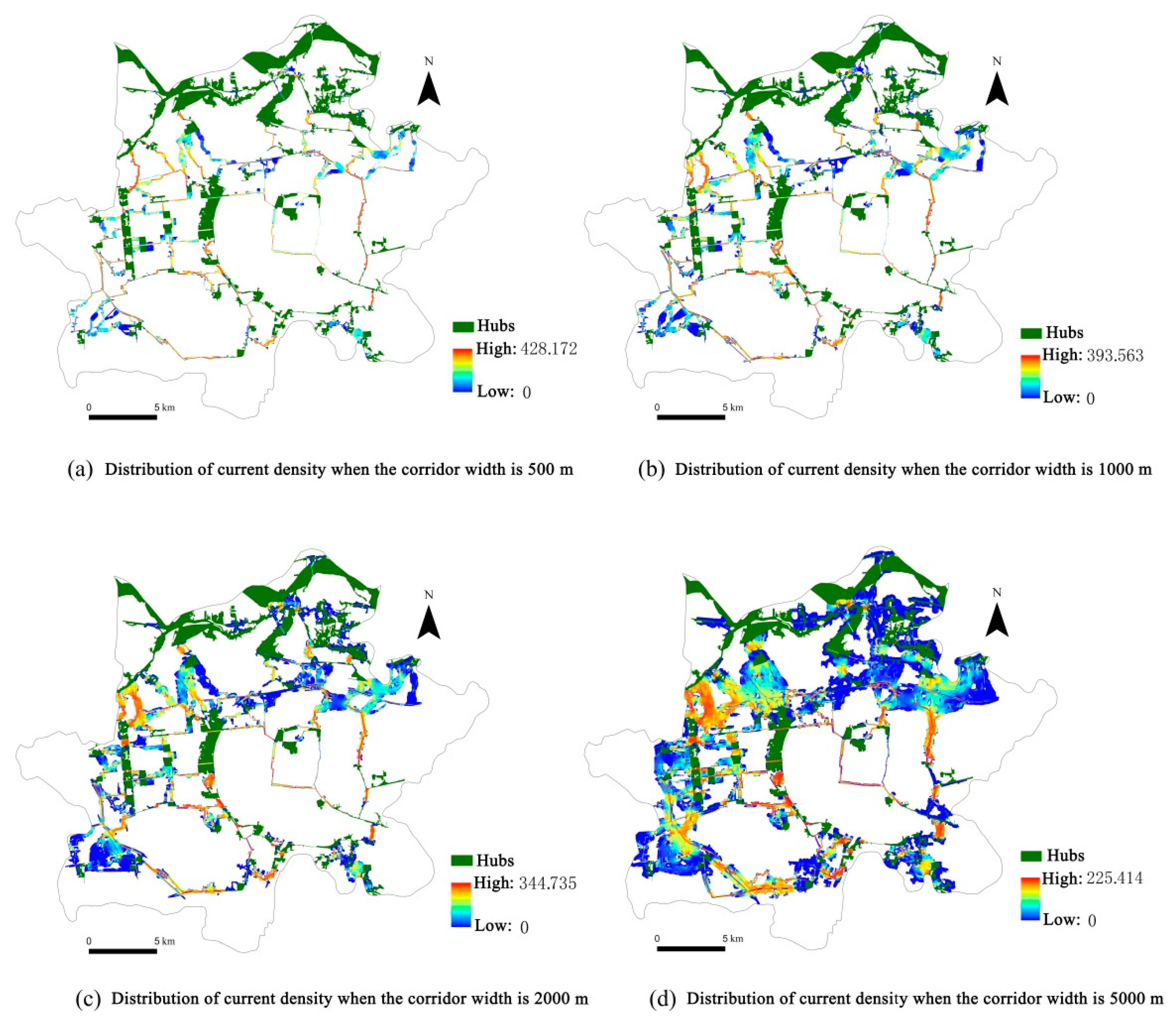
As the width of the connecting corridor increases, the difference between the maximum current density obtained by the ‘all to one model’ simulation and the maximum current density obtained by the ‘all pairs model’ simulation is becoming smaller and smaller. When the width of the connecting corridor is set to 500 m, the maximum current density simulated by the ‘all to one model’ is 68.753 times larger than the maximum current density simulated by ‘all pairs model’. When the width of the connecting corridor is set to 1000 m, the maximum current density obtained by the ‘all to one model’ simulation is 36.064 times larger than the maximum current density obtained by the ‘all pairs model’ simulation. When the width of the connecting corridor is set to 2000 m, the maximum current density obtained by the ‘all to one model’ simulation is 2.892 times smaller than the maximum current density obtained by the ‘all pairs model’ simulation. When the width of the connecting corridor is set to 5000 m, the maximum current density obtained by the ‘all to one model’ simulation is 1.773 times smaller than the maximum current density obtained by the ‘all pairs model’ simulation. It can be seen that as the width of the connecting corridor increases, the maximum current density obtained by the two modes of simulation tends to be the same. This makes intuitive sense, because when the research area is large and the calculation amount is large, the ‘all to one model’ is an effective alternative calculation model for the “all pairs model”.

As the width of the corridor increases, there are more possibilities for biological species to move between the cores, resulting in what in circuit theory would be called ‘current shunting’ and a decrease in current density. However, only when the width of the corridor is increased to more than 2000 m does the current density value change significantly. With the increase in the width of the connecting corridor, the position of the ‘pinch point’ does not change significantly, which indicates that the increase in the width of the corridor has little effect on the connectivity of the entire landscape. However, as the width of the connecting corridor increases, the irreplaceability of the ‘pinch point’ is reduced, especially when the width of the connecting corridor is large, the current density value decreases significantly. This shows that although increasing the corridor width cannot significantly improve the overall connectivity of the landscape, it can effectively improve the ecological security of the landscape. It is consistent with the results of other related studies [45].

It can be seen that the current density value obtained by the ‘adjacent pair model’ simulation is relatively small, and the ‘pinch point’ obtained by the simulation of this model is of lower importance and has little effect on maintaining the connectivity of the entire landscape. However, increasing the width of the connecting corridor can still reduce the maximum current density and improve the ecological connectivity between the two nodes.

5. Conclusions

Using Kaifeng City as a case study, we were able to objectively identify key pinch points in a green infrastructure network by using a framework that incorporates three distinct models: MSPA, PANDORA, and a connection model based on circuit theory. Our study found that patches with both high ESV_B value and high dMtot value are mainly distributed in the area along the Yellow River in the north of Kaifeng City, and the land type is mainly water. This shows that prioritizing the protection of the northern ecological zone along the Yellow River and improving the connection between the central urban area and the northern ecological zone along the Yellow River are of great significance for improving the overall landscape connectivity, maintaining urban ecological security and overall ecological quality. We identified 62 ‘hubs’ with an area of 53.54 km², accounting for 9.6% of the total area of the study area. The land use type of “hubs” is mainly water, and there are few large and high-quality forest land patches. The landscape heterogeneity of “hubs” is low. Our model produced a total of 190 hypothetical connecting corridors between the ‘hubs’ and ‘pinch points’. Connecting corridors mainly ran in the north-south direction of the study area. Increasing the width of the connecting corridors did not significantly change the position of the ‘pinch points’. It did, however, reduce their irreplaceability, especially for simulations where the width of the connecting corridor was greater than 2000 m, at which point the current density value decreased significantly. This shows that although increasing the corridor width cannot significantly improve the overall connectivity of the landscape, it can effectively improve the ecological integrity of the landscape.

The case study showed that our novel technical framework is well suited for objectively and accurately identifying green infrastructure hubs of landscape connectivity and ecosystem service value. Further, we showed the framework was capable of identifying the key ‘pinch point’ areas for improving connectivity, and verifying the influence of corridor width on connectivity. Therefore, it can provide effective technical support for urban GI planning and construction, and provide a basis for the formulation of urban sustainable development strategies.

References

- Saura, S.; Pascual-Hortal, L. A new habitat availability index to integrate connectivity in landscape conservation planning: Comparison with existing indices and application to a case study. Landsc. Urban Plan. 2007, 83, 91–103. [Google Scholar] [CrossRef]
- Bastian, O. The role of biodiversity in supporting ecosystem services in Natura 2000 sites. Ecol. Indic. 2013, 24, 12–22. [Google Scholar] [CrossRef]
- Pelorosso, R.; Gobattoni, F.; Geri, F.; Monaco, R.; Leone, A. Evaluation of Ecosystem Services related to Bio-Energy Landscape Connectivity (BELC) for land use decision making across different planning scales. Ecol. Indic. 2016, 61, 114–129. [Google Scholar] [CrossRef]
- Pelorosso, R.; Gobattoni, F.; Geri, F.; Leone, A. PANDORA 3.0 plugin: A new biodiversity ecosystem service assessment tool for urban green infrastructure connectivity planning. Ecosyst. Serv. 2017, 26, 476–482. [Google Scholar] [CrossRef]
- Lee, V.; Zhao, Z.Y. New York Green Infrastructure Planning and Its Application to Master Planning of Sponge City in China. China Water Wastewater 2016, 15, 126–129. [Google Scholar]
- Jiang, W.W.; Sun, P. Theory research on green infrastructure: Taking green land system planning of Cixi city in Zhejiang Province as an example. J. Beijing For. Univ. Soc. Sci. 2012, 11, 54–59. [Google Scholar]
- Pei, D. Ecological conservation networks and conservation priority evaluation:Green infrastructure as a smart conservation stratege. Acta Sci. Nat. Univ. Pekin. 2012, 48, 848–854. [Google Scholar]
- Williamson, K.B. Growing with Green Infrastructure; Heritage Conservancy: Doylestown, PA, USA, 2003. [Google Scholar]
- Pei, D. Review of Green Infrastructure Planning Methods. City Plan. Rev. 2012, 36, 84–90. [Google Scholar]
- Li, K.R. Green Infrastructure: Concept, Theory and Practice. Chin. Landsc. Archit. 2009, 25, 88–90. [Google Scholar]
- Wickham, J.; Riitters, K.; Vogt, P. A national assessment of green infrastructure and change for the conterminous United States using morphological image processing. Landsc. Urban Plan. 2010, 94, 186–195. [Google Scholar] [CrossRef]
- Benedict, M.; Macmahon, E.T. Green Infrastructure: Smart Conservation for the 21st Century. Renew. Resour. J. 2002, 20, 12–17. [Google Scholar]
- Ahern, J. Green Infrastructure for Cities: The Spatial Dimension; IWA Publications: London, UK, 2007; pp. 267–283. [Google Scholar]
- Shi, X.M.; Qin, M.Z. Research on the Optimization of Regional Green Infrastructure Network. Sustainability 2018, 10, 4649. [Google Scholar] [CrossRef] [Green Version]
- Wei, J.; Qian, J.; Tao, Y.; Hu, F.; Ou, W. Evaluating Spatial Priority of Urban Green Infrastructure for Urban Sustainability in Areas of Rapid Urbanization: A Case Study of Pukou in China. Sustainability 2018, 10, 327. [Google Scholar] [CrossRef] [Green Version]
- Weber, T.; Sloan, A.; Wolf, J. Maryland’s Green Infrastructure Assessment: Development of a comprehensive approach to land conservation. Landsc. Urban Plan. 2006, 77, 94–110. [Google Scholar] [CrossRef]
- Meerow, S.; Newell, J.P. Spatial planning for multifunctional green infrastructure: Growing resilience in Detroit. Landsc. Urban Plan. 2017, 159, 62–75. [Google Scholar] [CrossRef]
- Taylor, L.; Hochuli, D.F. Creating better cities: How biodiversity and ecosystem functioning enhance urban residents’ wellbeing. Urban Ecosyst. 2014, 18, 747–762. [Google Scholar] [CrossRef]
- Pan, H.; Deal, B.; Destouni, G.; Zhang, Y.; Kalantari, Z. Sociohydrology modeling for complex urban environments in support of integrated land and water resource management practices. Land Degrad. Dev. 2018, 29, 3639–3652. [Google Scholar] [CrossRef] [Green Version]
- Wu, Y.X.; Liu, X.G.; Wu, B.; Yuan, X.J. Regional green infrastructure space pattern identification based on urban air conditioning. Landsc. Archit. 2018, 29, 33–36. [Google Scholar]
- Cannas, I. Green Infrastructure and Ecological Corridors: A Regional Study Concerning Sardinia. Sustainability 2018, 10, 1265. [Google Scholar] [CrossRef] [Green Version]
- Gobattoni, F.; Pelorosso, R.; Lauro, G.; Leone, A.; Monaco, R. A procedure for mathematical analysis of landscape evolution and equilibrium scenarios assessment. Landsc. Urban Plan. 2011, 103, 289–302. [Google Scholar] [CrossRef]
- Gobattoni, F.; Groppi, M.; Monaco, R.; Pelorosso, R. New Developments and Results for Mathematical Models in Environment Evaluations. Acta Appl. Math. 2014, 132, 321–331. [Google Scholar] [CrossRef]
- Gobattoni, F.; Lauro, G.; Monaco, R.; Pelorosso, R. Mathematical Models in Landscape Ecology: Stability Analysis and Numerical Tests. Acta Appl. Math. 2012, 125, 173–192. [Google Scholar] [CrossRef] [Green Version]
- McRae, B.H.; Dickson, B.G.; Keitt, T.H.; Shah, V.B. Using circuit theory to model connectivity in ecology, evolution, and conservation. Ecology 2008, 89, 2712–2724. [Google Scholar] [CrossRef] [PubMed]
- Mcrae, B.H. Isolation by Resistance. Evolution 2006, 60, 1551–1561. [Google Scholar] [CrossRef] [PubMed]
- Hansen, R.; Pauleit, S. From Multifunctionality to Multiple Ecosystem Services? A Conceptual Framework for Multifunctionality in Green Infrastructure Planning for Urban Areas. Ambio 2014, 43, 516–529. [Google Scholar] [CrossRef] [PubMed] [Green Version]
- Mcrae, B.H.; Beier, P. Circuit theory predicts gene flow in plant and animal populations. Proc. Natl. Acad. Sci. USA 2007, 104, 19885–19890. [Google Scholar] [CrossRef] [PubMed] [Green Version]
- Adriaensen, F.; Chardon, J.P.; De Blust, G.; Swinnen, E.; Villalba, S.; Gulinck, H.; Matthysen, E. The application of ‘least-cost’ modelling as a functional landscape model. Landsc. Urban Plan. 2003, 64, 233–247. [Google Scholar] [CrossRef]
- Urban, D.; Keitt, T. Landscape Connectivity: A Graph-Theoretic Perspective. Ecology 2001, 82, 1205–1218. [Google Scholar] [CrossRef]
- Vogt, P.; Ferrari, J.R.; Lookingbill, T.R.; Gardner, R.H.; Riitters, K.H.; Ostapowicz, K. Mapping functional connectivity. Ecol. Indic. 2009, 9, 64–71. [Google Scholar] [CrossRef]
- Vogt, P.; Riitters, K.H.; Iwanowski, M.; Estreguil, C.; Kozak, J.; Soille, P. Mapping landscape corridors. Ecol. Indic. 2007, 7, 481–488. [Google Scholar] [CrossRef]
- Saura, S.; Vogt, P.; Velázquez, J.; Hernando, A.; Tejera, R. Key structural forest connectors can be identified by combining landscape spatial pattern and network analyses. For. Ecol. Manag. 2011, 262, 150–160. [Google Scholar] [CrossRef]
- Soille, P.; Vogt, P. Morphological Segmentation of Binary Patterns. Pattern Recognit. Lett. 2009, 30, 456–459. [Google Scholar] [CrossRef]
- Cao, Y.K.; Fu, M.C.; Xie, M.M.; Gao, Y.; Yao, S.Y. Landscape connectivity dynamics of urban green landscape based on morphological spatial pattern analysis (MSPA) and linear spectral mixture model (LSMM) in Shenzhen. Acta Ecol. Sin. 2015, 35, 526–536. [Google Scholar]
- Yu, Y.P.; Yin, H.W.; Kong, F.H.; Wang, J.J.; Xu, W.B. Analysis of the temporal and spatial pattern of the green infrastructure network in Nanjing, based on MSPA. Chin. J. Ecol. 2016, 35, 1608–1616. [Google Scholar]
- Xu, F.; Yin, H.W.; Kong, F.H.; Xu, J.G. Developing ecological networks based on MSPA and the least-cost path method: A case study in Bazhong western new district. Acta Ecol. Sin. 2015, 35, 6425–6434. [Google Scholar]
- Liu, W.P. Planning and Design of Green Infrastructure Based on Landscape Service; China Agricultural University: Beijing, China, 2014. [Google Scholar]
- Du, S.Q.; Yu, D.Y. Urban ecological infrastructure and its construction principles. Chin. J. Ecol. 2010, 29, 1646–1654. [Google Scholar]
- Ng, C.N.; Xie, Y.J.; Yu, X.J. Integrating landscape connectivity into the evaluation of ecosystem services for biodiversity conservation and its implications for landscape planning. Appl. Geogr. 2013, 42, 1–12. [Google Scholar] [CrossRef]
- Li, T.H.; Li, W.K.; Qian, Z.H. Variations in ecosystem service value in response to land use changes in Shenzhen. Ecol. Econ. 2010, 69, 1427–1435. [Google Scholar]
- Liu, S.; He, B. Construction of Regional Green Infrastructure Based on MSPA—Case Study on Suzhou-Wuxi-Changzhou Area. Landsc. Archit. 2017, 5, 98–104. [Google Scholar]
- Chen, Z.A.; Kuang, D.; Wei, X.J.; Zhang, L.T. Developing Ecological Networks Based on MSPA and MCR: A Case Study in YuJiang County. Resour. Environ. Yangtze Basin 2017, 8, 92–100. [Google Scholar]
- Shi, X.M.; Qin, M.Z.; Li, B.; Li, C.Y.; Song, L.L. Research on the green infrastructure network in the Zhengzhou-Kaifeng metropolitan area based on MSPA and circuit theory. J. Henan Univ. Nat. Sci. 2018, 48, 631–638. [Google Scholar]
- Song, L.L.; Qin, M.Z. Identification of Ecological Corridors and its Importance by Integrating Circuit Theory. Chin. J. Appl. Ecol. 2016, 27, 3344–3352. [Google Scholar]
Figure 1.
The research area: location and land cover types.
Figure 2.
A schematic of this paper’s green infrastructure network optimization approach and work flow.
Figure 3.
Distribution of resistance values based on land types.
Figure 4.
Distribution of resistance values based on MSPA landscape types.
Figure 5.
Distribution of comprehensive resistance values.
Figure 6.
MSPA analysis results.
Figure 7.
Distribution of dMtot value of GI patches.
Figure 8.
Distribution of ESV_B value of GI patches.
Figure 9.
Distribution of hubs.
Figure 10.
Simulation results of the least-cost paths between ‘hubs’.
Figure 11.
The distribution of the ratio of the cost-weighted distance to the length of the least-cost paths.
Figure 12.
Comparison of current density distribution of 5000 m connection width in three modes.
Figure 13.
Comparison of current density distribution of different corridor widths in “all pairs model”.
Figure 14.
Comparison of current density distribution of different corridor widths in “all to one model”.
Figure 15.
Comparison of current density distribution of different corridor widths in “adjacent pair model”.