A Software Tool for a Stochastic Life Cycle Assessment and Costing of Buildings’ Energy Efficiency Measures

Abstract

This article presents a novel software tool for the assessments of life-cycle environmental impacts and costs, which is aimed to support decision-making in the design phase of retrofit interventions in the building sector. By combining Life Cycle Costing (LCC) and Life Cycle Assessment (LCA) calculations and functionalities, this tool allows evaluating the long-term trade-offs between economic and environmental performance of investment projects in energy efficiency for buildings, while accounting for uncertainties in input parameters and economic scenarios. A major novelty of the software tool is the stochastic nature of both the LCC and LCA dimensions. The LCA is implemented with Monte-Carlo methods, while the LCC accounts for the probabilistic interdependence of macroeconomic variables over time. The software also includes advanced specific tools for parametrization and sensitivity analysis. Exemplary applications are presented in order to illustrate the novelty and the functionalities of the software tool.

1. Introduction

The transition towards a climate-neutral Europe by 2050 [1] recently confirmed by the EU Green Deal [2] is one of the most urgent challenges for the European Union (EU) in the upcoming decades. The EU has put forward several initiatives to promote and incentivize sustainable practices in an increasing number of areas during the past years, and, in the next programming periods, it is expected to continue on the path towards climate neutrality [3]. Energy efficiency improvements in the building sector are essential to achieve the long-term environmental targets of the European Union. Indeed, buildings in the EU are responsible for around 40% of final energy consumption and 36% of carbon dioxide (CO₂) emissions [4]. Thus, to reach the EU’s energy efficiency and climate objectives, the annual renovation rate of the building stock in the Member States, which today varies from 0.4 to 1.2%, will need at least to double [2]. However, this “renovation wave” will require costly investments whose returns are closely linked to highly uncertain future scenarios [5].

This article describes a novel Life Cycle Costing (LCC)/Life Cycle Assessment (LCA) software tool that is aimed to support decision-making in the design phase of retrofit interventions in the building sector. Through combined stochastic LCC and LCA functionalities, this tool allows evaluating the long-term trade-offs existing between the economic and environmental performance of investment projects in energy efficiency for buildings while accounting for uncertainties in all its input parameters and economic scenarios. By integrating the economic and environmental dimensions, the proposed methodological approach and software tool contributes to a suitable LCC and LCA assessment of these long-term projects [6].

An increasing interest is shown in the recent literature for multi-dimensional LCC, multi-dimensional LCA, and social LCA assessments of building energy retrofitting projects. However, as underlined in the review of Amini Toosi et al. [7], there are still few works that combine LCC and LCA to evaluate long-term trade-offs between the economic and environmental performance. Moreover, the role of uncertainty of life-cycle-related parameters is often overlooked, and, consequently, an appropriate sensitivity analysis is rarely performed. Moreover, concerning the available tools, sustainability assessment functionalities are separately provided by several existing software applications. However, only a few include both LCC and LCA calculations [7], and none of them explicitly considers the stochastic nature of input data and the consequent uncertainty. The IEA-EBC Annex 56 project (“Cost-Effective Energy and CO₂ Emissions Optimization in Building Renovation”), for example, developed a specific tool named A56opt-tool able to perform both LCC and LCA evaluations of building renovation measures. The tool was specifically developed to support the decision-makers for the establishment of cost-optimized targets for energy use and carbon emissions related to building renovation, also considering different co-benefits [8,9].

The LCA and LCC models presented in this paper are based on the European LCC standard EN 15459-1:2017 [10], and on the international LCA standards ISO 14040–14044 [11,12], EN 15804, and EN 15978 [13,14]. To account for the uncertainties inherent in the long-term planning horizons due to stochastic input data, Monte-Carlo (MC) methods are applied to both LCC and LCA models (uncertainty propagation) [15]. In particular, for the LCC calculations, stochastic predictions of the economic variables are generated by multivariate time-series models and used as discount factors and price escalation rates [16,17]. The resulting output of the analysis takes the form of probability distributions of economic and environmental indicators. Sensitivity Analysis (SA) can thus be performed to assess the contribution of input and scenario assumptions on these output indicators.

The explicit modelling of the stochastic nature in both LCC and LCA assessments, and the consequent sensitivity analysis, are what make this LCA/LCC software tool original compared to the available packages and constitutes the main contribution of the present paper to the existing literature. Thus, the main novelty of the work stands in the development of this tool with its different functionalities, which allow the users to apply the described uncertainty and sensitivity analysis in different ways. A first version of the tool has been originally developed in the context of the EU-funded project “RIBuild”, which focused on guidelines for the safe internal thermal insulation of historic buildings as an effective energy renovation measure [18,19]. The version specifically developed within the project RIBuild can be accessed freely from the project online platform: https://www.ribuild.eu/lcalcc (accessed on 5 July 2021). The software (“RIBuild WP5 LCA/LCC Tool”) was then further developed to perform parametric advanced assessments of different buildings’ renovation measures, including the whole building envelope and the Heating Ventilation and Air Conditioning (HVAC) equipment.

The rest of the manuscript is organized as follows. Section 2 overviews the adopted LCA and LCC models and the associated Monte-Carlo approach. Section 3 illustrates the consequent software tool also with the use of a typical workflow and presents exemplary applications and the related results. Finally, Section 4 draws some concluding remarks.

2. Materials and Methods

A comprehensive illustration of the LCA and LCC calculation assumptions embedded in the RIBuild WP5 LCA/LCC is provided in [15,18] and [16,17,19], respectively, where also a comparison of the developed methodologies with more common deterministic approaches is reported for validation.

Here we define “renovation system”, or simply “system”, as any Energy Efficiency Measure (EEM) related to the building envelope or HVAC. A set of EEMs applied to a certain building forms a “case study”, which can be assessed under alternative “energy” or “economic scenarios”. An “energy scenario” represents the possibility that the buildings’ HVAC use a certain energy source (electricity, natural gas, biomass, etc.) with the associated environmental impact (LCA calculation) and tariff to the consumer (LCC calculation). An “economic scenario” represents a specific dynamic interaction between the macroeconomic variables entering the LCC calculation (see Section 2.3).

2.1. LCA Model

In this work, the environmental impacts assessment of a set of renovation systems composing a case study covers the systems’ material manufacture, the use phase impacts related to the building HVAC energy needs, and the possible repair and replacement of materials and systems, as well as their end-of-life. The following life-cycle stages are then considered in the tool’s LCA model: (i) the production stage (modules A1–A3), (ii) the use stage (modules B2 maintenance, B4 replacement, and B6 operational energy use), and (iii) the End of Life (EoL) stage (modules C1–C4).

The environmental impact of a case study, originated by combining a certain number (n) of systems (identified with the subscript j), composed by a certain number (m) of materials (identified with the subscript k), for a given LCA indicator, is calculated during a calculation period cp, through the following Equation (1):

$$IG={\displaystyle \sum }_{j=1}^n\left({sI}_j{+sI}_j·s_j+{EoLI}_j+{EoLI}_j·s_j+{smI}_j\right)+{\displaystyle \sum }_{i=1}^{cp}{Q}_h·{EI}_i$$

(1)

where:

• IG is the Global Impact of the case study for a given LCA indicator (unit of indicator);
• $s{I}_j$ is the environmental impact related to production phase of the j-th system, Equation (2) (unit of indicator);
• $s_j$ is the number of replacements of the j-th system within the cp, considering its Service Life SL_j (years);
• ${EoLI}_j$ is the environmental impact related to the EoL phase of the j-th system, Equation (3) (unit of indicator);
• ${smI}_j$ is the environmental impact related to the periodic maintenance of the j-th system, Equation (4) (unit of indicator);
• i is each year of the calculation period;
• Q_H is the building energy need (kWh/year);
• $E{I}_i$ is the environmental impact of the energy carrier at the year I (unit of indicator). $s{I}_j$ is defined in the following Equation (2):

$$s{I}_j={\displaystyle \sum }_{k=1}^{m}U{I}_k·m_k$$

(2)

where:

• UI_k is the unitary production impact of the k-th material composing the j-th system (unit of indicator);
• m_k is the mass of the k-th material (kg).

${EoLI}_j$ is defined in the following Equation (3), where EOL_k is the unitary End of Life impact of the k-th material composing the j-th system (unit of indicator):

$$EoL{I}_j={\displaystyle \sum }_{k=1}^{m}Eo{L}_k·m_k$$

(3)

${\mathit{smI}}_j$ is defined in the following Equation (4):

$$sm{I}_j={\displaystyle \sum }_{k=1}^{m}U{I}_k·m_k·s_k$$

(4)

where $s_k$ is the number of replacements of the k-th material within the calculation period cp, calculated considering the k-th material Service Life sl_k.

If the user specifies a building pre-renovation energy need ($Q_H^{pre})$ and a building post-renovation energy need ($Q_H^{post})$, the impact savings can be also assessed. As described in Section 3.1.2, the environmental impact of a case study can be computed according to a maximum of three impact indicators, with their specific units.

2.2. LCC Model

The LCC assessment is based on the procedure of European Standard EN 15459-1:2017 [10], and considers the following cost categories: the initial investment costs of the energy efficiency systems; the annual costs related to the building energy use; the systems’ maintenance and replacement costs. The LCC model allows for computing two economic indicators for a case study, originated by combining a certain number (n) of renovation systems (identified with the subscript j), i.e., the Global Cost (GC) in a cp (Equation (5)), and the Pay-back Period (PB):

$$G{C}_{cp}={\displaystyle \sum }_{j=1}^n\left\{C{I}_j+{\displaystyle \sum }_{i=1}^{cp}\left[(C{M}_{j,i}+C{S}_{j,t})·R_i^{disc}·R_i^L\right]\right\}+{\displaystyle \sum }_{i=1}^{cp}(C{E}_i·R_i^{disc}·R_i^E)-Va{l}_{j,cp}$$

(5)

where:

• CI_j is the initial investment cost of the j-th system (€);
• CM_j,i is the annual maintenance cost of the j-th system (€/year);
• $C{S}_{j, t}$ is the replacement cost at a specific year t, assumed equal to the discounted investment costs for that year [€], whose frequency depends on the j-th system Service Life $S{L}_j$ (year) as follows: ${CS}_{j, t}= C{I}_j· R_{t_j}^{disc}·R_{t_j}^L{,t}_j{=SL}_j+1{,2SL}_j+1,...{;SL}_j<cp$;
• CE_i is the annual energy cost (€/year), calculated multiplying the building annual energy consumption $P_H$ (kWh/year) for the energy tariff related to the specific energy carrier $EnT$ (€/kWh) (see Equation (6) for details);
• $R_i^{disc}$ is the discount factor at the year i (-) defined as $R_i^{disc}={\displaystyle \prod }_{i=1}^{cp}\frac{1}{1+i_i^R}$, with $i_i^R$ the real interest rate;
• $R_i^L$ is the price development rate for human operation (labor cost) at year i (-) defined as $R_i^L={\displaystyle \prod }_{i=1}^{cp}\left(1+e_i^L\right)$, with $e_i^L$ the escalation factor for labor;
• $R_i^E$ is the price development rate for energy at year i (-) defined as $R_i^E={\displaystyle \prod }_{i=1}^{cp}\left(1+e_i^E\right)$, with $e_i^L$ the escalation factor for labor;
• $Va{l}_{j,cp}$ is the residual value of the system at the end of the calculation period, calculated based on straight-line depreciation of the initial investment or replacement cost of the system until the end of the calculation, discounted at the beginning of the evaluation period [€].

The PB of a set of EEMs applied to a building case study is calculated as the minimum number of years making the present value of the cumulative energy savings (Equation (6)), equalizing the present value of the total other costs (i.e., the initial investment, maintenance, and replacement costs) (Equation (7)):

$$Savings={\displaystyle \sum }_{i=1}^S\left[\left(P_H^{pre}-P_H^{post}\right)EnT\right]·R_i^{disc}·R_i^E$$

(6)

$$Costs={\displaystyle \sum }_{j=1}^n\left\{C{I}_j+{\displaystyle \sum }_{i=1}^S\left[(C{M}_{j,i}+C{S}_{j,t})·R_i^{disc}·R_i^L\right]\right\}$$

(7)

where:

• $P_H$ indicates the building energy consumption expressed as $P_H=Q_H/{\eta }_H$ (kWh/year), where ${\eta }_{H }$ is the building overall efficiency for heating (-);
• $P_H^{pre}$ is the building pre-renovation energy consumption (kWh/year);
• $P_H^{post}$ is the building post-renovation energy consumption (kWh/year);
• $EnT$ is the energy tariff of the specific energy carrier (€/kWh).

Monetary values are defined in real terms, and discount factor (depending on the inflation rate and nominal interest rate) and price development (depending on the Gross Domestic Product (GDP) and on oil price growth) rates are assumed as time-varying. The discounting and escalation rates are important components of a LCC assessment, as they can be major drivers of the long-term economic performance of an investment project [16,20,21]. The methodology included in the LCA/LCC software allows the user to carry out stochastic LCC assessments under different macroeconomic scenarios (as described in Section 2.3). This is a major improvement over the existing available methodology and tools.

2.3. Macroeconomic Scenarios

Macroeconomic scenarios express the different possible dynamic interactions between interest rate, inflation rate, Gross Domestic Product (GDP) growth, and oil price growth. These dynamic interactions are expressed parametrically using econometric multivariate models estimated on real-time-series. Out-of-sample projections from the estimated models enter the LCC equations as time-varying discount factors and price escalation rates.

The adopted modeling approach is Vector Autoregression with exogenous variables (VARX) and follows Baldoni et al. [16]. The VARX model assumes that the behavior of N economic time-series over T observations can be represented with a discrete multivariate stochastic process as follows [22]:

$$\Pi \left(L\right)Y_t=c+{\beta }^{\prime }{X}_t+u_t,t=1,\dots ,T$$

(8)

where $\Pi \left(L\right)=I_n-{\Pi }_{1}L-\dots -{\Pi }_p{L}^p$ is a lag polynomial, and ${\Pi }_p$ are N × N coefficient matrices. $Y_t$ is the N × 1 vector of the endogenous economic series observed at time t and includes the inflation rate, real interest rate, and real GDP growth rate; $\mathrm{c}$ is the N × 1 vector of constant terms; $X_t$ is the M × 1 vector of the exogenous variables observed at time t; $\beta$ is the M × N matrix of unknown coefficients; $u_t$ is the N × 1 vector of error terms that are assumed to be independently and identically distributed following a normal distribution. The only exogenous variable included in the models is the oil price percentage change that is assumed to have a direct relation with the inflation rate only.

Four economic scenarios are accounted for [17]. These are regular growth, intensive growth, deflation, and stagflation scenarios. For each of them, historical time-series representative of their economic fundamentals have been identified and used to fit a VARX model. For each scenario, the best VARX model is selected comparing AIC information criteria among a set of possible alternatives with a different assumption on the lag structure of endogenous and exogenous variables. The selected VARX model fully characterizes the joint probability distribution of the scenario and can be used to generate stochastic projections of the endogenous variables. Therefore, these projections account for the interdependent, stochastic nature of economic phenomena, and they are thus considered better suited for LCC assessments than traditional deterministic methods [16,17].

Draws from the econometrically estimated joint distribution of these macroeconomic time-series are contained in the data matrices that are loaded at the start-up of the software. Each data matrix is linked to a specific scenario and contains a set of 10,000 pre-defined time-series of stochastic predictions from which the user samples when running the stochastic LCC assessments as described in next Section 2.4.

2.4. Monte-Carlo Simulation for Uncertainty and Sensitivity Analysis

The LCA and LCC models, described in Section 2.1 and Section 2.2, are coupled to Monte-Carlo (MC) methods for uncertainty propagation and sensitivity analysis. The input data can be defined by the user as Probability Density Functions (PDFs). The MC method embedded in the software allows to be drawn values from the input PDFs, using Sobol’s sequences as a quasi-random sampling technique, and to insert them into the Equations (1) to (7) a proper number of times (selected by the user), depending on the envisaged accuracy level, to obtain the corresponding output distributions [23].

LCC and LCA assessments are often very data-intensive, and MC methods add a layer of computation complexity to these assessments. To handle such complexity and to minimize computing time, the software implements efficient MC sampling based on Sobol’s sequences [24] and leverages different parallel computing paradigms.

The tool also includes the possibility to perform a sensitivity analysis through a variance-based decomposition technique (Sobol’s method) to relate the outputs’ variances to the inputs’ variances. Two sets of sensitivity indices can be calculated for each input data. The “first-order” index (Si) represents the main contribution of each input factor to the output’s variance. The “total order” index (STi) measures the contribution to the output variance due to each input, including all variances caused by its interactions with any other input variables [25]. The higher the value of the sensitivity indices, the most influential are the related parameters’ uncertainty on the outcome.

3. Results

3.1. Description and Structure of the Software Tool

The software tool performs LCA and LCC stochastic assessments according to the methodology described in the previous Section 2. The user can select pre-defined case studies included in the internal database (see Section 3.2) or can tailor them according to the specific needs. To facilitate this adaptation, the software includes a set of functionalities to edit and expand the internal database within the Graphical User Interface (GUI). Complex case-studies can be simulated using available systems and scenarios or by creating new systems using the available materials. Input and output data can eventually be exported in standard formats.

The tool has been implemented using R [26] and Shiny R package [27]. This latter is designed to build interactive and user-friendly web applications. Additional R packages have been used for data computation and visualization. The complete list of the main R packages used is provided in Appendix A.

The following sections will describe the full version of the software (developed after the end of the RIBuild project).

3.1.1. Software Overview and Workflow

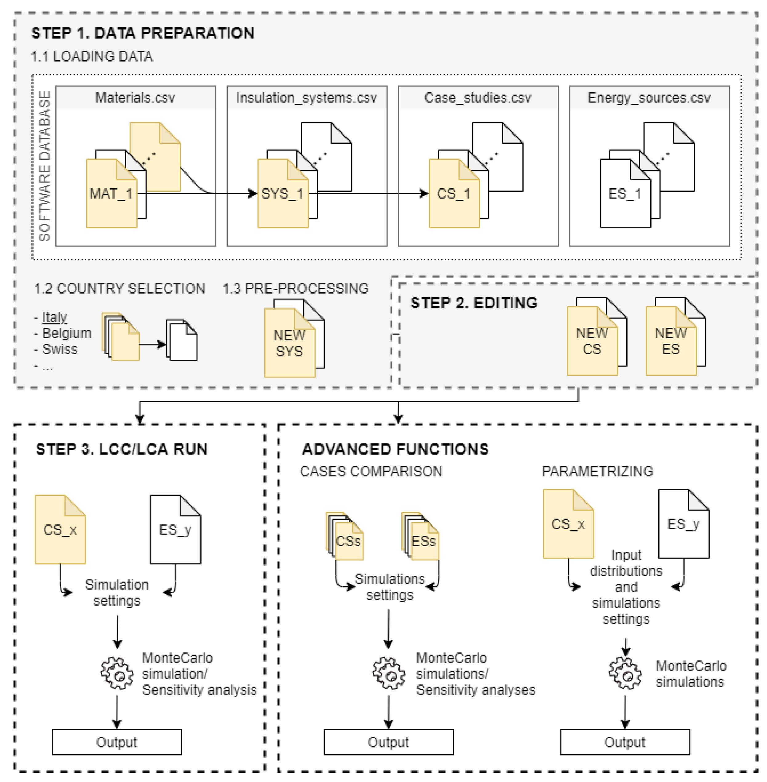
Figure 1 schematically displays the workflow of a generic sustainability assessment within the LCC/LCA software tool. This workflow is based on the reactive programming paradigm of the Shiny package. Within this paradigm, the choice of a specific set of input parameters upstream the workflow influences output choices downstream [18,27] and eases the navigation and setting-up of the case studies. The workflow has been divided into three main steps. At every step, the user can select and tailor specific features of the assessment.

The first step consists of loading the data included in the software database (described later in Section 3.1.2), selecting the reference country, and performing the pre-processing (Section 3.1.3).

The second step consists of visualizing the “case studies” and “energy sources” included in the software database or adding new “case studies” and “energy sources” by inserting the related input data in specific tables (Section 3.1.4).

After the preparation of the case study, the third step consists of the actual LCA/LCC assessment (Section 3.1.5), i.e., in both the stochastic LCC and LCA calculations as well as their sensitivity analyses. The user can select to perform either a LCC, a LCA, or both assessments sequentially. After the calculation of LCA/LCC indicators, SA can be used to inspect the sources of uncertainty of the indicators produced. Once any or both the LCA/LCC assessments are accomplished, results and input data can be downloaded in .csv format. Moreover, results can be directly visualized with the tool.

When many alternative LCA/LCC assessments are needed altogether, the user can exploit the “advanced section” functionalities (Section 3.1.6). These functionalities allow the user to set up in a single step many different case studies and then to launch them sequentially or in parallel. There are two main advanced functionalities: the first one allows the full specification of multiple case studies with their parameter uncertainties and scenario assumptions; the second one, following Lacirignola et al. [28], allows the user to define different comparable probability distributions for each input parameter of a single case study instead. Each step of the workflow is explained in the next subsections, while the complete user-guide of the RIBuild WP5 LCA/LCC Tool (the RIBuild project’s version, available on-line) is provided as Supplementary Materials.

3.1.2. Internal LCC/LCA Database

The software includes a detailed database of input data of Equations (1) to (7) related to the design options (renovation materials and systems) and the energy scenarios. They are organized in four data tables (.csv), named materials, insulation systems, case studies, and energy sources, which can eventually be manually modified and must be included in the software folder. The name of the database insulation system was adopted in the original version of the software within the RIBuild project. However, this database can include data referring to any building “renovation” system. Therefore, from now on we refer to it as systems.

The data frame materials include the LCA data inputs of the materials that can be combined to create a building renovation “system”, as the materials’ mass, their service life, and their unitary environmental impact at the manufacturing and EoL stage. In this regard, the unitary environmental impacts can be provided according to three environmental impact indicators that can be established by the user. The maximum number of impact indicators that can be contained in the materials data frame is three at a time, but the user can “duplicate” the material and includes different indicators for further assessments.

The data frame systems include information on the materials composing a specific renovation system and contain the input data for the LCA/LCC analysis of systems, as the investment cost, the maintenance cost, and the service life. A set of systems can be combined to create one or several building renovation case studies. One or more case studies can be assessed, in terms of LCA/LCC, under one or more possible energy sources scenarios.

The data frame case studies then include information on the energy need and the overall efficiency of HVAC. Finally, the data frame energy sources include data as the energy tariff and the unitary environmental impact of the energy carrier. As for the material data frame, the maximum number of impact indicators that can be contained in the energy source data frame is three.

Each item in the data frames, i.e., each material, system, case study, or energy source, is identified by a name and an ID and is related to a specific Country. Uncertainty characterization of the input parameters included in the four data tables is provided in the form of fully specified background probability distributions (that can be normal, uniform, gamma, Weibull, lognormal, triangular, or single points). At this aim, specific cells of the data frames are filled with information on the distribution shape and parameters.

The following

Table 1. LCA input data included in the 4 data frames of the software database.

LCA Stage (EN 15978 Nomenclature)		LCA Parameter	Data Frames
			Materials	Systems	Case Studies	Energy Sources
Production stage (modules A1–A3)	Material	mk (kg)		x
		UIk (unit of indicator)	x
Use stage (modules B2, B4 and B6)	Maintenance	slk (years)	x
	Replacement	SLj (years)		x
	Energy need	$Q_H^{pre}$, $Q_H^{post}$(kWh/year)			x
	Energy impact	$E{I}_i$(unit of indicator)				x
EoL stage (modules C1-C4)	EoL material impact	EOLk (unit of indicator)	x

and

Table 2. LCC input data included in the 4 data frames of the software database.

LCC Category (EN 15459 Nomenclature)		LCC Parameter	Data Frames
			Materials	Systems	Case Studies	Energy Sources
Investment Cost		CIj (€)		x
Running Cost	Replacement cost	$S{L}_j$(years)		x
		$C{S}_{j, t}$(€)		x
	Maintenance cost	CMj,i (€/year)		x
	Energy cost	$Q_H^{pre}$, $Q_H^{post}$(kWh/year)			x
		${\eta }_{H }$(-)			x
		$EnT$(€/kWh)				x

summarizes the input data of the LCA and LCC assessment, as described in Section 2.1 and Section 2.2, specifying the data frame where the input is included. Instead, further details on the software database organization and the complete four data frames filled with input data related to the case studies analyzed in Section 3.2 are reported as Supplementary Materials.

The macroeconomic variables entering the LCC (Section 2.3) are part of the software database but cannot be manually modified by the user.

Given the original scope of the birth of the tool (the EU project RIBuild), the actual input data, included in the data frames of the software version freely available in the project website, are mainly related to internal insulation solutions and are referred to specific EU Countries where these solutions are implemented. Their background probability distributions have been defined in national contexts using available product-specific data provided by companies producing market-available insulation systems [19,29].

3.1.3. Loading Data, Country Selection, and Pre-Processing

At the start-up, the software tool automatically aggregates the environmental impacts from the material level to the system level for each system, using the information contained in the materials and systems tables. The aggregate impacts are obtained by multiplying the masses of the materials composing each system by their corresponding unitary impacts in the considered LCA stages (Equations (2)–(4)).

The empirical distributions of impacts at the system level will generally have an unknown formula, being the sum of a small number of different probability distributions (limiting theorems, such as the Central Limit Theorem (CLT), do not apply due to the low number of distributions). Therefore, these distributions are obtained numerically by sampling from the distribution of masses and unitary impacts. To simplify calculations down the workflow and to minimize memory usage, these unknown distributions computed numerically are then approximated by distributions with known formulas using maximum likelihood estimation (MLE). Thus, for each environmental indicator, a selection of known distributions is alternatively used to fit these environmental impacts at the system level, and the ones associated with a higher maximized log-likelihood are selected as best approximations to these unknown distributions.

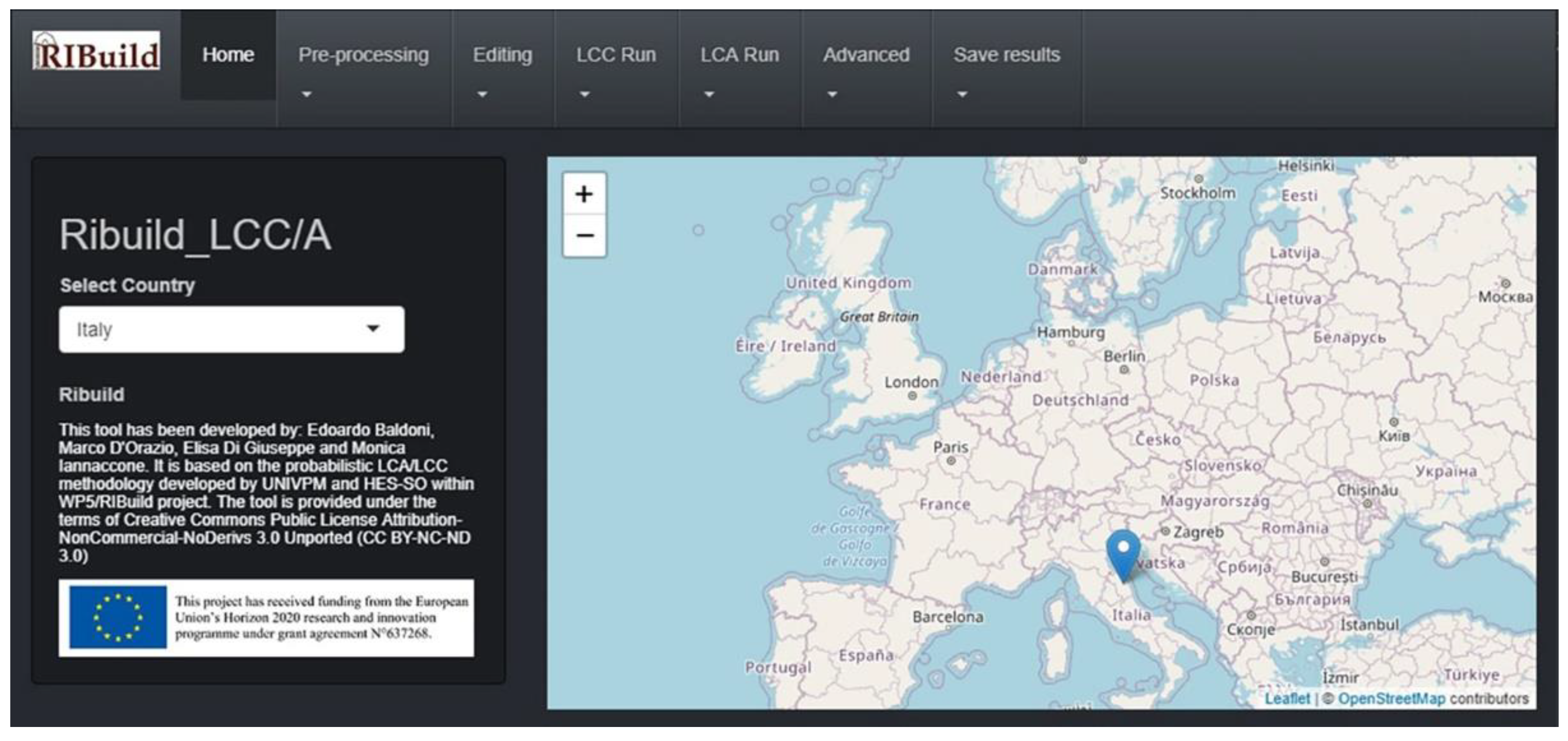
After the data loading step, the GUI is opened (Figure 2). The “Home” page allows the user to select the Country of the case study. With this selection, the user drills down into the subset of the internal database that is relevant to the assessment (i.e., for each data frame, only the items referred to that specific country can be selected). Due to the reactive programming paradigm, the subsequent choices of case studies and energy sources will be influenced by this initial choice of the Country.

The “Pre-processing” tab contains a series of functionalities to visualize the loaded data on systems and the input data of the economic scenarios, and to perform a specific calculation of the heat transmission loss through a wall, based on the annual heating degree-day (HDD) as explained in [15], if needed (for instance, for assessments at the wall level, as in the RIBuild project). An important component of the pre-processing tab is the possibility to browse the available materials and use them to create new systems. Further details on all the functionalities of the “Pre-processing” menu are provided in the software user guide as Supplementary Materials.

3.1.4. Editing of Case Studies and Energy Sources

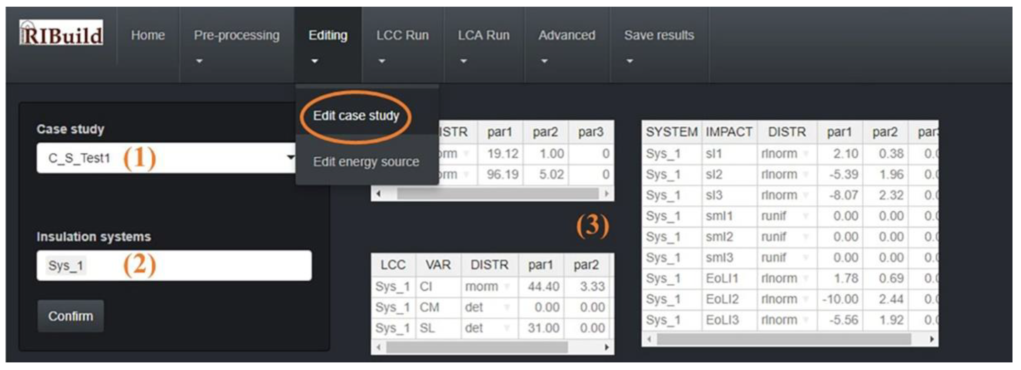
The “Editing” step is the core of the design of the sustainability assessments. This stage allows the selection of the case studies and the energy sources among the available ones, shows the probability distributions of the main inputs related to them, and allows their editing (Figure 3).

Distributions and parameters of each case study are defined at the start-up in the internal database. However, the software allows for the flexible use of this information and the combination of different input parameters, with their distributions, into newly generable case studies and energy sources. Indeed, new case studies and sources can be created within the GUI in the “Editing” tab.

The distributions of the input data of the case study (under the “Edit case study” tab) are divided into three groups: the energy need before and after renovation ($Q_H^{Pre}$ and $Q_H^{Post}$), the cost-related system (CI, CM, SL, the latter used for both LCA and LCC), and impact-related distributions ($s{I}_i$, $sm{I}_i$, $Eo{L}_i$). In the “Edit energy source” tab, it is possible to visualize and modify the inputs related to the energy scenario, i.e., EnT, EnFc, ${\eta }_H$, $E{I}_i$ (EnFc is a multiplying factor that can be used for the energy performance in Equations (1) and (5)). From Figure 3, it can be noticed that any input data of the assessment is associated with a specific distribution (DISTR) that, in turn, is described by up to three specific parameters (par1, par2, par3) representing the shapes and ranges of the distributions. A new case study or energy source can be generated, and the user is allowed to edit manually every single input parameter of the assessment. Both distributions and distributions’ parameters can be adjusted to tailor this new case study or source and to model a wide range of specific interventions.

3.1.5. LCA/LCC Run

The tab “LCC run” allows the user to compute GC and PB, deriving a series of summary statistics and also performing the sensitivity analysis. The LCC indicators are computed using the formulas provided in Section 2.2 with the MC approach described in Section 2.4.

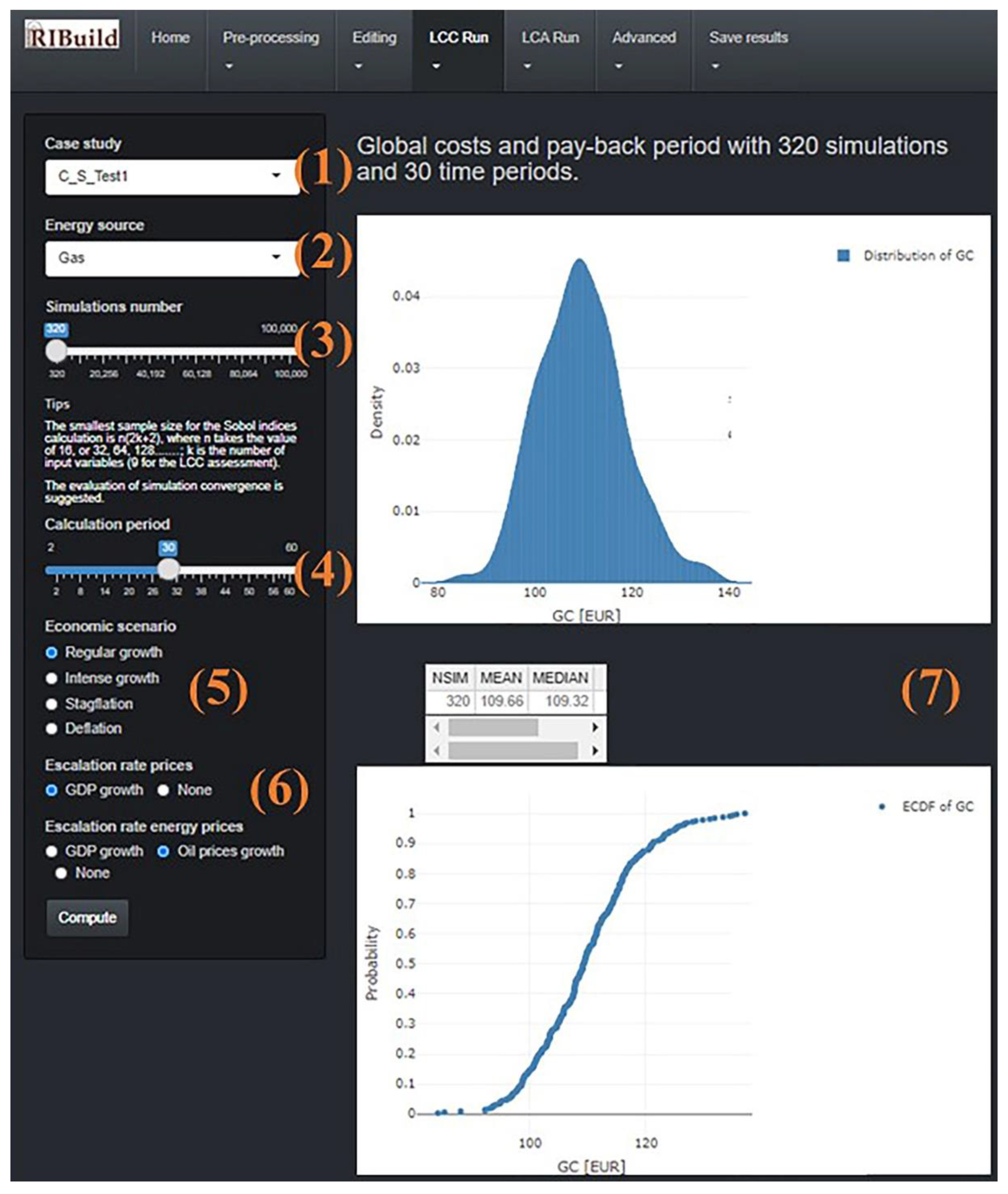
In the “LCC analysis” subtab (Figure 4), the last set of input parameters needed to run the assessment can be chosen. These refer to the specific energy source scenario involving carrying out the LCC, the number of simulations (for convergence purposes), the calculation period, the economic scenario among the available ones (see Section 2.3), and different assumptions on escalation rates of prices of energy and of human operation [16]. After having chosen these final input parameters, the assessment can be run. At accomplishment, outputs and summary statistics are reported (as shown later in Section 4).

To inspect the sources of GC uncertainty, the user can perform the SA using the “LCC—sensitivity analyses” subtab, after having run the LCC calculation. Two versions of the sensitivity analysis are implemented: according to “Method 1”, the SA is carried out for all inputs including macroeconomic variables, to evaluate the influence of their uncertainty on the result. With this method, it is possible to compare the importance of economic inputs across different macroeconomic scenarios.

In “Method 2”, the SA is performed to focus on the influence of the LCC inputs uncertainties, except for macroeconomic variables. This approach is useful if the user is interested in comparing the performance of several design options which are subjected to the same macroeconomic scenario uncertainties, by assessing the influence on the output variance given by other factors as investment costs, service lives, energy tariffs, etc.

In this case, alternative trajectories of the three macroeconomic variables are simulated, and, for each simulation, the Sobol’s sampling is performed only on the other LCC parameters, in order to assess the eventual variation of the sensitivity indices. The graphical output of a sensitivity assessment using the two methods is presented in the following Section 4.

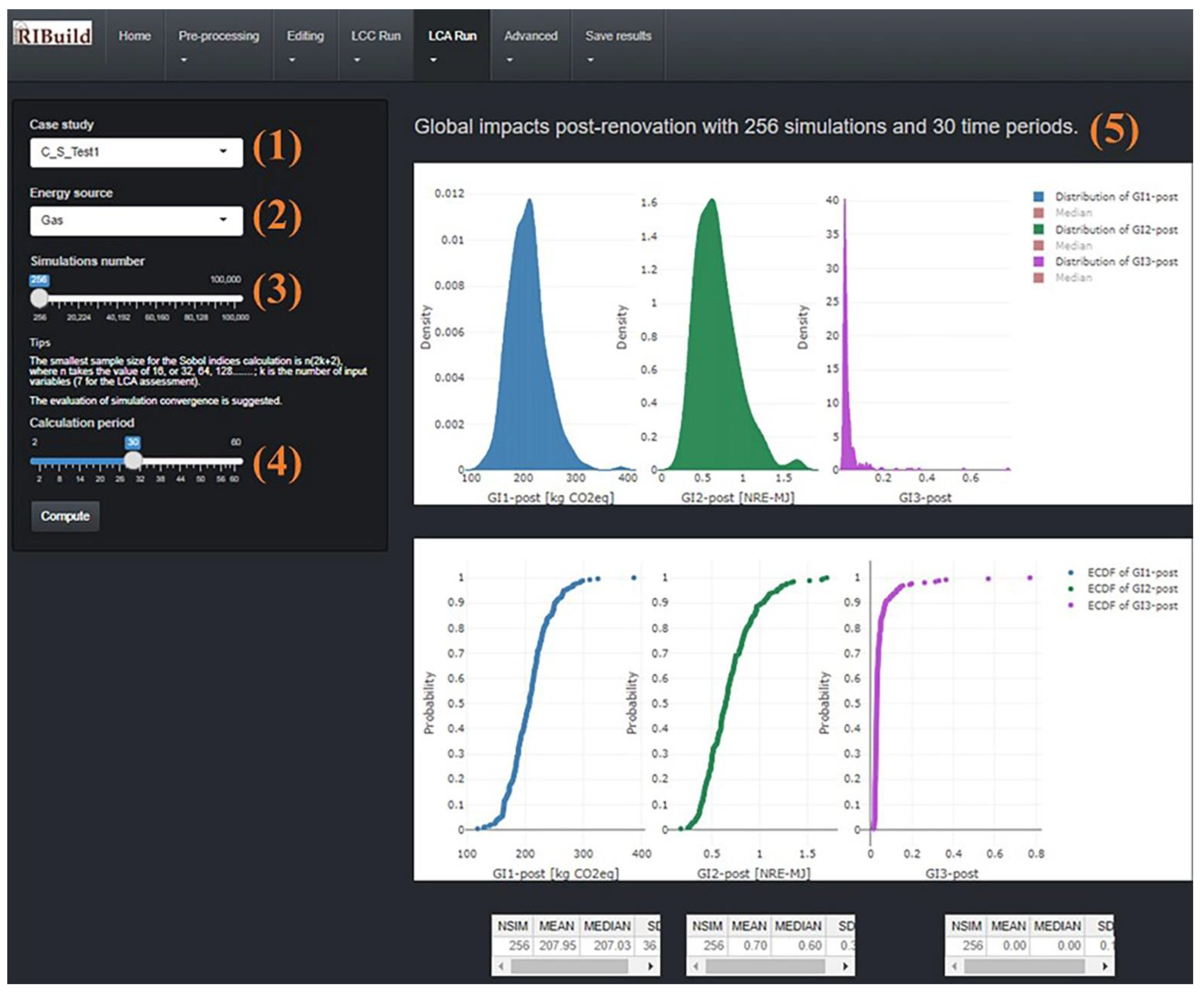
Analogously to the LCC assessment, the “LCA run” tab allows computing LCA indicators and their sensitivity analysis. In the “LCA” subtab (Figure 5), the user specifies the energy source scenario for the assessment, the number of simulations, and the calculation period. Outputs of the calculation procedures are provided on the right-hand side of the panel where distributions and summary statistics of post-renovation, pre-renovation impacts together with the corresponding impacts savings are presented (as shown later in Section 4). As regards the LCA, three environmental impact indicators can be computed, depending on the related input data provided by the user. Sensitivity analysis for LCA assessments is available for all the three environmental indicators using the same “Method 1” available for LCC assessments.

3.1.6. Advanced Functions

When the number of comparisons grows, the steps described above can become onerous. To facilitate the comparison of large numbers of different case studies, some advanced functionalities have been developed and made accessible.

These functions allow the user to set up many different case studies and then to launch them sequentially or in parallel. There are two main advanced functionalities: the first one (“Cases comparison” tab) allows the full specification of multiple case studies with their parameter uncertainties and scenario assumptions; the second one (“Parametrizing” tab) allows the user to define different probability distributions for each input parameter of a single case study, following Lacirignola et al. [28].

In the tab “Cases comparison”, the left-hand panel allows the user to select multiple case studies, multiple energy sources, a range of simulation numbers, a range of calculation periods, multiple economic scenarios, and escalation rates, obtaining a matrix of all the combinations of cases. As the number of case studies generated can become easily large, the user can specify a parallelization method to speed up calculations: the “Simulations” option distributes a number of MC simulations for each case study to the nodes of the calculation cluster, while the “Case Studies” option distributes entire case studies to the nodes. The first parallelization option is recommended when dealing with few case studies characterized by a very large number of MC simulations while the second option is recommended when dealing with a large number of case studies.

The tab “Parametrizing” allows the user to define different probability distribution shapes for each input parameter of a single case study, and it is considered particularly useful when dealing with novel products whose uncertainty characterization might have been based on a small number of data points and assumptions [28]. The normal, the uniform, and the triangle (both left and right) distributions are available choices for the user to characterize input data. The generation of these distributions with comparable support but different assumptions about their associated probability is done following Lacirignola et al. [28].

3.2. Exemplary Applications

In order to demonstrate the software potential, illustrative examples of the application of the stochastic LCC and LCA are provided in the next sub-sections, using the different software functionalities: a single assessment (Section 3.1.5), multiple assessments of several case studies under alternative scenarios (through “cases comparison”), the analysis of the impact of different PDFs shapes (through “parametrizing”). Five internal thermal insulation measures, applied in a historic building in Italy for its energy efficiency improvement, are assessed and compared, also considering alternative energy (for LCA and LCC) and economic (for LCC) scenarios. The simulation input data are included in the database of the software version of the RIBuild website, and the specific data frames are reported as Supplementary Materials.

3.2.1. The Case Studies

The five insulation systems mainly differ for the insulation material adopted, i.e., Expanded Polystyrene (EPS), Calcium Silicate (CaSi), Autoclaved Aerated Concrete (AAC), Cork, and Rockwool (RW). A detailed description of the stratigraphy of each system and the thermophysical properties of each layer can be found in [15].

The systems are applied to a typical Italian historic building placed in the Italian region Lombardy (2200 < HDD < 2900), made of 30 cm thick plastered solid bricks masonry walls characterized by an air-to-air heat transfer coefficient (U-value) of 1.76 W/m²K. The thicknesses of the different internal insulation layers were calculated to achieve a similar U-value for the retrofitted walls, i.e., equal to or slightly lower than 0.36 W/m²K, according to the actual Italian law requirements [30], with slight differences due to the commercial insulation thicknesses available in the market.

Two alternative “building heating systems”, i.e., “energy scenarios”, have been considered, i.e., a gas boiler and an air-to-water heat pump (“natural gas” and “electricity” energy scenarios in the following), which are the most widespread in Italy for existing buildings.

The functional unit for both LCC and LCA is defined as the insulation intervention needed to cover a wall area of 1 m² and to obtain an average U-value ≤ 0.36 W/m²K with the minimum insulation thickness and for a calculation period of 30 years, assumed equal to the service lives of the insulation systems. For sake of simplicity, no maintenance or replacement operations are considered within this time horizon in these exemplary applications.

Moreover, in this simplified application, as the LCA and LCC are performed at the “component level”; the operational energy use is considered the only heat transmission loss through the wall. Assuming the walls’ U-values as deterministic in both pre- and post-renovation scenarios, the pre- and post-renovation heat transmission losses ($Q_H^{pre}$ and $Q_H^{post}$) are computed as normal distributions through the annual HDD method, considering the variability of the HDD data of the Italian Lombardy region from 2000 to 2016 (extracted from the Eurostat database, [31]).

Concerning the LCC data inputs, the statistical distributions of the investment costs (CI) are defined based on producers’ pricing lists (collected in 2019), considering the wall as clean and ready for the internal insulation installation. The energy tariffs refer to the Italian context [32].

Regarding the LCA, the global warming potential (GWP), acidification potential (AP), and eutrophication potential (EP) indicators of the CML-2001 baseline V3.02/EU25 LCIA method are chosen for comparing the insulation systems since representing the most significant indicators according to [33]. Thus, data from the ecoinvent v.3.1 database were retrieved to characterize the unitary environmental impacts of materials used in the five insulation systems during the production and EoL phases, and of the heating equipment. The PDFs of these unitary environmental impacts for LCI background data are obtained based on the pedigree matrix approach [34], using the MC analysis included in SimaPro software v8.1 (10,000 runs) and a data-fitting procedure (see [15] for further details).

Concerning the masses of the materials, the uncertainty due to the possible differences among provisional and real quantities installed during the renovation is considered. At this aim, a triangular distribution is assigned to each material mass, where the mode is the quantity computed in the project, while minimum and maximum values are defined considering a variation from the mode by −5% to +10% according to [35].

3.2.2. A Single Stochastic LCA and LCC Analysis

The results of a stochastic LCA and a stochastic LCC analysis applied to the EPS case study are reported in this section to illustrate the functionalities of the “LCA run” and “LCC run” tabs of the software. The EPS case study is considered for the analyses, which are carried out assuming a natural gas energy source scenario (in both LCA and LCC) and a regular growth macroeconomic scenario (in LCC). Sensitivity analyses are then realized to identify the most important input parameters for each environmental/economic indicator, through the “LCA—Sensitivity analyses” and “LCC—Sensitivity analyses” tabs. A total of 40,000 runs are realized to ensure a sufficient convergence of the result.

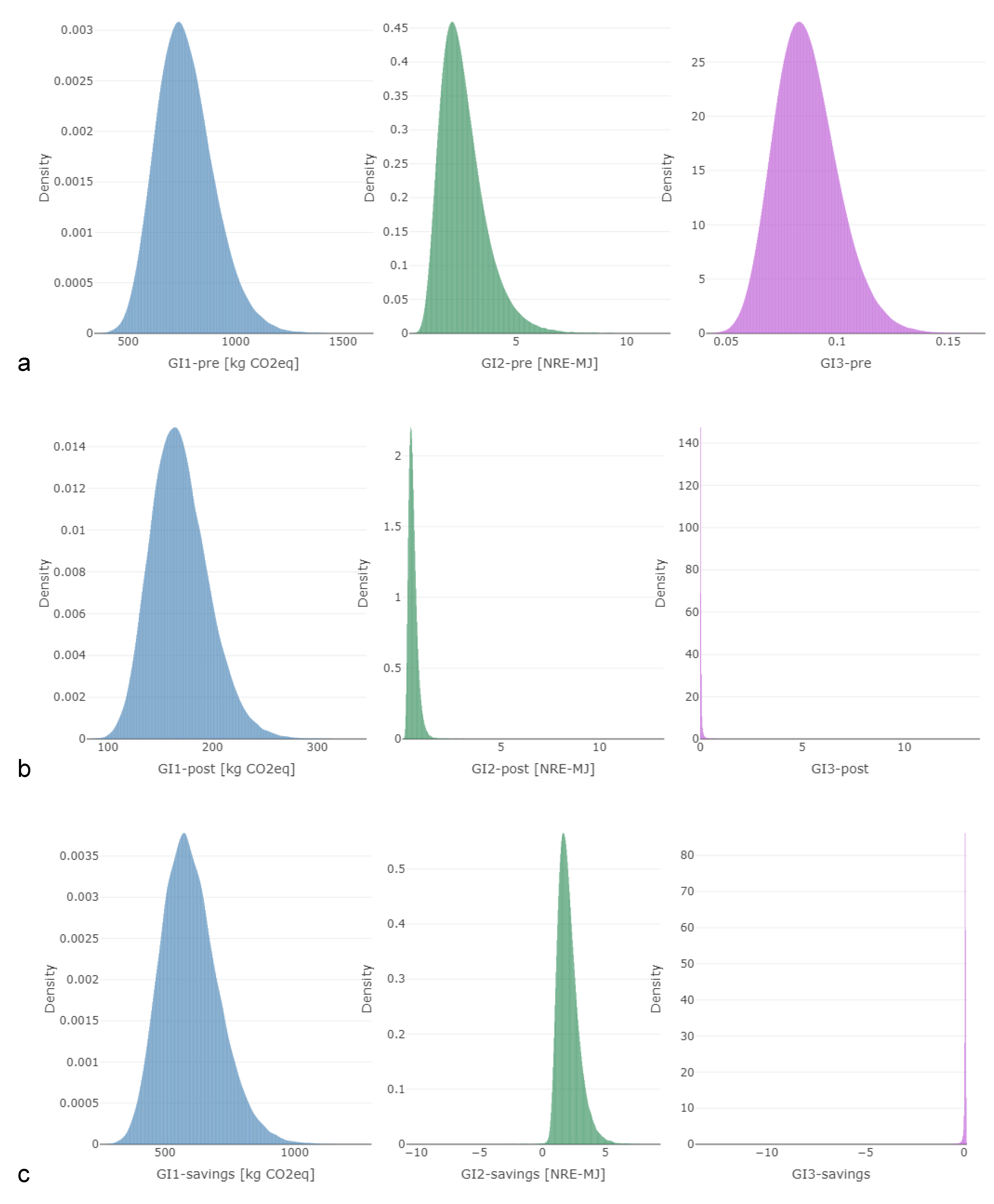
Concerning the LCA, the software calculates, for the selected case study, the distributions of the three environmental impacts in pre- and post-retrofit situations, as well as the related impact savings. Interactive visualization of the results is provided at the end of the analysis in terms of the probability density function (PDF) and cumulative distribution functions (CDF). In Figure 6, the PDFs plotted by the software are reported.

The software also provides synthetic data for describing each stochastic output, such as mean (µ), median (χ), and standard deviation (σ), in addition to the possibility to export the entire dataset as a .xlsx file. In particular, in terms of mean values, the installation of the EPS insulation system in the building case study allows for reducing the GWP from about 767 to 169 kg for the CO₂-Eq., the AP from about 2.63 to 0.55 kg for the SO₂-Eq., and the EP from 0.09 to 0.05 kg for the (PO₄)³-Eq. It should be noted that mean values are not always significant, especially in the case of the distribution that substantially differs from the normal one, as in the case of the EP indicator (see Figure 6).

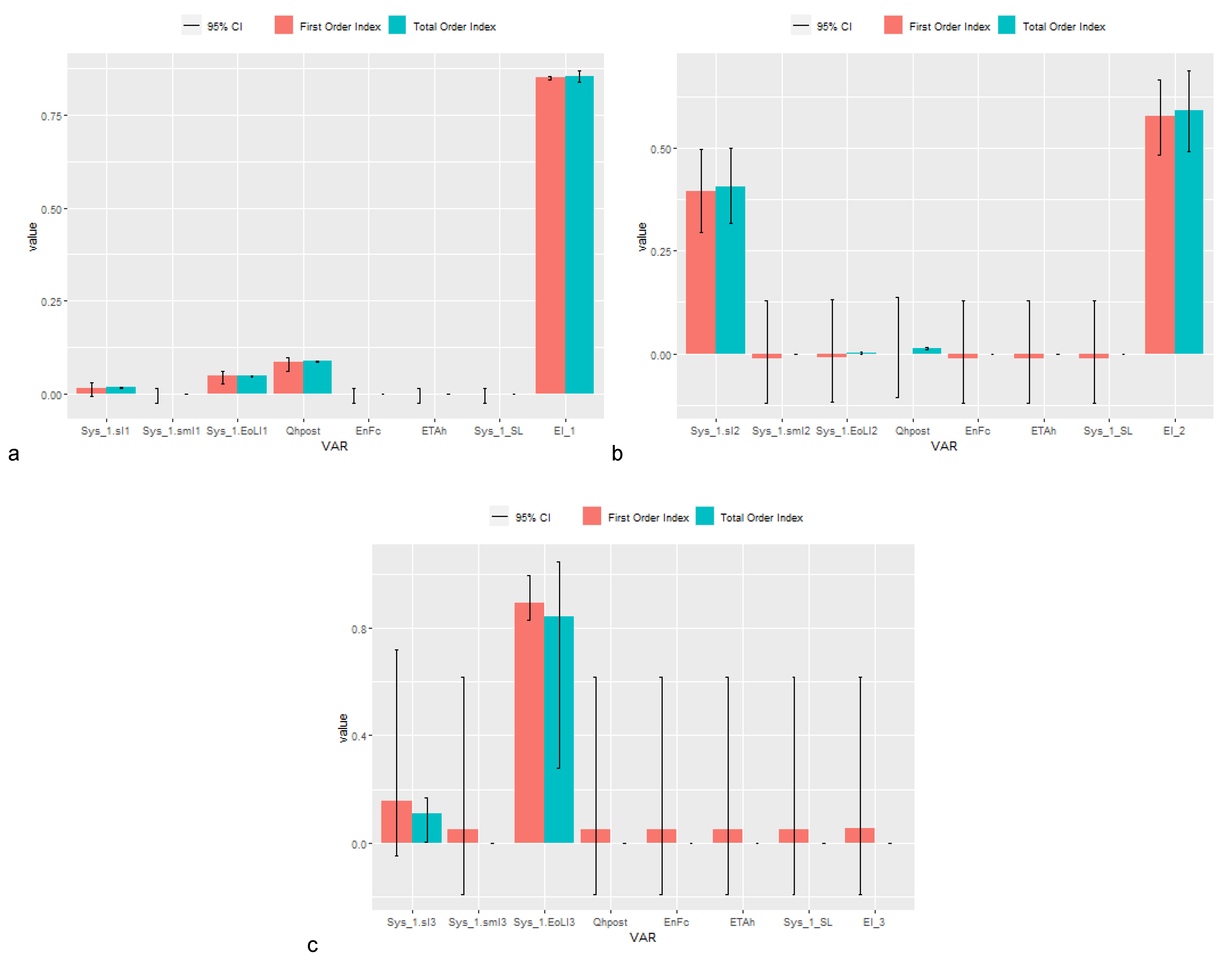
A sensitivity analysis has been carried out to investigate how the uncertainty on input values affects the uncertainty on output values. In Figure 7, the first order and total order sensitivity indices obtained for the EPS case are reported as plotted by the software, where it can be noted that no differences are present between the two index types, denoting a low or null interaction between inputs. For the GWP, the highest total order index is obtained for the EI (energy-related impact), showing that uncertainty on EI has the highest impact on GWP uncertainty. EI has also the greatest impact on AP uncertainty, followed by sI (insulation system impact). Finally, concerning the EP, the highest indices are obtained in this case for the EoL (End of Life impact of the system), followed by sI.

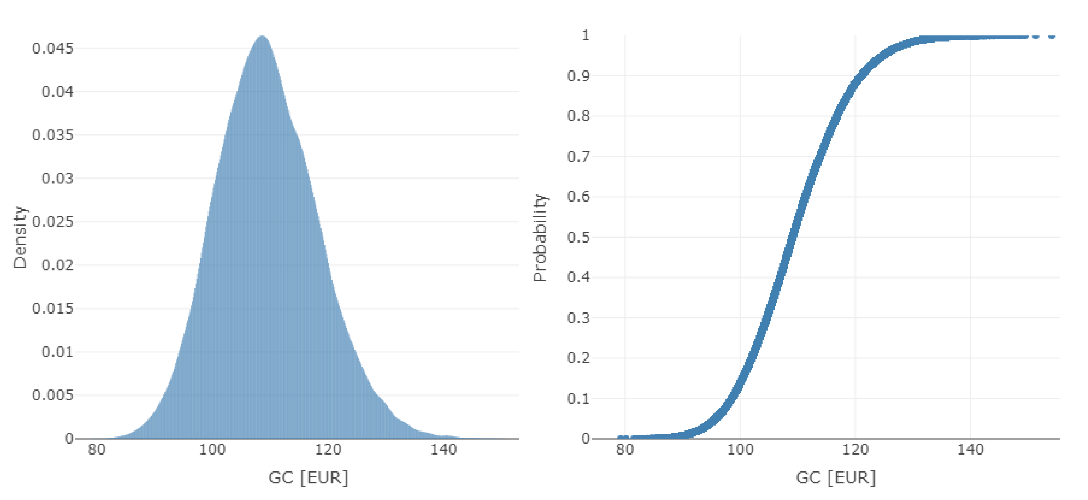
For the LCC analysis (through the “LCC run” tab), the software calculates the stochastic global cost (GC) and payback period (PB) for the selected insulation measure over the defined calculation period. Even in this case, interactive visualization of the stochastic output is provided by the software in terms of the probability density function (PDF) and cumulative distribution functions (CDF). In Figure 8, the PDF and the CDF plotted by the software for the GC and PB are reported. As already seen for the LCA, also in this case, the software provides synthetic data for describing the obtained stochastic output, such as mean (µ), median (χ), and standard deviation (σ), in addition to the possibility to export the entire dataset as a .xlsx report file for further analysis. In this case, the global cost is characterized by a µ of about 110€ (σ = 8.85€), resulting in a mean payback period of 5.30 years (σ = 0.60 years).

Finally, also, the share of investment, maintenance, and energy cost are computed by the software. In terms of mean values, the investment cost is about 40% of the global cost, with a standard deviation of 3.4%.

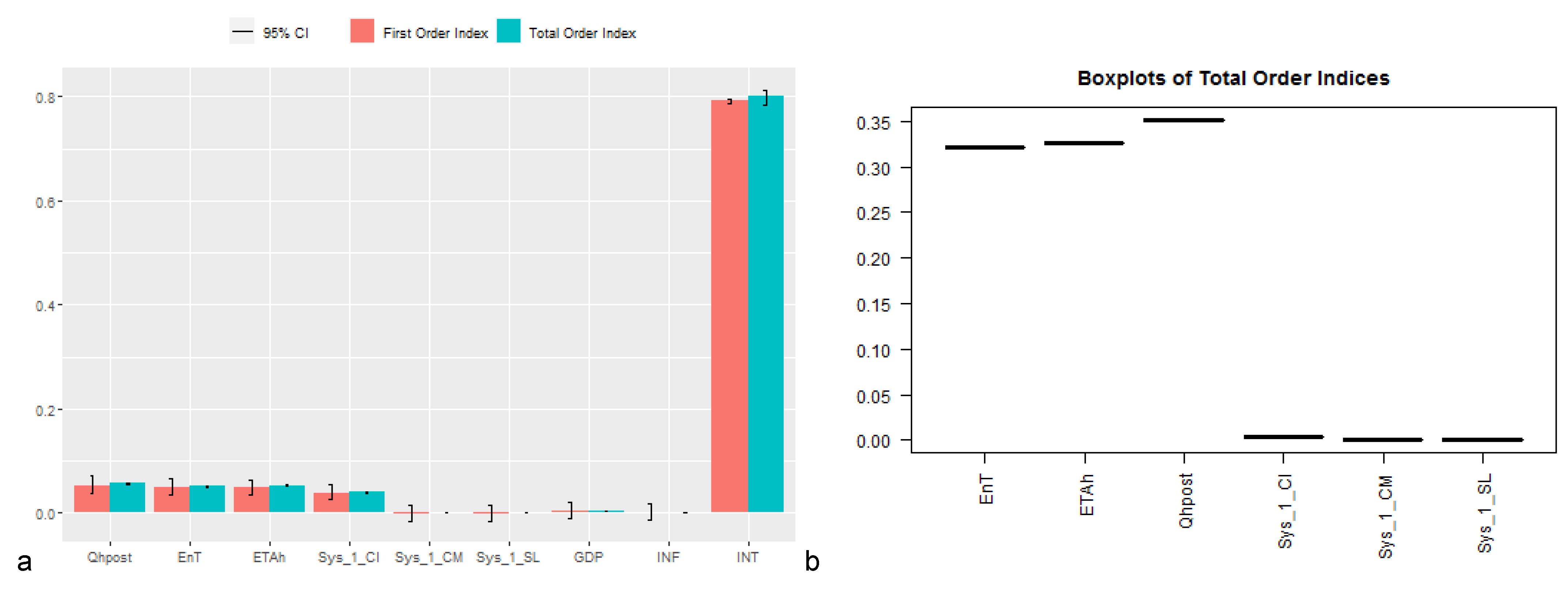
For the LCC analysis, the software provides the sensitivity analysis by following the two different approaches, as seen in Section 3.1.5. In the first approach (“Method 1”), the software computes the sensitivity indices of all the LCC variables, including the macroeconomic ones (inflation rate, interest rate, and growth in GDP). In the second approach (“Method 2”), the software generates alternative trajectories of the three macroeconomic variables (trials) and computes the sensitivity indices of all the remaining variables for each trajectory. In this exemplary application of the software, the result of both approaches is shown, considering 50 trials for method 2.

In Figure 9, the sensitivity indices obtained through the two different approaches are reported as plotted by the software. The highest index for “Method 1” is obtained for the INT parameter, followed by Qhpost, EnT, and ETAh. In “Method 2”, since the sensitivity on the INT parameter is not included in the assessment, the highest indices are obtained for Qhpost, EnT, and ETAh.

3.2.3. LCA and LCC Analysis under Alternative Scenarios

In this section, an exemplary application of the “Cases comparison” tab of the software is shown to demonstrate the ability of the software to support the designers in the selection of the best performing solution under several conditions and eventually evaluate the robustness of the results. At this aim, the environmental and economic indicators obtained for the five insulation systems under different assessment scenarios (different energy sources and macroeconomic scenarios) are compared in the following.

Concerning the LCA, in

Table 3. Mean (µ), median (χ), and standard deviation (σ) of GWP, AP, and EP indicators obtained from the LCA analysis for the natural gas energy source scenario.

Case Study	GWP (kgCO2-Equation)			AP (kgSO2-Equation)			EP (kg(PO4)3-Equation)
	µ	χ	σ	µ	χ	σ	µ	χ	σ
Pre	7.68 × 102	7.56 × 102	1.34 × 102	2.63 × 100	2.44 × 100	1.03 × 100	8.63 × 10−2	8.52 × 10−2	1.43 × 10−2
EPS	1.69 × 102	1.67 × 102	2.75 × 101	5.53 × 10−1	5.09 × 10−1	2.64 × 10−1	4.60 × 10−2	2.39 × 10−2	1.39 × 10−1
CaSi	2.46 × 102	2.43 × 102	3.81 × 101	7.75 × 10−1	6.00 × 10−1	1.23 × 100	1.24 × 10−1	3.30 × 10−2	7.84 × 10−1
AAC	1.82 × 102	1.80 × 102	3.04 × 101	5.95 × 10−1	5.05 × 10−1	8.09 × 10−1	7.66 × 10−2	2.37 × 10−2	5.19 × 10−1
Cork	1.83 × 102	1.80 × 102	2.86 × 101	6.04 × 10−1	5.20 × 10−1	6.26 × 10−1	6.85 × 10−2	2.77 × 10−2	2.73 × 10−1
RW	1.67 × 102	1.65 × 102	2.75 × 101	5.44 × 10−1	4.95 × 10−1	2.79 × 10−1	5.74 × 10−2	2.65 × 10−2	1.92 × 10−1

, the results obtained according to the three selected indicators under the natural gas energy scenario are synthetically reported. Almost all the insulation systems allow a reduction in terms of GWP, AP, and EP during the calculation period, compared to the pre-renovation situation. In terms of both GWP and AP impact indicators, the higher reduction is obtained through the RW insulation system, followed by EPS, AAC, Cork, and CaSi. Regarding the EP impact indicator, instead, the best option is represented by the EPS insulation system, followed by RW, Cork, AAC, and CaSi. In this latter case (CaSi), the overall mean value for EP is even higher than the mean value obtained in the pre-renovation scenario, denoting the possibility to increase the EP if this type of internal insulation solution is adopted.

Table 4. Mean (µ), median (χ), and standard deviation (σ) of GC, PB, CI share, and energy costs’ share obtained from the LCC analysis for the natural gas energy source scenario and regular growth macroeconomic scenario.

Case Study	GC (€)			PB (Years)			CI (%)			Energy (%)
	µ	χ	σ	µ	χ	σ	µ	χ	σ	µ	χ	σ
EPS	109.55	109.14	8.79	5.33	5.00	0.63	39.47	39.44	3.46	60.53	60.56	3.46
CaSi	282.33	282.13	18.10	25.89	24.00	14.49	75.77	75.88	2.66	24.23	24.12	2.66
AAC	151.25	151.03	10.24	9.97	10.00	1.26	58.17	58.21	3.57	41.83	41.79	3.57
Cork	165.15	164.82	10.90	11.40	11.00	1.46	61.00	61.15	3.42	39.00	38.85	3.42
RW	122.05	121.68	8.85	7.05	7.00	0.85	49.84	49.92	3.64	50.16	50.08	3.64

reports the synthetic LCC results obtained for each case study. A similar ranking to that obtained in the LCA analysis is obtained in this study. In terms of mean values, the EPS provides the lowest global cost, followed by RW, AAC, Cork, and CaSi. Since running costs, such as maintenance and energy costs, are almost the same for all the insulation solutions (the first equal to 0 for all the cases, and the second almost the same due to the similar U-values), the differences between the insulation systems obtained in this study can be attributed to the different initial investment costs (CIs).

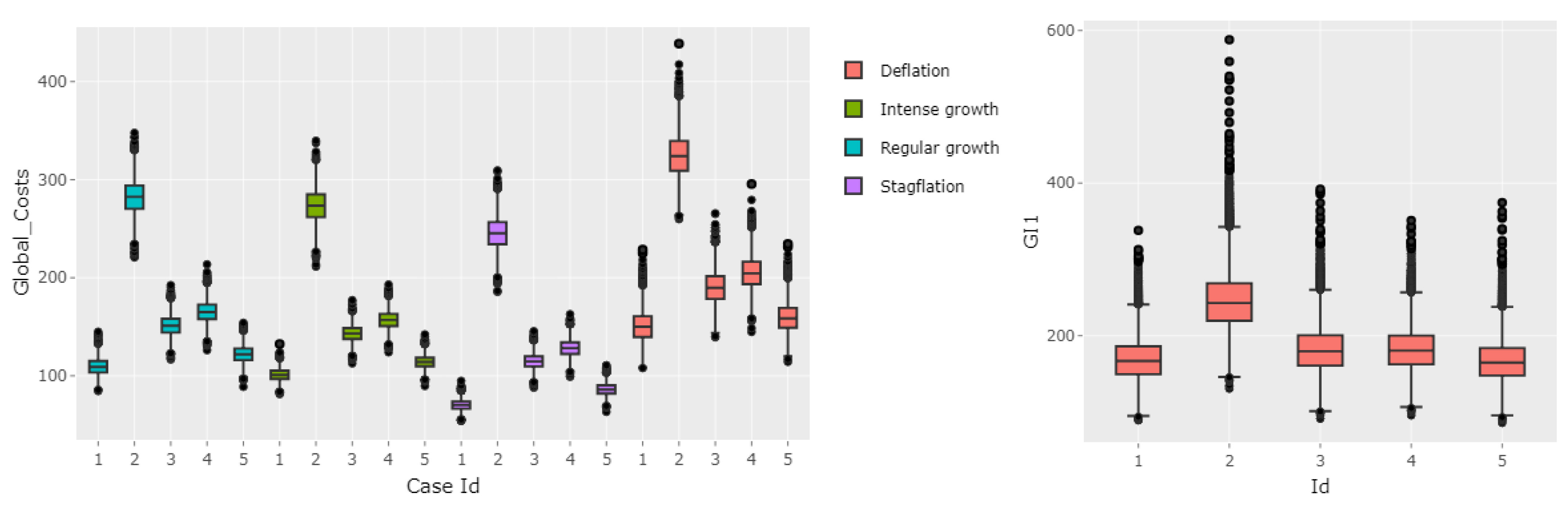
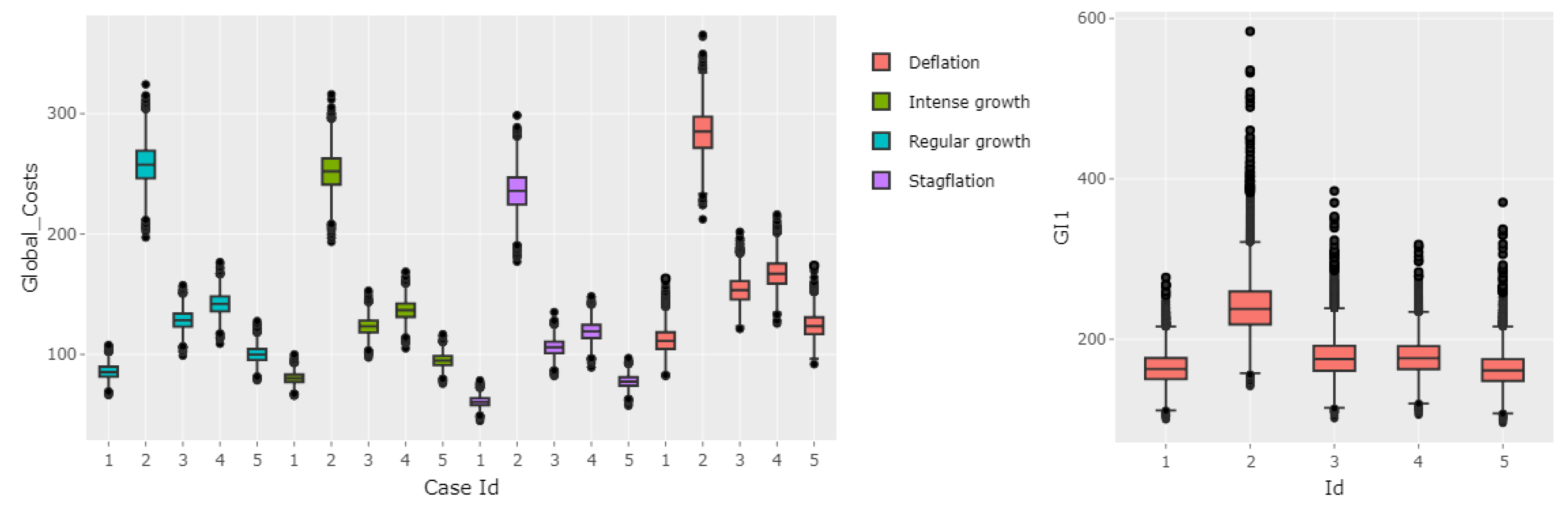
In Figure 10 and Figure 11, the global costs obtained in the different economic scenarios and the GWP are shown for the natural gas and electricity energy source scenarios, respectively. For both the LCC and LCA, the ranking of the solutions obtained for the “natural gas” scenario is confirmed also for the “electricity” energy source scenario: EPS and RW solutions are the best performing solutions from both the economic and the environmental point of view. In the “electricity scenario”, however, lower GC values are generally obtained, mainly due to the higher efficiency of the heat pump (LCC and LCA) together with the lower energy tariff (LCC).

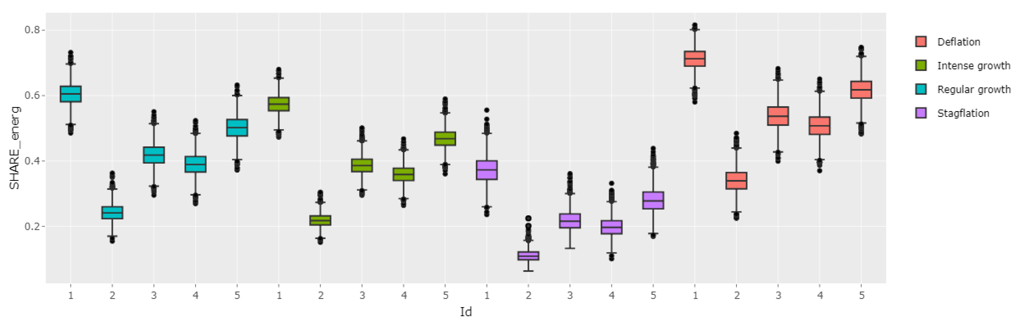
In the LCC calculations, similar results are obtained for the regular and intense growth scenarios. The highest and lowest GCs are instead obtained in the stagflation and deflation scenarios, respectively. This is an expected result. In fact, in the stagflation scenario running costs are generally lower due to the low price development rates, lower than 1, and a discount factor higher than those of all other macroeconomic scenarios (due to the high inflation rate). Conversely, the deflation scenario is characterized by higher running costs, due to an inflation rate lower than those of all the other scenarios and discount rates and escalation factors higher than in other scenarios. This can be also observed in Figure 12, where the energy costs’ share on the GCs are also reported as plotted by the software.

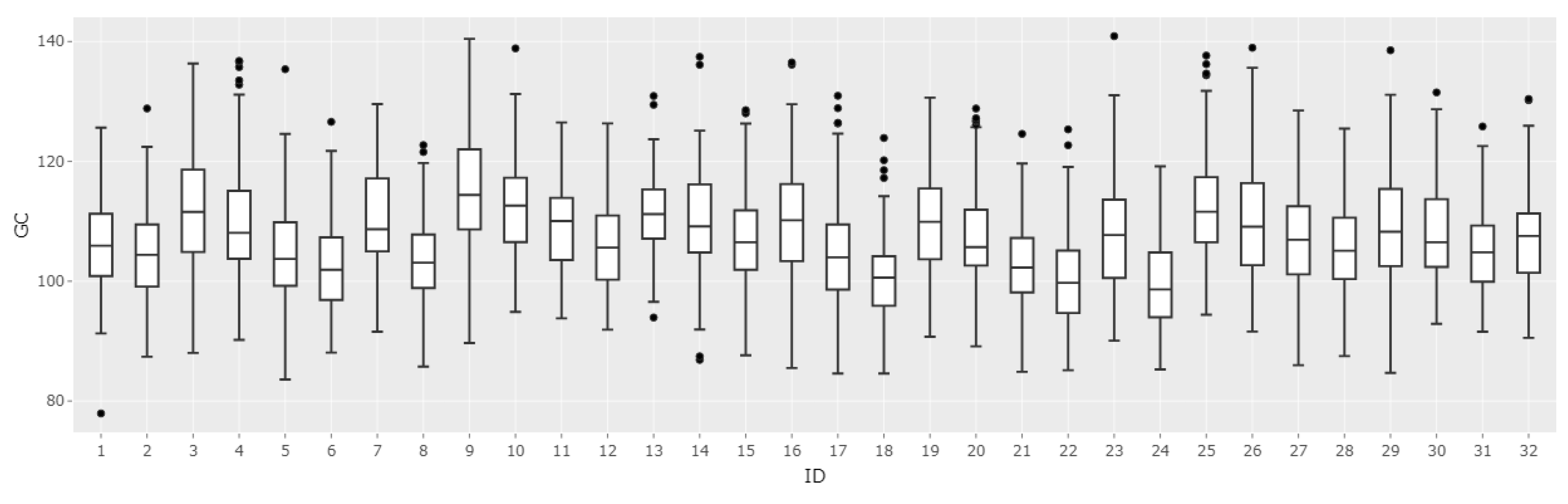
3.2.4. Parametrizing Function

An exemplary application of the “Parametrizing” tab of the software is shown in this section, aimed at evaluating how different assumptions on the probability distribution shape of input parameters may affect the result. At this aim, the LCC analysis of the EPS-based internal insulation system under the regular growth macroeconomic scenario is carried out again, considering, for each input parameter, two different distribution typologies, i.e., a normal and a left-triangular distribution. As a result, a total of 32 stochastic LCC analyses have been obtained from the combination of the different distributions. The results are summarized in Figure 13. As shown, in this case, a maximum deviation of the median value of about 5% is obtained, demonstrating the robustness of the results under the alternative input distribution assumptions.

4. Discussion and Conclusions

Decision support systems are becoming essential tools to achieve the ambitious environmental and climate policy goals of the EU, especially for energy saving investments in the building sector. In fact, decision making on this type of investments requires complex calculation and involves a wide set of data and parameters on both economic and environmental aspects. Therefore, properly designed, accessible, and easy-to-use software tools, supporting investors in assessing the interventions’ ultimate convenience and the eventual trade-offs between economic and environmental performance, seem particularly attractive.

The present paper presents a novel software tool for the assessments of life-cycle costs and environmental impacts of energy efficiency interventions for buildings. The software combines several advanced functionalities for the calculations of the LCA of the environmental performance and the LCC of a specific retrofit intervention. Although LCC and LCA calculations are implemented according to the internationally agreed standards and the recent literature in the field, the software tool presents some major novelties. Not only does it integrate the implementation of both LCC and LCA calculations, but, more importantly, it takes the stochastic nature of input data fully into account. By analyzing uncertainty propagation via Monte-Carlo methods, the tool is able to capture the intrinsic uncertainties associated to investments under uncertainty and, therefore, to support decision making on long-term planning horizons. The software also includes sensitivity analysis functionalities to assess the contribution of input and scenario assumptions on output indicators.

The software design and functionalities are illustrated through a set of case studies concerning alternative building insulation systems. These examples are presented to highlight the wide range of results and parametrization functions the software can generate and implement. This also corroborates the software flexibility with respect to the range of its possible real-world applications.

These functionalities make it suited for use to a large number of users ranging from academic researchers to private investors and policymakers. The detailed database and the flexibility of modeling complex case studies, while accounting for input parameter and scenarios uncertainties, make it appealing to experienced scientists and researchers with a good knowledge and understanding of LCC and LCA. For those users who may be more interested in the easiness to use, transparency, and the graphical functionalities, the tool is characterized by a simple workflow with pre-set parameters and interactive functionalities to adapt each case study to the users’ level of knowledge, and graphical functionalities for the creation of interactive plots for the simple comparisons of large numbers of alternative investment options.

The aim of this software is to provide the user with the information necessary to take investments decisions under uncertainty in the building sector. For this purpose, LCC and LCA results provided are only meant to guide the user to the optimal choice and not to provide one among many alternative options. In fact, the optimal trade-off between economic and environmental performance will have to be resolved by the user that will need to assign his own specific weighting scheme to each set of indicators provided and make decisions accordingly. This assignment is non-trivial and may depend, among others, on the decision-maker risk aversion, the potential environmental risks linked to local conditions, the absolute and relative values (also in economic terms) of the specific environmental pressure under consideration, and the possible different weights to assign to the economic and environmental assessment and to each environmental pressure. All these factors can be hardly embedded flexibly in a software tool.

Still, a potential extension and research line that could be pursued to facilitate the choice could be represented by an automated search algorithm that would explore all feasible technical solutions starting from the available data and draw a continuous Pareto frontier in the 2D space of environmental and economic performance. Such a Pareto frontier would highlight dominant and dominated solutions and provide the user with a restricted set of potentially original optimal investment options.

References

1. European Commission. A Clear Planet for All–A European Strategic Long-Term Vision for a Prosperous, Modern, Competitive and Climate Neutral Economy; COM(2018) 773 Final; European Commission: Brussels, Belgium, 2018. [Google Scholar]
2. European Commission. The European Green Deal; COM (2019) 640 Final; European Commission: Brussels, Belgium, 2019. [Google Scholar]
3. Von der Leyen, U. A Union That Strives for More. My Agenda for Europe. Political Guidelines for the next European Commission; European Commission: Brussels, Belgium, 2019. [Google Scholar]
4. European Commission Energy Performance of Buildings. Available online: https://ec.europa.eu/energy/en/topics/energy-efficiency/energy-performance-of-buildings (accessed on 3 March 2020).
5. Hamdy, M.; Sirén, K.; Attia, S. Impact of financial assumptions on the cost optimality towards nearly zero energy buildings—A case study. Energy Build. 2017, 153, 421–438. [Google Scholar] [CrossRef] [Green Version]
6. OECD. OECD Guidance on Sustainability Impact Assessment; OECD: Paris, France, 2010. [Google Scholar]
7. Amini Toosi, H.; Lavagna, M.; Leonforte, F.; Del Pero, C.; Aste, N. Life Cycle Sustainability Assessment in Building Energy Retrofitting; A Review. Sustain. Cities Soc. 2020, 60, 102248. [Google Scholar] [CrossRef]
8. Almeida, M.; Ferreira, M. Cost effective energy and carbon emissions optimization in building renovation (Annex 56). Energy Build. 2017, 152, 718–738. [Google Scholar] [CrossRef]
9. Dalla Mora, T.; Peron, F.; Romagnoni, P.; Almeida, M.; Ferreira, M. Tools and procedures to support decision making for cost-effective energy and carbon emissions optimization in building renovation. Energy Build. 2018, 167, 200–215. [Google Scholar] [CrossRef]
10. CEN EN 15459-1:2017 Energy Performance of Buildings–Economic Evaluation Procedure for Energy Systems in Buildings—Part 1: Calculation Procedures, Module M1-14; CEN: Brussels, Belgium, 2017.
11. ISO 14040:2006 Environmental Management—Life Cycle Assessment—Principles and Framework; ISO: Geneva, Switzerland, 2006.
12. ISO 14044:2006 Environmental Management—Life Cycle Assessment—Requirements and Guidelines; ISO: Geneva, Switzerland, 2006.
13. CEN EN 15804: 2011 Sustainability of Construction Works–Environmental Product Declarations–Core Rules for the Product Category of Construction Products; CEN: Brussels, Belgium, 2011.
14. CEN EN 15978: 2010. Sustainability of Construction Works–Sustainability Assessment of Buildings–Calculation Method; CEN: Brussels, Belgium, 2010.
15. Di Giuseppe, E.; D’Orazio, M.; Du, G.; Favi, C.; Lasvaux, S.; Maracchini, G.; Padey, P. A Stochastic Approach to LCA of Internal Insulation Solutions for Historic Buildings. Sustainability 2020, 12, 1535. [Google Scholar] [CrossRef] [Green Version]
16. Baldoni, E.; Coderoni, S.; D’Orazio, M.; Di Giuseppe, E.; Esposti, R. The role of economic and policy variables in energy-efficient retrofitting assessment. A stochastic Life Cycle Costing methodology. Energy Policy 2019, 129, 1207–1219. [Google Scholar] [CrossRef]
17. Baldoni, E.; Coderoni, S.; D’Orazio, M.; Di Giuseppe, E.; Esposti, R. From cost-optimal to nearly Zero Energy Buildings’ renovation: Life Cycle Cost comparisons under alternative macroeconomic scenarios. J. Clean. Prod. 2021, 288, 125606. [Google Scholar] [CrossRef]
18. Di Giuseppe, E.; D’Orazio, M.; Favi, C.; Rossi, M.; Lasvaux, S.; Padey, P.; Favre, D.; Wittchen, K.; Du, G.; Nielsen, A.; et al. RIBuild, D5.1 Report and Tool: Probability Based Life Cycle Impact Assessment; Project No. 637268 European Union’s Horizon 2020; European Commission: Brussels, Belgium, 2017. [Google Scholar]
19. Di Giuseppe, E.; Iannaccone, M.; D’Orazio, M.; Coderoni, S.; Baldoni, E.; Esposti, R.; Favre, D.; Padey, P.; Toczé, M.; Lasvaux, S.; et al. RIBuild, D5.2 Report and Tool: Probability Based Life Cycle Cost; Project No. 637268 European Union’s Horizon 2020; European Commission: Brussels, Belgium, 2018. [Google Scholar]
20. Burhenne, S.; Tsvetkova, O.; Jacob, D.; Henze, G.P.; Wagner, A. Uncertainty quantification for combined building performance and cost-benefit analyses. Build. Environ. 2013, 62, 143–154. [Google Scholar] [CrossRef]
21. Copiello, S. Economic parameters in the evaluation studies focusing on building energy efficiency: A review of the underlying rationale, data sources, and assumptions. Energy Procedia 2019, 157, 180–192. [Google Scholar] [CrossRef]
22. Lütkepohl, H. New Introduction to Multiple Time Series Analysis, 1st ed.; Springer: Berlin/Heidelberg, Germany, 2006. [Google Scholar]
23. Sobol, I.M. Global sensitivity indices for nonlinear mathematical models and their Monte Carlo estimates. Math. Comput. Simul. 2001, 55, 271–280. [Google Scholar] [CrossRef]
24. Sobol’, I.M. On the distribution of points in a cube and the approximate evaluation of integrals. USSR Comput. Math. Math. Phys. 1967, 7, 86–112. [Google Scholar] [CrossRef]
25. Saltelli, A.; Ratto, M.; Andres, T.; Campolongo, F.; Cariboni, J.; Gatelli, D.; Saisana, M.; Tarantola, S. Global Sensitivity Analysis. The Primer; Wiley: Chichester, UK, 2008; ISBN 9780470059975. [Google Scholar]
26. R Development Core Team. R: A Language and Environment for Statistical Computing; R Foundation for Statistical Computing: Vienna, Austria, 2008; ISBN 3-900051-07-0. Available online: http://www.R-project.org (accessed on 5 July 2021).
27. Chang, W.; Cheng, J.; Allaire, J.; Xie, Y.; McPherson, J. shiny: Web Application Framework for R. R Package Version 1.0.3. Available online: https://cran.r-project.org/ (accessed on 5 July 2021).
28. Wan, Z.; Hudak, P. Functional Reactive Programming from First Principles. Sigplan Not. 2000, 35, 242–252. [Google Scholar] [CrossRef]
29. Lacirignola, M.; Blanc, P.; Girard, R.; Pérez-López, P.; Blanc, I. LCA of emerging technologies: Addressing high uncertainty on inputs’ variability when performing global sensitivity analysis. Sci. Total Environ. 2017, 578, 268–280. [Google Scholar] [CrossRef] [PubMed]
30. Ministero dello Sviluppo Economico Decreto Interministeriale 26.06.2015–Applicazione Delle Metodologie di Calcolo Delle Prestazioni Energetiche e Definizione Delle Prescrizioni e dei Requisiti Minimi Degli Edifici; Ministero dello Sviluppo Economico: Roma, Italy, 2015.
31. Eurostat Cooling and Heating Degree Days by NUTS 2 Regions–Annual Data. Available online: https://ec.europa.eu/eurostat/statistics-explained/index.php?title=Heating_and_cooling_degree_days_-_statistics (accessed on 5 July 2021).
32. Di Giuseppe, E.; Maracchini, G.; Gianangeli, A.; Bernardini, G.; D’Orazio, M. Internal Insulation of Historic Buildings: A Stochastic Approach to Life Cycle Costing Within RIBuild EU Project. In Sustainability in Energy and Buildings; Springer: Singapore, 2020; pp. 349–359. ISBN 978-981-32-9868-2. [Google Scholar] [CrossRef]
33. Bueno, C.; Hauschild, M.Z.; Rossignolo, J.A.; Ometto, A.R.; Mendes, N.C. Sensitivity analysis of the use of Life Cycle Impact Assessment methods: A case study on building materials. J. Clean. Prod. 2016, 112, 2208–2220. [Google Scholar] [CrossRef] [Green Version]
34. Mutel, C. Why Does the Ecoinvent Database Love the Lognormal Distribution? 2013. Available online: https://chris.mutel.org/ecoinvent-lognormal.html (accessed on 5 July 2021).
35. Igos, E.; Benetto, E.; Meyer, R.; Baustert, P.; Othoniel, B. How to treat uncertainties in life cycle assessment studies? Int. J. Life Cycle Assess. 2019, 24, 794–807. [Google Scholar] [CrossRef]
Figure 1. LCA/LCC Software workflow.
Sustainability 13 07975 g001
Figure 2. Software Home Page.
Sustainability 13 07975 g002
Figure 3. “Editing” menu. Visualization of the summary data of a case study under the “Edit case study” Table (1) Identification of the case study; (2) Identification of the renovation systems applied to a case study; (3) Visualization/text editing of the input data included in the database.
Sustainability 13 07975 g003
Figure 4. “LCC Run” menu. Visualization of the input parameters needed to run a case study under the “LCC analysis”; Table (1) Identification of the case study; (2) Identification of the energy source; (3) Number of simulations to be run; (4) Calculation Period; (5) Economic scenarios where to perform the LCC assessment; (6) Specific setting for the escalation rates; (7) Graphical outputs and summary statistics at the end of the calculation.
Sustainability 13 07975 g004
Figure 5. “LCA Run” menu. Visualization of the input parameters needed to run a case study under the “LCA”; Table (1) Identification of the case study; (2) Identification of the energy source; (3) Number of simulations to be run; (4) Calculation Period; (5) Graphical outputs and summary statistics at the end of the calculation.
Sustainability 13 07975 g005
Figure 6. PDFs of the GWP (GI1), AP (GI2), and EP (GI3) indicators in pre- (a) and post- (b) renovation scenarios, and impact savings (c) for the EPS internal insulation system.
Sustainability 13 07975 g006
Figure 7. LCA first order and total order sensitivity indices for the EPS case and each impact indicator: (a) GWP; (b) AP; (c) EP. The error bars indicate the confidence level intervals at 95%.
Sustainability 13 07975 g007
Figure 8. PDF and CDF of the global cost obtained for the EPS case considering the natural gas energy source scenario and the regular growth macroeconomic scenario.
Sustainability 13 07975 g008
Figure 9. (a) First order and total order sensitivity indices for global costs computed with “Method 1” for the EPS case; (b) Total order sensitivity indices for global costs computed with “Method 2” for the EPS case. The error bars indicate the confidence level intervals at 95%.
Sustainability 13 07975 g009
Figure 10. Global cost and GWP (GI1) distributions obtained for the five insulation systems for the natural gas energy source scenario (LCA and LCC) under the four macroeconomic scenarios (LCC). 1: EPS, 2: CaSi, 3: AAC, 4: Cork, 5: RW.
Sustainability 13 07975 g010
Figure 11. Global cost and GWP (GI1) distributions obtained for the five insulation systems for the electricity energy source scenario (LCA and LCC) under the four macroeconomic scenarios (LCC). 1: EPS, 2: CaSi, 3: AAC, 4: Cork, 5: RW.
Sustainability 13 07975 g011
Figure 12. Energy share obtained for the five insulation systems for the natural gas energy source scenario under the four different macroeconomic scenarios. 1: EPS, 2: CaSi, 3: AAC, 4: Cork, 5: RW.
Sustainability 13 07975 g012
Figure 13. LCC results in terms of GC box plot for each analysis carried out with the “Parametrizing” tab.
Sustainability 13 07975 g013