Back-Calculation of Fish Size in Diet Analysis of Piscivorous Predators: A New Index for the Alien Silurus glanis

Abstract

The wels catfish Silurus glanis has been constantly spreading in many European basins, outside its native range. Being a voracious predator, it is considered to have a severe impact on local fish communities. In the Ticino River (Northern Italy), bones of S. glanis were found in feces from the top predator Lutra lutra. To estimate the control capability of L. lutra for this species and to back-calculate S. glanis’ size from its bone remains, whole skeletons from 27 differently sized S. glanis specimens were analyzed. A double pharyngeal element and all caudal vertebrae emerged as significant items for species identification. The mean length of the pharyngeal element was directly related to fish mass, while for vertebrae, a K-index was proposed to identify the position of each vertebra along the spine and, from this, to calculate the original fish mass. This methodology allowed us to establish that the length of the preyed S. glanis was 85–435 mm, and the ages were between 0+ and 2+ years. The proposed methodology opens new perspectives for more detailed studies on the efficiency of predation by piscivorous species on allochthonous ones.

1. Introduction

Native to wide areas of Eurasia, including the waters of the North, Baltic, Black, Caspian, Aral, and Aegean Sea drainages, the wels catfish Silurus glanis is the largest European freshwater fish [1]. The large size and frequent captures have increased its popularity among fishermen, leading to irregular introductions in many countries such as the UK, France, Russia, and Italy, where the number of unintentional non-native introductions is highest in Europe [2]. The wels catfish has been extremely successful in expanding its range and now inhabits large rivers, lakes, backwaters, irrigated channels, ponds, and brackish waters. Though it is known to feed on a broad range of food items such as fish, amphibians, mammals, and birds, the real ecological effect of this species is still debated and its potential impact on native fish communities is far from being completely understood [3,4]. In fact, while for some authors the wels catfish is reported to exert a deep impact on native species [5], for others it is an opportunistic forager with a relatively low predatory pressure on zooplanktivorous fish [3,4]. Due to its piscivorous diet, S. glanis is assumed to represent a potential risk to autochthonous species and ecosystems [6]. In this view, according to some authors [7,8], a confirmed predation on this species would greatly contribute to sustaining the ecological balance and the biotic integrity of the riverine ecosystems.

To evaluate and then quantify the predatory impact of Lutra lutra on S. glanis, we analyzed otter stools from the Ticino River (Northern Italy) considering that a dedicated campaign, conducted along this river to investigate the diet of a recently reintroduced otter population, reported the predation by this top predator on many fish species, S. glanis included [9]. Indeed, numerous efforts have been performed by the Ticino River Park Authorities to prevent the diffusion of S. glanis, but no significant results have been obtained, so a documented predation on this species was more than welcome and viewed with positive impacts on the native biota. Unfortunately, no mathematical equations tailored on S. glanis to back-calculate the original fish size have been available. Data from the many papers dealing with the feeding habits of otters showed that L. lutra prey on a wide range of fish from <5 up to 90 cm in length [10,11]; this leads to a great variety of fish bone remains in spraints, with consequent difficulties for the identification of species, also considering the lack of keys for the recently established exotic ones. Moreover, considering that L. lutra is highly flexible in fish predation [12] and that, according to Kruuk et al. [11] and Copp and Roche [13], its diet normally reflects the most abundant preys available, the finding of S. glanis remains in otter stools was not surprising; nevertheless, a detailed evaluation of wels catfish contribution in L. lutra diet is still lacking. To this end we analyzed otter stools focusing on the morphological features of fish remains as deduced by microscopic analyses, looking for those characteristics distinctive for S. glanis and to be used for its size determination. The specific aims of the present work are (i) the identification of bone characteristics for wels catfish detection in stools, (ii) the development of predictive equations for back-calculating the size of the preyed S. glanis, and (iii) the evaluation of the efficiency of otter predation on this invasive and still spreading species.

2. Materials and Methods

2.1. Laboratory Collection of S. glanis

Twenty-seven S. glanis samples with weights ranging from 10 to 323 g were taken by selective electrofishing during a containment program in the lower part of the Ticino River. Electrofishing was performed from a boat using an EL63 II GI device, 5000 Watt, 350/600 V max., generated by a portable Honda 4-stroke petrol engine GX270 (Scubla S.r.l., Remanzacco, Udine, Italy). In the laboratory, each sample was labeled with an identification code and morphometrically characterized according to [14] (Figure S1A). Eleven morphometric determinations were recorded for all specimens, and these data are available in the Supplementary Materials associated with the online version of the paper (see Table S1). All samples were then manually cleaned by removing their visceral parts, wrapped in aluminum foil, and cooked in an oven for 2–3 h at 150 °C. Subsequently, after a first gross manual cleaning (Figure S1B), the organic parts bound to the skeleton were removed by larvae of Hermetia sp. (Diptera, Stratiomyidae) according to Rojo [15]. Once cleaned, samples were taken separately for skeleton reconstruction and maintained in the laboratory as a reference material.

2.2. Bone Measurements for Back-Calculations

In the otter spraints collected along the Ticino River and analyzed by Smiroldo et al. [9], caudal vertebrae and a pharyngeal element have been reported as the most recognizable and recovered items for S. glanis. For comparative purposes, the same elements were compared with those coming from an osteological collection comprising fishes from the River Ticino. Secondly, for developing a quantitative tool for back-calculating the S. glanis size from the dimension of its caudal vertebrae, five S. glanis specimens, with weights ranging from 10 to 292 g, were selected from the S. glanis collection. Detailed morphometric measurements (see Table S1) were taken from all the caudal vertebrae of these specimens: Each vertebra was photographed under a stereomicroscope, and the length as well as the mean diameter of each vertebra were measured on digital images using the free image processing software ImageJ [16]. The length of each vertebra was calculated as the distance between the two transverse planes delimiting the vertebral body, and its diameter was calculated as the mean value of the two perpendicular diameters passing through the center of the vertebra (Figure S1C,D).

Additionally, as a pharyngeal element was also recognized in the stools analyzed by Smiroldo et al. [9], the length and the width of this item was measured from all samples of our laboratory collection. Data from caudal vertebrae and pharyngeal elements were used to extrapolate mathematical relationships between bone size and fish weight, to be used for back-calculation.

2.3. Ethical Statement

S. glanis specimens analyzed in this work came from containment campaigns on the Ticino River performed in the Action C7 (Active defense of Acipenser naccarii spawning sites) of the “Ticino Biosource” LIFE project (LIFE15 NAT/IT/0000989, http://ticinobiosource.it/ accessed on 12 April 2021). They were killed according to the ethical statement of the project and according to the DGR n.8/6308, 21/12/2007 of the Lombardy Region: “Management of Acipenser naccarii, of reproductive sites and of fishing”, approved to guarantee the long-term survival of the species.

Bones from other fish species used for comparative analyses, if listed in the IUCN Red List of threatened species, came from laboratory or museum collections.

2.4. Statistical Analyses

Regression analyses between the bone size and fish weight were performed using a curve estimation mode (e.g., linear, exponential, quadratic, cubic, logarithmic, and polynomial). Regression models were tested for significance (p < 0.05), and the best fitting was chosen as the final model. A univariate general linear model (GLM) was used to test significant differences among the K-index values in relation to the k-groups and the fish to which each vertebra belongs. K-index values were taken as dependent variables and k-groups and fish as factors after checking the normal distribution of K-index values (Kolmogorov–Smirnov test: z = 0.67; n = 244; p = 0.76). All statistical analyses were performed by the program SPSS v. 15.0.

3. Results

3.1. S. glanis Identification by Pharyngeal Element

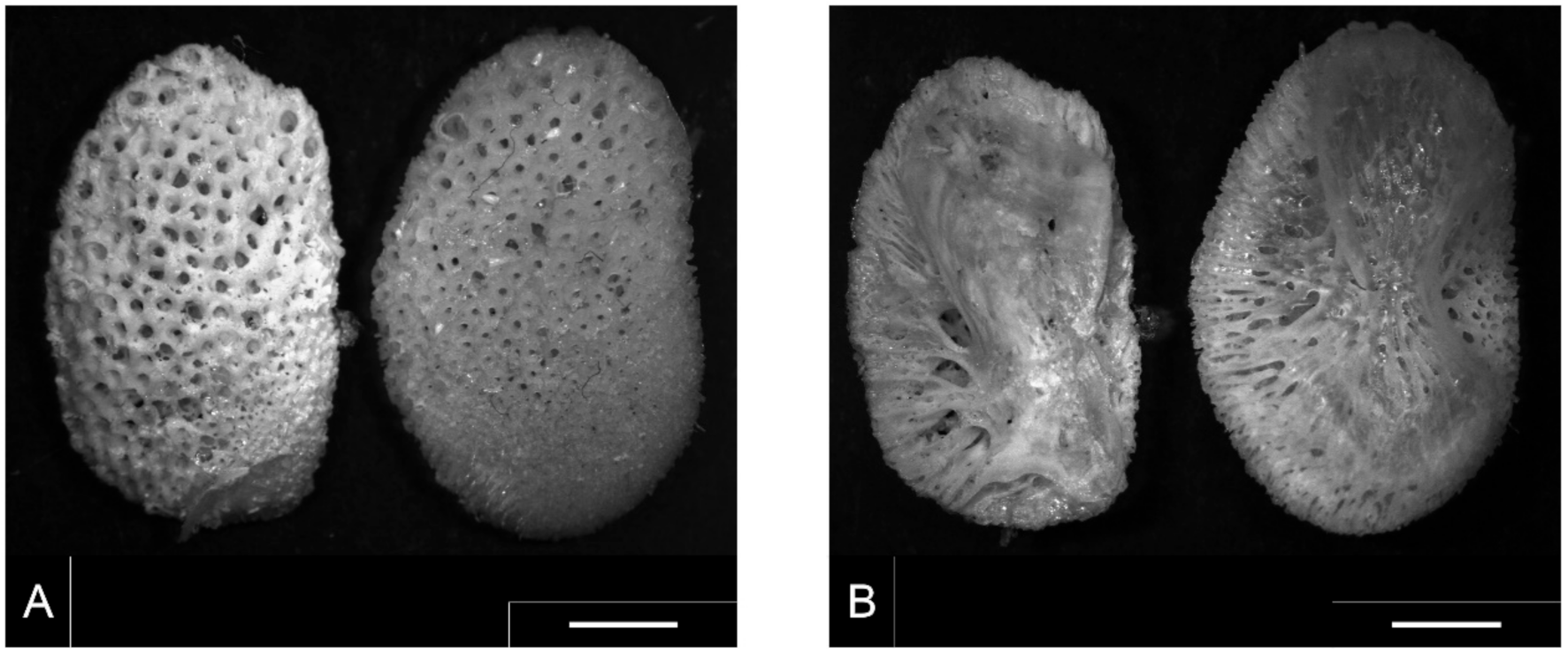
Following Smiroldo et al. [9], who reported a pharyngeal element and the caudal vertebrae as diagnostic items for S. glanis identification, we microscopically analyzed the skeleton of 27 differently sized specimens from our laboratory collection. The pharyngeal elements from specimens prepared in the laboratory showed many little cone-shaped teeth onto their outer surface; these teeth were completely lacking in samples found in stools likely because of the transit through the otter’s digestive system. This pharyngeal element was completely lacking in the skeletons of all the other considered fish species, except for the two catfish species. The comparison of these elements in S. glanis and I. punctatus is shown in Figure 1 (on the left and right, respectively, in each photograph).

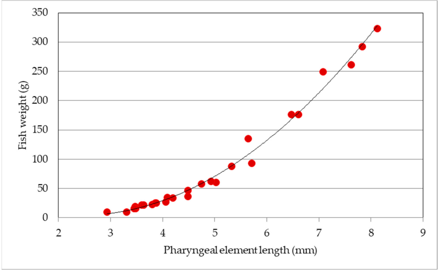
Dental plates of both species showed some similarities but also some differences. The general morphology was quite similar: the shape looked like a spongy bean with the outer surface provided with a great number of small alveoli (Figure 1A). The inner face was characterized by an asymmetric supporting main structure and by few minor branch-like formations reaching the lateral edge of the plate (Figure 1B). Despite the similar general structure, the dental plate from S. glanis differed, e.g., from that of I. punctatus, by several features: the shape was more oval in S. glanis, the dental alveoli were thicker and smaller in I. punctatus than in S. glanis, and the bone plate opposite the toothed surface was divided into two lobes in I. punctatus, while it was polymorphous in S. glanis. Species identification is quite simple, but it requires a direct comparison of unknown samples with those in the laboratory collection. To our knowledge, no previous relationships for the back-calculation of the original fish size were proposed for these elements in the literature, and, although they are less frequent and more difficult to recognize than vertebrae, they represent useful tools for species identification and size back-calculation, which can be subsequently used in the diet determination of piscivorous predators. Since in fish the pharyngeal element was present in pairs, and the differences between pairs in our laboratory collection were negligible (the mean coefficients of variation between pairs were 0.97% and 2.0% for the length and width, respectively), we measured the length and width of both from all the specimens of the laboratory collection and we considered their mean values (Table S2). The two dimensions were both related to the known fish weight (polynomial regressions: R² > 0.967; n = 27; p < 0.001), but the best fit was obtained with the length of the pharyngeal element (R² = 0.989) described by the equation: y = 9.906 x² − 47.617 x + 61.174 (Figure 2).

3.2. S. glanis Identification by Vertebra

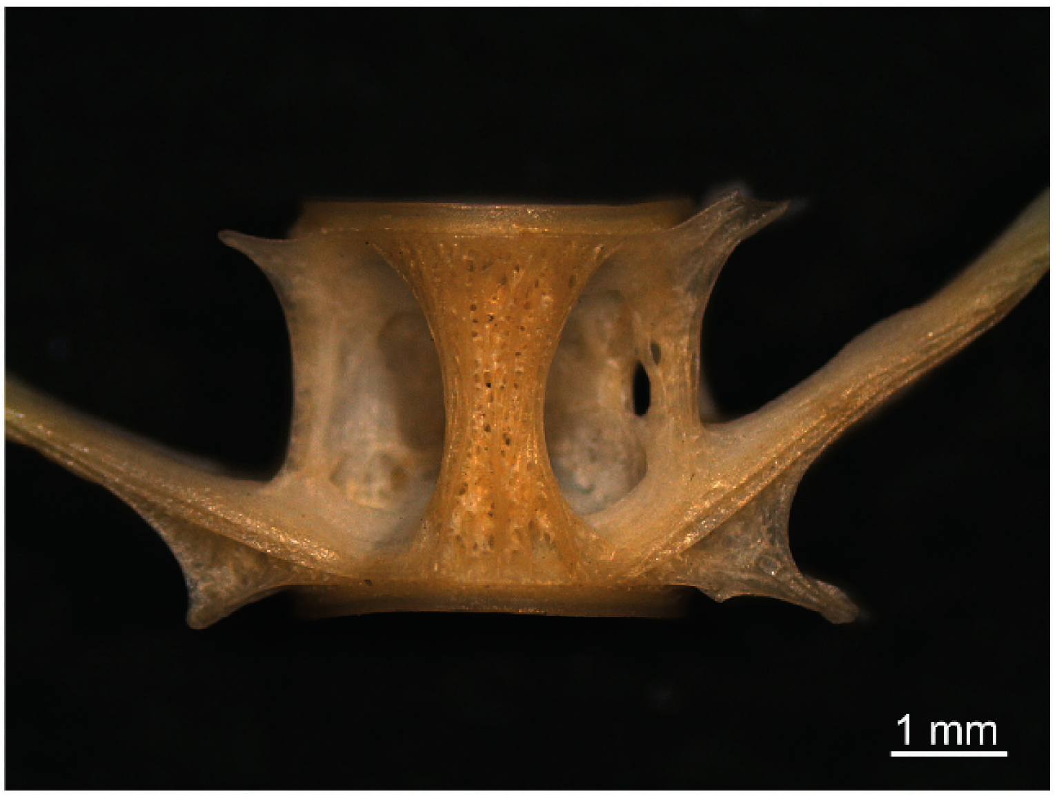
The second diagnostic element, also the most frequently recorded in stools, was represented by caudal vertebrae, in particular by the vertebral body, which, being well resistant to mechanical stress, was suitable not only for species identification but also for back-calculation of the original fish size. Vertebral processes are known to be useful tools for species identification [17], but they were not used here, as they represented weak structures that might be deeply damaged during the mastication and feeding processes, as observed in the otter stools. However, we found that the typical alveolar structure with a large hourglass rib of the vertebral body of S. glanis was a diagnostic element for species identification (Figure 3).

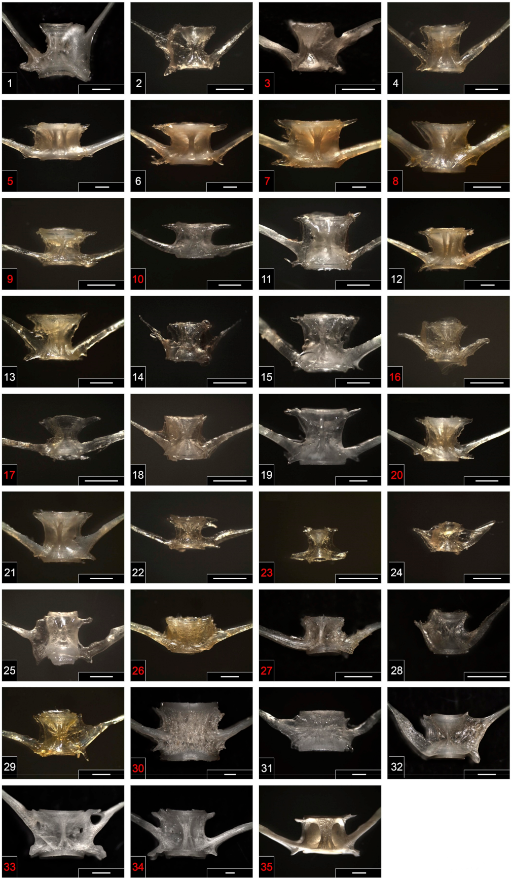
Figure 4 shows the morphology of the caudal vertebrae of the species living in the Ticino River and coming from our laboratory collection.

Table 1. List of autochthonous (black) and allochthonous (red) species living in the Ticino River, IUCN classification, and abundance score (Ab.): 1 = rare; 2 = present; 3 = frequent; 4 = abundant; 5 = dominant as in Moyle and Nichols [18]. Species names shaded in gray are shown in Figure 5.

Order	Family	Species	IUCN Red List	Ab.
Acipenseriformes	Acipenseridae	Acipenser naccarii†	VU	1
Anguilliformes	Anguillidae	Anguilla anguilla	CR	2
Cypriniformes	Cobitidae	Cobitis taenia	LC	3
		Misgurnus anguillicaudatus	-	3
		Sabanejewia larvata	LC	1
	Cyprinidae	Abramis brama	-	1
		Alburnus alburnus	DD	4
		Aspius aspius	-	1
		Barbus caninus	EN	2
		Barbus plebejus	LC	4
		Blicca bjoerkna	-	3
		Carassius carassius	-	3
		Chondrostoma soetta†	EN	1
		Ctenopharyngodon idella	-	1
		Cyprinus carpio	-	2
		Gobio gobio	LC	4
		Leuciscus cephalus	LC	5
		Leuciscus souffia	LC	4
		Phoxinus phoxinus	LC	3
		Protochondrostoma genei	LC	1
		Pseudorasbora parva	-	4
		Rhodeus sericeus	-	5
		Rutilus erythrophthalmus	LC	3
		Rutilus pigus	DD	2
		Rutilus rutilus	-	5
		Scardinus erythrophtalmus	LC	2
		Tinca tinca	LC	2
Cyprinodontiformes	Poecilidae	Gambusia holbrooki	-	2
Esociformes	Esociformi	Esox lucius†	LC	2
Gadiformes	Lotidae	Lota lota	LC	1
Gasterosteiformes	Gasterosteidae	Gasterosteus aculeatus	LC	1
Perciformes	Blennidae	Salaria fluviatilis	LC	2
	Centrarchidae	Lepomis gibbosus	-	3
		Micropterus salmoides	-	3
	Gobidae	Knipowitschia punctatissima	NT	2
		Padogobius martensii	LC	3
	Percidae	Perca fluviatilis	LC	2
		Stizostedion lucioperca	-	2
Petromyzontiformes	Petromyzontidae	Lethenteron zanandreai	LC	1
Salmoniformes	Salmonidae	Oncorhynchus mykiss	-	2
		Salmo (trutta) marmoratus†	LC	1
		Thymallus thymallus	LC	1
Scorpaeniformes	Cottidae	Cottus gobio	LC	1
Siluriformes	Ictaluridae	Ictalurus melas	-	1
		Ictalurus punctatus	-	1
	Siluridae	Silurus glanis‡	-	4

^† = Species with active Conservation Program. ^‡ = Species with active Containing Campaign.

reports an updated list of the Ticino River fish, based on recent samplings (2019) carried out for the LIFE project “Ticino BioSource” (LIFE15 NAT/IT/000989).

Based on the morphology of the vertebral body, some species were very different, such as Anguilla anguilla, which had an evident enlargement of the spine base (Figure 4(1)), or Aspius aspius, which had two hourglass ribs (Figure 4(5)); other species, such as trout, which had a spongy honeycomb aspect of the wall of the vertebral body but no ribs (Figure 4(30–31)), or Ictalurus punctatus and I. melas, which are phylogenetically close to S. glanis, showed similar hourglass reinforcements but without the same alveolar structure found in S. glanis (Figure 4(33–35)). Vertebral processes were also significantly different and should be considered as well, but they were not used here, as they represented weak structures that might be deeply damaged during the mastication and feeding processes as reported before. The vertebral body, being more resistant to mechanical stress, was considered suitable both for species identification and for the back-calculation of the fish size.

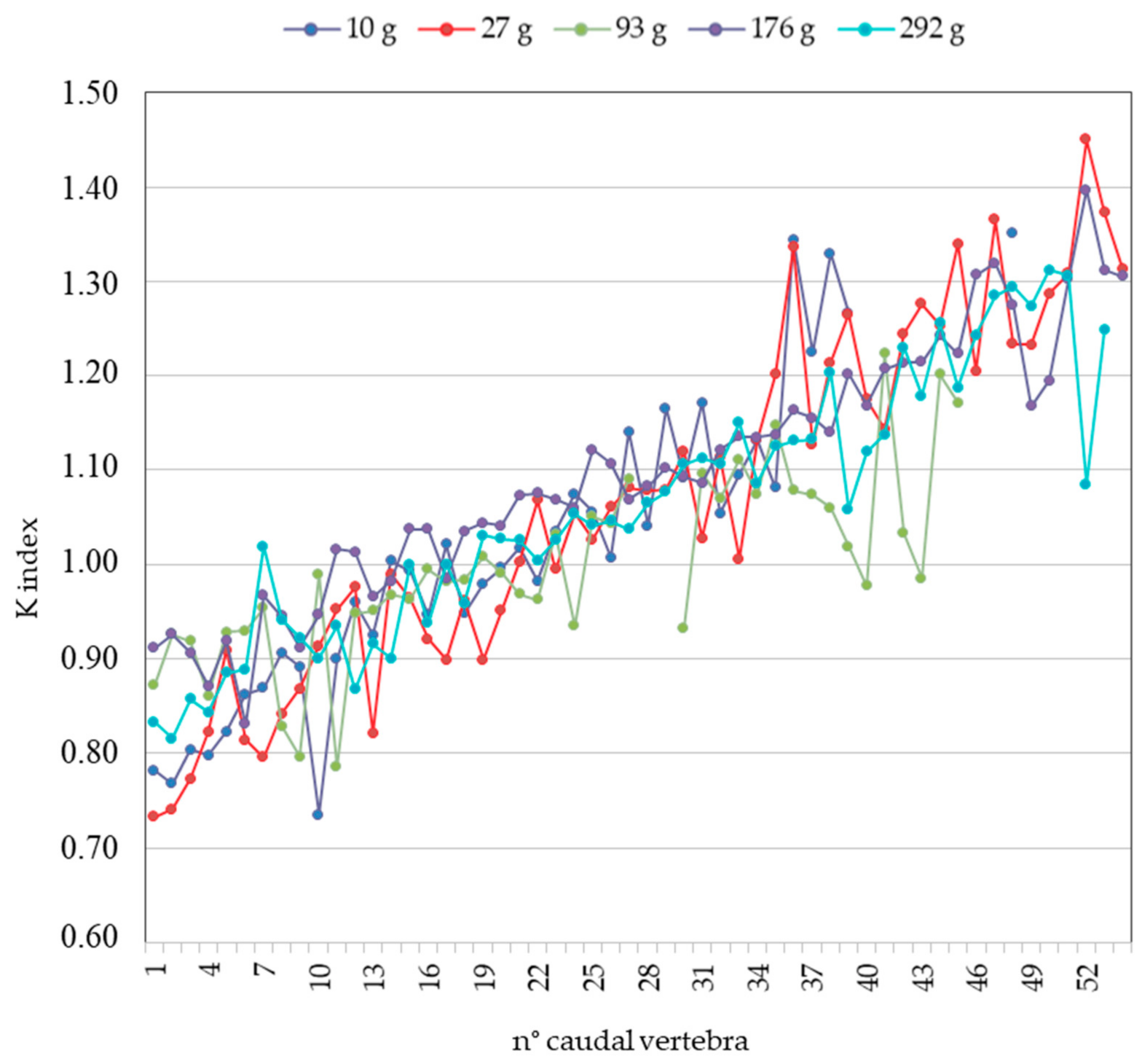
Unfortunately, differently from the pharyngeal elements, vertebrae presented some problems in the back-calculation procedures: in fact, fish of the same size could have vertebrae of very different sizes, depending on the relative position along the column. As discussed later, vertebral morphology varies along the vertebral column, and bone remains in otter stools are usually limited in number, sometimes damaged, such that the sole morphological approach may not be applicable for identifying the position along the column. For this reason, a quantitative tool able to identify the position of each vertebra along the column would be very useful in this kind of analysis. We thus selected from our collection five S. glanis samples with a total weight ranging between 10 and 292 g (Table S1), and we measured the length and the mean diameter of all caudal vertebrae from each specimen to find and then propose an index that allows one to identify the vertebral position along the column. We found that the ratio between the length and the mean diameter of the vertebral body was a good index for our purposes because it increased along the vertebral column in the cephalo-caudal direction between 0.7 and 1.4 for all the considered fish, independently from their size. We defined this as the K-index (Figure 5).

The increase in the K-index along the column depended on the fact that the mean diameter (denominator) decreased more rapidly than the vertebral length (numerator). Considering the numerical range of the K-index (0.7–1.4), for practical reasons, we divided it into five biometric groups: 0.7 to 0.9; >0.9 to 1.0; >1.0 to 1.1; >1.1 to 1.2; >1.2 to 1.4. The first and the last group presented an interval higher than the others because, at the beginning and at the end of the vertebral column, the K-index values varied greatly for a lower number of vertebrae, more than in the central portion of the column. The K-index values of each vertebra of the five fishes were significantly related to the five K groups (GLM: F_4;219 = 521; p < 0.001)—not to the fish to which they belong (GLM: F_4;219 = 0.70; p = 0.59)—and therefore to the fish size. Even the interaction between groups and fish was not significant (GLM: F_16;219 = 1.29; p = 0.21), meaning that there were no differences in the K-index values of the vertebrae among the five groups depending on fish size.

The number of vertebrae falling in each group ranged between 7 and 13, the mean value of the K-index of the vertebrae falling in the same group was very similar to the central value of the interval, and the 95% confidence interval of each group was very near to the mean value (

Table 2. Central and mean values of the K-index in the five K groups.

K Group	Central Value	Mean	95% CI
0.7–0.9	0.8	0.84	0.821–0.852
>0.9–1.0	0.95	0.95	0.942–0.962
>1.0–1.1	1.05	1.05	1.041–1.060
>1.1–1.2	1.15	1.14	1.127–1.156
>1.2–1.4	1.3	1.27	1.253–1.283

).

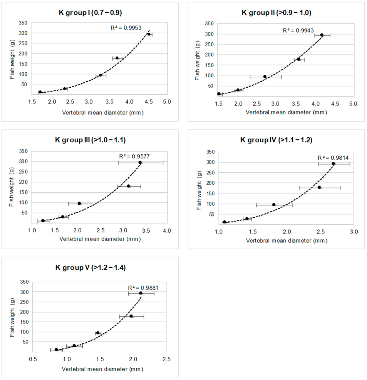
Once the method to assign each vertebra to a specific group was identified, we were able to define five quantitative relationships for calculating the fish weight from the vertebral size. The mean diameter was chosen as the “best vertebral size parameter” because it showed a greater variability range along the vertebral column than the vertebral length. In fact, the lower interval of vertebral length would have generated a lower precision in fish mass determination. Therefore, the mean diameter of the vertebrae belonging to each group was related to the known fish weight, obtaining five regression equations shown in Figure 6 and reported in

Table 3. Regression equations of the five K groups.

K Group	Equation	R2	p
I	y = 1.254 x3.6517	0.99	<0.001
II	y = 30.359 x2 − 69.158 x + 45.018	0.99	<0.001
III	y = 5.434 x3.2412	0.96	<0.001
IV	y = 7.842 x3.6157	0.98	<0.001
V	y = 18.056 x3.6038	0.99	<0.001

.

In this way, a vertebra found in otter feces can be assigned by its K-index to a ”K”-group, and the weight of a predated individual, as it was before ingestion, can be deduced through the relationship between the mean diameter and the fish mass of that group.

3.3. Model Validation

To verify this approach and to assess the variability derived by the back-calculation procedure, a model validation was performed with an independent set of data. For this purpose, three new S. glanis specimens were selected having low, medium, and high weight to back-calculate their known weights starting from their vertebrae.

Table 4. Fresh and back-calculated weights (±SD) of three S. glanis samples from our laboratory collection. Back-calculated weights were obtained from each vertebra of each K group.

	S. glanis Weight (g)
Fresh weight	20	60	323
Calculated Group I	18.4 ± 1.7	54.9 ± 1.2	366 ± 26
Calculated Group II	22.2 ± 3.5	69.8 ± 8.6	309 ± 35
Calculated Group III	24.0 ± 4.3	70.8 ± 13.8	355 ± 84
Calculated Group IV	19.4 ± 5.0	71.2 ± 11.5	371 ± 126
Calculated Group V	18.6 ± 6.3	67.1 ± 26.8	338 ± 98
Mean weight	20.4 ± 4.9	67.5 ± 17.7	347 ± 88
Coefficient of variation (%)	24	26	25

reported the known fish mass of the three selected fish and the mean back-calculated fish mass for each k-group and for each fish, with the mean coefficient of variation of the calculated masses derived by all vertebrae divided in the five k-groups by means of their K-indexes.

Calculated fish masses were very similar within the five k-groups (mean coefficient of variation ranging between 2.2% and 34%) and among groups (mean coefficient of variation ranging between 7.2% and 12%). The overall mean coefficient of variation of the calculated fish masses coming from all the vertebrae of all fish was 25%. In addition, mean calculated fish masses were very similar to the known fish mass values (mean percentage difference between calculated and known fish mass was 7.6%).

3.4. Back-Calculation of the S. glanis Size in Otter’s Stools

In the case of predictions of unknown fish masses from vertebral remains found in spraints, we can suppose that, when several vertebrae found in the same stool gave the same fish weight, we assumed that they belonged to the same specimen, whereas, when different vertebrae provided different fish weights, we assigned them to different individuals. For defining the weight similarities between two back-calculated fish masses, the mean variability derived from the proposed back-calculation procedure was considered. Therefore, two back-calculated weights belonging to different fish were considered if they differed by more than 30% (percentage difference between the two back-calculated weights).

In this work, 13 bony components from 8 different stools were analyzed (12 caudal vertebrae and 1 pharyngeal element), and the obtained back-calculated fish masses are reported in

Table 5. Back-estimation of S. glanis weights from bone remain analysis.

Stool ID	Sampling Date (DDMMYYYY)	Bone Remain	Mean Diameter (mm)	Height (mm)	K Index	K Group	Estimated Weight (g)
Ticino 25	22/10/2016	c v	4.31	3.43	0.8	I	260
Ticino 26	22/10/2016	c v	0.99	1.03	1.04	III	5
Ticino 26	22/10/2016	c v	1.98	1.69	0.86	I	15
Ticino 27	10/09/2016	c v	3.25	3.6	1.11	IV	556
Ticino 28	10/09/2016	c v	3.22	3.25	1.01	III	240
Ticino 57	28/01/2017	c v	2.58	2.87	1.11	IV	241
Ticino 58	28/01/2017	c v	0.86	1.19	1.38	V	10
Ticino 58	28/01/2017	c v	0.73	1.13	1.55	V	9
Ticino 61	28/01/2017	c v	2.26	1.7	0.75	I	25
Ticino 61	28/01/2017	c v	1.4	1.44	1.03	III	16
Ticino 61	28/01/2017	c v	1.54	1.58	1.03	III	22
Ticino 95	18/03/2017	c v	1.8	2.2	1.22	V	150
Ticino 58	28/01/2017	p e		2.75 a			5

c v = caudal vertebra. p e = pharyngeal element. ^a = length of the pharyngeal element (mm).

.

According to our methodology, diagnostic elements in the same stool were attributed to the same individual if the resulting fish weights were similar (within a 30% difference). An example of two elements very likely belonging to the same fish are those whose estimated weights were 10 and 9 g in the sample Ticino 58 reported in Table 5. On the contrary, when estimated fish weight was very similar, but the diagnostic elements came from different stools, they were attributed to different individuals (e.g., the estimated fish weights of 240 and 241 g in Ticino 28 and Ticino 57, respectively, Table 5). A third possibility was the finding of diagnostic elements in the same stool, giving very different estimated weights (e.g., estimated weights of 5 and 15 g in Ticino 26, Table 5). In this case, two different specimens were considered. In total, 10 individuals in 8 stools were identified, and the mean weight of the preyed S. glanis was 150 ± 179 g, within a range of 5–556 g. Fish weight is an important parameter in evaluating an otter’s diet, because it allows one to establish the relative contribution of the species in the overall diet, but for S. glanis population dynamics, the length and the age of the preyed fish should be considered as well. In the Ticino River, the S. glanis population was studied during containment campaigns, and the relationships between weight and length and between length and age were determined [19]. These relationships were as follows: fish weight (g) in natural logarithm = −11.279 + 2.897 * total length (mm) in natural logarithm (R² = 0.96), and total length (mm) = 1900.041 * (1 − exp (−0.098 * (fish age (years) + 0.74))) (R² = 0.96), respectively. By these equations, the mean length of the preyed S. glanis was 224 ± 129 mm, with a range of 85–435 mm and the mean age of the preyed S. glanis was 0.64 ± 0.72 year, with a range between 0+ and 2+ years. Length distribution of preyed S. glanis specimens showed that the most preyed class was between 250 and 350 mm and about 1 year old.

4. Discussion

Due to the increasing diffusion of alien species, a deep knowledge of the interactions between native and non-native species is a crucial goal to be achieved for drawing future conservation strategies. In the Ticino River, S. glanis has been detected since 1994, initially as occasional species, but it was defined as abundant as early as 1998 [19]. The Ticino River’s S. glanis population came from the Po River and since grew very quickly. In 2003, the Park authority promoted a containment campaign, as a conservation action for autochthonous species, in particular for the conservation of the critically endangered Acipenser naccarii, an endemism of the Po River basin [19]. Campaigns for S. glanis containment along the Ticino River are still ongoing, and in this context, the identification of S. glanis remains in otter stools in [9] represented an important finding. Unfortunately, no specific analyses were performed in that paper, and no indications of the number and the size of the preyed fish are yet available. For this reason, specific mathematical equations were developed to back-calculate the original fish size starting from S. glanis bone remains in feces. Two diagnostic elements (vertebrae and a pharyngeal bone) were selected. Otoliths, other elements often used in back-calculation procedures, were not considered here because they were not found. Indeed, otoliths are known to be subject to chemical degradation and possibly mechanical abrasion in the digestive tract of predators [20,21], making some species impossible to be recognized [22]. On the contrary, vertebrae and other bone remains were expected to be more resistant than otoliths and consequently more easily traceable in the feces of piscivore species [21]. For this reason, according to Feltham and Marquiss [23], Feltham [24], and Desse and Desse-Berset [25], they were proposed as suitable tools to estimate the minimum number of prey and to back-calculate their size.

Vertebrae have different characteristics useful in species determination, for example, the morphology of dorsal and ventral pre- and post-zygapophyses, the size and shape of neural and hemal spines, the sculpturing of the centrum, and the location and size of foramina [17,21]. Conroy et al. [26] suggested a key based on fish vertebrae considering 21 families, but they did not include S. glanis or other Siluriformes, nor did Hermsen and Maarseveen in the key that they suggested [27]. As already stated, we considered a typical alveolar structure with a large ‘hourglass’ rib of the vertebral body of S. glanis as a diagnostic element, since it was different from that of other fish species. Vertebral processes were not used here for species identification, as they represented weak structures that might be deeply damaged during the mastication and feeding processes as reported before.

In the literature, there are many equations for calculating fish size from vertebral length (e.g., equations from Thom [28] regarding trout). For S. glanis, a mathematical equation existed as well, but it was based only on the 13th thoracic vertebra [29]. As mentioned before, the main problem of using vertebrae in back-calculation is that, frequently, few recognizable vertebrae are found in feces, and since they can be very damaged, the determination of their relative position along the column may be uncertain. For this reason, the use of just one relationship for all vertebrae is not suitable. On the contrary, the proposed K-index was demonstrated (validation procedure) to be a quantitative tool for determining the position of each vertebra along the column and thus for back-calculating the fish mass of the prayed specimen with an acceptable accuracy (mean percentage difference between calculated and known fish mass was 7.6%). An additional advantage of the K-index was the fact that it could be calculated on the same vertebral body used for species identification and fish mass back-calculation. Moreover, the K-index methodology avoids the need to provide a number of equations equal to the number of the vertebrae and, therefore, the need to identify, vertebra by vertebra, the exact position in the vertebral column, which requires that all vertebral structures (spines, lateral apophyses, and zygapophyses) are not damaged (a rarely occurring condition). On the contrary, the K-index requires only two simple parameters: the mean diameter and the vertebral length.

The second element used in the species determination and back-calculation of fish mass was an oval pharyngeal element. These elements are involved in the function of retaining food items from the water flux crossing gills [15]. In light of the high number of teeth covering the whole surface of these elements, they can also furnish additional food fragmentation prior to entering the digestive system. These structures were lacking in all other species from the Ticino River, except for the two catfish species. As reported in the Results section (Figure 1), the dental plate from S. glanis differed from that of I. punctatus in several features: the shape appeared bean-shaped in I. punctatus and more oval in S. glanis, the dental alveoli were thicker and smaller in I. punctatus than in S. glanis, and the bone plate opposite the teeth bearing surface was divided into two lobes in I. punctatus, while it was irregularly shaped in S. glanis. Although less frequent and more difficult to recognize than vertebrae, these pharyngeal elements represented additional tools for species identification to be used in the diet determination of piscivorous predators. To our knowledge, no previous relationships were proposed for these elements in the literature.

5. Conclusions

The main conclusions of this work can be summarized as follows:

• The alveolar structure of the hourglass rib on the vertebral body of S. glanis is a diagnostic element for species identification, as are the shape and structure of the pharyngeal dental plate.
• The proposed K-index is able to identify the vertebral position along the column, independently from the fish size, and the set of predictive equations developed and validated in this work can establish the size of the preyed fish with a good level of accuracy.
• The back-calculation of the original size of preyed fish open new perspectives for more detailed studies on the diet of piscivorous predators as well as on control efficacy by the predation to prevent uncontrolled growth of allochthonous species.
• The proposed methodology applied to S. glanis remains in otter stools from the Ticino River revealed the predation of 10 specimens with weights ranging between 5 and 550 g, lengths between 85 and 435 mm, and ages between 0 and 2 years, with more frequent predation on specimens about 1 year old and 250–350 mm in length.

References

- Stone, R. The last of the leviathans. Science 2007, 316, 1684–1688. [Google Scholar] [CrossRef]
- Copp, G.H.; Bianco, P.G.; Bogutskaya, N.G.; Eros, T.; Falka, I.; Ferreira, M.T.; Fox, M.G.; Freyhof, J.; Gozlan, R.E.; Grabowska, J.; et al. To be, or not to be, a non-native freshwater fish? J. Appl. Ichthyol. 2005, 21, 242–262. [Google Scholar] [CrossRef]
- Hickley, P.; Chare, S. Fisheries for non-native species in England and Wales: Angling or the environment? Fish. Manag. Ecol. 2004, 11, 203–212. [Google Scholar] [CrossRef]
- Wysujack, K.; Mehner, T. Can feeding of European catfish prevent cyprinids from reaching a size refuge? Ecol. Freshw. Fish 2005, 14, 87–95. [Google Scholar] [CrossRef]
- Valadou, B. Le Silure Glane (Silurus glanis, L.) en France. Évolution de son Aire de Répartition et Prédiction de son Extension; Conseil Supérieur de la Pêche: Fontenay-sous-Bois, France, 2007. [Google Scholar]
- Copp, G.H.; Britton, R.J.; Cucherousset, J.; García-Berthou, E.; Kirk, R.; Peeler, E.; Stakenas, S. Voracious invader or benign feline? A review of the environmental biology of European catfish Silurus glanis in its native and introduced ranges. Fish Fish. 2009, 10, 252–282. [Google Scholar] [CrossRef]
- Prenda, J.; Clavero, M.; Blanco-Garrido, F.; Menor, A.; Hermoso, V. Threats to the conservation of biotic integrity in Iberian fluvial ecosystems. Limnetica 2006, 25, 377–388. [Google Scholar]
- Miranda, R.; Copp, G.H.; Williams, J.; Beyer, K.; Gozlan, R.E. Do Eurasian otters Lutra lutra (L.) in the Somerset Levels prey preferentially on non-native fish species? Fundam. Appl. Limnol. 2008, 266, 255–260. [Google Scholar] [CrossRef]
- Smiroldo, G.; Balestrieri, A.; Pini, E.; Tremolada, P. Anthropogenically altered trophic webs: Alien catfish and microplastics in the diet of Eurasian otters. Mammal Res. 2019, 64, 165–174. [Google Scholar] [CrossRef]
- Carss, D.N.; Kruuk, H.; Conroy, J.W.H. Predation on adult Atlantic salmon, Salmo salar L. by otters, Lutra lutra (L.) within the River Dee system, Aberdeenshire, Scotland. J. Fish Biol. 1990, 37, 935–944. [Google Scholar] [CrossRef]
- Kruuk, H.; Carss, D.N.; Conroy, J.W.H.; Durbin, L. Otter Lutra lutra numbers and fish productivity in rivers of North East Scotland. Symp. Zool. Soc. Lond. 1993, 65, 9–13. [Google Scholar]
- Weinberger, I.C.; Muff, S.; de Jongh, A.; Kranz, A.; Bontadina, F. Flexible habitat selection paves the way for a recovery of otter populations in the European Alps. Biol. Conserv. 2016, 199, 88–95. [Google Scholar] [CrossRef]
- Copp, G.H.; Roche, K. Range and diet of Eurasian otters Lutra lutra (L.) in the catchment of the River Lee (south-east England) since re-introduction. Aquat. Conserv. Mar. Freshw. Ecosyst. 2003, 13, 65–76. [Google Scholar] [CrossRef]
- Rutkayová, J.; Biskup, R.; Harant, R.; Šlechta, V.; Koščo, J. Ameiurus melas (black bullhead): Morphological characteristics of new introduced species and its comparison with Ameiurus nebulosus (brown bullhead). Rev. Fish Biol. Fish. 2013, 23, 51–68. [Google Scholar] [CrossRef]
- Rojo, A. Osteological Atlas of the Brown Bullhead (Ameiurus nebulosus) from Nova Scotia Waters: A Morphological and Biometric Study; Curatorial Report Number 100; Nova Scotia Museum: Halifax, NS, Canada, 2013. [Google Scholar]
- Schneider, C.A.; Rasband, W.S.; Eliceiri, K.W. NIH Image to ImageJ: 25 years of image analysis. Nat. Methods 2012, 9, 671–675. [Google Scholar] [CrossRef] [PubMed]
- Desse, G.; Du Buit, M.-H. Diagnostic des Pièces Rachidiennes des Téléostéens et des Chondrichthyens. III Téléostéens d’eau Douce; Expansion Scientifique Française: Paris, France, 1971. [Google Scholar]
- Moyle, P.; Nichols, R.D. Ecology of Some Native and Introduced Fishes of the Sierra Nevada Foothills in Central California. Copeia 1973, 3, 478–490. [Google Scholar] [CrossRef]
- Puzzi, C.M.; Trasforini, S.; Casoni, A.; Bardazzi, M.A.; Bellani, A. Il siluro (Silurus glanis). Ecologia della Specie nel Fiume Ticino e Risultati Dell’azione di Contrasto alla Sua Espansione Svolta dal Parco Negli Anni 2001–2006; Consorzio del Parco Lombardo della Valle del Ticino; Pontevecchio di Magenta: Milan, Italy, 2007. [Google Scholar]
- Pierce, G.J.; Boyle, P.R. A review of methods for diet analysis in piscivorous marine mammals. Oceanogr. Mar. Biol. Ann. Rev. 1991, 29, 409–486. [Google Scholar]
- Pierce, G.J.; Boyle, P.R.; Watt, J.; Grisley, M. Recent advances in diet analysis of marine mammals. Symp. Zool. Soc. Lond. 1993, 66, 241–261. [Google Scholar]
- Granadeiro, J.P.; Silva, M.A. The use of otoliths and vertebrae in the identification and size-estimation of fish in predator-prey studies. Cybium 2000, 24, 383–393. [Google Scholar]
- Feltham, M.J.; Marquiss, M. The use of first vertebrae in separating, and estimating the size of trout (Salmo trutta) and salmon (Salmo salar) in bone remains. J. Zool. 1989, 219, 113–122. [Google Scholar] [CrossRef]
- Feltham, M.J. The diet of red-breasted mergansers (Mergus serrator) during the smolt run in N.E. Scotland: The importance of salmon (Salmo salar) smolts and parr. J. Zool. 1990, 222, 285–292. [Google Scholar] [CrossRef]
- Desse, J.; Desse-Berset, N. Archaeozoology of groupers (Epinephelinae) identification, osteometry and keys to interpretation. Archaeofauna 1996, 5, 121–127. [Google Scholar]
- Conroy, J.W.H.; Watt, J.; Webb, J.B.; Jones, A. A Guide to the Identification of Prey Remains in Otter Spraints, 3rd ed.; The Mammal Society: London, UK, 2005. [Google Scholar]
- Hermsen, J.; Maarseveen, A.V. A Diet Study of the Eurasian Otter (Lutra lutra) Based on Spraint Analysis; Niewold Wildlife Infocentre: Leeuwarden, The Netherlands, 2011. [Google Scholar]
- Thom, T.J. The Ecology of Otters (Lutra lutra) on the Wansbeck and Blyth River Catchements in Northumberland; Durham E-Theses; Durham University: Durham, UK, 1990. [Google Scholar]
- Hensel, K. Find of a capital wels catfish Silurus glanis (Actinopterygii: Siluridae) in excavations of a Roman military fort in Southern Slovakia. Biologia 2004, 15, 191–203. [Google Scholar]
Figure 1.
Comparison between the pharyngeal element of S. glanis (on the left in each photograph) and I. punctatus (on the right in each photograph). (A) = dorsal view; (B) ventral view. Bar = 2 mm.
Figure 2.
Relationship between the length of the pharyngeal element and fish weight (y = 9.906 x2 − 47.617 x + 61.174; R2 = 0.989).
Figure 3.
Detail of the vertebral body from a caudal vertebra of S. glanis.
Figure 4.
Comparative photographs of the vertebral body from most of the fish species living in the Ticino River. White number = Autochthonous species; red number = Allochthonous species. Bar = 1 mm. 1 = Anguilla anguilla; 2 = Cobitis taenia; 3 = Misgurnus anguillicaudatus; 4 = Alburnus alburnus; 5 = Aspius aspius; 6 = Barbus plebejus; 7 = Blicca bioerkna; 8 = Carassius carassius; 9 = Ctenopharyngodon idella; 10 = Cyprinus carpio; 11 = Gobio gobio; 12 = Leuciscus cephalus; 13 = Leuciscus souffia; 14 = Phoxinus phoxinus; 15 = Protochondrostoma genei; 16 = Pseudorasbora parva; 17 = Rhodeus sericeus; 18 = Rutilus erythrophtalmus; 19 = Rutilus pigus; 20 = Rutilus rutilus; 21 = Scardinus erythrophtalmus; 22 = Tinca tinca; 23 = Gambusia holbrooki; 24 = Gasterosteus aculeatus; 25 = Salaria fluviatilis; 26 = Lepomis gibbosus; 27 = Micropterus salmoides; 28 = Knipowitschia punctatissima; 29 = Padogobius martensii; 30 = Perca fluviatilis; 31 = Salmo (trutta) marmoratus; 32 = Cottus gobio; 33 = Ictalurus melas; 34 = Ictalurus punctatus; 35 = Silurus glanis.
Figure 5.
Ratio between length and mean vertebral diameter (K-index) along the column in the cephalo-caudal direction in the considered samples.
Figure 6.
Regressions between the mean vertebral diameter and fish weight in the five selected K groups.